


Abstract
Conventional assessments of fault rupture propagation in overlying soil layers often rely on static or quasi-static analysis, neglecting the dynamic nature of fault displacement and inertial effects. This study develops a comprehensive simulation method for the entire process from rupture initiation to propagation under dynamic fault displacement. The method integrates a nonlinear elastic constitutive model based on the Hardin backbone curve with a non-uniform input technique for seismic waves on both sides of the fault using viscoelastic artificial boundaries. To demonstrate the distinct capabilities of this dynamic method, we conduct a comparative study on normal and reverse faulting driven by fault displacement time histories of identical magnitude but opposite sense. The simulations reveal that: (1) the fault displacement required for rupture initiation and propagation remains consistent between dynamic and quasi-static analyses; (2) crucially, the proposed method captures the transient dynamic response of fault rupture in the overlying soil. The study confirms that the proposed dynamic simulation framework is essential for resolving transient peak responses, oscillatory behavior, and deformation features associated with different faulting mechanisms, providing a more realistic tool for seismic risk assessment compared to conventional static approaches.
1. Introduction
Surface fault rupture, induced by fault dislocation, imposes severe site deformation on overlying soil layers, thereby threatening structures on the site or nearby. The accurate prediction of the deformation zone is therefore critical for the seismic design and risk assessment of infrastructure traversing active faults. In particular, the surface and near-surface deformation patterns are key determinants of structural performance.
Research worldwide on the influence of the overlying soil layers on near-surface deformation during fault dislocation has primarily followed three distinct approaches: (1) Statistical analysis, which establishes empirical relationships between earthquake magnitude and parameters such as surface displacement and fault rupture length based on post-earthquake field observation data using methods like statistical regression, to predict potential impacts of future earthquakes. Empirical relationships between earthquake magnitude and surface rupture parameters (e.g., length, width, and displacement) were established primarily from global datasets by Toeher, Bonilla, Coppersmith, and Xu [1,2,3,4], as well as the region-specific correlations established for China by Deng, Ye, and Tie et al. [5,6,7]. While this approach provides macro-level formulas, its accuracy is highly dependent on the quantity and quality of seismic damage records and often fails to adequately consider the specific characteristics of the overlying soil layers and the fault mechanism. (2) Experimental simulation, including techniques such as sandbox tests, geotechnical centrifuge tests, and shaking table tests, which offer intuitive and reliable insights into fundamental rupture modes and the influence of factors like soil density and layer thickness. Sanford, Emmons, Johansson, Lee, Liu, Shi, etc. [8,9,10,11,12,13,14] revealed the basic rupture patterns of soil under normal and strike-slip faults and the influences of factors such as soil water content, density, and layer thickness through sandbox tests; Roth, Bransby, Guo, Shen, etc. [15,16,17,18,19] used centrifuge tests to increase the gravity field to simulate the stress conditions of the prototype soil layer, better reflecting the true mechanical behavior of the soil. However, these methods are often constrained by equipment scale, model size, and cost, making it difficult to fully simulate complex geological conditions and deep source characteristics. (3) Numerical simulation, which involves establishing numerical analysis models to calculate and analyze various working conditions. Owing to its low cost, repeatability, and ability to handle complex conditions, numerical simulation has become the primary method. Researchers such as Scott, Bray, Loukidis, Zanjani, and Garcia [20,21,22,23,24,25,26], as well as Guo, Li, Zhao, and others [18,27,28,29,30,31], have systematically examined key parameters including fault type, dip angle, soil layer thickness and properties, and the presence of interlayers on the resulting rupture path and surface displacement. These studies have yielded significant insights into the failure mechanisms of overlying soil layers.
Based on existing research, significant insights have been achieved regarding the rupture of soil overlying faults. It is well established, for instance, that for a given amount of fault displacement, reverse faulting induces the most severe damage in the overlying soil layers, followed by normal faulting, with strike-slip faulting causing the least. Furthermore, the rock displacement of fault dislocation required to form a through-going rupture increases with soil layer thickness and is closely related to the fault dip angle and soil properties. However, a significant shortcoming in current research is that the vast majority of experimental and numerical simulation studies are based on static or quasi-static analysis, thereby neglecting the dynamic process of fault displacement and the associated inertial effects.
To address this limitation, this study develops a comprehensive dynamic simulation method for fault rupture in overlying soil layers. The method is validated through a comparative set of normal and reverse faulting cases constructed using identical geometric configurations, material properties, and fault displacement histories, with only the slip direction reversed, forming a pair of kinematically symmetric cases for direct comparison. By applying this unified dynamic method to both mechanisms and benchmarking the dynamic results against quasi-static analysis, the study directly isolates and quantifies the contribution of dynamic effects. This approach demonstrates the method’s capability to reveal how dynamic loading differentially amplifies the system response depending on the underlying fault mechanism, thereby confirming the necessity of a fully dynamic approach for accurate impact evaluation.
2. A Dynamic Rupture Simulation Method
This study presents a numerical framework to simulate the dynamic rupture of overlying soil layers induced by fault rock dislocation. The core of this framework entails (1) a constitutive model that captures the dynamic nonlinear stress–strain behavior of soil under large deformation, and (2) a technique for the non-uniform input of seismic waves on both sides of the fault.
2.1. Constitutive Model
2.1.1. A Nonlinear Model Based on the Hardin Backbone Curve
A nonlinear elastic constitutive model is employed to characterize the soil’s stress–strain behavior under dynamic loading. This model assumes fully recoverable deformation without hysteresis loops during unloading, offering the advantages of simplicity, few parameters, and straightforward calibration [32,33]. The hyperbolic relationship proposed by Hardin and Drnevich is a representative form of such a model, expressed in one-dimensional shear as:
where Gmax is the initial shear modulus, γ is the shear strain, and γ0 is the reference shear strain, obtained by fitting the Hardin-type hyperbolic model to the dynamic shear modulus reduction curve.
For implementation in explicit dynamic analysis, the total load is divided into increments, within which the soil is treated as linearly elastic with a tangent shear modulus, G, that is updated based on the current strain level according to the nonlinear backbone curve Equation (1). The relationship between the strain increment and the corresponding stress increment follows the generalized Hooke’s law:
where, λ and μ are the Lamé constants:
Here, ν is Poisson’s ratio and G is the tangent shear modulus for the current increment.
In the backbone curve described by Equation (1), the tangent modulus G asymptotically approaches zero as the shear strain increases. In explicit dynamic analysis, however, allowing the modulus to decrease to extremely small values may lead to severe mesh distortion and numerical instability. To maintain numerical stability, a cutoff is imposed: once the shear strain exceeds a threshold γm, the tangent modulus is fixed at 0.01Gmax, which represents the minimum allowable value in the numerical implementation. This cutoff is adopted as a numerical stabilization measure rather than a material parameter and does not imply additional plastic hardening or softening behavior. Therefore the tangent modulus is thus defined as:
2.1.2. Shear Strain Determination
The three-dimensional implementation of the constitutive model requires determining the tangent shear modulus G at each step. Following the approach of Dong et al. [34], the octahedral shear strain γoct is introduced as the equivalent shear strain, which serves as an equivalent scalar measure of three-dimensional shear deformation by representing the overall shear distortion intensity on octahedral planes (equally inclined to the three principal strain directions), enabling the representation of stresses and strains in Equation (4) in terms of equivalent shear measures. The octahedral shear strain is computed from the principal strains as:
where ε1, ε2, and ε3 denote the major, intermediate, and minor principal strains, respectively.
Extensive triaxial shear tests have shown that soils typically reach their ultimate bearing capacity when the shear strain develops to the range of 3–5%, after which they enter a fully plastic deformation stage. Since shear failure is the dominant cracking mode in soils, this strain range is commonly adopted in finite element analyses as a criterion to identify soil elements reaching a shear failure state, with the limiting shear strain defined as γmax = ε1 − ε3. In this study, the maximum shear strain is selected as the lower bound of this range, 3%.
To employ the equivalent shear strain γm as the failure criterion, a conversion relationship with γmax is required. For analysis convenience, γmax is normalized to 1, and the Lode angle parameter b is introduced, with its value ranging from 0 to 1:
The ratio R between the equivalent and maximum shear strains is then expressed as:
Under typical stress states, R attains approximately 0.943 for triaxial compression (b = 0), 0.816 for pure shear (b = 0.5), and 0.943 for triaxial extension (b = 1). Adopting a conservative approach, the minimum value R = 0.816 is selected. Accordingly, for a limiting shear strain γmax = 3%, the corresponding maximum equivalent shear strain in Equation (4) is taken as γm = 2.45%.
2.1.3. ABAQUS Subroutine
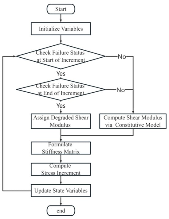
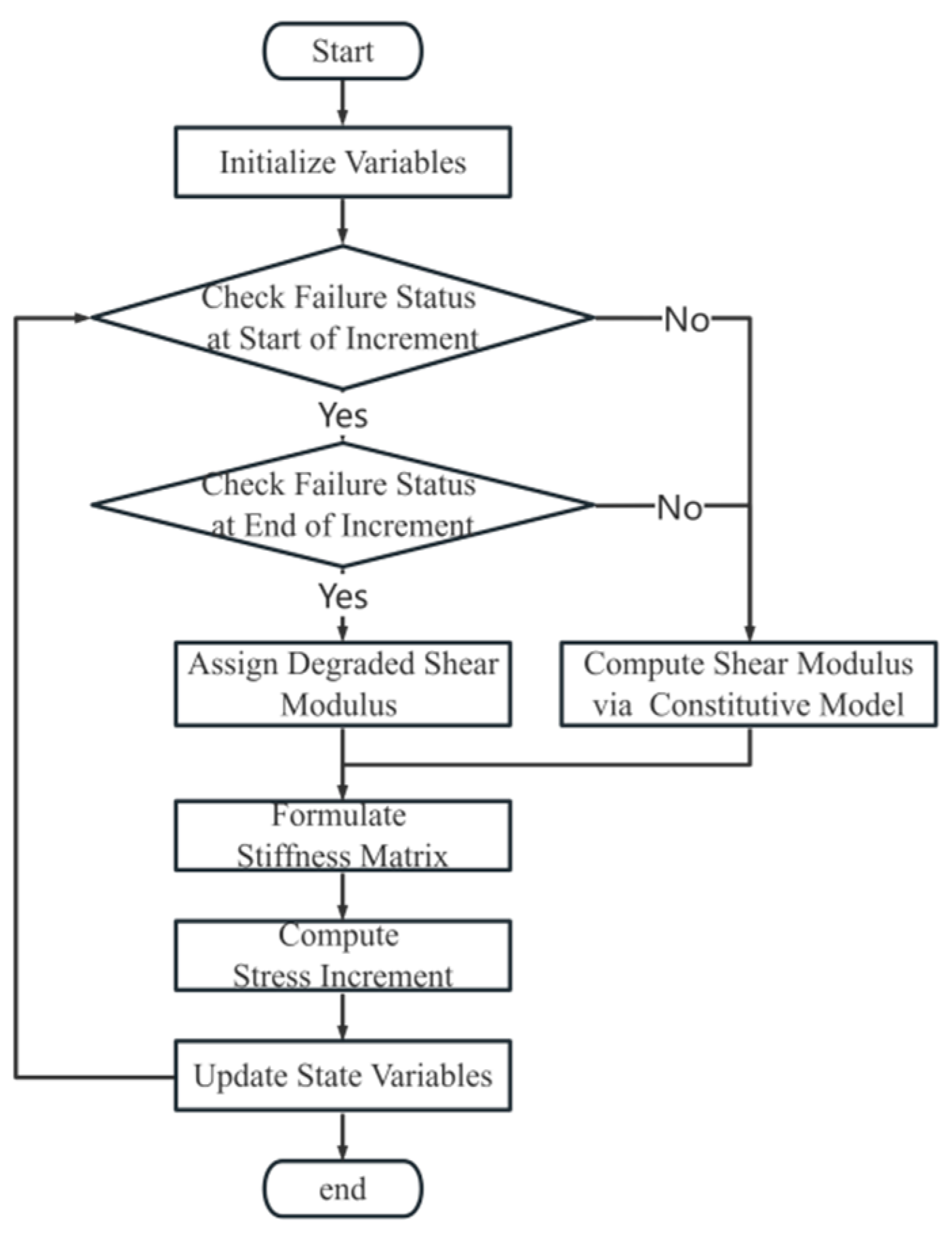
A VUMAT subroutine was developed in ABAQUS/Explicit (version 2021) to incorporate the nonlinear elastic constitutive model, the calculation flowchart of which is shown in Figure 1.
Figure 1.
Flowchart of the VUMAT subroutine.
2.2. Non-Uniform Seismic Input
Simulating the seismic dynamic response across a fault requires a rational implementation of non-uniform wave input on its two sides within the finite element model. To achieve this, viscoelastic artificial boundaries [35,36,37] are introduced, dividing the domain into a near-field finite region and a far-field infinite region. The far-field is treated as horizontally stratified, while the near-field can incorporate more complex, non-horizontal layering. This technique converts the infinite domain into an equivalent spring-dashpot system applied at the boundaries. By applying equivalent nodal forces derived from the free-field motion, the method effectively simulates the propagation of seismic waves from the far-field to the fault.
To enable independent wave input on each side of the fault, the fault itself is simplified as a smooth contact surface, and the influence of outgoing waves from the finite domain is neglected. The seismic input motions on both sides of the fault are applied to propagate approximately parallel to the fault plane. Under this constraint, the relative movement of the hanging wall and the footwall is mainly governed by shear deformation along the fault, while normal incidence and energy exchange across the fault interface are minimal. This assumption allows the wave fields in the two infinite domains to remain independent, permitting the separate specification of their respective input motions.
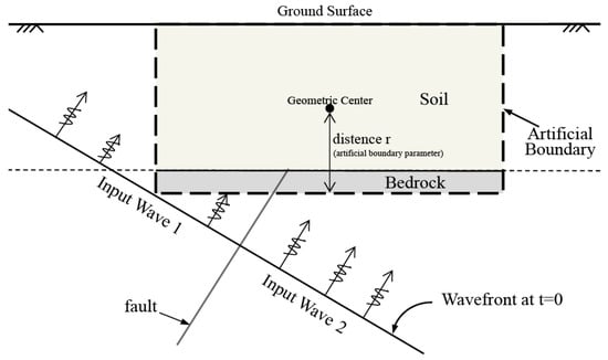
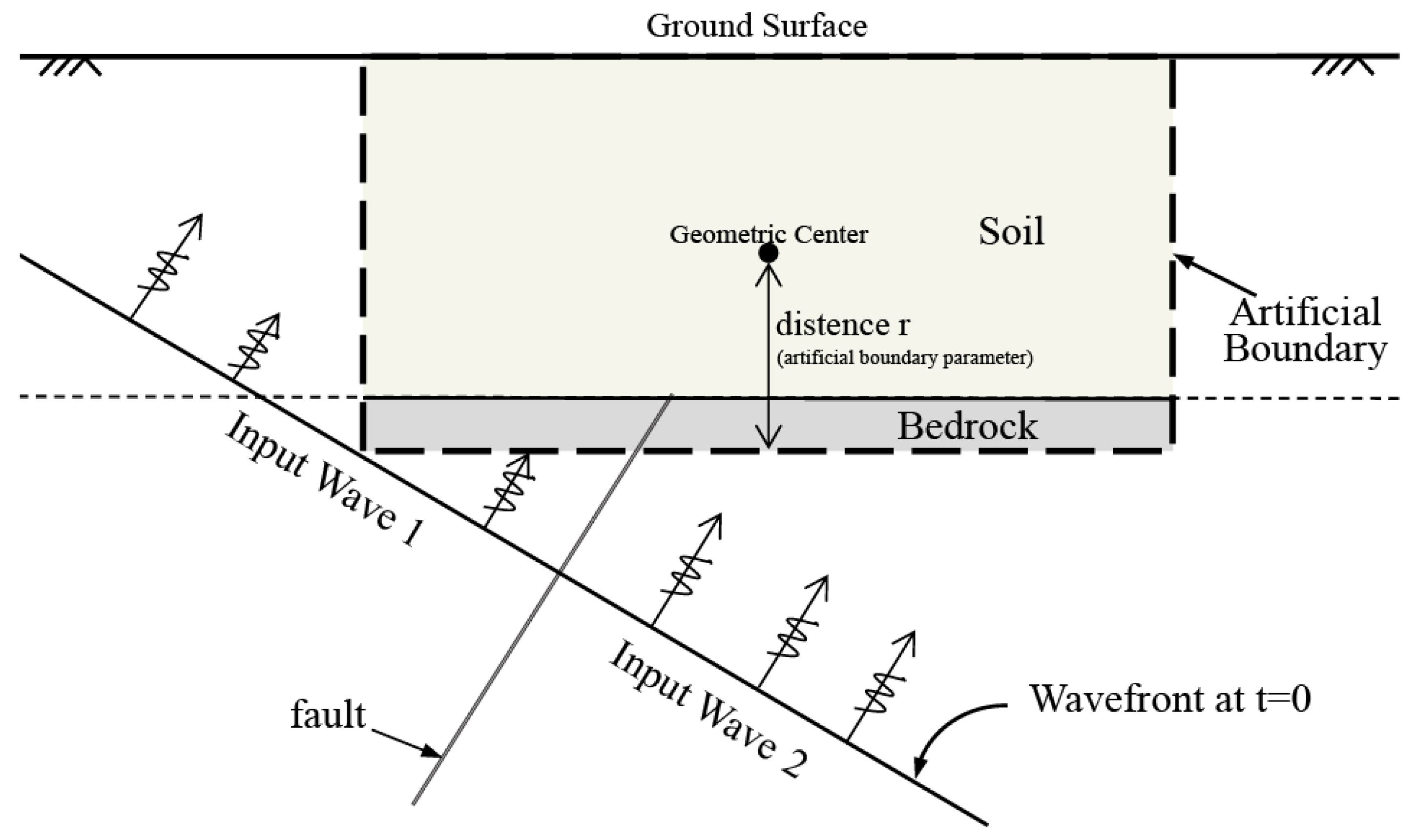
The computational domain, illustrated in Figure 2, is partitioned by artificial boundaries into a near-field finite region, capable of incorporating complex geology, and a far-field infinite region, idealized as horizontally layered. The bedrock fault further subdivides the infinite domain into two independent sections. To simulate the non-uniform wave input induced by fault dislocation, the free-field responses of the horizontally layered sites on each side are independently prescribed at their corresponding lateral artificial boundaries. Similarly, the segments of the bottom boundary on the hanging wall and footwall are driven by the free-field motion from their respective sides. This configuration effectively captures the differential movement across the fault.
Figure 2.
Schematic diagram of non-uniform seismic input on both sides of the fault.
Physically, the viscoelastic artificial boundary represents the influence of the unbounded exterior by applying one-way spring-dashpot elements at the boundary nodes, which absorb radiating energy and provide a restoring force.
The spring-dashpot parameters for the two-dimensional viscoelastic artificial boundary are defined as:
where λ and μ are the Lamé constants, ρ is the mass density, and cp and cs are the P-wave and S-wave velocities, respectively. The distance r is taken from the geometric center of the near-field structure to the boundary segment, and in this study r is taken as half of the model thickness. The artificial boundary parameters A and B were adopted from the viscoelastic boundary model proposed by Du et al. [36], in which A = 0.8 and B = 1.1 were recommended based on theoretical derivation and numerical verification.
The viscoelastic boundary is implemented as a stress boundary. The motion of the boundary nodes induces a stress response from the spring-dashpot elements, which is a function of the node displacement and velocity:
The equation of motion for a node on this boundary, incorporating the influence of both the finite and infinite domains, is:
Rearranging terms yields the final form of the node’s equation of motion:
where M, C, and K represent the mass, damping, and stiffness matrices, respectively; in the present free-field boundary analysis, C is set to zero (i.e., internal damping within the domain is neglected), and far-field energy dissipation is represented only by the boundary-damping coefficient CB; u, and denote the node displacement, velocity, and acceleration, respectively; and f is the applied node force. The parameter AB is the control area for the viscoelastic boundary node. For 2D problems, AB is obtained by summing half of the boundary edge length of all elements connected to that node. While for 3D problems, AB is calculated by summing one-quarter of the boundary face area of all elements connected to that node. The total force f acting on a boundary node is decomposed into two components:
- f1, the force required for the artificial boundary node to achieve a displacement uI against the resistance of the finite domain medium, determinable via the geometric and constitutive relations of the internal medium;
- f2, the force required to achieve the same displacement uI against the boundary spring-dashpot elements. This force is derived from the incident displacement field uI at the artificial boundary within the viscoelastic framework:
Therefore, the complete equation of motion under viscoelastic boundary conditions is:
This governing equation simultaneously accounts for the dynamic response of the internal medium, the mechanical behavior of the artificial boundary, and the input from the incident wave field. It thereby provides a comprehensive theoretical basis and a practical numerical methodology for simulating non-uniform seismic wave input on both sides of a fault.
2.3. Simulation Procedure
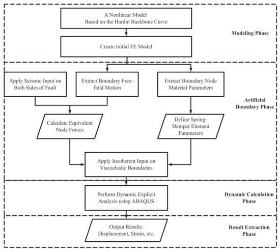
The simulation of rupture initiation and rupture propagation in overlying soil layers subjected to dynamic fault displacement between the two sides of a fault follows a procedure comprising four primary stages: (1) model establishment, (2) application of artificial boundaries, (3) execution of a dynamic explicit analysis, and (4) result extraction. The overall workflow is illustrated in Figure 3.
Figure 3.
Simulation workflow for fault rupture propagation through overlying soil layers.
During the model establishment phase, a bedrock layer of finite thickness is incorporated. This is necessitated by the wave-reflection characteristics at the soil-rock interface, which contrast with the non-reflective nature of the viscoelastic boundary applied at the model base. Introducing this bedrock layer thus enables a more physically realistic simulation of wavefield interactions. The bedrock material itself is simulated using a linear elastic constitutive model.
In scenarios involving a thin or non-existent fault fracture zone, the basal soil elements directly above the fault are susceptible to severe distortion under large fault displacement. To mitigate this numerical issue and prevent associated convergence difficulties, a layer of deletable cohesive elements is inserted at the soil-rock interface. This technique facilitates a gradual separation between the soil and bedrock, allowing the deformation imposed by the fault to be distributed across multiple soil elements, thereby alleviating excessive distortion in any single one.
3. Constitutive Model and Procedure Verification
The accuracy and reliability of the proposed dynamic rupture simulation method are demonstrated through two verification studies. First, a single-element test is conducted to validate the self-developed nonlinear elastic VUMAT subroutine’s capability in capturing soil nonlinearity and shear failure. Subsequently, a published quasi-static case is reproduced to verify the constitutive model’s performance under complex stress conditions and to indirectly assess the overall simulation procedure. It is noted that the theoretical foundation for the non-uniform input method, the viscoelastic artificial boundary, is well-established and has been extensively validated in prior studies [38,39,40].
3.1. Subroutine Verification
A single-element model was developed to verify the self-developed nonlinear elastic VUMAT subroutine within the ABAQUS/Explicit framework. The verification model consisted of a 1 m × 1 m plane strain quadrilateral element with its base fully fixed. A state of pure shear was simulated by applying a horizontal displacement of 0.1 m at the top nodes, followed by unloading of the same magnitude to return the element to its initial position. This loading path was designed to evaluate the constitutive model’s response throughout both loading and unloading phases.
The physical and mechanical parameters of the soil element are provided in Table 1 and Table 2. Parameters in Table 1 were derived from the published quasi-static case of Li et al. [29], whereas those in Table 2 were adopted from the laboratory test results of medium sand with comparable physical and mechanical properties. The shear strain γ0 in Table 1 was determined by fitting the dynamic shear modulus ratio curve given in Table 2.
Table 1.
Mechanical parameters of the overlying soil layer.
Table 2.
Dynamic parameters of the overlying soil layer.
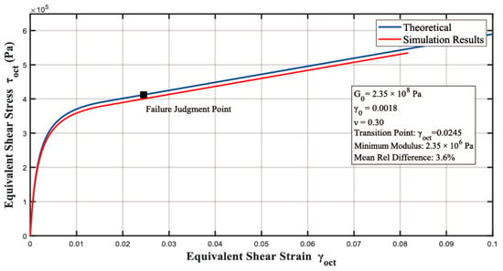
Figure 4 compares the simulated octahedral stress–strain relationship with the theoretical curve, showing close agreement between the two. The relative error in stress remains within 5% at identical strain levels. The theoretical curve was generated according to the constitutive formulation used in this study. It is based on the classical Hardin hyperbolic stress–strain relation Equation (1), but incorporates the modulus–degradation constraint expressed in Equation (4).
Figure 4.
Comparison of theoretical and simulated octahedral stress–strain relationships. The Theoretical curve is calculated using the modified Hardin-type model (Equations (1) and (4)), and the Simulation Results are obtained from the VUMAT simulations.
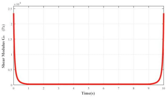
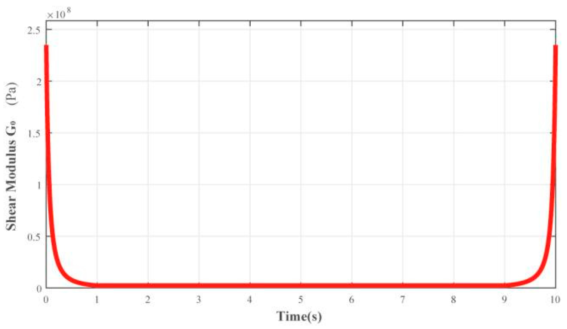
Figure 5 presents the time history of the shear modulus G, which exhibits gradual softening during loading and recovery upon unloading, consistent with theoretical behavior. After the specified shear failure, the shear modulus stabilizes at 1% of its initial value, accurately capturing the stiffness degradation and recovery mechanism.
Figure 5.
Time history of element shear modulus G.
These results confirm that the VUMAT subroutine correctly implements the intended nonlinear elastic constitutive model, ensuring its suitability for subsequent dynamic analyses of geotechnical systems.
3.2. Quasi-Static Verification Case
A published quasi-static case from Zhao [27] was replicated, to validate the accuracy of the nonlinear elastic constitutive model in simulating the failure of the overlying soil layer and to indirectly verify the overall simulation procedure. This benchmark model involves a 45° reverse fault rupturing through a 30 m thick sand layer.
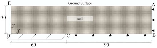
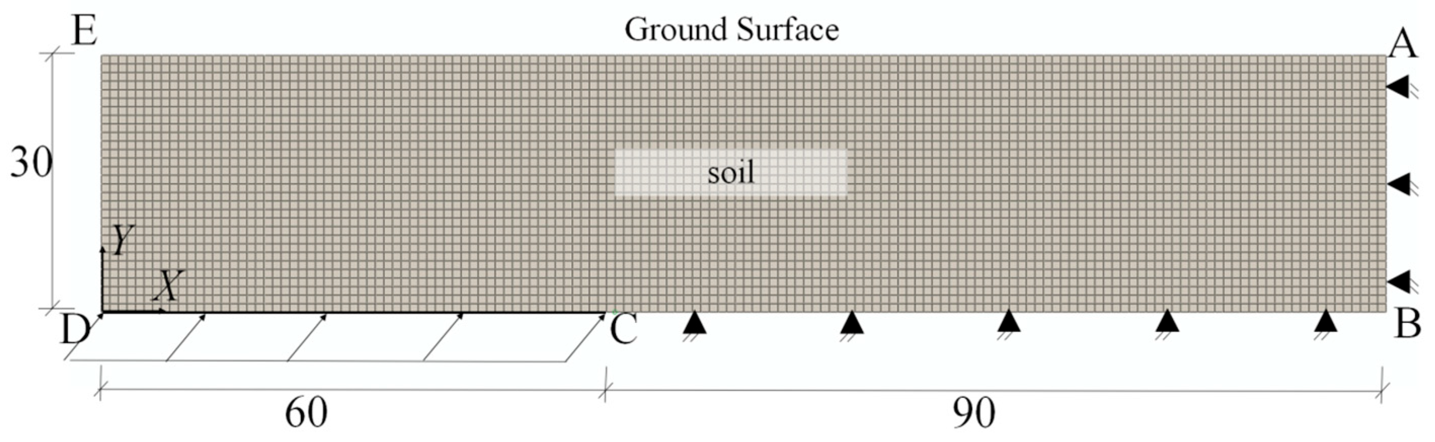
As shown in Figure 6, the model geometry is 150 m wide and 30 m high, with the fault trace located 60 m from the left boundary. The soil material parameters, identical to those in the reference, are listed in Table 3. The boundary conditions were also reproduced consistently: the AB and BC boundaries on the footwall side were fixed; the DE boundary on the hanging wall side was free; and the bottom boundary (CD) was subjected to prescribed displacements in the X and Y directions to simulate the 45° reverse fault displacement, achieving a final fault vertical offset of 1.20 m.
Figure 6.
Quasi-static analysis model.
Table 3.
Parameters of the overlying soil layer.
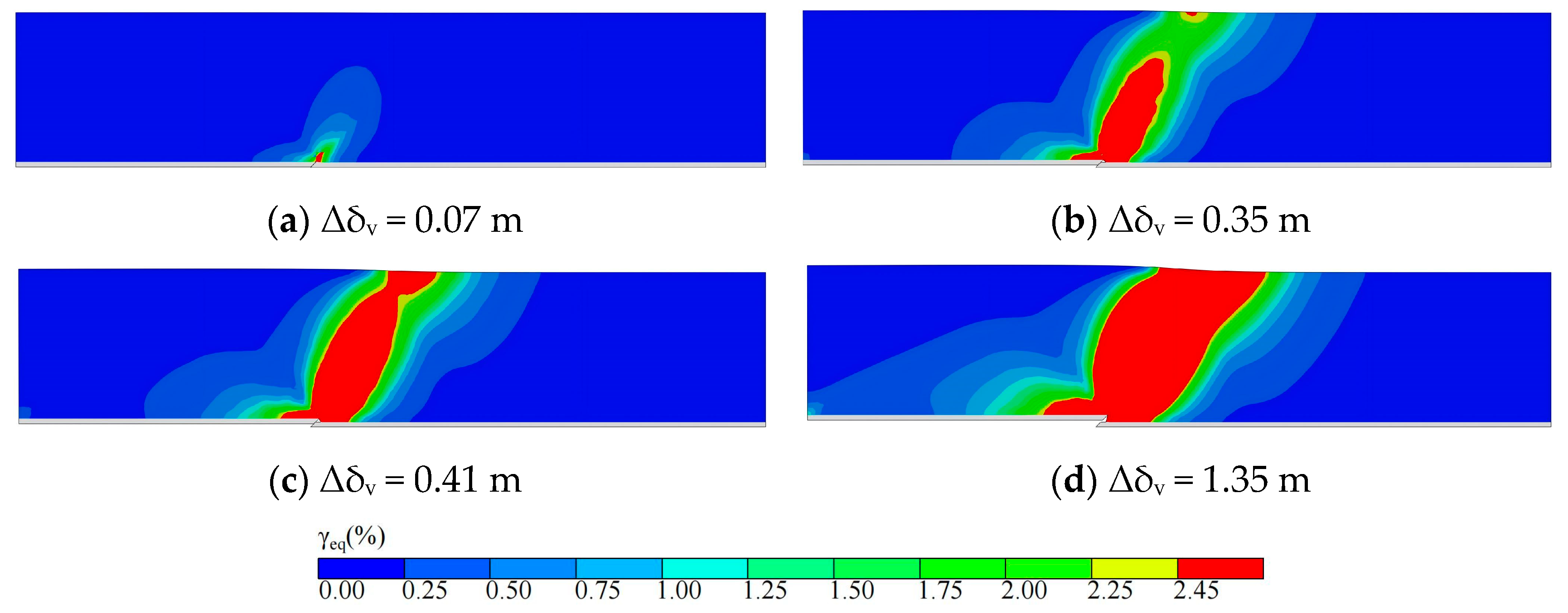
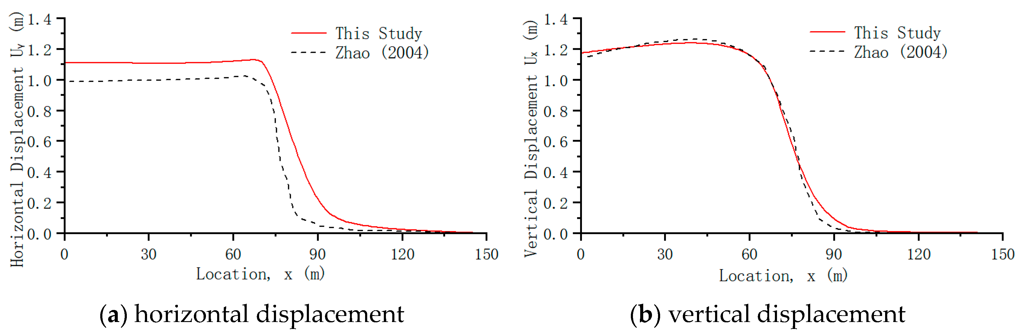
The simulated rupture propagation process is illustrated in Figure 7. Surface rupture initiates at a fault vertical displacement (Δδv) of 0.35 m (Figure 7b) and becomes fully continuous at Δδv = 0.41 m (Figure 7c). These results are in close agreement with the reference values of 0.329 m and 0.413 m, respectively, reported in the literature. A comparison of surface displacements at a final fault offset of 1.2 m is presented in Figure 8. The simulated vertical surface displacements match the reference data well; however, the horizontal displacements are generally higher than those in the benchmark study.
Figure 7.
Quasi-static simulation: equivalent shear strain contours for the reverse fault. Panels (a–d) correspond to successive rupture stages: (a) rupture initiation, (b) surface rupture emergence, (c) rupture fully connects, (d) final state of the simulation. Rupture criterion: Red regions denote the predicted rupture zone, defined by equivalent shear strain exceeding the prescribed critical threshold (Section 2.1.2), and the same rupture criterion and color scheme are adopted for all subsequent strain contour plots unless otherwise noted. Notation: Δδv denotes the relative vertical displacement across the fault and is used consistently in all subsequent figures.
Figure 8.
Comparison of surface displacements at a fault vertical displacement of 1.2 m. The results from Zhao (2004) are taken from [27].
These discrepancies primarily arise from the different constitutive models employed. The elasto-plastic model adopted in the reference study exhibits a stronger material softening capability, allowing a considerable portion of the shear strain to be accommodated at depth and thereby limiting the lateral deformation transmitted to the ground surface. In contrast, in the nonlinear elastic model used in this study, a lower bound is imposed on the tangent modulus so that softening is restricted once a certain degradation level is reached, resulting in a stronger overall deformation capacity and consequently larger horizontal displacement at the ground surface. Vertical displacement, being predominantly governed by the fault dip angle and displacement magnitude, remains essentially consistent between the two models.
In addition, a brief mesh sensitivity check was conducted for the quasi-static verification model to assess the robustness of rupture localization and strain concentration. Simulations with different mesh sizes (2 m, 1 m, 0.5 m, and 0.2 m) indicate that the overall rupture pattern, surface deformation trend, and the width of the high-strain zone are already well captured with a mesh size of 1 m. Further mesh refinement mainly results in smoother strain contours near local boundaries, without producing noticeable changes in displacement magnitude or rupture geometry. These observations suggest that the numerical results are not significantly affected by mesh discretization, and the adopted mesh density provides a reasonable balance between accuracy and computational efficiency.
In summary, the present simulation successfully reproduces the key characteristics of the benchmark case, including the rupture propagation and the pattern of surface deformation. Although minor differences exist in the precise fault displacement required for rupture and in the magnitude of horizontal surface displacement, these fall within acceptable tolerances. This comparison validates the capability of the proposed nonlinear elastic constitutive model to effectively simulate rupture propagation and deformation response in overlying soil layers subjected to fault displacement, justifying its use in subsequent dynamic finite element analyses.
4. Dynamic Fault Rupture Analysis
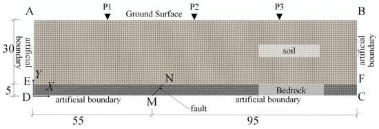
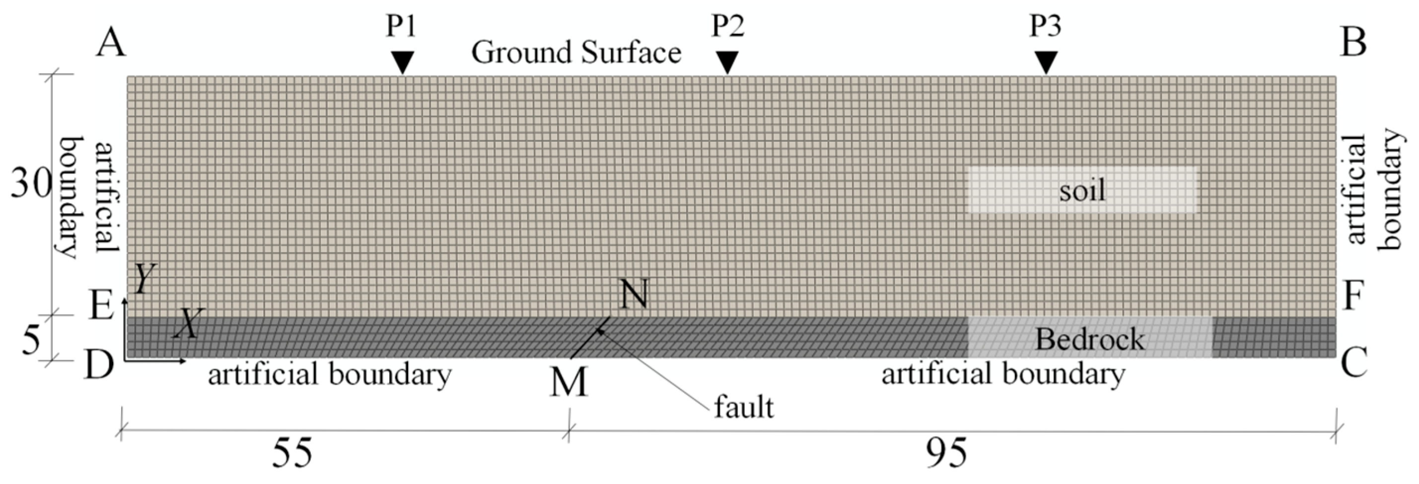
This section employs the same model configuration for dynamic simulations of both reverse and normal fault displacements, differing only in the direction of the imposed fault slip. The model, depicted in Figure 9, spans 150 m in width and 35 m in depth, comprising a 30 m thick soil layer overlying a 5 m thick bedrock layer. Model boundaries are labeled as follows: AB represents the free ground surface; EF denotes the soil-rock interface; CD is the bottom artificial boundary; AD and BC are the left and right artificial boundaries, respectively. The bedrock fault, MN, dips at 45°, with its upper tip located 60 m from the left model boundary, measured from point E to point N.
Figure 9.
Numerical model for the dynamic fault rupture analysis.
Viscoelastic artificial boundaries are applied to the left, right, and bottom edges of the model. The free-field response computed for the left-side domain is input at the left boundary (AD) and the left segment of the bottom boundary (DM). Similarly, the right-side free-field response is applied to the right boundary (BC) and the right segment of the bottom boundary (CM). Relative dynamic displacement across the fault is generated by applying equivalent node forces derived from distinct dynamic displacement time histories on each side of the fault.
For the material constitutive models, the overlying soil layer was simulated using the nonlinear elastic model, while the bedrock was modeled as linear elastic to account for wave reflection at the soil-rock interface. The corresponding material parameters are listed in Table 4.
Table 4.
Model Material Parameters.
Note that the dynamic simulations in this section are conducted using an idealized numerical model to enable controlled comparisons between reverse and normal faulting under dynamic loading (with the two cases differing only in slip direction). Therefore, the predicted deformation and strain patterns are interpreted primarily to elucidate rupture mechanisms, rather than to reproduce the detailed geometry of any specific field surface rupture.
4.1. Reverse Fault Dynamic Simulation
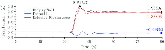
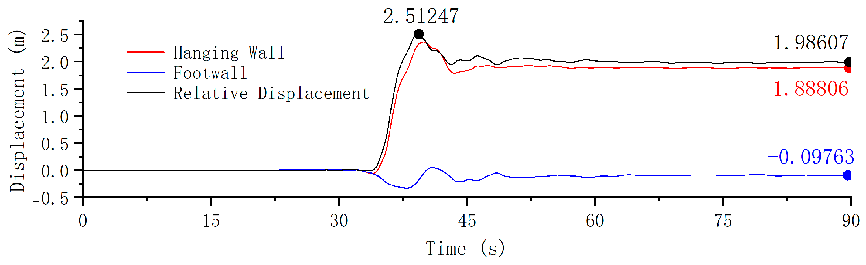
This example simulates the rupture propagation process through a 30 m thick overlying soil layer subjected to reverse fault dislocation. The input ground motions were derived from the records of the TCU-068 and TCU-103 stations during the Chi-Chi earthquake (Figure 10). These records are considered highly representative of reverse fault dislocation, as they clearly capture the permanent ground displacement associated with near-fault thrust motion. Their well-documented source characteristics and widespread use in fault rupture studies make them suitable benchmark inputs for investigating the dynamic soil response. The original records were scaled down to a peak relative fault displacement of 2.51 m (vertical component: 1.78 m) and a final permanent displacement of 1.99 m (vertical component: 1.35 m). This scaling was implemented for two primary reasons: first, to clearly capture the complete process of rupture initiation, propagation, and stabilization in the overlying soil layers for comparing dynamic and quasi-static analysis methods; second, to maintain reasonable computational efficiency in the quasi-static analysis by limiting the permanent offset.
Figure 10.
Input displacement time history for the reverse fault case.
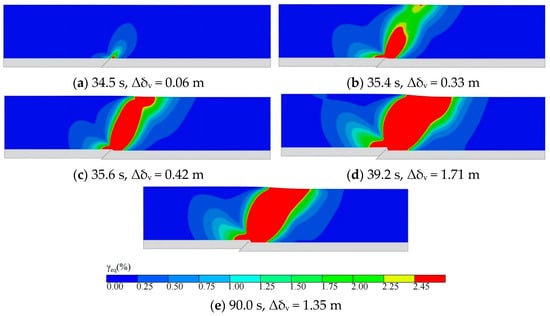
Figure 11 illustrates the evolution of equivalent shear strain in the overlying soil layer under dynamic reverse-fault displacement. Rupture initiates at the base of the soil layer at 34.5 s, corresponding to a fault vertical displacement (Δδv) of 0.06 m (Figure 11a). Surface rupture emerges at 35.4 s (Δδv = 0.33 m; Figure 11b), and the rupture zone becomes fully connected at 35.6 s (Δδv = 0.42 m; Figure 11c). The rupture area reaches its maximum extent at 39.2 s, as the fault displacement peaks at 1.71 m (Figure 11d). By 90.0 s (Δδv = 1.35 m; Figure 11e), some deformation recovery is observed in the overlying soil. It should be noted that the deformation patterns and strain localizations shown in Figure 11 (and the subsequent figures) are obtained from an idealized numerical model intended for mechanism-oriented comparison, rather than for direct matching to the detailed geometry of a particular near-fault soil site.
Figure 11.
Dynamic simulation: equivalent shear strain contours for the reverse fault. Panels (a–e) correspond to successive rupture stages: (a) rupture initiation, (b) surface rupture emergence, (c) rupture fully connects, (d) peak fault displacement, and (e) final state of the simulation.
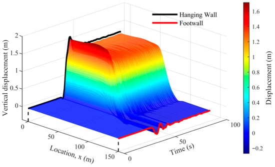
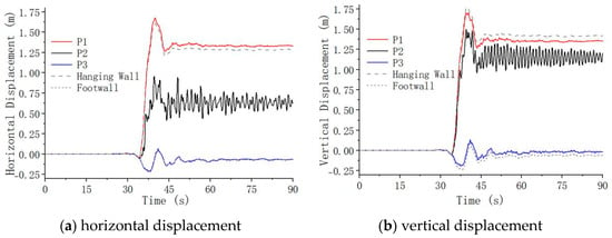
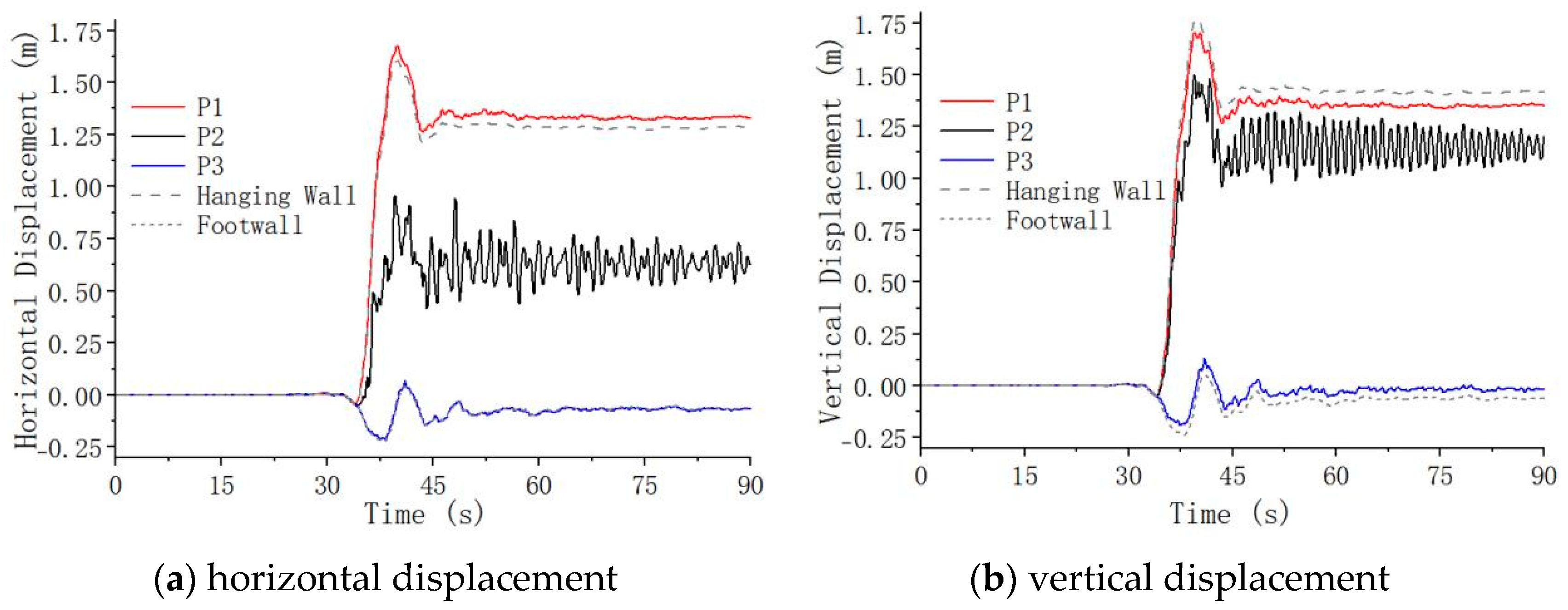
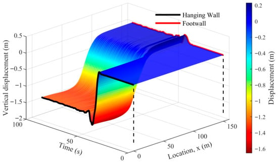
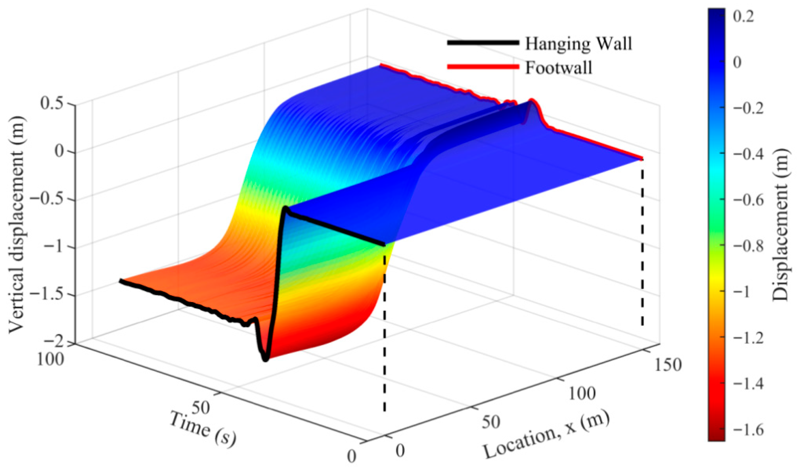
To reveal the spatiotemporal evolution of surface deformation, Figure 12 presents the three-dimensional trajectories of surface nodes, while Figure 13 shows the displacement time histories at three representative surface points: P1 (X = 30 m) on the hanging wall, 30 m left of the fault; P2 (X = 75 m) in the surface rupture zone, 15 m right of the fault; and P3 (X = 120 m) on the footwall, 60 m right of the fault.
Figure 12.
Surface displacement trajectories for the reverse fault. The dashed lines are included as visual guides to indicate the reference positions along the location axis in the 3D plot.
Figure 13.
Displacement time histories at typical surface points.
Analysis of the surface trajectories (Figure 12) and displacement time histories (Figure 13) reveals complex relative motion across the fault during shaking, with the maximum relative displacement typically occurring transiently rather than in the final deformed state. The dynamic simulation successfully captures the time-varying displacement trajectories of surface points, enabling accurate identification of key parameters such as peak displacement and maximum offset. Notably, the displacement time history at point P2, located within the rupture zone, exhibits significant oscillation. This oscillatory response arises from the superposition of non-uniform wave inputs from the two sides of the fault within this zone. Furthermore, the absence of an energy dissipation mechanism in the adopted nonlinear elastic constitutive model contributes to the slow decay of these oscillations.
Comparing the dynamic simulation results with the quasi-static analysis in Section 3.2 reveals both similarities and differences in soil response. In terms of rupture development, the fault vertical displacements required for surface rupture initiation and full penetration in the dynamic analysis are 0.33 m and 0.42 m, respectively, which are essentially consistent with the quasi-static results (0.35 m and 0.41 m). This suggests that the initiation and progression of shear rupture in the soil are primarily governed by the accumulated fault displacement, with the dynamic nature of fault displacement itself having no significant accelerating effect on soil rupture development. This behavior can be explained by the adopted rupture criterion, in which rupture extension is identified by reaching a prescribed critical shear strain threshold (Section 2.1.2). Under the nonlinear elastic constitutive formulation used here (without viscous or hysteretic components), dynamic shaking does not induce cumulative damage; therefore, the displacement threshold for rupture is mainly controlled by the geometric offset and the resulting accumulation of shear deformation.
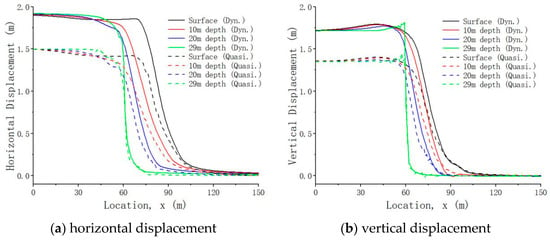
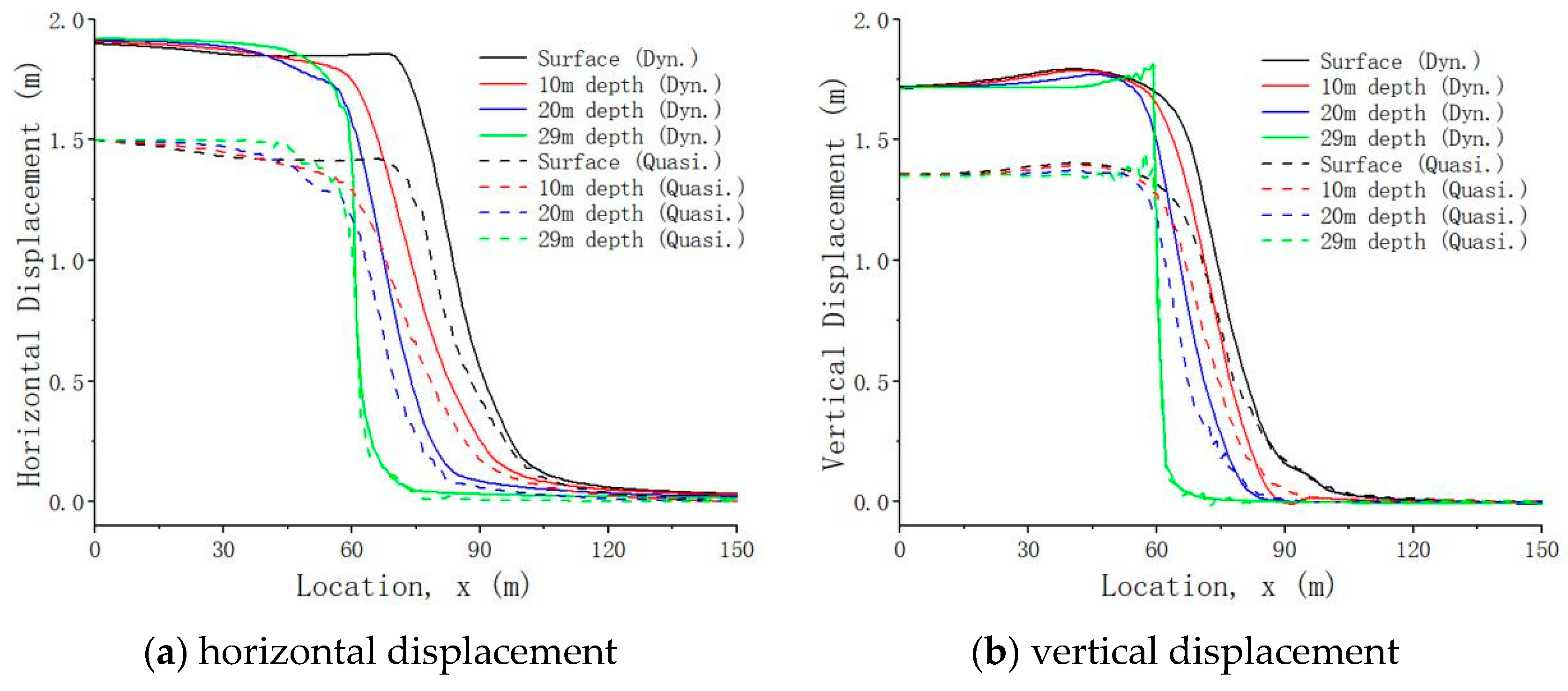
Analysis of the soil deformation response reveals a critical limitation of the quasi-static approach. The dynamic simulation predicts a significantly larger peak surface displacement than the quasi-static analysis (Figure 14). The results show that reverse faulting under dynamic loading produces concentrated uplift on the hanging wall and a distinct, localized shear band. These features are accompanied by pronounced transient deformation and oscillation that are not captured by quasi-static analysis.
Figure 14.
Displacement profiles for the reverse fault: dynamic vs. quasi-static analysis. Dynamic results correspond to the instant of peak fault displacement, while quasi-static results represent the final loading stage. Positive vertical displacement indicates upward movement.
Notably, even the quasi-static analysis shows that surface horizontal displacement (approximately 1.5 m) exceeds the fault displacement (1.35 m) under reverse faulting, indicating that the compressive mechanism has induced pronounced thrust uplift. The dynamic analysis reveals a similar ratio between surface displacement (approximately 1.9 m) and peak fault displacement (1.7 m). However, this peak surface displacement is attained instantaneously under inertial forces, representing a fundamentally different loading path. This dynamic loading triggers a more intense soil response characterized by transient deformation concentration and sustained oscillation—a dynamic instability process that cannot be captured by quasi-static methods.
In summary, while shear rupture propagation in soil is primarily governed by accumulated static displacement, with limited influence from the dynamic process, the dynamic simulation provides crucial insights into the transient rupture propagation. It accurately reproduces the instantaneous dynamic amplification and instability phenomena induced by inertial forces, thereby offering a more comprehensive basis for seismic risk assessment in near-fault regions.
4.2. Normal Fault Dynamic Simulation
To provide a kinematically symmetric counterpart to the reverse fault case and complete the comparative analysis, this section examines rupture propagation during normal fault displacement.
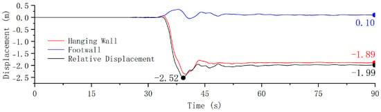
This example examines rupture propagation through a 30 m thick overlying soil layer during normal fault displacement. The input ground motion was derived by reversing the displacement time history used in the reverse fault simulation (Figure 15). The resulting peak relative fault displacement is −2.52 m (vertical component: −1.71 m), with a final displacement of −1.99 m (vertical component: −1.35 m).
Figure 15.
Input displacement time history for the normal fault case.
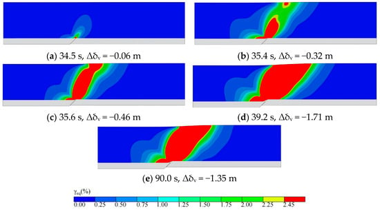
Figure 16 illustrates the rupture evolution under normal fault action. Rupture initiates at the base of the soil layer at 34.5 s, corresponding to a fault vertical displacement of −0.06 m (Figure 16a). Surface rupture emerges at 35.4 s (Δδv = −0.32 m; Figure 16b), and the rupture zone becomes fully connected at 35.7 s (Δδv = −0.46 m; Figure 16c). The rupture area reaches its maximum extent at 39.2 s, as the fault displacement peaks at −1.71 m (Figure 16d). By 90.0 s (Δδv = −1.35 m; Figure 16e), partial deformation recovery is observed in the overlying soil.
Figure 16.
Dynamic simulation: equivalent shear strain contours for the normal fault. Panels (a–e) correspond to successive rupture stages: (a) rupture initiation, (b) surface rupture emergence, (c) rupture fully connects, (d) peak fault displacement, and (e) final state of the simulation.
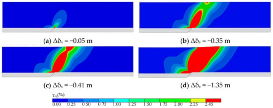
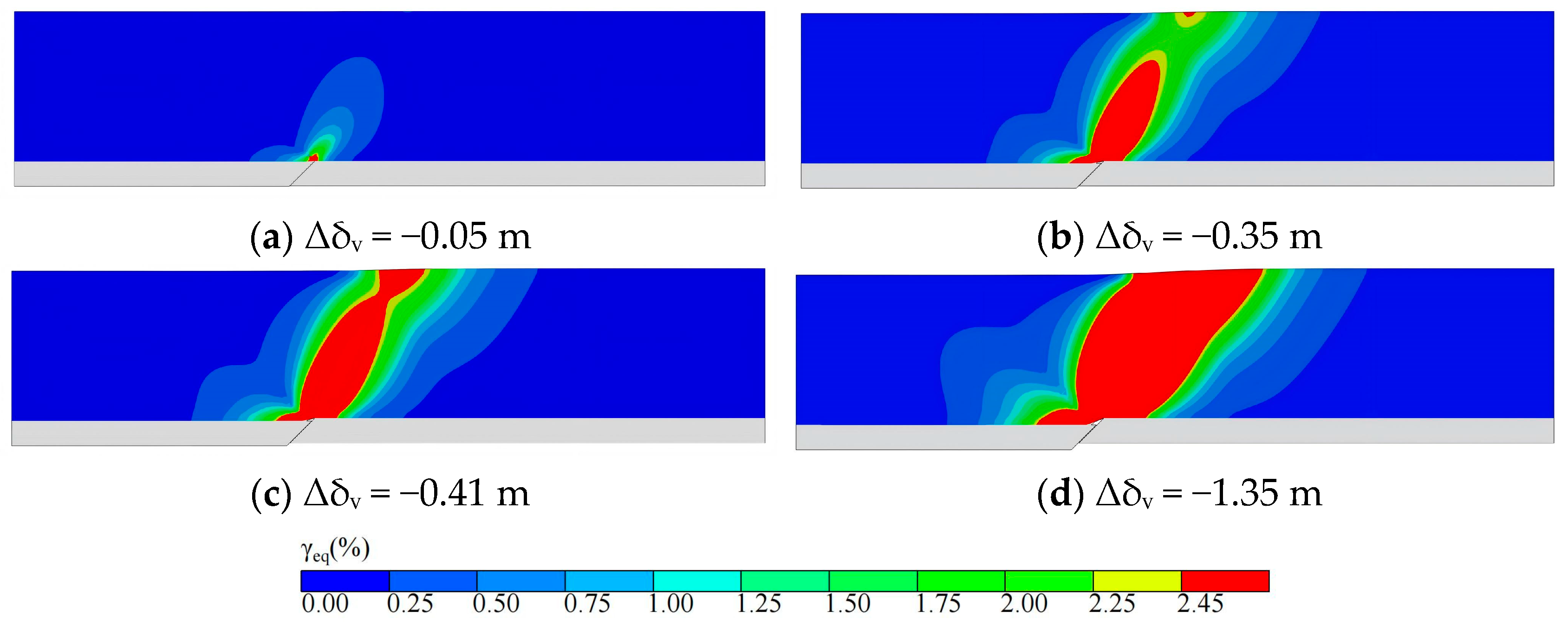
For comparison, a quasi-static simulation was conducted using the final fault displacement from the dynamic analysis as input. The resulting rupture propagation is shown in Figure 17: rupture begins at the soil base at a fault displacement of −0.05 m (Figure 17a), reaches the surface at −0.35 m (Figure 17b), and becomes fully continuous at −0.41 m (Figure 17c). The fault displacements required for rupture initiation and penetration in the dynamic and quasi-static analyses are closely aligned, further supporting the conclusion that the amount of fault displacement required to induce soil rupture is largely independent of the loading method under the adopted rupture criterion and constitutive formulation.
Figure 17.
Quasi-static simulation: equivalent shear strain contours for the normal fault. Panels (a–d) correspond to successive rupture stages: (a) rupture initiation, (b) surface rupture emergence, (c) rupture fully connects, (d) final state of the simulation.
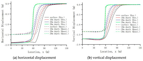
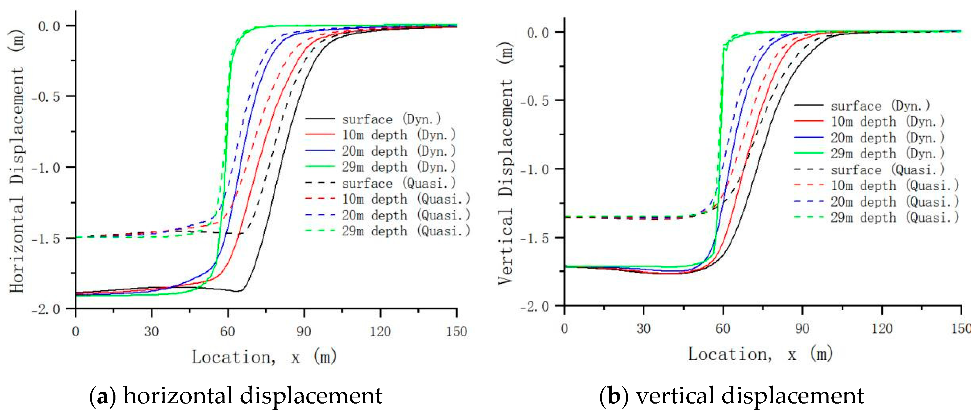
The dynamic simulation consistently demonstrates its superiority in capturing transient maximum deformation, as evidenced by the significantly larger peak displacements at all depths compared to the quasi-static results in the normal fault case (Figure 18).
Figure 18.
Displacement profiles for the normal fault: dynamic vs. quasi-static analysis. Dynamic results correspond to the instant of peak fault displacement, while quasi-static results represent the final loading stage. Positive vertical displacement indicates upward movement.
A comparison between Figure 14 and Figure 18 indicates that, the displacement fields induced by normal and reverse faulting show opposite overall patterns, consistent with the reversed slip direction. Accordingly, at each depth, the displacement profiles obtained from both quasi-static and dynamic analyses generally follow the imposed fault-displacement trend, while the dynamic solution captures transient maximum displacements.
The spatiotemporal evolution of surface motion for the normal fault (Figure 19) shows an overall pattern opposite in sense to that for the reverse-fault case (Figure 12), which is consistent with the kinematically symmetric fault displacement inputs in the two cases.
Figure 19.
Surface displacement trajectories for the normal fault.
In contrast, a comparison of the equivalent shear strain contours in Figure 11 and Figure 16 shows that, at comparable representative stages, the deformation zones within the overlying soil layer have broadly similar lateral extents, whereas their shapes are not identical. These differences are mainly reflected in the geometry of the high-strain regions, suggesting that the deformation of the soil is influenced by the distinct loading conditions and stress paths associated with normal-faulting and reverse-faulting scenarios.
This direct comparison between the two faulting mechanisms with opposite slip sense helps to clarify the role of dynamic analysis. While quasi-static methods correctly reproduce the overall deformation tendency (uplift versus settlement) and capture the final equilibrium configuration under both faulting scenarios (Figure 14), they ultimately present only a time-independent, static equilibrium snapshot. By contrast, the dynamic simulation resolves the full temporal evolution of ground deformation during fault loading, including physical processes that cannot be captured within a quasi-static framework. In particular, it reveals transient maximum displacement (Figure 12 and Figure 19) and sustained oscillatory responses (Figure 13) within the rupture zone driven by inertia and wave propagation.
Consequently, this study provides new physical insight by demonstrating that the core necessity of the dynamic method lies not in discovering fundamentally different failure modes, but in capturing the soil response associated with different fault mechanisms and the complete transient path leading to the final displaced configuration. This provides a richer and physically more comprehensive basis for evaluation of seismic effects than static equilibrium analysis alone.
5. Conclusions
This study has developed a comprehensive simulation methodology for modeling the complete process of rupture initiation and rupture propagation in overlying soil layers subjected to dynamic fault displacement. The approach integrates a nonlinear elastic constitutive model that captures soil nonlinearity and shear failure with a non-uniform wave input technique based on viscoelastic artificial boundaries. Implementation through a user-defined VUMAT subroutine in ABAQUS successfully reproduces the nonlinear stress–strain relationship and shear failure behavior of soil. The necessity and superiority of this dynamic approach were rigorously validated through a deliberate symmetric comparison at the kinematic level between the two fundamental, kinematically opposite faulting modes—normal (extensional) and reverse (compressional)—implemented using an identical model with opposite fault-slip directions.
Comparative analysis with quasi-static results demonstrates that while the fault displacement required for soil rupture initiation and penetration remains consistent across different analytical methods, the dynamic simulation uniquely captures transient soil displacement peaks and complete dynamic soil response processes unavailable through quasi-static analysis. Under reverse faulting, both quasi-static and dynamic analyses indicate pronounced uplift on the hanging-wall side. The dynamic analysis further shows that the maximum surface displacement is attained transiently during the loading process and is accompanied by sustained oscillations within the rupture zone due to the superposition of non-uniform wave inputs from the two sides of the fault. For normal faulting, the overall displacement pattern reverses consistently with the opposite slip direction, while the dynamic simulation still captures transient maximum displacements that cannot be obtained from quasi-static analysis. Moreover, although the two cases use kinematically opposite inputs, the high-strain zones exhibit broadly similar lateral extents but non-identical shapes, indicating different deformation characteristics under the two faulting mechanisms.
The simulation method developed in this study has two main limitations. Firstly, it requires spatial consistency between the incident seismic-wave direction and the fault-dip orientation, which arises from the assumptions adopted in the non-uniform input scheme. Secondly, because the method employs a nonlinear elastic constitutive model, the soil retains load-bearing capacity after reaching the strain criterion for failure. Consequently, if fault displacement continues to increase after rupture penetration through the soil layer, the subsequently computed surface deformation-band width may be overestimated.
Apart from these limitations, the proposed method is theoretically applicable to analyses of deformation, rupture, and dynamic response of overlying soils induced by various dipping faults, including both normal and reverse faulting, and can also be extended to non-horizontally layered sites or sites containing pre-existing fractures. In particular, because rupture is identified based on a shear-strain threshold within a nonlinear elastic framework, the method is more suitable for evaluating the potential extent of rupture influence and the overall deformation characteristics of the near-fault soil mass, rather than for precisely predicting the detailed locations and geometries of primary and secondary rupture bands.
In summary, this study has established a dynamic numerical analysis method capable of effectively simulating the rupture propagation in overlying soil layers under dynamic fault displacement. The proposed methodology captures essential dynamic features—including wave propagation and inertial effects—that remain beyond the reach of conventional quasi-static analysis. Validation and comparative analysis demonstrate that accounting for the dynamic nature of fault displacement is essential for accurate assessment of surface deformation extent, magnitude, and rupture zone characteristics. The methodology thus provides a more reliable basis for the seismic design of engineering projects crossing active faults.
Author Contributions
Conceptualization, C.W. and M.R.; methodology, C.W. and X.L.; software, C.W.; validation, C.W., M.R. and J.W.; formal analysis, C.W.; investigation, C.W. and K.C.; resources, M.R.; data curation, C.W. and K.C.; writing—original draft preparation, C.W.; writing—review and editing, M.R. and X.L.; visualization, C.W.; supervision, M.R. and X.L.; project administration, M.R.; funding acquisition, M.R. All authors have read and agreed to the published version of the manuscript.
Funding
This research was funded by the National Key Research and Development Program of China [2023YFC3007401].
Data Availability Statement
The strong ground motion records from the 1999 Chi-Chi earthquake used in this study were obtained from the Strong Motion Instrumentation Program operated by the Central Weather Bureau (CWB) of Taiwan. These data were accessed and downloaded in 2024 via the CWB’s online data repository (https://scweb.cwa.gov.tw/, accessed on 16 April 2024). The model parameters adopted in this study were derived from the work of Li et al. [25], as used for model validation in Section 3.2. The same set of parameters was subsequently applied to all case studies presented herein.
Conflicts of Interest
The authors declare no conflicts of interest. The funders had no role in the design of the study; in the collection, analyses, or interpretation of data; in the writing of the manuscript; or in the decision to publish the results.
References
- Tocher, D. Earthquake Energy and Ground Breakage. Bull. Seismol. Soc. Am. 1958, 48, 147–153. [Google Scholar] [CrossRef] [Scilit]
- Bonilla, M.G.; Mark, R.K.; Lienkaemper, J.J. Statistical Relations among Earthquake Magnitude, Surface Rupture Length, and Surface Fault Displacement. Bull. Seismol. Soc. Am. 1984, 74, 2379–2411. [Google Scholar]
- Wells, D.L.; Coppersmith, K.J. New Empirical Relationships among Magnitude, Rupture Length, Rupture Width, Rupture Area, and Surface Displacement. Bull. Seismol. Soc. Am. 1994, 84, 974–1002. [Google Scholar] [CrossRef] [Scilit]
- Xu, L.; Tian, H.; Jin, C.; Liu, H.; Wang, J.; Liu, W.; Xie, L. New Conditional Ground Motion Model for Permanent Displacement in Near-Fault Zones. Soil Dyn. Earthq. Eng. 2026, 200, 109774. [Google Scholar] [CrossRef] [Scilit]
- Deng, Q.; Yu, G.; Ye, W. Study on the Relationship Between Earthquake Surface Rupture Parameters and Magnitude (2); Seismological Press: Beijing, China, 1992. [Google Scholar]
- Ye, W.; Xu, X.; Wang, L. Quantitative Relationship between Surface Rupture Parameter, Earthquake Magnitude and Recurrence Interval for Surface-Rupturing Earthquakes in West China. Seismol Geol. 1996, 18, 37–44. [Google Scholar]
- Tie, R.; Wang, J.; Jia, L.; Guo, M. Data Statistics of Strong-Moderate Earthquake and Characteristics Research of Ground Rupture. World Earthq. Eng. 2016, 32, 112–116. [Google Scholar]
- Sanford, A.R. Analytical and Experimental Study of Simple Geologic Structures. Bull Geol. Soc. Am. 1959, 70, 19–52. [Google Scholar] [CrossRef] [Scilit]
- Emmons, R.C. Strike-Slip Rupture Patterns in Sand Models. Tectonophysics 1969, 7, 71–87. [Google Scholar] [CrossRef] [Scilit]
- Johansson, J.; Konagai, K. Fault Induced Permanent Ground Deformations—An Experimental Comparison of Wet and Dry Soil and Implications for Buried Structures. Soil Dyn. Earthq. Eng. 2006, 26, 45–53. [Google Scholar] [CrossRef] [Scilit]
- Johansson, J.; Konagai, K. Fault Induced Permanent Ground Deformations: Experimental Verification of Wet and Dry Soil, Numerical Findings’ Relation to Field Observations of Tunnel Damage and Implications for Design. Soil Dyn. Earthq. Eng. 2007, 27, 938–956. [Google Scholar] [CrossRef] [Scilit]
- Lee, J.W.; Hamada, M. An Experimental Study on Earthquake Fault Rupture Propagation through a Sandy Soil Deposit. Doboku Gakkai Ronbunshu 2005, 2005, 780_1–780_13. [Google Scholar] [CrossRef] [Scilit]
- Liu, X.; Hamada, M. Experiments on Rupture Propagation of Active Faults in Soil. Chin. J. Ceotech. Eng. 2004, 3, 425–427. [Google Scholar]
- Shi, J. Model Test and Numerical Study on the Destructions of Overlaying Soil and Tunnels by Faulting. Ph.D. Thesis, Zhejiang University, Hangzhou, China, 2019. [Google Scholar]
- Roth, W.H.; Scott, R.F.; Austin, I. Centrifuge Modeling of Fault Propagation through Alluvial Soils. Geophys. Res. Lett. 1981, 8, 561–564. [Google Scholar] [CrossRef] [Scilit]
- Bransby, M.F.; Davies, M.C.R.; Nahas, A.E. Centrifuge Modelling of Normal Fault–Foundation Interaction. Bull. Earthq. Eng. 2008, 6, 585–605. [Google Scholar] [CrossRef] [Scilit]
- Bransby, M.F.; Davies, M.C.R.; El Nahas, A.; Nagaoka, S. Centrifuge Modelling of Reverse Fault–Foundation Interaction. Bull. Earthq. Eng. 2008, 6, 607–628. [Google Scholar] [CrossRef] [Scilit]
- Guo, E.; Shao, G.; Bo, J.; Shi, Z. A Method for Earthquake Rupture Analysis of Overlying Soil Site. Earthq. Eng. Eng. Vib. 2002, 5, 122–126. [Google Scholar] [CrossRef]
- Shen, C.; Bo, J.; Qi, W.; Zhang, X.; Huang, J.; Qiao, F. Analysis of the Surface Rupture Process of Strong Earthquakes Based on Centrifuge Tests. Soil Dyn. Earthq. Eng. 2020, 136, 106239. [Google Scholar] [CrossRef] [Scilit]
- Shahidi, A.R.; Vafaeian, M. Analysis of Longitudinal Profile of the Tunnels in the Active Faulted Zone and Designing the Flexible Lining (for Koohrang-III Tunnel). Tunn. Undergr. Space Technol. 2005, 20, 213–221. [Google Scholar] [CrossRef] [Scilit]
- Bray, J.D.; Seed, R.B.; Ciuff, L.S.; Seed, H.B. Earthquake Fault Rupture Propagation through Soil. J. Geotech. Eng. 1994, 120, 543–561. [Google Scholar] [CrossRef] [Scilit]
- Bray, J.D.; Seed, R.B.; Seed, H.B. Analysis of Earthquake Fault Rupture Propagation through Cohesive Soil. J. Geotech. Eng. 1994, 120, 562–580. [Google Scholar] [CrossRef] [Scilit]
- Loukidis, D.; Bouckovalas, G.D.; Papadimitriou, A.G. Analysis of Fault Rupture Propagation through Uniform Soil Cover. Soil Dyn. Earthq. Eng. 2009, 29, 1389–1404. [Google Scholar] [CrossRef] [Scilit]
- Zanjani, M.M.; Soroush, A. Numerical Modeling of Reverse Fault Rupture Propagation through Clayey Embankments. Int. J. Civ. Eng. 2013, 11, 122–132. [Google Scholar]
- Zanjani, M.M.; Soroush, A. Numerical Modelling of Fault Rupture Propagation through Layered Sands. Eur. J. Environ. Civ. Eng. 2019, 23, 1139–1155. [Google Scholar] [CrossRef] [Scilit]
- Garcia, F.E.; Bray, J.D. Discrete Element Analysis of Earthquake Surface Fault Rupture through Layered Media. Soil Dyn. Earthq. Eng. 2022, 152, 107021. [Google Scholar] [CrossRef] [Scilit]
- Zhao, L. Study on Rupture Process of Overlaying Soil Due to Fault Bedrock Dislocation of Earthquake Fault and Its Effects on Buried Pipelines. Ph.D. Thesis, Institute of Geophysics, China Earthquake Administration, Beijing, China, 2004. [Google Scholar]
- Zhao, L.; Li, X.; Huo, D. Study on the Rupture Characteristics of Overlying Soil with Soft Interlayer on Bedrock under Fault Dislocation. Acta. Seismol Sin. 2006, 19, 563–568. [Google Scholar] [CrossRef] [Scilit]
- Li, X.; Zhao, L.; Li, Y. Simulation of Fault Movement Induced Rupture Process of Overlaying Soil of Bedrock. Chin J. Rock Mech. Eng. 2009, 28, 2703–2707. [Google Scholar]
- Zhao, Y.; Guo, E.; Wang, Q.; Liu, Z. Estimate Method of Dislocation to Seismic Surface Rupture under Strike-Slip Fault. Rock Soil Mech. 2013, 34, 1403–1408. [Google Scholar] [CrossRef]
- Zhang, B. Study on Response of Overlying Soil Against Dip-Slip Fault and Seismic Isolation Measure for Embankment. Master’s Thesis, Southwest Jiaotong University, Chengdu, China, 2012. [Google Scholar]
- Zhang, K.; Li, M.; Wang, Z. Dynamic Elastic-Plastic Models of Soils Based on Non-Mansing’s Rule. Earthq. Eng. Eng. Dyn. 1997, 17, 74–81. [Google Scholar]
- Chi, S.; Guo, X.; Yang, J.; Lin, G. Small Strain Characteristics and Threshold Strain of Dynamic Hardin-Drnevich Model for Soils. Chin. J. Ceotech. Eng. 2008, 2, 243–249. [Google Scholar]
- Dong, Q.; Chen, S.; Li, X.; Dong, Y.; Chen, Y.; Zhou, Z.; Zhu, J. Multi-Dimensional Implementation of Logarithmic Dynamic Skeleton Constitutive Model and Its Application in ABAQUS. Chin. J. Geotech. Eng. 2025, 47, 192–199. [Google Scholar] [CrossRef]
- Zhao, M. Stress-Type Time-Domain Artificial Boundary Condition for Finite-Element Simulation of near-Field Wave Motion and Its Engineering Application. Ph.D. Thesis, Beijing University of Technology, Beijing, China, 2009. [Google Scholar]
- Du, X.; Zhao, M.; Wang, J. Artificial Stress Boundary Conditions for Near-Field Wave Simulation. Chin. J. Theor. Appl. Mech. 2006, 1, 49–56. (in Chinese). [Google Scholar]
- Zhao, M.; Du, X.; Liu, J.; Han, Q. Time-Domain Method for Free Field in Layered Half Space under P—SV Waves of Oblique Incidence. China Earthq. Eng. J. 2013, 35, 84–90. [Google Scholar]
- Ma, S.; Chi, M.; Chen, H.; Chen, S. Implementation of Viscous-Spring Boundary in ABAQUS and Comparative Study on Seismic Motion Input Methods. Chin. J. Rock Mech. Eng. 2020, 39, 1445–1457. [Google Scholar] [CrossRef]
- Li, S.; Liu, J.; Bao, X.; Jia, Y.; Chen, Y.; Xiao, L. Implementation for Seismic Wave Input Method Based on the Artificial Boundary Substructure in ABAQUS. J. Nat. Disasters 2020, 29, 133–141. [Google Scholar] [CrossRef]
- Zhao, M.; Sun, W.; Gao, Z.; Huang, J.; Du, X. Input Method of Obliquely Incident Earthquake for Step-Shaped Layered Site. Eng. Geol. 2019, 36, 62–68. [Google Scholar]

Disclaimer/Publisher’s Note: The statements, opinions and data contained in all publications are solely those of the individual author(s) and contributor(s) and not of MDPI and/or the editor(s). MDPI and/or the editor(s) disclaim responsibility for any injury to people or property resulting from any ideas, methods, instructions or products referred to in the content. |
© 2026 by the authors. Licensee MDPI, Basel, Switzerland. This article is an open access article distributed under the terms and conditions of the Creative Commons Attribution (CC BY) license.