


Abstract
Transporting hazardous materials has low accident probabilities but potentially catastrophic consequences, making effective risk management essential in uncertain conditions such as population distribution, weather, traffic, and multimodal scheduling constraints. This study develops a Conditional Value-at-Risk (CVaR)-based optimization model for multimodal hazardous materials transportation that incorporates transportation and transshipment risks, population exposure uncertainty, fixed departure schedules for rail and waterway transport, dual time-window constraints, and limits on the number of transshipments. The model also reflects the decision-maker’s risk aversion and time-varying travel times. To solve this NP-hard problem, an improved chaotic simulated annealing-ant colony optimization (CSAACO) algorithm is proposed. Numerical experiments show that CSAACO outperforms the standard ACO in terms of solution quality and stability. The results demonstrate that the model effectively captures tail risk in dynamic environments and that both the risk aversion coefficient μ and departure time significantly influence route selection. The proposed approach provides an efficient and practical decision-support tool for hazardous materials multimodal transportation planning under uncertainty.
1. Introduction
Hazardous materials are essential to industrialized societies. Statistics indicate that in China alone, over 4 billion metric tons of hazardous materials are transported annually, with more than 95% requiring cross-regional shipment [1]. Although the probability of hazardous material transportation accidents is relatively low, these accidents often exhibit a “low-probability, high-consequence” profile. When such accidents occur, they can cause severe casualties, environmental pollution, and substantial property losses [2].
Existing research predominantly focuses on static network models aimed at minimizing cost or average risk, which fails to adequately capture the time-varying and uncertain nature of actual hazardous materials transportation. Given that factors such as population density and traffic conditions dynamically influence risk levels, and multimodal transport involves dual complex constraints—fixed schedules (departure time windows) and customer delivery requirements (arrival time windows)—traditional expected-risk models are no longer sufficient to characterize low-probability, high-consequence tail risks. To address this, this paper introduces Conditional Value-at-Risk (CVaR) as a risk measurement tool and constructs a time-varying path optimization model that incorporates dual time windows. To tackle this NP-hard problem, a hybrid chaotic simulated Annealing-ant colony optimization (CSAACO) algorithm is designed to enhance solution efficiency and global search capability. Through simulation and case studies, the effectiveness of the model and algorithm is validated, and the influence of the risk aversion coefficient and departure time on routing decisions is examined, thereby providing decision-making support for hazardous materials multimodal transport under uncertain conditions.
The structure of this paper is organized as follows: Section 2 provides a literature review, systematically examining research in the field of hazardous materials transportation, including route planning, multimodal transport optimization, and risk measurement methods employing Value-at-Risk (VaR) and Conditional Value-at-Risk (CVaR). Section 3 describes and formulates the hazardous materials multimodal transportation problem addressed in this study. Section 4 proposes a hybrid simulated annealing-ant colony optimization (CSAACO) algorithm for solving the proposed model. Section 5 conducts simulation experiments, analyzes the results, and validates the effectiveness of the model through a practical case study. Finally, Section 6 summarizes the research findings and suggests directions for future work.
2. Literature Review
Hazardous materials routing has attracted substantial scholarly attention. Mohri et al. [3] provided a comprehensive survey of research advances in hazardous material transportation problems. Du et al. [4] studied a multi-depot hazardous material vehicle routing problem (HMVRP) with the objective of minimizing expected risk, formulating a fuzzy bilevel integer programming model and developing four fuzzy heuristic algorithms for its solution. Ma et al. [5,6] investigated a multi-depot hazardous material transportation routing problem that considers both fuel consumption and transportation risk as optimization objectives. They employed a two-phase method to assign customers to distribution centers and solved the routing problem using a hybrid multi-objective genetic algorithm integrated with a genetic-algorithm- and neural-network-based screening strategy. Focusing on minimizing the maximum local risk in urban areas, Zhang et al. [7] proposed an optimization model that treats the hazardous material transportation service network as a key decision variable and solved it using a heuristic algorithm. Wang et al. [8] developed a multi-depot semi-open hazardous material vehicle routing model that incorporates customer relationships, with the objectives of minimizing total transportation cost, transportation risk, and total delay time; a hybrid ant colony optimization–simulated annealing (ACO–SA) nested algorithm was designed to solve the model. Shi et al. [9] proposed a hazardous material vehicle routing optimization model that accounts for time-varying risk and population exposure, capturing the dynamic characteristics of road transportation environments, with the objectives of minimizing total risk, total cost, and total vehicle travel time.
In response to low-carbon requirements, Ma et al. [10] studied a heterogeneous fleet hazardous material vehicle routing problem, jointly optimizing total transportation risk, total cost, and total carbon emissions in the context of explosive hazardous material transportation. A soft time window penalty function was introduced, and the non-dominated sorting genetic algorithm (NSGA) was improved in two aspects. Chai et al. [11] proposed a two-stage optimization framework for the hazardous material vehicle routing problem with time windows (HMVRPTW). Zhang et al. [12] constructed a hazardous chemical routing optimization model with a single distribution center and time window constraints, which was solved using a genetic algorithm. Wang et al. [13] addressed hazardous material distribution routing in urban environments by developing a dynamic, uncertain risk assessment framework and formulating a multi-objective, nonlinear optimization model that minimizes transportation risk, transportation cost, and carbon emissions under time-window and load-capacity constraints.
Considering both link risk and path risk, Wang et al. [14] investigated road transportation route optimization for hazardous goods and proposed a multi-objective model that minimizes total transportation cost, overall path risk, and the disparity between the maximum and minimum link risks, which was solved using an NSGA-III algorithm. Kuang et al. [15] examined the facility location and route selection problem for hazardous materials under continuous-time-varying risk, developing a nonlinear risk measurement model with dual objectives: minimizing total continuous-time-varying risk and total transportation cost. Zhang et al. [16], from both managerial and economic perspectives, formulated a multi-objective hazardous goods transportation routing model that prioritizes transportation risk while also considering cost and travel time, and designed a genetic algorithm for its solution. Finally, Wang et al. [17] investigated the hazardous materials vehicle routing problem under uncertainty by proposing a multi-objective optimization model that minimizes total transportation risk, total travel distance, and the number of vehicles subject to constraints on time windows, accident probability, and vehicle capacity.
As transportation infrastructure, such as highways, railways, and waterways, continues to improve, an increasing volume of freight is moved through intermodal transportation systems that exploit the complementary advantages of different transport modes. This development has attracted considerable scholarly attention. Liang et al. [18] examined the rail–road intermodal routing problem under demand uncertainty. Jia et al. [19] incorporated time-dependent characteristics, node transshipment time, transportation risk, and cost into hazardous materials rail–road intermodal transportation, formulating an integer programming model on a time–space network to minimize transportation risk and solving it using an improved Dijkstra algorithm. To address inequitable risk distribution across regions along transportation corridors, Li et al. [20] quantified regional risk equity through risk compensation costs, defined as the sum of en-route and transshipment risk compensation. Based on this measure, they developed an optimization model for hazardous materials rail–road intermodal routing that simultaneously minimizes transportation risk, risk compensation cost, and transportation expenditure, and proposed an ant colony optimization algorithm for its solution. Fang and Jia [21] proposed a multi-objective optimization model that jointly considers transportation cost and risk and designed an improved non-dominated sorting genetic algorithm (NSGA) to solve the model. Extending this line of research, Li et al. [22] investigated the hazardous materials rail–road intermodal network expansion problem over multiple planning periods. With the objectives of minimizing total cost and transportation risk, they established a mixed-integer probabilistic robust optimization model and solved it using a simulated annealing algorithm. Focusing on the transshipment process, He et al. [23] treated human, equipment, management, environmental, and transshipment-related factors as decision attributes and employed the TOPSIS method based on hesitant intuitionistic fuzzy linguistic sets to evaluate alternative intermodal transportation schemes.
As research on hazardous materials transportation route optimization has progressed, scholars have increasingly recognized that transportation risks vary substantially across hazardous materials categories and that decision-makers exhibit heterogeneous risk aversion preferences. Accordingly, incorporating decision-makers’ risk attitudes into hazardous materials transportation planning has become essential. Kang et al. [24] were among the first to introduce the Value-at-Risk (VaR) methodology—a classical risk measurement tool widely used in finance—into hazardous materials transportation risk assessment. They developed a VaR-based risk evaluation model tailored to hazardous materials transportation and demonstrated its effectiveness in accommodating the risk preference requirements of decision-makers with varying degrees of risk aversion. Building on this work, subsequent studies have extensively applied VaR in hazardous materials routing problems. Kang et al. [25] further integrated the VaR framework into hazardous materials route optimization in multi-trip and multi-hazard scenarios, with the objective of minimizing global VaR while satisfying equity constraints. Wang et al. [26] combined the VaR concept with fuzzy theory and proposed a Chance-Value-at-Risk (ChVaR) model based on chance measures, incorporating both probability and credibility measures to determine optimal routing schedules that minimize transportation risk under specified confidence levels. Recognizing that accident probabilities in hazardous materials transportation are influenced by multiple uncertain and stochastic factors, Wei et al. [27] applied VaR theory to construct a risk valuation model for hazardous materials transportation routes. Their model identifies the minimum-risk level of a hazardous-materials transportation network at a given confidence level, thereby yielding optimal routing schemes for different risk tolerance levels.
However, the VaR model evaluates only losses up to the VaR threshold and neglects tail risk beyond this value, limiting its ability to capture the potential impact of extreme events. Moreover, VaR lacks the property of subadditivity and therefore does not constitute a coherent risk measure. To overcome these shortcomings, Toumazis and Kwon [28] introduced Conditional Value-at-Risk (CVaR) theory into hazardous materials transportation and developed a CVaR-based route optimization model for road transportation under time-varying network conditions. Their model determines optimal transportation paths based on the decision-maker’s degree of risk aversion. By explicitly focusing on tail risk exceeding the VaR threshold, the CVaR framework aims to mitigate the consequences of low-probability but high-impact events, such as severe hazardous materials accidents. In addition, CVaR satisfies the axioms of a coherent risk measure and exhibits favorable mathematical properties for optimization. Building on this foundation, Faghih-Roohi et al. [29] proposed a CVaR-based route optimization model for single-mode hazardous materials transportation that incorporates time-varying risk and solved it using Dijkstra’s algorithm. He et al. [30] further considered the dynamic characteristics of hazardous material accident rates, road traffic density, and surrounding population density and developed a time-dependent CVaR-based routing model for road transportation. Extending CVaR applications to intermodal systems, Cao et al. [31] formulated a route selection model for hazardous materials rail–road intermodal transportation that accounts for decision-makers’ risk aversion. However, their model does not incorporate operational constraints such as schedule restrictions or limits on transshipment frequency; to solve the model, the intermodal network was transformed into a single-mode network and addressed using Dijkstra’s algorithm. In the context of railway transportation, Hosseini and Verma [32] incorporated equity considerations into a CVaR-based routing model and designed a k-shortest path algorithm for its solution. Similarly, Liu et al. [33] proposed a CVaR-based optimization framework for railway hazardous materials routing and developed a path selection algorithm based on k-shortest paths to balance extreme risk minimization with fair risk distribution. Table 1 summarizes the representative studies on CVaR-based hazardous materials route optimization.
Table 1.
Studies on CVaR-based hazardous material route optimization.
In summary, existing research has primarily focused on single-mode transportation, while the literature addressing route optimization for hazardous materials multimodal transportation remains relatively scarce. Furthermore, studies incorporating both destination time windows and the schedule constraints of railways or waterways (resulting in time window constraints at transshipment nodes)—i.e., dual time windows—along with CVaR in hazardous materials multimodal route optimization are even more limited. Regarding solution algorithms, given the NP-hard nature of the model, current research seldom employs ant colony algorithms for solving such problems. Therefore, this paper, considering the NP-hard characteristics of hazardous materials multimodal transportation, constructs a model incorporating mixed time windows and CVaR and designs an improved ant colony algorithm. This work holds both theoretical significance and practical application value.
3. Optimization Model
3.1. Problem Description
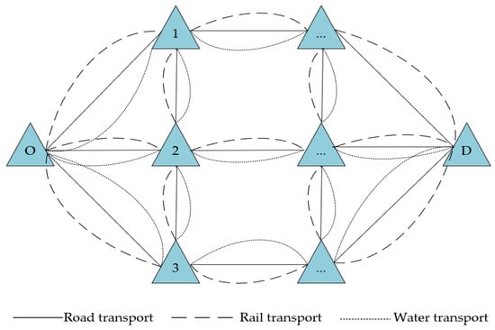
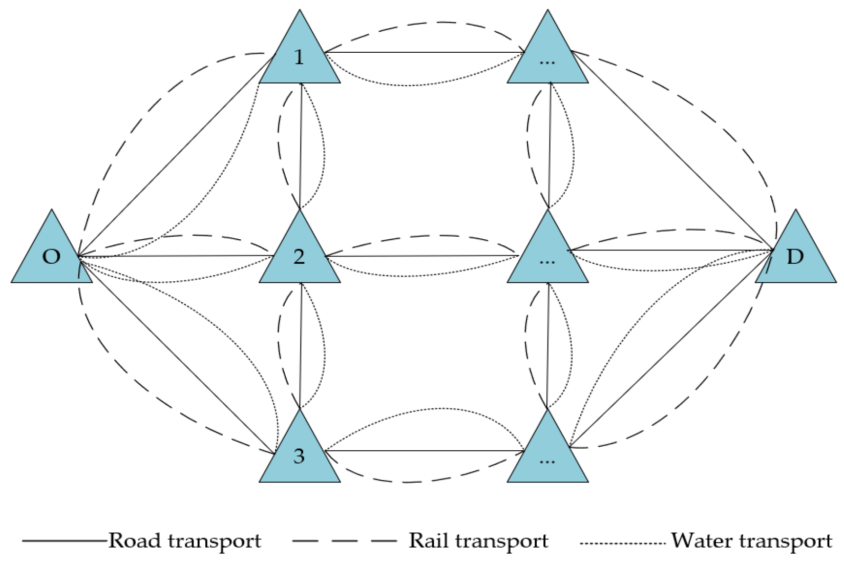
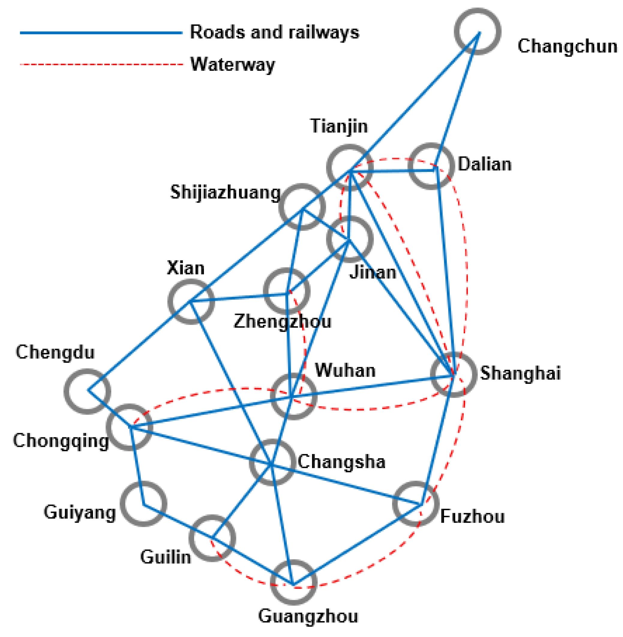
Within the hazardous materials multimodal transport network depicted in Figure 1, a shipment must be transported from origin O to destination D. Railway and waterway transport operate on fixed schedules. Given the time-varying nature of factors such as transport speed, population density along routes, and accident probabilities, the lowest-risk transport path and its departure time are to be determined at a specified confidence level. This path must deliver the hazardous materials to destination D within the stipulated time windows and in accordance with the transfer operation constraints. Some of the parameters and their meanings are shown in Table 2, Table 3 and Table 4.
Figure 1.
Multimodal transport network diagram.
Table 2.
Parameter definitions.
Table 3.
Set definitions.
Table 4.
Decision-making variables.
3.2. Travel Time Computation for Road Segments
In a time-varying network, the required travel time for a road segment varies with the arrival time. Because time-varying networks must satisfy the First In First Out (FIFO) rule, and Erkute [35] demonstrated that the time-dependent travel speed model adheres to the FIFO principle, the segment travel time is calculated using a piecewise travel speed model. Xi et al. [36] also investigated the route optimization problem for intra-city freight transportation, considering time-varying speed characteristics. Therefore, let the travel speed of mode m during the k time period be denoted as (k = 1, 2, … K) speed, and the distance of segment (i, j) as . If the departure time from node i is ti, the corresponding time period k can be determined by solving the following Equations (1) and (2) jointly.
Calculate the required travel time for entering the segment during this time period. Notably, travel time on a segment may fall into one of three scenarios: no cross-period travel, partial cross-period travel, and full cross-period travel.
- If (the travel does not span across time periods)
- 2.
- If and , (the travel time spans across time periods)
- 3.
- If none of the above conditions hold (i.e., the travel fully spans across multiple time periods), let the number of time periods required to be crossed be denoted as N (N = 0, 1, …, K−k). Combining Equations (11) and (12) yields N such that
The travel time can be further obtained as follows.
3.3. Time-Varying Conditional Value-at-Risk (TV-CVaR) Model
3.3.1. Conditional Value-at-Risk (CVaR)
- Risk Value Calculation
In hazardous materials transport route optimization, the primary task is to determine a method for quantifying risk. Common approaches include the average-variable model, the population-exposure model, and the TR model, among others. Among these, the TR model—during route computation—terminates the current route upon detecting danger and searches for alternative routes, thereby reducing the probability of accidents. Based on the TR model, this paper constructs a risk valuation model. The TR model uses the expected value of accident consequences across road segments as the route-level transportation risk metric, accounting for both accident likelihood and severity. Assume the probability of an accident occurring on a transport segment is , with the accident consequences denoted as . This study employs population
risk and affected zones to assess accident consequences. The probability of an accident
at a node is , with accident consequences . Assume the radius
of the affected area is r, as shown in Figure 2 below. The calculation of accident probability and consequence severity for road
segments and nodes is as follows:
Figure 2.
r radius and affected area: (a) affected area during transportation; (b) affected area in the transshipment center.
In the formula: π is the pi constant; is the arc length (m); is the average population density along the arc (persons/m2); is the average population density when
transferring from transport mode m to n at node j.
- 2.
- Conditional Value-at-Risk (CVaR) Model
Value-at-Risk (VaR) estimates the maximum potential loss likely to be incurred at a specific confidence level. It helps investors or managers assess potential risks for effective risk management [24]. In this context, the combination of road segments between an origin (O) and a destination (D) can be viewed as a financial investment portfolio, where the path that minimizes potential loss is considered the optimal route. For a given network G (N, A), the minimum value of β such that the probability of the risk value of path l not exceeding the risk threshold β is greater
than or equal to µ. The expression for the VaR of path l, denoted
as is given by
where µ represents the confidence level acceptable to the decision-maker. is the minimum value among all feasible paths, i.e.,
In the formula, denotes the risk value of the path with the minimum Value-at-Risk, and L represents the set of all feasible paths.
Considering a network composed of a set of hazardous materials transportation routes as the research object, it is assumed that each route consists of an ordered set of arcs , where denotes the k-th arc of the route. The accident consequences for all segments on each route are sorted in ascending order. Let represent the k-th smallest value in the set of accident consequences , and define . Let denote the accident probability corresponding to . The accident risk of the route is then determined using the corresponding probability values as follows:
In the expression, represents the cardinality of set , i.e., . Thus, the cumulative risk distribution probability can be derived as follows:
In Equation (15), represents the damage caused by an accident, where . Based on and the cumulative distribution function of , the Value-at-Risk for route at confidence level µ can be derived as follows:
Building upon , the Conditional Value-at-Risk (CVaR) for a given path l is defined by Kwon et al. [28] as
Since it is difficult to obtain and its integral in a closed form [28], minimizing is equivalent to
Given that the risk in hazardous materials multimodal transport comprises transportation risk, transfer risk, and waiting risk, minimizing can be equivalently expressed as
In the formula, τ represents VaR at the confidence level µ, and .
3.3.2. CVaR Model Under Time-Varying Conditions
In this study, one day is divided into two time periods, and . Due to variations in environmental conditions across time periods, the accident consequences, accident probabilities, and travel speeds within each period differ. Let the accident consequences and accident probabilities for transport mode m on segment (i, j) during periods and be denoted as , and , , respectively. Furthermore, assume that the waiting accident consequence and waiting accident probability Pw at node j are linearly related to the waiting time, yielding
In the formula, the first line represents the accident consequence and the corresponding accident probability when traversing road segment (i, j) during transportation; the second line represents the waiting accident consequence and the corresponding accident probability at transfer node j; and the third line represents the accident consequence and the corresponding accident probability at transfer node j.
The Conditional Value-at-Risk model under time-varying conditions is then formulated as
In the formula, represents the VaR under time-varying conditions, .
3.4. Hazardous Materials Multimodal Transport Routing Optimization Model
The constraint conditions are as follows: Equation (24) enforces flow conservation, specifying a net flow of +1 at the source node and −1 at the sink node, with all intermediate nodes maintaining flow equilibrium. Equation (25) restricts delivery arrival times to designated time windows. Equation (26) imposes a limit on the maximum allowable transfer operations. Equation (27) mandates that hazardous goods transportation between any two adjacent nodes must use a single transport mode. Equation (28) limits transfers to at most one operation per node. Equations (29) and (30) define binary decision variables constrained to {0, 1} values.
4. Algorithm Design
The multimodal transportation route optimization problem is NP-hard. The ant colony optimization (ACO) algorithm is more feasible for solving such problems than exact solution algorithms and has been widely applied. Ahmed et al. [37] addressed the NP-hard capacitated vehicle routing problem (CVRP) by proposing several variants of the ant colony optimization algorithm, introducing improvements to the algorithm, and ultimately demonstrating their effectiveness.
Consequently, this study proposes an enhanced chaotic simulated annealing-ant colony optimization algorithm (SA-ACO) to solve the problem.
4.1. Enhanced Chaotic Simulated Annealing-Ant Colony Optimization Algorithm
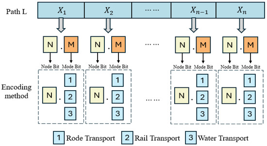
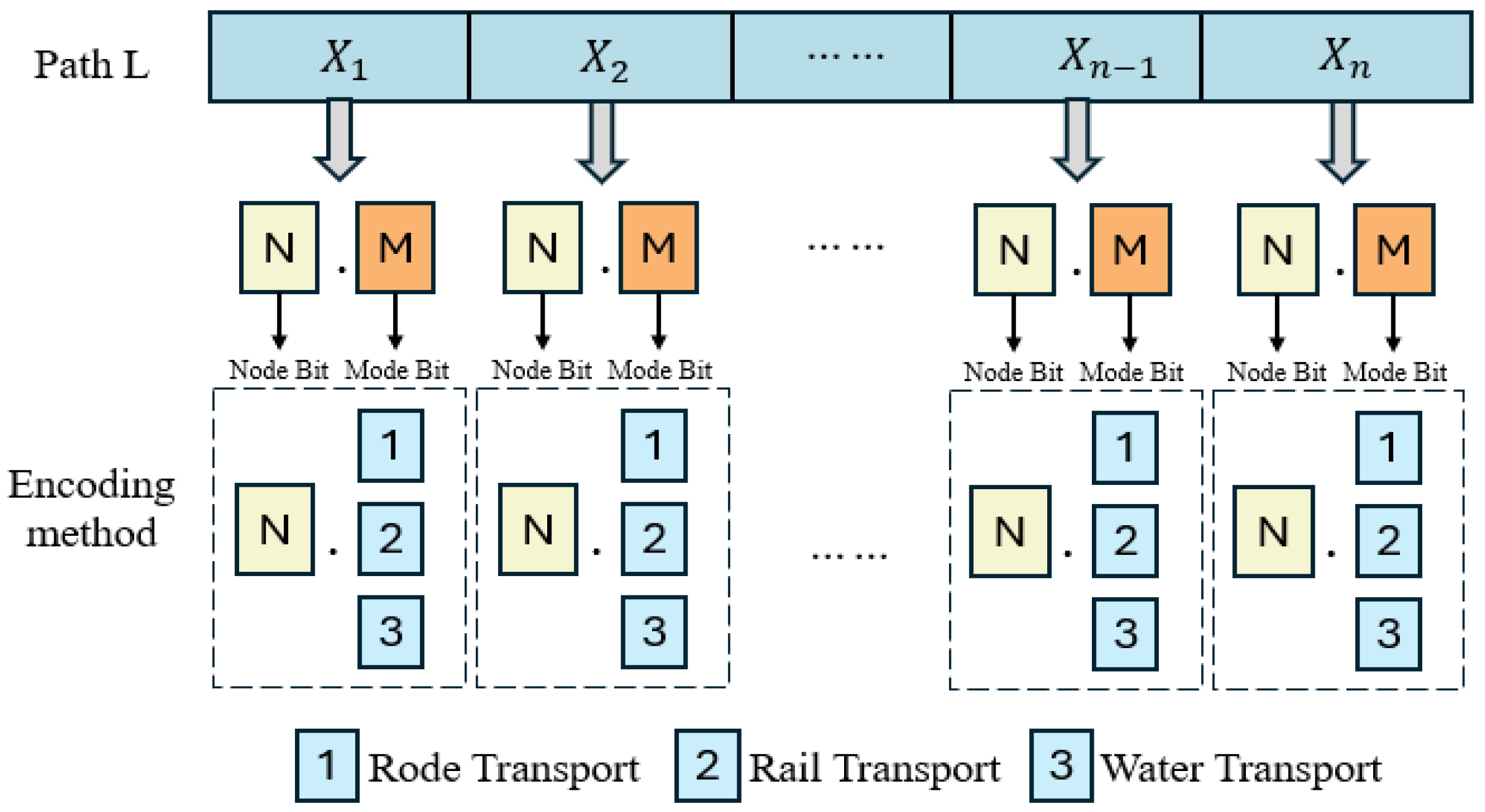
The multimodal transport routing optimization problem distinguishes itself from single-mode routing optimization by requiring not only the determination of node sequences along the path but also the specification of transport mode sequences between nodes. In multimodal networks, adjacent node pairs are connected by multiple transport modes. This study employs a decimal encoding scheme where
- 1 denotes Road transport
- 2 represents Rail transport
- 3 signifies Water transport
Figure 3 illustrates this decimal encoding methodology for inter-node mode selection.
Figure 3.
Transport mode encoding scheme.
Within ant colony optimization algorithms, the coexistence of positive and negative feedback mechanisms often traps ants in local optima, hindering the discovery of globally optimal paths and inducing premature convergence. To address this limitation, this study introduces a chaotic mapping for pheromone initialization, integrated with a simulated annealing mechanism, to prevent premature convergence while accelerating convergence. The methodology comprises two key innovations: first, pheromone distributions are initialized using a Logistic chaotic mapping to ensure search-process diversity; second, after each iteration, new solutions are generated based on optimal paths, and a directed perturbation strategy is applied—randomly selecting one pair of adjacent nodes within the optimal path and altering their transport mode encoding (1: Highway, 2: Railway, 3: Waterway) while preserving all other nodes’ configurations and the overall path topology.
4.2. Algorithmic Solution Process
- Integrate chaotic mapping for pheromone initialization
To prevent ants from converging to local optima, a chaotic perturbation is introduced to accelerate algorithm convergence. During pheromone initialization, the Logistic chaotic mapping method is used. The Logistic chaotic mapping equation is as follows:
where is the chaotic variable and µ is the control parameter.
When µ = 4 and , the system represented by the equation is in a chaotic state. The Logistic chaotic mapping is incorporated into the initialization of the pheromone as follows:
In the formula, is the pheromone evaporation coefficient, is the increment of pheromone quantity on path (i, j) in
this cycle, is the residual pheromone amount deposited by the k-th ant on
path (i, j) in the current cycle, and is an adjustable parameter.
- 2.
- Simulated Annealing Procedure
The enhanced chaotic simulated annealing-ant colony optimization algorithm operates as follows: After all ants complete a cycle, a new solution is generated based on the current optimal path. The generation strategy randomly selects one pair of adjacent nodes on this path and alters the transport mode between them while keeping all other nodes and the overall path topology unchanged. Following the principles of simulated annealing and the Metropolis criterion, the next step is to stochastically decide whether to accept this new path as the current optimal solution. The temperature parameter, which controls this acceptance probability, decays with the iteration count within the range [Tmin, Tmax]. The initial temperature is set to T(0) = Tmax.
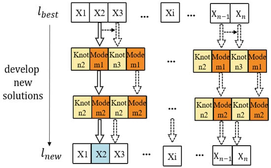
In the simulated annealing operation for generating new solutions, the strategy is as follows: Starting from the optimal solution of the current iteration found by the ants, denoted as , a single path node is randomly selected from those traversed at . The decimal part (transport mode encoding) of this node is evaluated to
determine if alternative transport modes are available. If other modes exist,
the current transport mode is changed to . This applies a random perturbation to the initial solution, generating
a new solution . The CVaR calculated from this new solution set is , as illustrated in Figure 4.
Figure 4.
Diagram of new solution generation via simulated annealing.
The difference in the objective function value is given by
To determine whether to accept the new solution as the current solution: if , accept the new solution; otherwise, accept it with the following probability:
Generate a uniformly distributed random number within the interval (0, 1). If , accept the new solution, making it the current optimal solution . Otherwise, retain the original solution, and the current optimal solution remains . After completing one cycle and updating the pheromone, cool down the temperature using the formula , where α is the cooling coefficient and .
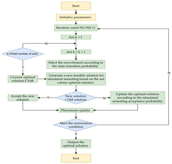
The particular procedure is depicted in Figure 5:
Figure 5.
Flowchart of the ant colony algorithm.
The hybrid algorithm begins by initializing all parameters. In each iteration, ants construct solutions using transition probabilities. A new solution is then generated from the ant colony’s best solution using a simulated annealing operator and is accepted based on a probabilistic criterion. The pheromone trails are updated globally after each iteration. This process repeats until a termination condition is met, at which point the optimal solution is output.
5. Calculation Analysis and Discussion
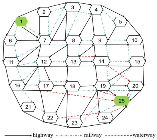
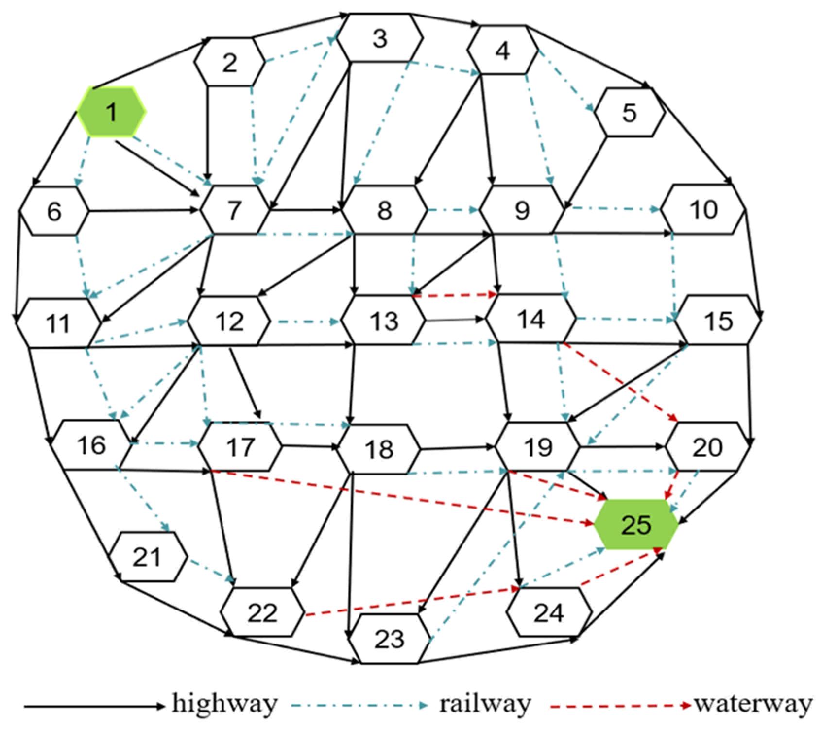
To validate the effectiveness of the proposed algorithm and model, it is assumed that a batch of hazardous goods with a total weight of Q = 40 t must be transported from the origin to the destination in accordance with enterprise requirements. The hard time window for delivery arrival is set as [Tmin, Tmax] = [60 h, 70 h], with a maximum of four transfers allowed. The multimodal transport network is illustrated in Figure 6, where nodes 1 and 25 represent the origin and destination, respectively. In this study, the first 25 points from the Solomon R101 benchmark instance are selected, corresponding to the nodes’ coordinates in the graph [38]. The distances between nodes are scaled by factors of 20, 10, and 10 for highway, railway, and waterway transport, respectively (in kilometers).
Figure 6.
Multimodal transport network diagram.
Speeds for different transport modes during the two time periods [7:00, 19:00] and [19:00, 7:00], as well as railway and waterway schedules, are provided in Table 5. Time-varying accident probability coefficients and population densities for different transport modes are listed in Table 6, as defined in Harwood et al. [39]. Transfer accident consequences, probabilities, and transfer times are presented in Table 7.
Table 5.
Speeds and schedules of different transport modes.
Table 6.
Time-varying accident probability coefficients and population density under different transport modes.
Table 7.
Transfer accident consequences, probabilities, and transfer times: H, Highway; R, Railway; W, Waterway.
5.1. Algorithm Comparison
For the case study above, this paper employs the previously proposed algorithm to find a solution. The algorithm is implemented in MATLAB 2021b. By considering different values of the decision-maker’s risk aversion level µ and accounting for time-varying factors during transportation, the model solves for the transport route and modes that minimize the transportation risk of hazardous goods between the origin and destination.
To investigate the impact of different risk aversion levels (µ) on optimal path selection, and based on fundamental ant colony algorithm parameters set as (α = 4), (β = 4), (), number of ants (m = 50), and iterations = 200, different values of µ and different departure times are configured to compare the optimal routes under these varying conditions.
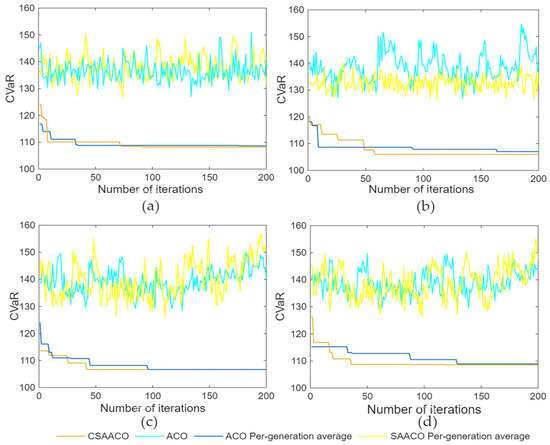
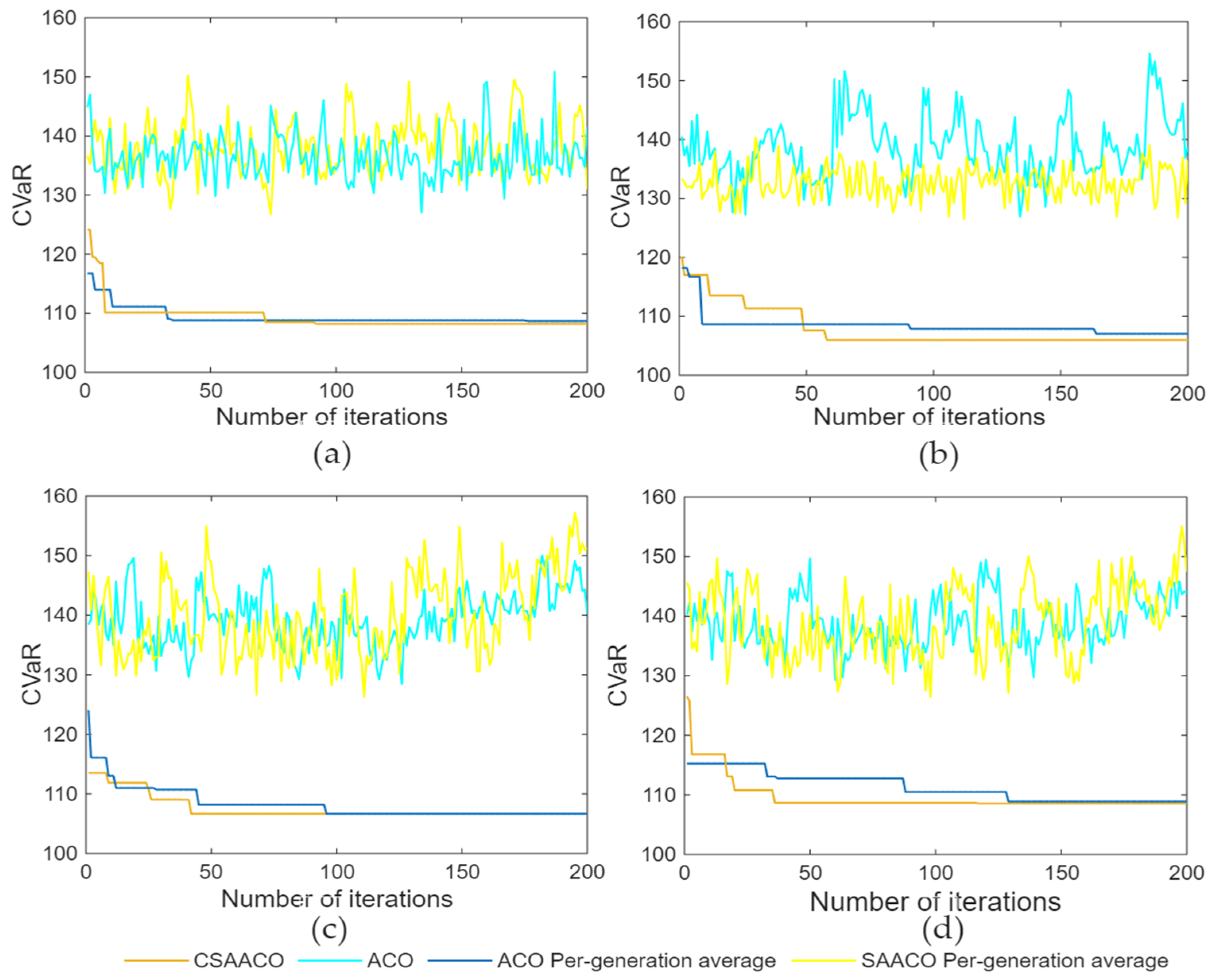
The optimization iteration process of the two algorithms under different departure times is illustrated in Figure 7.
Figure 7.
Comparison of iterations between the two algorithms at a confidence level of 0.995 under different time conditions: (a) Departure time t = 7:00; (b) Departure time t = 10:00; (c) Departure time t = 15:00; (d) Departure time t = 19:00.
In Figure 7, the yellow line represents the optimization iteration process of the CSAACO algorithm, while the blue line indicates the optimization iteration process of the ACO algorithm. As shown in the figure, under identical parameter settings such as iteration count and number of ants, the ACO algorithm’s convergence curve exhibits multiple declines and stagnation during iterations, ultimately falling into a local optimum. In contrast, CSAACO, by obtaining more diverse path choices, maintains exploration of the unknown solution space. The algorithm continues searching until convergence to find the global optimal solution, demonstrating faster convergence than the unimproved ACO algorithm.
5.2. Analysis of the Results
Using the CSAACO algorithm, the multimodal transport risk and delivery time for hazardous goods are calculated for departure times of 6:00, 14:00, and 18:00. The minimum CVaR, delivery time, and path selection results under different confidence levels for a departure time of 6:00 are shown in Table 8, while the CVaR and delivery times for different departure times are presented in Table 9.
Table 8.
Optimal CVaR, path, and time under different confidence levels at a departure time of 6:00.
Table 9.
CVaR values and delivery times under different departure times.
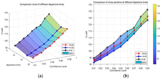
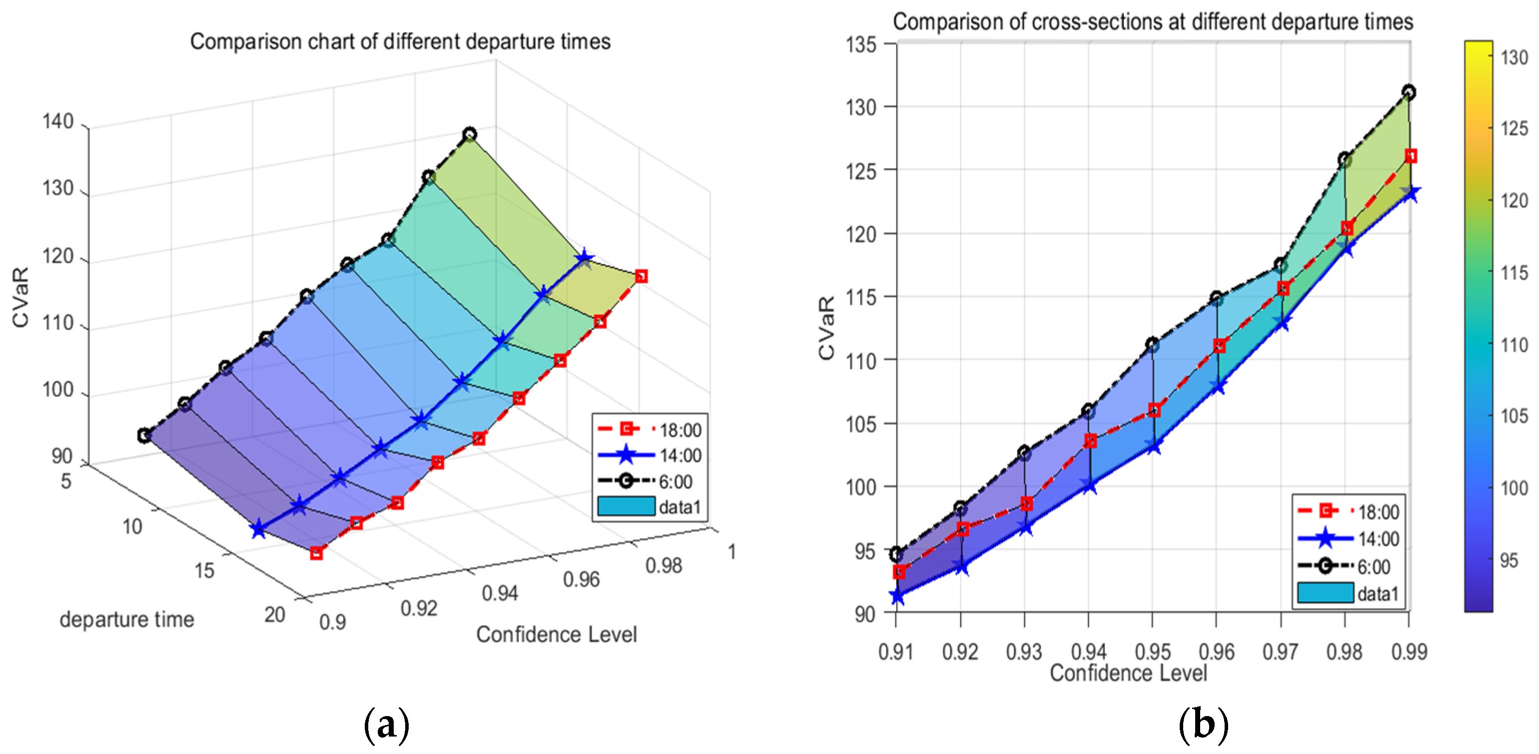
Meanwhile, to better discuss the time-varying characteristics of CVaR, a comparative analysis of CVaR values at departure times of 6:00, 14:00, and 18:00 is conducted, as shown in Figure 8.
Figure 8.
Comparison of optimal CVaR under different departure times. (a) Three-dimensional comparison chart. (b) Two-dimensional comparison chart.
Figure 8 presents an analysis across different confidence levels µ. A higher µ value indicates a stronger aversion of the decision-maker to accidents, while the CVaR value represents the risk consequence under that specific confidence level. Therefore, as the confidence level increases, reflecting a more conservative stance, the resulting risk cost (CVaR) also becomes larger. As shown in Figure 9, the CVaR values for different cargo departure times generally follow a consistent trend, increasing with the confidence level µ. In other words, the optimal CVaR value increases as the decision-maker’s desire to avoid risks in hazardous goods transportation grows. Simultaneously, the rate of increase in the optimal CVaR value strengthens with the decision-maker’s rising risk aversion.
Figure 9.
Multimodal transport network diagram.
At a 0.991 level of confidence, the differences across the three time periods are relatively small. However, when the confidence level exceeds 0.991, the CVaR for the 14:00 departure is lower than that for the 6:00 and 18:00 departures. This indicates that the risk consequence associated with departing at 14:00 is comparatively smaller.
Therefore, selecting different departure times significantly affects the risk-consequence value (CVaR) of hazardous goods transportation. It is essential to select an appropriate departure time accordingly. At the same time, the optimal transport route must be recalculated as the departure time changes. Hence, to effectively manage overall risk in hazardous goods transportation, it is necessary to dynamically select the optimal departure time in conjunction with the target confidence level, compute real-time routes, and fully account for the scheduling constraints of available transport modes.
5.3. Case Study
To validate the model’s practicality, this study uses the route from Chongqing, China (Node 1) to Changchun (Node 16), passing through 14 cities (Nodes 2–15, details in Table 10). Transfers are allowed between each node. The hard time window for delivery is [Tmin, Tmax] = [60 h, 75 h], with a maximum of three transfers allowed. Distances and relevant parameters for different transport modes between nodes are obtained from a map, the China Railway Network, and the China Maritime Safety Administration. Assuming a 30-ton shipment departs from Chongqing at 14:00, transfer times, speed schedules, and costs for different transport modes are calculated using the parameters in Table 4, Table 5 and Table 6. The objective is to identify the transportation scheme with the lowest overall risk within the delivery time constraints.
Table 10.
Number of cities in the multimodal transport network.
With the number of ants in the CSAACO algorithm set to 50, α = 4, and β = 3, the program yields route selection results from Chongqing to Changchun for different confidence levels, as shown in Table 11.
Table 11.
Route selection results from Chongqing to Changchun.
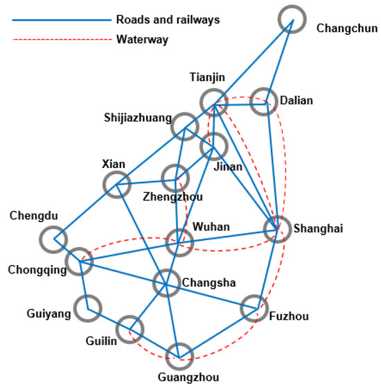
Based on the results above, the route solutions vary substantially across confidence levels. When μ = 0.995, the risk value is 298.52, the total transportation time required is 74.03 h, and the route involves three transfers before arriving in Changchun. The optimal transportation path is shown in Figure 10.
Figure 10.
Diagram of the optimal path selection.
As the confidence level μ increases from 0.991 to 0.999 (i.e., as decision-makers require coverage of more extreme tail risks), the CVaR of the optimal route increases monotonically from 272.58 to 340.22. Notably, at μ = 0.995, a distinct route emerges. Compared with the other two scenarios, this solution introduces an additional transfer (the path includes node “15.3”), resulting in the longest total transportation time (74.03 h), while its CVaR value (298.52) is not the highest. This shows that under a specific risk confidence level, the model actively chooses a “detour” to avoid a segment with extremely high potential consequences (which may be an area with very high population density or extreme environmental sensitivity)—that is, it trades increased transfer frequency and transportation time for a reduction in overall tail risk. This result highlights the complex interplay between the “time window” and the “risk window” and demonstrates that the model does not simply pursue the shortest time but performs sophisticated risk scheduling under multiple constraints. In summary, the case study analysis indicates that it provides managers with a clear, quantitative basis for decision-making to achieve precise trade-offs among “acceptable risk,” “transportation efficiency,” and “operational feasibility.”
6. Conclusions
Based on the Conditional Value-at-Risk (CVaR) theory and considering constraints related to time-varying conditions, schedule restrictions, and time windows, this study formulates a hazardous materials multimodal transport routing optimization model. Ant Colony Optimization (ACO) and CSAACO algorithms are developed to solve the model, selecting the transport route and modes that minimize the total transportation risk throughout the hazardous materials’ multimodal journey. Through case study calculations and comparative analysis, the model’s feasibility and the algorithms’ performance are validated, leading to the following main conclusions:
- At different departure times, the CVaR values vary at the same confidence level, and the selection of hazardous goods intermodal routes also varies with departure time. This indicates that decision-makers need to choose the most appropriate departure time based on their risk preferences and in accordance with the time-varying risk characteristics of hazardous materials transportation.
- Comparative calculations show that the CSAACO algorithm outperforms the standard ACO algorithm in global search when solving this problem. It can effectively escape local optima and explore a larger solution space, thereby obtaining better solutions.
- For future research, environmental hazards should be considered a risk factor. Although the current CVaR model effectively quantifies tail risk, future work could incorporate additional risk dimensions and explore multi-objective collaborative optimization models to balance risk, cost, and timeliness. Furthermore, it is necessary to investigate the hazardous materials route optimization problem using risk-equitable Conditional Value-at-Risk (CVaRE).
- Although the CSAACO algorithm developed in this study delivers strong solution quality, its computational efficiency remains lower than that of emerging deep learning-based approaches. Future research could integrate deep learning techniques and big data analytics to further enhance solution efficiency and scalability. In addition, our study does not consider regulatory restrictions on hazardous materials transportation, such as time-dependent or route-specific prohibitions. Incorporating such regulatory constraints in future work would improve the generality and practical applicability of both the proposed model and the solution algorithm.
From a managerial and policy perspective, the proposed CVaR-based multimodal routing framework offers a practical decision-support tool for balancing transportation safety and operational efficiency under uncertainty. For logistics managers, the results indicate that both risk aversion and departure time are decisive in route and mode selection, underscoring the need to dynamically adjust transportation plans to reflect managers’ risk preferences and the time-varying characteristics of population exposure, traffic conditions, and schedule constraints. By explicitly controlling tail risk, the model enables decision-makers to avoid low-probability but catastrophic events, thereby enhancing the robustness and safety of hazardous materials transportation systems. For policymakers and regulatory authorities, the model provides a quantitative basis for designing risk-oriented transportation regulations, such as differentiated routing guidelines, time-dependent transport restrictions, and safety standards that reflect extreme-risk considerations. Moreover, incorporating schedule constraints and transshipment limitations makes the proposed approach particularly suitable for real-world multimodal networks, supporting the coordinated management of rail and waterway operations.
Author Contributions
Conceptualization, S.L.; Methodology, S.L. and Y.P.; Software, Y.P. and Y.L. (Yi Liu); Validation, Y.L. (Yazhi Lin), D.Z.Y., Y.P., Y.L. (Yi Liu) and X.M.; Formal analysis, S.L., J.L. and Y.L. (Yazhi Lin); Investigation, S.L., J.L. and Y.L. (Yazhi Lin); Data curation, J.L., Y.L. (Yi Liu) and X.M.; Writing—original draft, J.L. and Y.L. (Yazhi Lin); Writing—review and editing, D.Z.Y.; Visualization, D.Z.Y. and X.M.; Supervision, D.Z.Y.; Project administration, S.L.; Funding acquisition, S.L. All authors have read and agreed to the published version of the manuscript.
Funding
This research was funded by the Team Building Project for Graduate Tutors in Chongqing (Grant No. JDDSTD2022004) and was supported by the Project of Science and Technology Research Program of the Chongqing Education Commission of China (No. KJQN202400750).
Data Availability Statement
The original contributions presented in this study are included in the article. Further inquiries can be directed to the corresponding author.
Conflicts of Interest
The authors declare no conflicts of interest.
References
- Wang, Z.X.; Huang, Y.H.; Ren, Z.; Luo, Z.J. Identification, assessment and compensation of ecological and environmental damage caused by hazardous material transportation accidents in China. Saf. Environ. Eng. 2022, 29, 248–254. [Google Scholar] [CrossRef]
- Karimi, A.; Khajevandi, A.A.; Ebrahimi, M.; Sarsangi, V. Analysis and prioritization of management factors influencing the risk of hazardous materials road transport accidents using the fuzzy analytic hierarchy process. Arch. Trauma. Res. 2025, 14, 17–25. [Google Scholar] [CrossRef]
- Mohri, S.S.; Mohammadi, M.; Gendreau, M.; Pirayesh, A.; Ghasemaghaei, A.; Salehi, V. Hazardous material transportation problems: A comprehensive overview of models and solution approaches. Eur. J. Oper. Res. 2022, 302, 1–38. [Google Scholar] [CrossRef] [Scilit]
- Du, J.; Li, X.; Yu, L.; Dan, R.; Zhou, J. Multi-depot vehicle routing problem for hazardous materials transportation: A fuzzy bilevel programming. Inf. Sci. 2017, 399, 201–218. [Google Scholar] [CrossRef] [Scilit]
- Ma, C.; Mao, B.; Xu, Q.; Hua, G.; Zhang, S.; Zhang, T. Multi-Depot vehicle routing optimization considering energy consumption for hazardous materials transportation. Sustainability 2018, 10, 3519. [Google Scholar] [CrossRef] [Scilit]
- Ma, C.; Hao, W.; Pan, F.; Xiang, W. Road screening and distribution route multi-objective robust optimization for hazardous materials based on neural network and genetic algorithm. PloSone 2018, 13, 0198931. [Google Scholar] [CrossRef] [Scilit]
- Zhang, L.; Feng, X.; Yang, Y.; Ding, C. Routing for hazardous materials transportation in urban areas. Symmetry 2019, 11, 1091. [Google Scholar] [CrossRef] [Scilit]
- Wang, Z.Z.; Wu, Z.H.; Liu, W.J. Multi-Depot Half-Open hazardous materials transportation routing considering optimization customer relationships. J. Tongji Univ. 2025, 53, 741–748. [Google Scholar] [CrossRef]
- Shi, J.Y.; Huang, H.Y. Optimization of vehicle routing for hazardous material transportation in time-varying risk environments. J. Saf. Environ. 2024, 24, 4416–4423. [Google Scholar] [CrossRef]
- Ma, T.M.; Huang, C.Y.; Chen, X.F. Heterogeneous vehicle routing problem of hazardous materials transportation considering carbon emissions. China Saf. Sci. J. 2024, 34, 193–199. [Google Scholar] [CrossRef]
- Chai, H.; He, R.C.; Han, W.; Jia, X.Y.; Dai, C.J. Two-stage optimization of vehicle routing problem for hazardous materials with time windows. China Saf. Sci. J. 2023, 33, 160–166. [Google Scholar] [CrossRef]
- Zhang, K.Y.; Wen, H.J.; Chen, Y.P.; Meng, H.Y.; Ju, Y.T. Vehicle transport path optimization method of hazardous chemicals based on digital twin technology. Sci. Technol. Eng. 2023, 23, 14676–14681. [Google Scholar] [CrossRef]
- Wang, X.Q.; Dai, C.J.; Li, J.; Wu, R.Y. Optimization of green distribution routes for hazardous materials under uncertain transportation risk. Comput. Eng. Appl. 2023, 59, 323–332. [Google Scholar] [CrossRef]
- Wang, J.; Liu, F.; Xu, Y.; Zhao, C.Z. Study on optimization of dangerous goods transportation route considering risk impedance. J. Chang. Univ. Sci. Technol. Nat. Sci. 2023, 59, 163–170. [Google Scholar] [CrossRef]
- Kuang, Y.J.; Zhao, J.H. Location and routing of dangerous goods storage and transportation under continuous time-varying risks. China Saf. Sci. J. 2022, 32, 185–191. [Google Scholar] [CrossRef]
- Zhang, W.; Chen, X.; Jia, H.X.; Zhang, H.X. Research on the optimal model of dangerous goods transportation routes. Highw. Automot. Appl. 2025, 41, 44–50. [Google Scholar] [CrossRef]
- Wang, Q.; Yang, X.F.; Li, N.; Li, P.; Wang, X.F. Route optimization of hazardous materials transportation vehicles in uncertain environment. Comput. Eng. Appl. 2022, 58, 309–316. [Google Scholar] [CrossRef]
- Liang, X.; Li, X.; Zhang, C. A fuzzy programming method for modeling demand uncertainty in the capacitated road–rail multimodal routing problem with time windows. Symmetry 2019, 11, 91. [Google Scholar] [CrossRef] [Scilit]
- Jia, X.Y.; He, R.C.; Chai, H.; Zhang, C.M.; Zhang, T.; Huang, Z.P.; Li, H.T.; Fang, Y. Path model for hazmat rail-road intermodal transportation in spatiotemporal service network. J. China Railw. Soc. 2023, 45, 20–28. [Google Scholar] [CrossRef]
- Li, X.; Lei, M.M.; Liu, G.X. Path optimization for road-rail intermodal transport of dangerous goods considering regional risk equity. Railw. Transp. Econ. 2024, 46, 140–149. [Google Scholar] [CrossRef]
- Fang, Y.; Jia, X.Y. Route Hazmat route optimization by road-rail intermodal transport in the silk road economic zone. Sci. Technol. Eng. 2023, 23, 6614–6622. [Google Scholar] [CrossRef]
- Li, P.; Zhu, Z.L.; Chang, D.F. Study on path optimization for multimodal transport of dangerous goods based on multi-period. J. Saf. Sci. Technol. 2019, 15, 151–156. [Google Scholar] [CrossRef]
- He, Z.G.; Guo, J.N.; Xu, J.X. Security risk assessment for the risk cargos transportation in the multimodal transfer based on the hesitative intuitionistic fuzzy set-TOPSIS. J. Saf. Environ. 2020, 20, 19–24. [Google Scholar] [CrossRef]
- Kang, Y.; Batta, R.; Kwon, C. Value-at-Risk model for hazardous material transportation. Ann. Oper. Res. 2013, 222, 361–387. [Google Scholar] [CrossRef] [Scilit]
- Kang, Y.; Batta, R.; Kwon, C. Generalized route planning model for hazardous material transportation with VaR and equity considerations. Comput. Oper. Res. 2014, 43, 237–247. [Google Scholar] [CrossRef] [Scilit]
- Wang, Z.Z.; Zhao, L.Y.; Cao, N.B.; Yu, M.M.; Chen, M.T. The route choice of hazardous material transportation with value-at-risk model using chance measure in uncertain environments. Adv. Mech. Eng. 2018, 10, 1687814017753801. [Google Scholar] [CrossRef] [Scilit]
- Wei, F.L.; Liu, P.; Li, Z.B.; Sun, F.; Guo, Y.Q.; Zhao, L.Y.A. An optimal routing method of hazardous materials transportation based on VaR. J. Transp. Inf. Saf. 2020, 38, 17–23. [Google Scholar] [CrossRef]
- Toumazis, I.; Kwon, C. Routing hazardous materials on time-dependent networks using conditional value-at-risk. Transp. Res. Part C 2013, 37, 73–92. [Google Scholar] [CrossRef] [Scilit]
- Faghih-Roohi, S.; Ong, Y.-S.; Asian, S.; Zhang, A.N. Dynamic conditional value-at-risk model for routing and scheduling of hazardous material transportation networks. Ann. Oper. Res. 2016, 247, 715–734. [Google Scholar] [CrossRef] [Scilit]
- He, Z.G.; Zhang, C.; Fang, J. Variable path-ways selection for the transportation of hazardous goods based on the conditional value. J. Saf. Environ. 2018, 18, 428–433. [Google Scholar] [CrossRef]
- Cao, H.; Fan, T.J.; Liu, L.P. Routing the road and railway intermodal transportation of hazmat based on CVaR. Oper. Res. Manag. Sci. 2017, 26, 41–48. [Google Scholar]
- Hosseini, S.D.; Verma, M. Equitable routing of rail hazardous materials shipments using CvaR methodology. Comput. Oper. Res. 2021, 129, 105222. [Google Scholar] [CrossRef] [Scilit]
- Liu, L.; Sun, S.; Li, S. Route optimization of hazardous material railway transportation based on Conditional Value-at-Risk considering risk equity. Mathematics 2025, 13, 803. [Google Scholar] [CrossRef] [Scilit]
- Duan, Y.L.; Zhao, S.Y.; Roy, N.; Zhang, B. Understanding the effect of buildings and environmental factors in hazardous material transportation using multi-objective Conditional Value at Risk (CVaR). J. Loss Prev. Process Ind. 2025, 97, 105678. [Google Scholar] [CrossRef] [Scilit]
- Erkute, V. Modeling of transport risk for hazardous materials. Oper. Res. 1998, 46, 625–642. [Google Scholar] [CrossRef] [Scilit]
- Xi, J.P.; Zhang, J.R.; Dong, H.-X.; Wang, N. Vehicle routing optimization of intra-city freight considering demand change and time-varying road network. J. Chang. Univ. Nat. Sci. Ed. 2023, 43, 137–150. [Google Scholar] [CrossRef]
- Ahmed, Z.H.; Hameed, A.S.; Mutar, M.L.; Haron, H. An enhanced ant colony system algorithm based on subpaths for solving the capacitated vehicle routing problem. Symmetry 2023, 15, 2020. [Google Scholar] [CrossRef] [Scilit]
- Solomon, M. Algorithms for the vehicle routing and scheduling problems with time window constraints. Oper. Res. 1997, 35, 254–265. [Google Scholar] [CrossRef] [Scilit]
- Harwood, D.W.; Viner, J.G.; Russell, E.R. Procedure for developing truck accidents and release rates for hazmat routing. J. Transp. Eng. 1993, 119, 189–199. [Google Scholar] [CrossRef] [Scilit]





Disclaimer/Publisher’s Note: The statements, opinions and data contained in all publications are solely those of the individual author(s) and contributor(s) and not of MDPI and/or the editor(s). MDPI and/or the editor(s) disclaim responsibility for any injury to people or property resulting from any ideas, methods, instructions or products referred to in the content. |
© 2026 by the authors. Licensee MDPI, Basel, Switzerland. This article is an open access article distributed under the terms and conditions of the Creative Commons Attribution (CC BY) license.