


Abstract
Soil visible–near-infrared (Vis-NIR) spectroscopy enables rapid, high-throughput estimation of soil physicochemical properties, but complex deep learning models can increase computational cost and reproducibility burden. This study developed a lightweight full-spectrum embedding multilayer perceptron (LSE-MLP) for simultaneous prediction of soil pH, organic carbon (OC), and total nitrogen (N). LSE-MLP maps 4200-dimensional spectra into a compact, learnable representation and uses residual MLP modules for subsequent nonlinear regression. Using the LUCAS2009 dataset, LSE-MLP was compared with PLSR, SVR-RBF, 1D-CNN, ResNet-1D, and Transformer-1D under a POINT_ID-grouped cross-validation framework. Model performance was assessed using internal split sensitivity analysis, ablation experiments, multi-random-seed analysis, and an independent blind test set. On this test set, LSE-MLP achieved R2 values of 0.9437, 0.9519, and 0.9363 for pH, OC, and N, respectively. Its computational efficiency was primarily reflected in low floating-point operations (FLOPs) and fast batch CPU inference, rather than the smallest parameter count or model storage footprint. Supplementary experiments indicated that band compression reduced input dimensionality with limited performance loss, whereas direct transfer of frozen LUCAS-trained models to KSSL and AUT showed substantial performance degradation associated with spectral and target-distribution differences. Overall, LSE-MLP provides a practical and computationally efficient option for soil property prediction using Vis-NIR spectroscopy under the evaluated conditions, while reliable cross-dataset transfer requires further investigation.
1. Introduction
Soil pH, organic carbon (OC), and total nitrogen (N) are key indicators in soil quality assessment, agricultural management, and research on ecological functions. Conventional laboratory analyses can provide reliable measurements, but sample collection, preparation, and chemical analysis are time-consuming and costly, limiting data acquisition efficiency in large-scale surveys and high-frequency monitoring. To improve assessment efficiency, previous studies have combined sensor measurements with machine learning for the rapid estimation of soil properties [1].
Visible–near-infrared (Vis-NIR) spectroscopy is commonly used in research on rapid soil property prediction [2]. Organic matter, moisture, mineral composition, and particle characteristics influence light absorption and scattering in soil, producing spectral information related to soil physicochemical properties [3]. Compared with conventional chemical analysis, Vis-NIR measurements are non-destructive and rapid, require less sample preparation, and allow multiple properties to be estimated from a single spectrum [4]. These advantages make the technique suitable for analyzing large numbers of samples, but predictive performance still depends on the model’s ability to identify useful information in the spectra. Scattering effects and measurement noise can interfere with spectral signals, while sample heterogeneity and nonlinear relationships between spectra and soil properties complicate modeling. Therefore, extracting stable and useful information for prediction from high-dimensional continuous spectra remains a key challenge in soil spectral modeling [5].
In soil Vis-NIR modeling, partial least squares regression (PLSR) is commonly used as a linear baseline for high-dimensional spectral data, particularly when sample sizes are relatively limited. Support vector regression (SVR), by contrast, uses kernel functions to characterize nonlinear relationships between spectra and soil properties. Among neural network models, the multilayer perceptron (MLP) learns nonlinear mappings between spectral variables and target properties through fully connected layers and has been applied to predict multiple soil properties using LUCAS data [6]. One-dimensional convolutional neural networks (1D-CNNs) use local convolutions to extract features from adjacent wavelengths [7]. Hybrid convolutional-recurrent networks, encoder–decoder architectures, and Transformer-based models have also been applied to soil spectral modeling [8,9,10,11]. Previous studies have shown that deep models can learn soil property-related representations from spectral data [12,13] and achieve high predictive accuracy under certain datasets and validation settings [14].
However, increasing model complexity does not necessarily yield predictive gains commensurate with the associated computational cost. Discussions of green artificial intelligence have emphasized that model evaluation should consider not only predictive accuracy but also resource consumption, reproducibility, and deployment cost [15]. For large-scale soil spectral data, complex deep models typically incur greater computational overhead [16] and impose greater demands on architecture design and hyperparameter tuning [17]. Recent studies in soil spectroscopy have also begun to evaluate lightweight models in terms of parameter count, computational cost, and inference speed [18]. Meanwhile, model performance estimates can also be affected by the data-splitting strategy [19]. Because soil samples may include repeated sampling points, spatial clustering, and regional similarity, sample-level random splitting may assign highly similar samples to both the training and test sets, resulting in overly optimistic performance estimates. Therefore, the evaluation of soil spectral prediction models should consider not only conventional accuracy metrics but also the risk of sampling-point-level information leakage, data-splitting strategies, result stability, and computational efficiency [20].
To address these issues, this study developed a lightweight full-spectrum embedding multilayer perceptron (LSE-MLP) for simultaneous prediction of soil pH, organic carbon (OC), and total nitrogen (N). The architecture combines a learnable linear projection of the complete 4200-dimensional Vis-NIR spectrum with residual MLP blocks operating in a compact latent space. Its design is motivated by the distinction between retaining access to all spectral variables and performing computationally efficient nonlinear regression on a lower-dimensional representation. Unlike approaches that primarily extract local spectral features through convolution or model feature interactions through self-attention, LSE-MLP uses a direct full-spectrum embedding followed by compact nonlinear feature refinement. The individual architectural components are established techniques; the contribution investigated here is their task-oriented integration and systematic evaluation for multi-property soil spectral regression. Using LUCAS2009, we evaluated this design against PLSR, SVR-RBF, 1D-CNN, ResNet-1D, and Transformer-1D through POINT_ID-grouped validation, an independent blind test set, ablation and stability analyses, and computational efficiency measurements. Additional experiments examined band compression and cross-dataset applicability.
The main contributions of this study are fourfold. First, we designed a full-spectrum multi-property regression framework that integrates a learnable linear spectral embedding with residual MLP blocks. The architecture allows all input wavelengths to contribute to a compact representation before subsequent nonlinear processing, without requiring explicit wavelength preselection. Second, we examined the contribution of this design through comparisons with five conventional and deep learning baselines, together with embedding and residual-connection ablations and hyperparameter sensitivity analyses. Third, we evaluated predictive accuracy, stability, and computational efficiency under POINT_ID-grouped validation and an independent blind test set, providing an empirical assessment of the accuracy–efficiency trade-off. Fourth, we investigated band compression and external-dataset applicability to assess the potential for reducing input dimensionality and to identify limitations associated with cross-dataset transfer.
2. Materials and Methods
2.1. Dataset and Spectral Preprocessing
This study used the publicly available LUCAS2009 topsoil Vis-NIR spectral dataset for soil property prediction. LUCAS Soil is an open data resource widely used for soil monitoring and property mapping across Europe [21]. After screening, 19,036 valid samples were retained, each containing 4200 spectral variables covering approximately 400–2499 nm. The prediction targets were soil pH, OC, and N. Descriptive statistics for each target property are provided in Table S1. Information on data access is provided in the Data Availability Statement at the end of the manuscript.
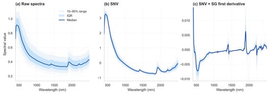
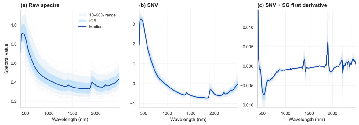
Soil Vis-NIR spectra are affected by particle composition, scattering effects, baseline variations, and measurement noise. To assess the effects of preprocessing on predictive performance, this study evaluated three spectral input forms: raw spectra, standard normal variate (SNV) transformation, and SNV combined with the Savitzky–Golay first derivative (SNV + SG-1D). SNV was used to reduce differences in scale between samples and mitigate scattering effects. Savitzky–Golay first derivative processing highlighted local spectral variations through smoothing and differentiation. SNV + SG-1D was used as the default preprocessing method in the main experiments. The spectral profiles of the three input forms are shown in Figure 1.
Figure 1.
Soil Vis-NIR spectral profiles obtained using different preprocessing methods. (a) Raw spectra; (b) spectra after standard normal variate (SNV) transformation; and (c) spectra after SNV transformation combined with the Savitzky–Golay first derivative (SNV + SG-1D). For each preprocessing method, 500 samples were randomly selected for visualization. The dark solid line represents the median spectrum, whereas the inner and outer shaded regions denote the 25th–75th and 10th–90th percentile ranges, respectively. The light curves represent a randomly selected subset of individual spectra.
2.2. Data Partitioning and Validation Protocol
The screened 19,036 valid samples corresponded to 19,010 unique POINT_IDs, indicating that a small number of records shared the same sampling-point identifier. To reduce the risk of information leakage caused by assigning samples from the same sampling point to different subsets, a fixed data partition was generated before the experiments using POINT_ID as the grouping unit. All samples were split at an approximate ratio of 80:20 into a development set (15,230 samples) and an independent blind test set (3806 samples), with the constraint that the same POINT_ID could not appear in both sets. The development set was used for model training, hyperparameter selection, cross-validation, ablation experiments, parameter sensitivity analysis, and supplementary experiments. The independent blind test set was used only once for final evaluation after the final model configuration and supplementary experimental strategies had been determined.
Within the development set, POINT_ID-grouped five-fold cross-validation was used as the main protocol for model selection and performance comparison. Samples in the development set were divided into five non-overlapping folds according to POINT_ID. In each run, four folds were used for model training, and the remaining fold was used for validation. The mean and standard deviation of the evaluation metrics were then reported.
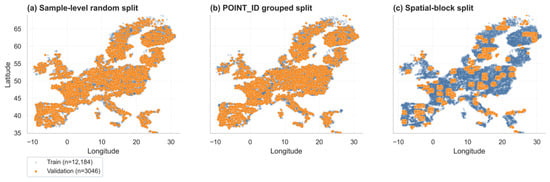
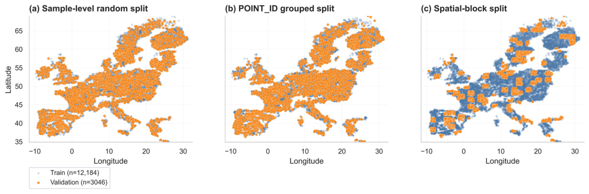
To examine the influence of data partitioning on performance estimation and relative model performance, three additional internal validation protocols were used: sample-level random split, POINT_ID-grouped split, and spatial-block split. For the spatial-block split, 100 km spatial groups were constructed based on sample longitude and latitude. Under all three protocols, training and validation sets were generated within the development set at an approximate ratio of 80:20. Because the validation samples were not identical across the three protocols, this comparison was used only to evaluate the sensitivity of the results to the partitioning strategy, rather than to assume a predefined difficulty order among the protocols. The spatial distributions of the training and validation samples under the three internal validation protocols are shown in Figure 2.
Figure 2.
Spatial distributions of training and validation samples under three internal validation protocols within the development set. (a) Sample-level random split; (b) POINT_ID-grouped split; and (c) spatial-block split. Semi-transparent blue points represent training samples, whereas orange points represent validation samples. The corresponding sample sizes are provided in each legend. Each protocol generated its own training and validation subsets. The displayed longitude and latitude ranges were determined using the 1st–99th percentiles of all sample coordinates to reduce the influence of extreme coordinate values on visualization.
To evaluate training randomness, ResNet-1D, Transformer-1D, and LSE-MLP were repeatedly trained using random seeds of 42, 2023, 2024, 2025, and 3407. The means and standard deviations of the average R2 and average ratio of performance to deviation (RPD) were reported. All methodological decisions, including spectral preprocessing, model architecture, hyperparameter selection, and band-compression strategy, were based exclusively on the development set and its internal validation results. The independent blind test set was reserved for final evaluation after these decisions had been fixed, and its results were not used to modify the selected configurations or compression strategy.
2.3. Comparative Models and Hyperparameter Selection
To evaluate the predictive performance of LSE-MLP, this study selected PLSR, SVR-RBF, 1D-CNN, ResNet-1D, and Transformer-1D as comparative models. PLSR was used as a traditional chemometric linear baseline, and SVR-RBF was used as a nonlinear kernel-based baseline [22,23]. The 1D-CNN, ResNet-1D, and Transformer-1D models represented local convolutional, residual convolutional, and self-attention-based approaches to spectral modeling, respectively. All models were evaluated using consistent data partitions, spectral preprocessing procedures, and performance metrics. The neural models also followed the same target-standardization, optimization, and early-stopping procedures. However, the comparison did not impose identical hyperparameter search budgets or training sample sizes across all model families.
For each model, a finite set of candidate configurations was evaluated using POINT_ID-grouped five-fold cross-validation within the development set. During hyperparameter selection, neural network training was limited to a maximum of 120 epochs, with an early-stopping patience of 15 epochs. Final configurations were selected primarily according to mean validation R2, with mean RPD and RMSE considered as secondary criteria. The candidate sets differed in size and parameter coverage, reflecting the distinct architectures and computational requirements of the models. In particular, SVR-RBF was trained using at most 4000 samples per fold for computational feasibility, whereas this subsampling restriction was not applied to the other models. The evaluated candidates and selected configurations are documented in Table S2, and the sensitivity of LSE-MLP to its architectural hyperparameters is reported in Table S3. The independent blind test set was excluded from hyperparameter selection. Consequently, the comparisons characterize performance under the implemented training and tuning protocols rather than performance under equal optimization budgets or exhaustive model-specific tuning.
2.4. LSE-MLP Model Architecture
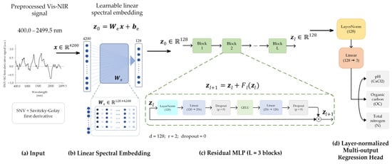
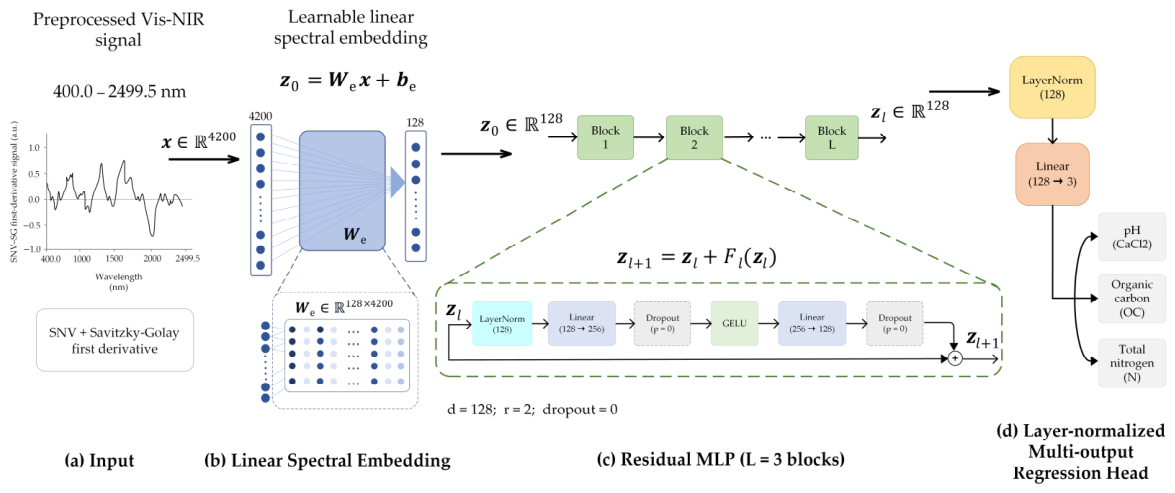
The lightweight full-spectrum embedding multilayer perceptron (LSE-MLP) developed in this study was designed for soil Vis-NIR spectral sensing tasks. Its overall architecture is shown in Figure 3.
Figure 3.
Schematic architecture of the LSE-MLP model. (a) Preprocessed full-spectrum Vis-NIR input. (b) Learnable linear spectral embedding. (c) Residual MLP blocks for nonlinear feature refinement. (d) A layer-normalized multi-output linear regression head for simultaneous prediction of pH (CaCl2), organic carbon (OC), and total nitrogen (N).
The model consisted of a linear spectral embedding (LSE) layer, residual MLP modules, and a multi-property regression output head for the joint prediction of soil pH, OC, and N. The architectural rationale is to decouple full-spectrum feature projection from subsequent nonlinear regression. Specifically, each latent feature produced by the learnable embedding can depend on the entire input spectrum, while the residual MLP blocks operate on the lower-dimensional representation rather than directly processing the original 4200 spectral variables. This arrangement provides an alternative to architectures that rely primarily on local convolutional feature extraction or self-attention-based interactions. The embedding layer and residual connections are not novel operations individually; their role in LSE-MLP is to provide a compact, task-oriented architecture for joint soil-property prediction. The effectiveness of these design choices was examined through component ablations and accuracy-efficiency comparisons. For each soil sample, the model input was the preprocessed Vis-NIR spectral vector: , where p = 4200 denotes the number of spectral features. A learnable LSE layer was used to map the full-spectrum input into a d-dimensional latent space, reducing input dimensionality while retaining full-spectrum information. This process was expressed as:
where and are the weight matrix and bias term of the embedding layer, respectively; is the low-dimensional spectral embedding representation; and d is the embedding dimension. Unlike fixed average pooling, the learnable LSE layer can form a full-spectrum linear representation related to the prediction task during supervised training. The contribution of this design was evaluated through an average-pooling embedding ablation experiment.
After the low-dimensional full-spectrum representation was obtained by the LSE layer, residual MLP modules were used to further model nonlinear relationships in the latent features. The l-th residual MLP module was expressed as:
where denotes an MLP transformation composed of fully connected layers, nonlinear activation functions, dropout, and related operations. The residual connection was used to preserve the input representation while adding nonlinear transformation information.
The embedding dimension and the number of residual MLP blocks were determined by considering the representational capacity and computational complexity of the model, followed by validation-based configuration selection. The embedding dimension controls the width of the latent representation and, consequently, the computational cost of the subsequent nonlinear layers. A very small latent dimension may restrict the information available for regression, whereas increasing the dimension introduces additional parameters without necessarily improving predictive performance. Similarly, the number of residual blocks determines the depth of nonlinear feature refinement. A shallow architecture may provide insufficient flexibility to capture complex spectral–property relationships, while additional blocks increase model complexity and may offer diminishing predictive benefits. These considerations motivated the evaluation of compact embedding dimensions and relatively shallow residual architectures. The final configuration, comprising an embedding dimension of 128 and three residual MLP blocks, was selected from the evaluated candidates using POINT_ID-grouped cross-validation within the development set. The corresponding hyperparameter sensitivity results are reported in Table S3.
After several residual MLP modules, the final latent representation was passed to a linear regression output head to generate predictions for the three soil properties:
where , corresponding to pH, OC, and N. This study adopted a multi-output regression form with shared spectral representations. Specifically, the three properties shared the LSE layer and residual MLP representation, and the same regression head produced the multi-property prediction outputs. The standardization and inverse standardization of target variables are described in Section 2.5.
Deep learning models were trained using the mean absolute error calculated on standardized targets. Let and denote the standardized observed and predicted values of the t-th property for the i-th sample, respectively, and let denote the number of predicted properties. The training loss was defined as:
This loss corresponds to L1Loss in PyTorch and jointly optimizes the absolute errors of the three standardized targets, namely pH, OC, and N. During model evaluation, predicted values were inverse-standardized to the original scale before all evaluation metrics were calculated.
Compared with 1D-CNN, ResNet-1D, and Transformer-1D, LSE-MLP does not use local convolutional kernels or self-attention computation among spectral patches. Instead, it first obtains a low-dimensional full-spectrum representation through learnable LSE and then uses residual MLP modules for nonlinear mapping. The performance of this architecture for pH, OC, and N prediction was evaluated through model comparison, ablation experiments, and efficiency analysis.
2.5. Model Training, Evaluation Metrics, and Ablation Design
All deep learning models were trained using a unified training procedure, including mini-batch optimization, early stopping, and saving of the model weights with the best validation performance. To reduce the influence of differences in units and numerical ranges among pH, OC, and N, the target variables were standardized during training and the predicted values were inverse-standardized to the original scale during evaluation. Because differences in spectral preprocessing, modeling algorithms, and evaluation procedures can affect soil property prediction using Vis-NIR spectroscopy [24], both traditional machine learning models and deep learning models were trained and compared using the same data partitions, preprocessed inputs, and evaluation metrics. In the band compression experiment, full-spectrum LSE-MLP and band-compressed LSE-MLP used the same final training protocol to ensure a consistent comparison.
Model predictive performance was evaluated using the coefficient of determination (R2), root mean squared error (RMSE), mean absolute error (MAE), and ratio of performance to deviation (RPD). These metrics were calculated as follows:
where and denote the observed and predicted values of the i-th sample, respectively; is the mean of the observed values; and is the standard deviation of the observed values. Because pH, OC, and N differ in units and numerical ranges, the evaluation metrics for each property were reported separately in the main results tables. The average R2 and average RPD were used only for overall performance visualization and accuracy–efficiency trade-off analysis.
Ablation experiments were conducted to analyze the contribution of key LSE-MLP components to predictive performance. The complete LSE-MLP consisted of SNV + SG-1D spectral preprocessing, a learnable linear spectral embedding (LSE) layer, and residual MLP modules. The ablation settings included replacing the main preprocessing method with raw spectra or SNV transformation only, removing residual connections, and replacing the learnable LSE layer with average-pooling embedding. In addition, the effects of embedding dimension, network depth, MLP ratio, and dropout on model performance were examined.
All neural network models were trained using the AdamW optimizer with a constant learning rate of 3 × 10⁻⁴ and a batch size of 128. No learning-rate scheduler was employed. During the final POINT_ID-grouped five-fold cross-validation, training was conducted for a maximum of 200 epochs, with early stopping based on the validation loss calculated as the arithmetic mean of batch-wise mean absolute errors on standardized targets. Training was terminated when the monitored loss failed to decrease for 20 consecutive epochs. No positive minimum-improvement threshold was imposed; any strict decrease in the monitored loss was considered an improvement. For each fold, the checkpoint corresponding to the lowest monitored validation loss was retained for evaluation.
The experiments were conducted on a workstation running Windows 11 Pro (build 26200), equipped with an Intel Core i5-12600KF CPU (Intel Corporation, Santa Clara, CA, USA) and an NVIDIA GeForce RTX 5060 GPU (NVIDIA Corporation, Santa Clara, CA, USA). The recorded training environment comprised Python 3.11.14 and PyTorch 2.10.0.dev20251022+cu128, with PyTorch built against CUDA 12.8.
CPU inference latency was measured on an Intel Core i5-12600KF CPU using preprocessed and standardized spectra from the independent blind test set. For each model and inference setting, 10 warm-up iterations were performed before timing. Single-sample latency was measured over 200 repeated inference calls using the first blind-test spectrum, whereas batch-128 latency was measured over 50 repeated calls using the first 128 blind-test spectra. Average latency was calculated by dividing the total elapsed time by the number of timed repetitions; for batch-128 inference, the resulting batch latency was further divided by 128. The measurements excluded disk I/O, model initialization and weight loading, spectral preprocessing, standardization, input tensor construction, and inverse transformation of the predicted targets. The benchmarking script did not explicitly fix the number of CPU threads, and the original thread configuration and software versions were not recorded. Therefore, the reported latency values should be interpreted as measurements obtained under the original benchmarking conditions rather than as hardware-independent estimates.
To quantify uncertainty in pairwise model comparisons, a paired POINT_ID-cluster bootstrap analysis was performed using the saved out-of-fold predictions from the development-set five-fold cross-validation. A total of 2000 bootstrap resamples (seed = 42) were generated by resampling POINT_ID groups with replacement, applying the same sampled groups to LSE-MLP and each baseline. Differences in R2, RMSE, and MAE were calculated for each soil property, and pointwise 95% confidence intervals were obtained from the bootstrap percentile distribution. The analysis was conditional on the saved predictions and fixed cross-validation partition; no adjustment for multiple comparisons was applied. The independent blind test set was not involved.
2.6. Computational Efficiency and Spectral Importance Analysis
In addition to predictive accuracy, this study evaluated the computational efficiency of each model using the number of parameters, model file size, approximate floating-point operations (FLOPs) per sample, and CPU inference latency. Inference latency was measured using real spectral inputs from the independent blind test set under the same CPU environment. Because the number of parameters alone may not fully represent computational efficiency, FLOPs, inference latency, model file size, and predictive performance were jointly considered to analyze the computational characteristics of different models.
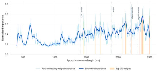
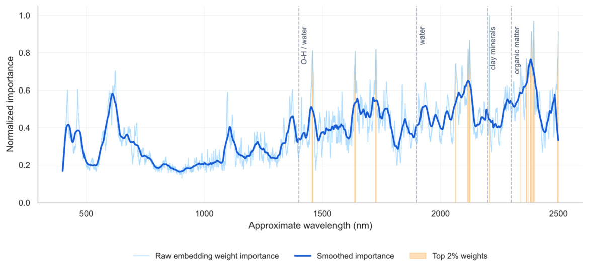
To examine the relative sensitivity of LSE-MLP to different wavelength positions, wavelength importance was calculated based on the weights of the linear spectral embedding (LSE) layer. Let the embedding-layer weight matrix be , and the importance of the j-th wavelength position was defined as:
The resulting values were then normalized to the range of 0–1 and smoothed to visualize the relative sensitivity regions of the model across the full spectrum. This analysis was used only as an auxiliary weight-level interpretation and was not used to directly infer the mechanistic meaning of specific soil spectral bands.
2.7. Supplementary Band Compression Experiment
Previous studies on soil Vis-NIR spectroscopy have shown that spectral variable selection or the use of spectral subsets may affect soil property prediction performance [25]. To evaluate the accuracy–efficiency performance of LSE-MLP under reduced input bands, this study conducted a continuous band-group compression experiment. Without changing the main architecture of LSE-MLP, the 4200 spectral features were divided at the input level into 210 continuous band groups, with each group containing 20 adjacent features. Band-group ranking was then learned within the development set.
The band selection process was restricted to the development set. For each outer fold, internal splitting, gating learning, band-group selection, model retraining, and outer-fold validation were performed independently, and the outer validation fold was not used for learning the gating weights. This study compared shared ranking, property-aware balanced, random continuous band groups, and evenly spaced continuous band groups as selection strategies [26]. The final compression strategy was determined based on the POINT_ID-grouped five-fold cross-validation results, and the final candidate strategy was further evaluated for stability through multi-random-seed experiments.
After the strategy was fixed, the final band set was learned using the complete development set. Full-spectrum LSE-MLP and band-compressed LSE-MLP were then trained separately using the same final training protocol and evaluated once on the independent blind test set.
2.8. Supplementary Validation on External Datasets
To evaluate the applicability of LSE-MLP across different soil spectral data sources, this study introduced two external soil spectral datasets: the Kellogg Soil Survey Laboratory (KSSL) dataset and the Austrian Near-Infrared (NIR) Soil Spectral Library (AUT). Because cross-instrument, cross-regional, and cross-soil-type spectral modeling may be affected by differences in calibration consistency, data harmonization, and property definitions [27,28,29], these supplementary experiments included data auditing, data harmonization, internal validation within each external dataset, and direct transfer tests from LUCAS to the external datasets. The KSSL and AUT results were used only for supplementary evaluation and were not used for primary model selection or parameter tuning.
The data audit focused on the matching relationship between spectral tables and property tables, wavelength ranges, missing values, target property fields, units, and measurement methods. A property was included in subsequent modeling or transfer evaluation only when its definition, unit, and measurement system could be reasonably aligned.
For internal validation within the external datasets, grouped five-fold cross-validation was conducted separately within KSSL and AUT. The predictive performance of PLSR, SVR-RBF, 1D-CNN, ResNet-1D, Transformer-1D, and LSE-MLP was compared. Each model used the final configuration from the main experiment, with only the input and output dimensions adjusted according to the number of input bands and available target properties in the external dataset. Within the same dataset, all models used consistent samples, preprocessing procedures, and fold partitions.
In the direct transfer experiment, models were trained using the LUCAS development set, and their parameters were then frozen. KSSL and AUT were evaluated once without using external data labels for parameter tuning, band selection, or model correction. For AUT, the common wavelength range shared with LUCAS was fixed before the experiment, and the LUCAS models were retrained using the same common wavelength range. Visible bands absent from AUT were not imputed.
3. Results
This section first reports the predictive results of LSE-MLP and the comparative models under POINT_ID-grouped five-fold cross-validation and on the independent blind test set. It then presents the ablation experiments, training stability analysis, computational efficiency assessment, and spectral importance analysis. Finally, the band compression and external dataset experiments are reported as supplementary results to examine the performance of LSE-MLP under reduced input dimensionality and across different data sources.
3.1. Results of POINT_ID-Grouped Five-Fold Cross-Validation
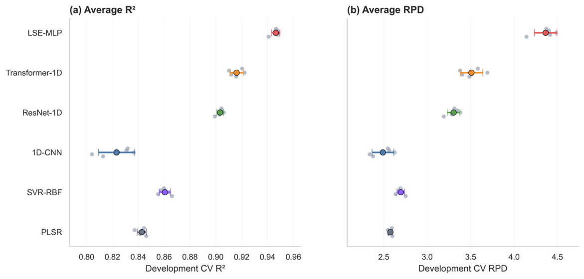
Under POINT_ID-grouped five-fold cross-validation, LSE-MLP achieved the highest R2 and RPD values for pH, OC, and N among the six evaluated models (Table 1). Its advantage was more pronounced for pH and N, whereas ResNet-1D and Transformer-1D also performed competitively for OC. The weaker performance of the evaluated 1D-CNN, particularly for pH and N, indicates that predictive accuracy varied substantially across the investigated neural architectures.
Table 1.
Property-specific prediction performance of the compared models under POINT_ID-grouped five-fold cross-validation on the development set.
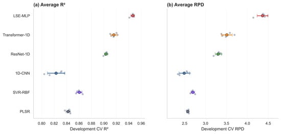
The fold-level distributions in Figure 4 show that LSE-MLP maintained the highest three-property average performance, with a generally consistent ranking of the main models across folds. These results suggest that the observed advantage was not confined to a single validation fold, although performance differences remained dependent on the evaluated model configurations and data partition.
Figure 4.
Prediction performance of the compared models under POINT_ID-grouped five-fold cross-validation on the development set. (a) Average R2 and (b) average RPD across the three target soil properties. Colored circles represent the mean across the five folds for each model, horizontal error bars indicate the standard deviation, and semi-transparent points denote the results of individual folds. Cross-validation was conducted only within the development set using POINT_ID as the grouping variable.
A supplementary paired POINT_ID-cluster bootstrap analysis further quantified the differences between LSE-MLP and the baseline models using development-set out-of-fold predictions. The pointwise 95% confidence intervals for ΔR2, ΔRMSE, and ΔMAE favored LSE-MLP across all 15 model–property comparisons (Table S12). These results provide additional evidence of performance differences under the evaluated cross-validation protocol, although the intervals do not account fully for retraining variability, alternative data partitions, or multiple-comparison uncertainty.
3.2. Results on the Independent Blind Test Set
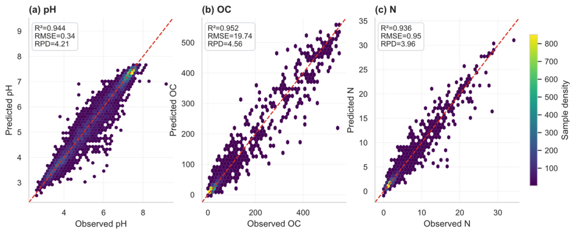
On the independent blind test set, LSE-MLP achieved the highest three-property average R2 among the evaluated models, with property-specific R2 values of 0.9437, 0.9519, and 0.9363 for pH, OC, and N, respectively (Table 2). The overall model ranking was broadly consistent with the development-set cross-validation results, with Transformer-1D and ResNet-1D remaining the strongest deep learning comparators. This consistency supports the performance of the selected LSE-MLP configuration on the held-out samples, without establishing generalization beyond the evaluated data source.
Table 2.
Property-specific prediction performance of the compared models on the independent blind test set.
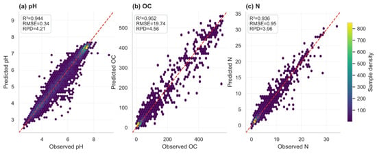
The observed-versus-predicted plots show that most LSE-MLP predictions were distributed near the 1:1 reference line (Figure 5). However, deviations remained for some samples with high OC values, indicating that strong aggregate accuracy did not eliminate property-specific prediction errors. Corresponding plots for the other models are provided in Figure S1.
Figure 5.
Property-specific predictions of LSE-MLP on the independent blind test set. (a) Soil pH; (b) organic carbon (OC); and (c) total nitrogen (N). The horizontal and vertical axes represent observed and predicted values, respectively. Point colors indicate local sample density, and the red dashed line denotes the 1:1 reference line. The corresponding R2, RMSE, and RPD values are reported in each panel.
3.3. Ablation and Stability Analyses of LSE-MLP
The ablation results indicate that spectral preprocessing contributed more strongly to predictive performance than the individual architectural modifications examined here (Table 3). Using raw spectra or SNV alone substantially reduced the average R2, whereas removing residual connections or replacing the learnable embedding with average pooling resulted in smaller decreases. These findings suggest that the selected preprocessing strategy and the combined embedding–regression architecture both contributed to performance, although their effects differed in magnitude.
Table 3.
Key ablation results of LSE-MLP under POINT_ID-grouped five-fold cross-validation on the development set.
The hyperparameter sensitivity analysis showed that moderate embedding dimensions and network depths provided favorable performance within the evaluated configurations (Table S3; Figure S2). Increasing model capacity did not consistently improve prediction accuracy, and the tested nonzero dropout settings offered no clear advantage. These results support the selected configuration within the investigated search space rather than establishing a globally optimal architecture.
Across five random seeds, LSE-MLP maintained higher average predictive performance and smaller seed-to-seed variation than ResNet-1D and Transformer-1D (Table S4; Figure S3). Its average R2 was 0.9443 ± 0.0021, indicating relatively consistent results under the evaluated training settings.
Across the three internal validation protocols, LSE-MLP maintained higher average R2 and RPD values than ResNet-1D and Transformer-1D (Table 4). The spatial-block split yielded slightly higher performance estimates than the POINT_ID-grouped and sample-level random splits. Because each protocol produced different training and validation subsets, this counterintuitive ordering may reflect differences in sample composition rather than the inherent difficulty of the partitioning strategies. The results therefore indicate relative consistency in model ranking under the evaluated splits, but do not establish stronger spatial generalization.
Table 4.
Model prediction performance under different internal validation protocols within the development set.
Training and validation loss curves for the four deep learning models, including fold-to-fold variation, are provided in Figure S4.
3.4. Computational Efficiency and Accuracy-Efficiency Trade-Off
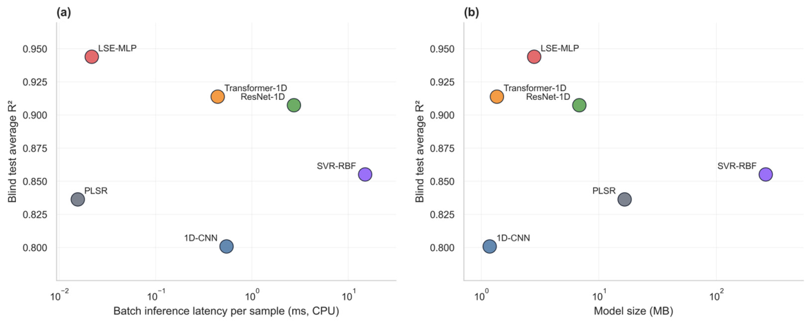
The computational comparison revealed different trade-offs between predictive accuracy, model storage, and inference cost (Table 5). LSE-MLP required approximately 1.47 MFLOPs per sample and achieved a Batch-128 CPU inference latency of 0.0217 ms per sample, while containing 736,899 parameters and occupying approximately 2.82 MB. Thus, its computational advantage among the evaluated deep learning models was reflected primarily in FLOPs and batch inference latency, rather than in the smallest parameter count or storage footprint.
Table 5.
Computational efficiency and resource costs of the evaluated models.
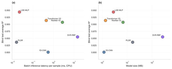
Considering predictive accuracy alongside computational cost, LSE-MLP occupied a favorable region of the accuracy–efficiency comparisons (Figure 6). Conventional models, particularly PLSR, could offer low inference latency but achieved lower predictive accuracy, whereas the stronger deep learning comparators generally required greater inference computation or latency. These findings support an accuracy–efficiency advantage under the evaluated CPU benchmarking conditions, without implying universally superior efficiency across hardware platforms.
Figure 6.
Accuracy–efficiency trade-offs among the evaluated models on the independent blind test set. (a) Average R2 versus Batch-128 per-sample CPU inference latency; and (b) average R2 versus model file size. Average R2 denotes the arithmetic mean of R2 values for pH, OC, and N. Each point represents one model, colors distinguish the evaluated models, and the horizontal axes are shown on logarithmic scales.
3.5. Spectral Importance Analysis Based on LSE Weights
The LSE weight-based importance profile showed a nonuniform distribution of model sensitivity across the spectrum, with relatively high values in parts of the near-infrared region and local peaks near 1400, 1900, 2200, and 2300 nm (Figure 7). These patterns identify spectral regions emphasized by the learned embedding but should not be interpreted as direct assignments to physical absorption mechanisms. Because the importance values were derived from model weights applied to preprocessed, highly correlated spectral variables, the analysis provides only an auxiliary characterization of model-level sensitivity.
Figure 7.
Wavelength importance derived from the linear spectral embedding weights of LSE-MLP. The light-blue curve represents the raw wavelength importance calculated from the absolute weights of the linear spectral embedding layer, whereas the dark-blue curve shows the smoothed overall trend. Orange regions identify wavelength positions within the top 2% of raw importance values. Gray dashed lines indicate reference wavelengths at approximately 1400, 1900, 2200, and 2300 nm. Importance values were normalized to the range of 0–1, and horizontal-axis wavelengths were approximately mapped from the input spectral features. The results reflect relative wavelength sensitivity at the embedding-weight level and should be interpreted only as auxiliary evidence.
3.6. Supplementary Analyses: Band Compression and External Data Applicability
To evaluate the performance of LSE-MLP under reduced input bands, this study conducted a continuous band-group compression experiment. The POINT_ID-grouped five-fold cross-validation results showed that the shared ranking strategy with 50% band-group retention maintained predictive performance close to that of full-spectrum LSE-MLP in terms of the overall average metrics, while reducing input size and computational cost (Table S5a,b). The multi-random-seed results showed that this strategy had small performance variation (Table S6). In addition, Figure S5 shows that certain contiguous band groups were selected more frequently across folds and random seeds, providing descriptive evidence of selection consistency. These selection frequencies should not, however, be interpreted as direct evidence of the physical importance of individual wavelengths.
After the final compression strategy was fixed, full-spectrum LSE-MLP and band-compressed LSE-MLP were further compared on the independent blind test set. For this compression experiment, the full-spectrum reference model was independently retrained rather than reused from the primary model comparison in Table 2. Although both full-spectrum evaluations used the same samples, model architecture, random seed, and principal training settings, they represented separate training runs and therefore yielded slightly different results. The band-compressed LSE-MLP maintained overall predictive performance close to that of its full-spectrum reference after reducing the number of input bands, while showing some advantages in FLOPs and CPU inference latency (Table S7a,b; Figure S6).
The data audit identified differences in property availability, sample size, and common wavelength coverage between KSSL and AUT (Table S8). Under within-dataset grouped five-fold cross-validation, LSE-MLP achieved R2 values of 0.9376 and 0.9679 for N and OC on KSSL, and 0.8460, 0.8088, and 0.8992 for N, OC, and pH on AUT, respectively (Table S9). In contrast, direct transfer of the frozen LUCAS-trained LSE-MLP yielded corresponding R2 values of −0.2391 and 0.0692 on KSSL, and −1.8075, −2.4232, and −2.3697 on AUT (Table S10). These results demonstrate a substantial difference between within-dataset modeling and direct cross-dataset transfer. Additional diagnostics revealed differences in target distributions and spectral characteristics, together with systematic prediction bias (Table S11; Figure S7).
4. Discussion
4.1. Complex Deep Models Are Not the Only Option for Soil Spectral Prediction
The results indicate that architectural complexity is not the sole determinant of predictive performance in soil Vis-NIR spectral regression. Previous studies using LUCAS data have highlighted the influence of spectral information, modeling strategies, and data characteristics on prediction accuracy [30]. In the present study, LSE-MLP achieved competitive performance by combining a learnable full-spectrum projection with residual nonlinear regression in a compact latent space. Its methodological contribution lies in this task-oriented representation and computation strategy, rather than in introducing fundamentally new neural network operations.
The effectiveness of this design may be associated with the distributed spectral information relevant to soil properties. By projecting all 4200 input variables into a lower-dimensional representation before nonlinear processing, LSE-MLP provides a computationally economical approach to multi-property regression. The sensitivity analysis further supports a moderate model capacity: an embedding dimension of 128 achieved the highest mean validation R2 among the evaluated settings, while increasing the residual depth from two to three blocks yielded only a marginal improvement (Table S3; Figure S2). These observations support the selected configuration within the investigated search space but do not establish its theoretical optimality.
These findings should not be interpreted as evidence that more complex architectures are generally unnecessary. Although consistent data partitions and evaluation procedures were adopted, differences in hyperparameter search spaces and training sample sizes limit the comparability of the evaluated models. In particular, the relatively weak performance of the 1D-CNN may partly reflect its specific architecture and optimization settings rather than an inherent limitation of convolutional approaches. Furthermore, the computational advantages of LSE-MLP are specific to the evaluated hardware and inference conditions. Therefore, LSE-MLP should be regarded as a practical option offering a favorable accuracy–efficiency trade-off under the investigated conditions, rather than a universally superior architecture.
4.2. Model Evaluation Should Not Be Limited to Predictive Accuracy
Soil spectral data may contain repeated sampling points, spatial clustering, and regional similarity. Therefore, predictive accuracy under a single data partition may not fully represent model performance. The three internal validation protocols used in this study produced different performance estimates, with the spatial-block split yielding slightly higher predictive accuracy than the random and POINT_ID-grouped splits. This counterintuitive result may reflect differences in the composition of the training and validation subsets, including soil-property distributions, spectral characteristics, and spatial coverage, rather than an inherent difference in the difficulty of the validation protocols. However, these potential contributing factors were not independently quantified, and the observed result should not be interpreted as evidence that spatially separated validation is generally easier or that LSE-MLP has stronger spatial transferability. Accordingly, the comparison is best regarded as an assessment of sensitivity to data partitioning rather than a definitive ranking of validation protocols by difficulty.
Predictive accuracy should also be interpreted in relation to model architecture. The ablation experiments showed that the predictive performance of LSE-MLP resulted from the combined effects of spectral preprocessing, full-spectrum embedding, and nonlinear modeling. Removing or replacing these components led to varying degrees of performance decrease, indicating that the current combined design was suitable for the task examined in this study.
Model evaluation should also consider computational cost and potential deployment conditions. The lightweight nature of LSE-MLP was mainly reflected in the low computational cost of its inference path, rather than in minimizing the number of parameters or model file size. The band compression experiment showed that, without changing the main architecture, continuous band-group compression could serve as a supplementary strategy for reducing input size and supporting the accuracy–efficiency trade-off. However, the reported CPU inference latency reflects the original benchmarking conditions, for which the thread configuration and software versions were not fully recorded. Real-world deployment performance may also depend on hardware resources, inference frameworks, energy constraints, and data transfer conditions [31].
4.3. Model Interpretation and Application Boundaries
The LSE weight analysis provides an auxiliary indication of the spectral regions to which the trained model is relatively sensitive. The observed weight distribution was nonuniform across the spectrum, suggesting that different spectral regions contributed differently to the learned representation. However, these weights reflect statistical relationships learned from the preprocessed spectral inputs rather than the independent physical contributions of individual wavelengths. In particular, the strong correlation among adjacent spectral variables and the use of SNV transformation followed by the Savitzky–Golay first derivative complicate direct physical interpretation. Therefore, peaks in the LSE weight profile should not be equated with absorption peaks in the original reflectance spectra or treated as evidence of specific soil chemical mechanisms. The analysis is intended to characterize model-level spectral sensitivity rather than establish physical causality.
The external dataset results highlight the distinction between within-dataset prediction and direct cross-dataset transfer. The marked deterioration in the R2 values of frozen LUCAS-trained models suggests limited transferability under the evaluated conditions. Several factors may contribute to this outcome. First, differences in spectral coverage, particularly the absence of wavelengths below 680 nm in AUT, may alter the available predictive information. Second, variations in instruments, acquisition procedures, and laboratory measurement protocols may affect spectral and target consistency, even after wavelength and unit harmonization. Previous studies have also highlighted the influence of data sources, measurement scenarios, and auxiliary information on soil spectral prediction [32,33]. Third, the observed differences in soil-property distributions, spectral-domain characteristics, and prediction bias (Table S11; Figure S7) suggest substantial dataset heterogeneity. However, the individual contributions of these factors were not isolated experimentally. Moreover, grouped validation on KSSL and AUT used unique layer identifiers rather than geographic locations and should not be interpreted as strict spatial validation. Environmental factors, such as soil moisture, may further influence Vis-NIR predictive performance under field conditions [34]. These findings indicate that successful within-dataset modeling does not guarantee reliable cross-dataset transfer without further calibration and independent validation.
This study has several limitations. First, the primary experiments were based on LUCAS2009, which mainly represents European topsoil samples. Although KSSL and AUT were included as external datasets, the observed direct-transfer degradation indicates that geographical generalization and cross-instrument robustness remain insufficiently established. Differences in spectral domains, soil-property distributions, and measurement protocols further limit the transferability of the trained models. Second, although previous research has demonstrated the potential of infrared spectroscopy for predicting additional soil indicators [35], the present study considered only pH, OC, and N. Therefore, the applicability of LSE-MLP to other soil properties, such as cation exchange capacity, clay, silt, and sand, remains to be evaluated. Third, the experiments relied on existing laboratory spectral datasets, while the efficiency measurements were obtained under controlled CPU benchmarking conditions. Consequently, model robustness under real field conditions, including variable soil moisture, surface characteristics, illumination, and portable-instrument constraints, has not been demonstrated. Further validation across regions, instruments, laboratories, and field-measurement conditions is required.
Future studies could introduce more independent data sources and soil properties, and combine systematic interpretability analysis with real hardware testing to evaluate the reliability of lightweight full-spectrum models under different data conditions and application scenarios. Deep model visualization and interpretable machine learning methods can provide reference information for analyzing model-sensitive regions [36,37], but such interpretations should still be assessed together with soil spectral knowledge and independent validation.
5. Conclusions
This study developed and evaluated LSE-MLP, a lightweight full-spectrum embedding model that uses soil Vis-NIR spectra as input to simultaneously predict pH, OC, and N. Based on a unified comparison using the LUCAS2009 dataset, LSE-MLP achieved competitive predictive performance under both POINT_ID-grouped cross-validation and independent blind test set evaluation. The ablation experiments showed that SNV transformation combined with the Savitzky–Golay first derivative, learnable linear spectral embedding, and the residual MLP structure jointly supported model performance. The efficiency analysis indicated that the lightweight characteristics of LSE-MLP were mainly reflected in lower FLOPs and faster batch CPU inference latency, rather than in having the fewest parameters or the smallest model file size.
The supplementary experiments indicated that continuous band-group compression could reduce spectral input dimensionality while maintaining predictive performance close to that of the full-spectrum model under the investigated conditions. External evaluations on KSSL and AUT demonstrated that competitive within-dataset performance did not guarantee reliable direct transfer of LUCAS-trained models. This finding highlights the practical need for dataset-specific validation and, where necessary, calibration adaptation before applying the model to new soil populations or measurement systems. Overall, LSE-MLP provides a practical accuracy–efficiency option for soil Vis-NIR regression within the evaluated settings, while broader geographical generalization, cross-instrument robustness, and field deployment require further investigation.
Supplementary Materials
The following supporting information can be downloaded at: https://www.mdpi.com/article/10.3390/sym18111821/s1, Table S1: Descriptive statistics of the target soil properties in the LUCAS2009 dataset; Table S2: Evaluated hyperparameter candidates and final selected settings of the compared models; Table S3: Hyperparameter sensitivity analysis of LSE-MLP; Table S4: Multi-random-seed stability comparison of the deep learning models; Table S5: Predictive performance and computational efficiency of band-compression strategies; Table S6: Multi-random-seed stability of the shared ranking 50% band-compression strategy; Table S7: Predictive performance and computational efficiency of full-spectrum and band-compressed LSE-MLP; Table S8: Audit results and comparability information for the external soil spectral datasets; Table S9: Predictive performance of different models under internal five-fold cross-validation on the KSSL and AUT datasets; Table S10: Direct transfer performance of frozen LUCAS-trained models on KSSL and AUT; Table S11: Target-distribution differences, spectral-domain shifts, and LSE-MLP systematic bias diagnostics between LUCAS and the external datasets; Table S12: Paired POINT_ID-cluster bootstrap confidence intervals for differences in predictive performance between LSE-MLP and baseline models under development-set five-fold cross-validation; Figure S1: Comparison of observed and predicted soil properties for different models on the independent blind test set; Figure S2: Hyperparameter sensitivity of LSE-MLP under POINT_ID-grouped five-fold cross-validation on the development set; Figure S3: Multi-random-seed prediction stability of the evaluated deep learning models; Figure S4: Convergence curves of the deep learning models during POINT_ID-grouped five-fold cross-validation on the development set; Figure S5: Selection frequency of contiguous band groups under the shared ranking 50% band-compression strategy; Figure S6: Accuracy–efficiency comparison between full-spectrum and band-compressed LSE-MLP on the independent blind test set; Figure S7: Spectral-domain and target-distribution differences between LUCAS and the external datasets.
Author Contributions
Conceptualization, X.C., M.D. and Y.W.; methodology, M.D. and Y.W.; software, M.D.; validation, M.D., Y.D. and Q.L.; formal analysis, M.D.; investigation, M.D. and Y.D.; resources, X.C. and Y.W.; data curation, M.D.; writing—original draft preparation, M.D.; writing—review and editing, X.C., Y.W., Y.D. and Q.L.; visualization, M.D.; supervision, X.C. and Y.W.; project administration, X.C. and Y.W.; funding acquisition, X.C. and Y.W. All authors have read and agreed to the published version of the manuscript.
Funding
This research work was supported by Key R & D projects of Guangxi Science and Technology Program (Guike.AB24010338), Guangxi Regional Innovation Capacity Enhancement Program Project (GuiKe XT2503960041), Independent research project (GXRDCF202307-01).
Data Availability Statement
The datasets analyzed in this study are available from public data sources. The LUCAS2009 topsoil data are available from the European Soil Data Centre (ESDAC) at https://esdac.jrc.ec.europa.eu/content/lucas-2009-topsoil-data (accessed on 5 November 2025). The KSSL data are available from the USDA National Cooperative Soil Survey Lab Data Mart at https://ncsslabdatamart.sc.egov.usda.gov/ (accessed on 28 June 2026). The Austrian Near-Infrared (NIR) Soil Spectral Library (AUT) is available at https://docs.soilspectroscopy.org/datasets/AUT.html (accessed on 28 June 2026).
Conflicts of Interest
The authors declare no conflicts of interest.
Abbreviations
The following abbreviations are used in this manuscript:
| AUT | Austrian Near-Infrared (NIR) Soil Spectral Library |
| CEC | Cation exchange capacity |
| CPU | Central processing unit |
| FLOPs | Floating-point operations |
| KSSL | Kellogg Soil Survey Laboratory |
| LSE | Linear spectral embedding |
| LSE-MLP | Lightweight full-spectrum embedding multilayer perceptron |
| LUCAS | Land Use and Coverage Area frame Survey |
| MAE | Mean absolute error |
| MLP | Multilayer perceptron |
| N | Total nitrogen |
| OC | Organic carbon |
| PLSR | Partial least squares regression |
| RBF | Radial basis function |
| RMSE | Root mean squared error |
| RPD | Ratio of performance to deviation |
| SG-1D | Savitzky–Golay first derivative |
| SNV | Standard normal variate |
| SVR | Support vector regression |
| Vis-NIR | Visible–near-infrared |
| 1D-CNN | One-dimensional convolutional neural network |
References
- Liakos, K.; Busato, P.; Moshou, D.; Pearson, S.; Bochtis, D. Machine Learning in Agriculture: A Review. Sensors 2018, 18, 2674. [Google Scholar] [CrossRef] [Scilit] [PubMed]
- Ahmadi, A.; Emami, M.; Daccache, A.; He, L. Soil Properties Prediction for Precision Agriculture Using Visible and Near-Infrared Spectroscopy: A Systematic Review and Meta-Analysis. Agronomy 2021, 11, 433. [Google Scholar] [CrossRef] [Scilit]
- Ge, Y. A Primer on Soil Analysis Using Visible and Near-Infrared (Vis-NIR) and Mid-Infrared (MIR) Spectroscopy; Soil Spectroscopy Training Manual; FAO: Rome, Italy, 2022; ISBN 978-92-5-135898-6. [Google Scholar]
- Piccini, C.; Metzger, K.; Debaene, G.; Stenberg, B.; Götzinger, S.; Borůvka, L.; Sandén, T.; Bragazza, L.; Liebisch, F. In-Field Soil Spectroscopy in Vis–NIR Range for Fast and Reliable Soil Analysis: A Review. Eur. J. Soil Sci. 2024, 75, e13481. [Google Scholar] [CrossRef] [Scilit]
- Shin, S.K.; Lee, S.J.; Park, J.H. Prediction of Soil Properties Using Vis-NIR Spectroscopy Combined with Machine Learning: A Review. Sensors 2025, 25, 5045. [Google Scholar] [CrossRef] [Scilit] [PubMed]
- Hateffard, F.; Gumbricht, T.; Ranhem, T.; Breure, T.; Panagos, P.; Hugelius, G. Predicting Soil Properties Using Spectral Subsets of LUCAS Visible Near-Infrared Spectroscopy Data. Eur. J. Soil Sci. 2025, 76, e70242. [Google Scholar] [CrossRef] [Scilit]
- Ng, W.; Minasny, B.; Montazerolghaem, M.; Padarian, J.; Ferguson, R.; Bailey, S.; McBratney, A.B. Convolutional Neural Network for Simultaneous Prediction of Several Soil Properties Using Visible/near-Infrared, Mid-Infrared, and Their Combined Spectra. Geoderma 2019, 352, 251–267. [Google Scholar] [CrossRef] [Scilit]
- Yang, J.; Wang, X.; Wang, R.; Wang, H. Combination of Convolutional Neural Networks and Recurrent Neural Networks for Predicting Soil Properties Using Vis–NIR Spectroscopy. Geoderma 2020, 380, 114616. [Google Scholar] [CrossRef] [Scilit]
- Cao, L.; Sun, M.; Yang, Z.; Jiang, D.; Yin, D.; Duan, Y. A Novel Transformer-CNN Approach for Predicting Soil Properties from LUCAS Vis-NIR Spectral Data. Agronomy 2024, 14, 1998. [Google Scholar] [CrossRef] [Scilit]
- Ke, Z.; Ren, S.; Yin, L. Advancing Soil Property Prediction with Encoder-Decoder Structures Integrating Traditional Deep Learning Methods in Vis-NIR Spectroscopy. Geoderma 2024, 449, 117006. [Google Scholar] [CrossRef] [Scilit]
- Jin, X.; Zhou, J.; Rao, Y.; Zhang, X.; Zhang, W.; Ba, W.; Zhou, X.; Zhang, T. An Innovative Approach for Integrating Two-Dimensional Conversion of Vis-NIR Spectra with the Swin Transformer Model to Leverage Deep Learning for Predicting Soil Properties. Geoderma 2023, 436, 116555. [Google Scholar] [CrossRef] [Scilit]
- Padarian, J.; Minasny, B.; McBratney, A.B. Using Deep Learning to Predict Soil Properties from Regional Spectral Data. Geoderma Reg. 2019, 16, e00198. [Google Scholar] [CrossRef] [Scilit]
- Zhai, Z.; Chen, F.; Yu, H.; Hu, J.; Zhou, X.; Xu, H. PS-MTL-LUCAS: A Partially Shared Multi-Task Learning Model for Simultaneously Predicting Multiple Soil Properties. Ecol. Inform. 2024, 82, 102784. [Google Scholar] [CrossRef] [Scilit]
- Padarian, J.; Minasny, B.; McBratney, A.B. Transfer Learning to Localise a Continental Soil Vis-NIR Calibration Model. Geoderma 2019, 340, 279–288. [Google Scholar] [CrossRef] [Scilit]
- Schwartz, R.; Dodge, J.; Smith, N.A.; Etzioni, O. Green AI. Commun. ACM 2020, 63, 54–63. [Google Scholar] [CrossRef] [Scilit]
- Wang, X.; Zhang, M.-W.; Zhou, Y.-N.; Wang, L.; Zeng, L.-T.; Cui, Y.-P.; Sun, X.-L. Simultaneous Estimation of Multiple Soil Properties from Vis-NIR Spectra Using a Multi-Gate Mixture-of-Experts with Data Augmentation. Geoderma 2025, 453, 117127. [Google Scholar] [CrossRef] [Scilit]
- Wang, H.; Sun, Q.; Niu, X.; Liu, K.; Zhang, J.; Hao, Z.; Xu, D. Soil Organic Carbon Prediction Using an Efficient Channel Attention-Enhanced CNN-LSTM Model With LUCAS Spectral Library. Eur. J. Soil Sci. 2025, 76, e70202. [Google Scholar] [CrossRef] [Scilit]
- Li, C.; Song, L.; Zheng, L.; Ji, R. DSCformer: Lightweight Model for Predicting Soil Nitrogen Content Using VNIR-SWIR Spectroscopy. Comput. Electron. Agric. 2025, 230, 109761. [Google Scholar] [CrossRef] [Scilit]
- Meyer, H.; Reudenbach, C.; Hengl, T.; Katurji, M.; Nauss, T. Improving Performance of Spatio-Temporal Machine Learning Models Using Forward Feature Selection and Target-Oriented Validation. Environ. Model. Softw. 2018, 101, 1–9. [Google Scholar] [CrossRef] [Scilit]
- Meyer, H.; Pebesma, E. Predicting into Unknown Space? Estimating the Area of Applicability of Spatial Prediction Models. Methods Ecol. Evol. 2021, 12, 1620–1633. [Google Scholar] [CrossRef] [Scilit]
- Orgiazzi, A.; Ballabio, C.; Panagos, P.; Jones, A.; Fernández-Ugalde, O. LUCAS Soil, the Largest Expandable Soil Dataset for Europe: A Review. Eur. J. Soil Sci. 2018, 69, 140–153. [Google Scholar] [CrossRef] [Scilit]
- Deiss, L.; Margenot, A.J.; Culman, S.W.; Demyan, M.S. Tuning Support Vector Machines Regression Models Improves Prediction Accuracy of Soil Properties in MIR Spectroscopy. Geoderma 2020, 365, 114227. [Google Scholar] [CrossRef] [Scilit]
- Wang, Z.; Chen, S.; Lu, R.; Zhang, X.; Ma, Y.; Shi, Z. Non-Linear Memory-Based Learning for Predicting Soil Properties Using a Regional Vis-NIR Spectral Library. Geoderma 2024, 441, 116752. [Google Scholar] [CrossRef] [Scilit]
- Vestergaard, R.-J.; Vasava, H.B.; Aspinall, D.; Chen, S.; Gillespie, A.; Adamchuk, V.; Biswas, A. Evaluation of Optimized Preprocessing and Modeling Algorithms for Prediction of Soil Properties Using VIS-NIR Spectroscopy. Sensors 2021, 21, 6745. [Google Scholar] [CrossRef] [Scilit] [PubMed]
- Guo, P.; Li, T.; Gao, H.; Chen, X.; Cui, Y.; Huang, Y. Evaluating Calibration and Spectral Variable Selection Methods for Predicting Three Soil Nutrients Using Vis-NIR Spectroscopy. Remote Sens. 2021, 13, 4000. [Google Scholar] [CrossRef] [Scilit]
- Zhang, X.; Xue, J.; Xiao, Y.; Shi, Z.; Chen, S. Towards Optimal Variable Selection Methods for Soil Property Prediction Using a Regional Soil Vis-NIR Spectral Library. Remote Sens. 2023, 15, 465. [Google Scholar] [CrossRef] [Scilit]
- Lei, T.; Sun, D.-W. Achieving Joint Calibration of Soil Vis-NIR Spectra across Instruments, Soil Types and Properties by an Attention-Based Spectra Encoding-Spectra/Property Decoding Architecture. Geoderma 2022, 405, 115449. [Google Scholar] [CrossRef] [Scilit]
- de Sousa Mendes, W.; Sommer, M.; Koszinski, S.; Wehrhan, M. Peatlands Spectral Data Influence in Global Spectral Modelling of Soil Organic Carbon and Total Nitrogen Using Visible-near-Infrared Spectroscopy. J. Environ. Manag. 2022, 317, 115383. [Google Scholar] [CrossRef] [Scilit] [PubMed]
- Yang, M.; Chen, S.; Xu, D.; Hong, Y.; Li, S.; Peng, J.; Ji, W.; Guo, X.; Zhao, X.; Shi, Z. Strategies for Predicting Soil Organic Matter in the Field Using the Chinese Vis-NIR Soil Spectral Library. Geoderma 2023, 433, 116461. [Google Scholar] [CrossRef] [Scilit]
- Liu, B.; Guo, B.; Zhuo, R.; Dai, F. Estimation of Soil Organic Carbon in LUCAS Soil Database Using Vis-NIR Spectroscopy Based on Hybrid Kernel Gaussian Process Regression. Spectrochim. Acta Part A Mol. Biomol. Spectrosc. 2024, 321, 124687. [Google Scholar] [CrossRef] [Scilit] [PubMed]
- Ahmad, S.; Shakeel, I.; Mehfuz, S.; Ahmad, J. Deep Learning Models for Cloud, Edge, Fog, and IoT Computing Paradigms: Survey, Recent Advances, and Future Directions. Comput. Sci. Rev. 2023, 49, 100568. [Google Scholar] [CrossRef] [Scilit]
- Kodaira, M.; Shibusawa, S. Mobile Proximal Sensing with Visible and Near Infrared Spectroscopy for Digital Soil Mapping. Soil Syst. 2020, 4, 40. [Google Scholar] [CrossRef] [Scilit]
- Kok, M.; Sarjant, S.; Verweij, S.; Vaessen, S.F.C.; Ros, G.H. On-Site Soil Analysis: A Novel Approach Combining NIR Spectroscopy, Remote Sensing and Deep Learning. Geoderma 2024, 446, 116903. [Google Scholar] [CrossRef] [Scilit]
- Xie, A.; Wu, W. Evaluating the Impact of Soil Moisture Variation on the Performance of Visible and Near-Infrared (Vis–NIR) Spectroscopy for Predicting Soil Organic Carbon Content. Environ. Monit. Assess. 2025, 197, 1221. [Google Scholar] [CrossRef] [Scilit] [PubMed]
- Irving, D.; Tran, T.K.A.; Poudel, S.; Tang, Y.; Ng, W.; Xue, P.; McBratney, A.B.; Minasny, B. Infrared Spectroscopy Prediction of Soil Microbial Properties across Australian Soils: Drivers and Limitations. Soil Environ. Health 2026, 4, 100205. [Google Scholar] [CrossRef] [Scilit]
- Selvaraju, R.R.; Cogswell, M.; Das, A.; Vedantam, R.; Parikh, D.; Batra, D. Grad-CAM: Visual Explanations from Deep Networks via Gradient-Based Localization. Int. J. Comput. Vis. 2020, 128, 336–359. [Google Scholar] [CrossRef] [Scilit]
- Hu, Y.; Viscarra Rossel, R.A. Estimating Soil Carbon Sequestration Potential with Mid-IR Spectroscopy and Explainable Machine Learning. Soil 2026, 12, 619–631. [Google Scholar] [CrossRef] [Scilit]

Disclaimer/Publisher’s Note: The statements, opinions and data contained in all publications are solely those of the individual author(s) and contributor(s) and not of MDPI and/or the editor(s). MDPI and/or the editor(s) disclaim responsibility for any injury to people or property resulting from any ideas, methods, instructions or products referred to in the content. |
© 2026 by the authors. Licensee MDPI, Basel, Switzerland. This article is an open access article distributed under the terms and conditions of the Creative Commons Attribution (CC BY) license.