


Abstract
Transparent curved surfaces of glass packaging bottles produce structural responses that can obscure local appearance asymmetries associated with defects, complicating their segmentation across different scales and shapes. To address these challenges, we propose DFSR-Net, a glass bottle defect segmentation network. A Differential Context Modulation Module combines local differential responses with multiscale context to enhance weak anomalies while suppressing interference from normal bottle structures. A Key-Node Sparse Graph Propagation module uses key-node selection and restricted neighborhood aggregation to limit irrelevant cross-layer propagation and selectively transfer informative defect features. In the decoder, Dual-Receptive-Field Spatial Selection adaptively integrates local details and broader context, while Dual-Statistic Directional Calibration calibrates height- and width-wise spatial responses to improve region completeness and boundary representation. Experiments on the public Bottle Body dataset and the self-collected industrial glass bottle defect dataset show that DFSR-Net achieves mean Intersection over Union values of 81.08% and 80.14%. DFSR-Net also achieves a single-image processing speed of 74.3 FPS while maintaining high segmentation accuracy, suggesting potential for online glass bottle defect inspection.
1. Introduction
Glass packaging bottles are widely used for food, pharmaceutical, and other products because of their good chemical stability and barrier properties. Variations in manufacturing processes and subsequent mechanical stresses may cause various surface or structural defects during production and transportation. These defects not only degrade the appearance quality of the products but, in severe cases, may also compromise the structural integrity and service reliability of the bottles [1,2]. Conventional manual sampling inspection is limited by low inspection efficiency and subjective judgment, making it increasingly difficult to meet the requirements of continuous quality control on high-speed production lines. With the development of industrial machine vision, image-based automated defect inspection has gradually become an important approach to quality control for glass packaging [3]. Therefore, developing high-accuracy vision-based inspection methods for glass packaging bottles is important for improving automated quality control in manufacturing processes.
Many glass packaging bottles have approximately rotationally symmetric geometries, yet their transparent curved surfaces produce imaging characteristics that differ from those of conventional opaque industrial surfaces. Local defects may disrupt the regular appearance of bottle walls, while refraction and illumination can produce nonuniform responses even in defect-free regions. Under transmission or backlighting conditions, variations in bottle-wall curvature and thickness alter the light propagation path, producing pronounced intensity transitions and strong edge responses around the bottle mouth, shoulder, and outer contour. These structural responses reduce the distinction between weak defects and normal regions, making defects that appear only as local transmittance variations or texture anomalies more likely to be obscured by the background. Meanwhile, curved-surface projection changes the appearance of defects in two-dimensional images, causing their scale, elongation direction, and boundary shape to vary with spatial location. Different types of defects also exhibit distinct spatial distributions, further increasing the risk of missed detections and incorrect segmentation. Therefore, fine-grained identification of glass packaging bottle defects requires not only distinguishing and preserving weak anomaly information from complex structural responses of the bottle, but also jointly considering local details and broader structural relationships to accurately characterize the shape and boundary variations of defect regions.
Given the above imaging characteristics, relying only on category classification or coarse localization is insufficient to fully describe the actual shape of defect regions, whereas pixel-level segmentation can directly characterize the spatial extent and boundary variations of abnormal regions, making it more suitable for fine-grained identification of glass packaging bottle defects. Versini et al. [4] applied pixel-level segmentation to glass bottle surface defect detection and incorporated classification information to improve the recognition of abnormal regions. As research on defect segmentation has progressed, multiscale information supplementation and cross-layer feature interaction have been increasingly used to alleviate detail loss during encoding. Cheng et al. [5] employed pyramid adaptive selection to supplement fine-grained features at different levels and introduced cross-attention to improve information fusion between the encoder and decoder. Such cross-layer collaboration enhances the complementarity of information across different scales. However, under complex backgrounds, inter-level information transfer alone remains insufficient to fully characterize the spatial relationships between defects and surrounding structures. To address this issue, Bian et al. [6] combined local perception with global context modeling, establishing broader spatial associations while preserving fine-grained responses and thereby improving the region representation of small defects in complex backgrounds. As the range of feature interaction expands, irrelevant background information is more likely to participate in feature interaction, placing higher demands on effective feature selection. Tian et al. [7] used global context to guide feature selection, reducing the interference of complex textures with tiny-defect representation and further improving the selective utilization of contextual information. Nevertheless, when defect scales and spatial shapes vary, a unified feature aggregation strategy still struggles to accommodate the structural representation requirements of different regions.
Despite continued advances in detail recovery, cross-layer fusion, and contextual modeling, existing methods still struggle to fully address the imaging characteristics of glass packaging bottles with transparent curved surfaces. Specifically, local feature enhancement may amplify strong normal responses, such as bottle contours and refractive boundaries, while enhancing weak anomalies. Cross-layer interaction can supplement shallow details, but it may also propagate structural interference together with informative features. In addition, fixed feature aggregation strategies are difficult to adapt to the differences in spatial representation among defects with different locations and shapes. Therefore, how to selectively enhance weak defect responses, restrict the cross-layer propagation of irrelevant information, and improve the structural representation of defects with different spatial characteristics remains a key issue for improving glass packaging bottle defect segmentation.
Based on the above analysis, we develop a defect segmentation network for glass packaging bottles with transparent curved surfaces to improve defect representation under complex imaging conditions through three aspects: weak anomaly enhancement, cross-layer information transfer, and spatial structure reconstruction. The main contributions are summarized as follows:
- (1)
- To address the confusion between weak defect responses and strong normal structural responses of the bottle, we propose a Differential Context Modulation Module (DCMM). By jointly modeling local differential responses and multiscale contextual information, DCMM enhances weak defect features while suppressing excessive responses from normal bottle structures.
- (2)
- We design a Key-Node Sparse Graph Propagation (KSGP) module to suppress the propagation of irrelevant structural information during cross-layer feature transfer between the encoder and decoder. Through importance-based node selection and restricted neighborhood aggregation, KSGP enables the selective transfer of informative defect features.
- (3)
- To address the differences in spatial representation among defects with different locations and shapes, we jointly regulate the feature aggregation range and directional spatial relationships in the decoder. Specifically, the Dual-Receptive-Field Spatial Selection (DRSS) module dynamically fuses local details with broader contextual information, while the Dual-Statistic Directional Calibration (DSDC) module calibrates spatial responses along the height and width directions, thereby improving the continuity of defect regions and their boundary representation.
2. Related Work
Quality inspection of transparent glass containers involves not only defect recognition and localization, as commonly studied in industrial vision, but also the challenges introduced by transparent curved-surface imaging, which place higher demands on fine-grained representation of abnormal regions. With the development of vision-based inspection techniques, related studies have gradually progressed from defect classification and region localization to pixel-level segmentation, with increasing attention to the roles of multiscale features, hierarchical information, and contextual relationships in defect representation. Following this progression, this section reviews research closely related to glass packaging bottle defect inspection.
2.1. Defect Detection in Glass Containers
Early studies on glass container defect detection mainly focused on anomaly identification within specific regions or from particular viewing angles. With the development of deep vision methods, research has gradually extended to the joint determination of defect categories and spatial locations. Phalawan et al. [8] combined weakly supervised learning with multi-view analysis and exploited complementary information across different views to improve the robustness of glass bottle defect recognition, alleviating the problem of incomplete anomaly information from a single view. Tomita et al. [9] addressed the complex structure of bottle mouths and the interference caused by normal textures by first extracting effective inspection regions and then performing defect classification, allowing the recognition process to focus more closely on critical regions. These studies improved anomaly recognition in specific scenarios, but their ability to describe the spatial location and regional shape of defects remained limited. To obtain more explicit defect locations, Xu et al. [10] applied an improved YOLOv5s to glass bottle surface defect detection, enabling simultaneous prediction of defect categories and locations. However, rectangular bounding boxes mainly provide a coarse description of abnormal regions and have limited capability to represent the actual boundaries of elongated or irregular defects. Zhang et al. [11] further integrated edge information and contextual features to enhance the representation of ambiguous defects and introduced a scale-aware localization strategy to improve defect localization accuracy under complex conditions. Nevertheless, the detection results are still mainly represented by bounding boxes, making it difficult to fully describe the actual regions and boundaries of defects.
For cracks, stripe-like anomalies, and irregular defects, rectangular bounding boxes alone are insufficient to fully represent their actual spatial shapes. Versini et al. [4] apply pixel-level segmentation to glass bottle surface defect detection and incorporate classification information to assist segmentation prediction, enabling the detection results to further delineate defect regions and boundaries. Existing studies have gradually progressed from anomaly identification and object localization toward more fine-grained region description. However, under transparent curved-surface imaging conditions, weak defects coexist with strong responses from normal structures, while different defects also exhibit substantial variations in scale and boundary shape. Therefore, further improvements are still needed in preserving weak anomaly information and accurately reconstructing complex defect regions.
2.2. Surface Defect Segmentation Methods
Pixel-level segmentation of surface defects requires not only the identification of abnormal regions but also the preservation of fine-grained information, such as defect boundaries and local shapes. Continuous downsampling tends to weaken the local responses of small-scale and low-contrast defects. Therefore, recent studies increasingly employ multiscale features and attention mechanisms to compensate for detail loss during encoding. Huang et al. [12] introduce a multiscale feature extraction module in EDSV-Net and employ spatial and channel attention to enhance low-level spatial information and high-level semantic features, respectively, thereby improving the representation of defects at different scales. Chen et al. [13] propose A-Net, which coordinates low-level details and high-level semantic information through an A-shaped lightweight encoder–decoder architecture and employs lightweight feature extraction units to reduce computational cost while maintaining real-time defect segmentation performance. These methods enhance responses in informative regions, but their enhancement criteria mainly rely on feature saliency and lack an explicit distinction between defect responses and high-response structures in complex backgrounds. Cheng et al. [5] further introduce a pyramid adaptive selection module that incorporates features at different resolutions into the encoding process and selects hierarchical information according to feature responses, alleviating the loss of fine-grained information caused by continuous encoding. Although feature selection reduces some redundant information, high responses do not necessarily correspond to actual defects. When strong edges, regular textures, or local structural variations are present in the background, these regions may still receive high weights, making it difficult to directly suppress structural interference during feature enhancement.
Building on multiscale detail enhancement, expanding the receptive field helps exploit structural relationships around defects. Tang et al. [14] employ multiscale dilated convolutions in PUNet to enlarge the receptive field and combine polarized self-attention to enhance small-scale defects in low-contrast backgrounds. Li et al. [15] further integrate multiscale feature fusion with a multiscale attention decoder in MFF-Metal and use knowledge distillation to reduce the model size, allowing features from different levels and receptive ranges to participate in defect region reconstruction. Multiscale contextual information can supplement local features, but a larger receptive field also introduces more background responses, while attention-based reweighting alone still lacks explicit constraints on the relationship between abnormal regions and surrounding structures. Bian et al. [6] combine local perception with visual state-space modeling to preserve local responses while establishing broader-range dependencies, and further employ multidirectional scanning to enhance the representation of small defects in complex backgrounds. Such broader-range information interaction alleviates the limitation of modeling local features in isolation, but background structures may also enter the feature propagation process as the interaction range expands, which can still weaken the discriminability of weak defects when high-response background regions occupy a large proportion of the image. Zhang et al. [16] further employ a dual-branch architecture based on CNNs and global self-attention to jointly model local details and long-range relationships, and strengthen their interaction through cross-branch information exchange. Although the joint use of local and global features improves the structural representation of complex defects, the design still mainly focuses on fusing information from different ranges and lacks direct constraints on the differences between normal structural responses and weak anomalies.
Existing methods mainly strengthen feature responses through multiscale information supplementation, attention-based selection, or contextual aggregation. However, when bottle contours and refractive boundaries also exhibit strong local variations, structural interference may be enhanced together with informative features. To address this issue, we design DCMM to constrain feature enhancement using local differences and surrounding structural information, thereby strengthening weak defect features while reducing interference from normal bottle structures. This design improves the representation of weak defect regions and the accuracy of boundary recovery.
2.3. Hierarchical Feature Modeling Strategy
The performance of surface defect segmentation depends not only on the discriminative capability of features at individual levels, but also on how information from different levels is transferred, complemented, and reorganized during defect region reconstruction. With the development of encoder–decoder networks, the joint utilization of shallow details and high-level semantics has evolved from direct skip connections to more flexible hierarchical feature modeling strategies, including attention guidance, adaptive weighting, and contextual modeling. By strengthening the interaction among features at different levels and further coordinating local information with broader contextual relationships, these methods provide richer feature representations for recovering defect details and modeling spatial structures.
In cross-layer information transfer, direct concatenation or element-wise addition can supplement shallow details, but may also introduce semantic discrepancies and redundant responses between different feature levels into the decoding process. As this issue has received increasing attention, cross-layer fusion has gradually shifted from indiscriminate feature transfer toward adaptive regulation of feature contributions. Zhang et al. [17] employ context-aware weighting in CAWANet to suppress deep-layer noise while recovering details lost during decoding. Xiao et al. [18] introduce learnable gating in WFF-Net to assign fusion weights according to the effectiveness of features at different levels, thereby reducing semantic discrepancies and information redundancy between low- and high-level features. Guo et al. [19] further employ a task-specific decoding structure and metric constraints to enable shared encoder features to be selectively utilized according to different reconstruction requirements. Luo et al. [20] combine a feature pyramid with attention interaction to strengthen the connections between multiscale encoder and decoder features. Li et al. [21] further propose OCINet, which constructs ordered cross-scale interactions at the channel, spatial, and pixel levels, enabling adjacent-scale features to model local relationships and global pixel-wise dependencies, respectively, and improving the discrimination of blurred defect boundaries and weak-semantic regions. Although cross-layer fusion has progressed from direct transfer to weighted selection and task-related fusion, feature interaction still operates over the full spatial domain, allowing shallow background structures to propagate into the decoder together with informative details. In contrast to these full-feature-map fusion strategies, we design KSGP to jointly constrain the spatial locations involved in propagation and their interaction ranges through key-node selection and restricted neighborhood construction, thereby concentrating cross-layer information interaction on regions relevant to defect representation.
After constraining the range of cross-layer propagation, the decoder still needs to organize features with different receptive ranges according to variations in defect scale and shape. Fine-grained features are beneficial for preserving defect boundaries and local variations, whereas broader contextual information can supplement structural relationships between defects and their surrounding regions. A fixed aggregation strategy is therefore difficult to accommodate the representation requirements of different regions. Zhou et al. [22] establish both global structural relationships and local neighborhood connections in GDALR, allowing long-range dependencies and local details to jointly contribute to defect representation. Ahmed et al. [23] employ multi-stream contextual aggregation and attention interaction in MSAC-Net to introduce local context from different ranges and high-level semantic information into the decoding process. As local and global information is more fully exploited, a uniform multiscale fusion strategy still shows limited adaptability to scale variations. Xie et al. [24] selectively extract multiscale features according to their importance and combine spatial and channel attention for feature fusion in DAPSeg, assigning different weights to features with different receptive ranges. Li et al. [25] employ adaptive multi-branch fusion in DPCSA-Net for cross-scale interaction and use channel-spatial attention to strengthen spatial responses at defect locations. Yang et al. [26] propose AASFormer, which dynamically regulates information aggregation along different directions through axial squeeze attention while preserving local details and establishing long-range spatial dependencies.
Although existing designs can regulate feature representation in terms of scale, space, and direction, the regulation is still mainly performed at the branch, channel, or directional-statistics level. Differences in the required aggregation ranges across spatial locations within the same feature map are not explicitly modeled, and receptive-field adaptation remains loosely coupled with directional positional information. As a result, these methods have difficulty simultaneously adapting to variations in defect scale and spatial shape. In contrast, we introduce DRSS and DSDC into the decoder. DRSS dynamically adjusts the contributions of local details and broader contextual information according to spatial location, while DSDC calibrates spatial responses along the height and width directions. In this way, feature aggregation ranges and directional positional relationships are jointly modeled during decoding, enhancing the structural representation of defects at different locations and with different shapes, while improving region completeness and boundary localization accuracy.
2.4. Comparison with Existing Mechanisms
Previous studies have employed local differential modeling, graph-based node selection and attention aggregation, multi-branch receptive-field selection, and directional feature calibration in surface defect segmentation. However, under transparent curved-surface imaging conditions, strong responses from bottle contours and refractive boundaries can obscure weak defect features. Cross-layer feature fusion may also propagate irrelevant structural information, while variations in defect scale and shape caused by curved-surface projection complicate spatial feature reconstruction. To address these challenges, DFSR-Net builds on existing operations by regulating the integration of enhanced features with the original encoder features, restricting cross-layer feature propagation, and adapting spatial feature reconstruction to variations in defect geometry. Table 1 compares the proposed modules with existing mechanisms in terms of their underlying operations, key design differences, and applicability to transparent curved glass surfaces.
Table 1.
Comparison of the proposed modules with existing mechanisms and their applicability to transparent curved glass surfaces.
3. Methods
To improve the segmentation accuracy of glass packaging bottle defects under transparent curved-surface imaging conditions, we construct a Difference-Aware Feature Selection and Spatial Feature Reconstruction Network (DFSR-Net), whose overall architecture is shown in Figure 1. DFSR-Net adopts a four-stage encoder–decoder architecture, in which the input image is first mapped by shallow convolutions and then progressively encoded to extract multiscale features. DCMM is introduced at each encoding stage to enhance weak defect features while reducing interference from strong normal structures. KSGP is employed between the encoder and decoder to selectively transfer cross-layer features. In the decoding stage, DRSS and DSDC are introduced sequentially to perform dynamic fusion of features with different receptive ranges and directional spatial response calibration, respectively, thereby improving the spatial representation of defects with different scales and shapes. Finally, the decoded features are fed into the segmentation head to generate pixel-level predictions for different glass packaging bottle defects.
Figure 1.
Overall architecture of DFSR-Net. DCMM, KSGP, DRSS, and DSDC are integrated to perform encoder feature enhancement, selective cross-layer propagation, receptive-field adaptation, and spatial response calibration, respectively.
3.1. Differential Context Modulation Module
Under transparent curved-surface imaging conditions, some defects appear only as subtle variations in local transmittance intensity or texture, and repeated downsampling can weaken such fine-grained anomaly information. Meanwhile, bottle contours and refractive boundaries can also produce strong local responses, further reducing the feature distinction between true defects and normal structures. Existing methods primarily use pyramid-based feature selection, attention-based weighting, and multiscale convolutions to extract and enhance informative defect features [5,12,14]. In contrast, DCMM combines local differential responses with multiscale contextual information to emphasize localized appearance deviations without relying on direct symmetry comparison, while gating weights derived from the original encoder features regulate the integration of enhanced features. This design preserves weak defect responses while limiting the excessive accumulation of strong responses from normal bottle structures, such as contours and refractive boundaries. The architecture of DCMM is illustrated in Figure 2.
Figure 2.
Architecture of DCMM. The differential-detail, multi-scale context, and gating branches jointly enhance weak abnormal responses while regulating the injection of enhanced information into encoder features.
DCMM is deployed after each of the four downsampling stages in the encoder of DFSR-Net. It consists of three branches, namely the differential-detail branch, the multiscale-context branch, and the gating branch, which are used to enhance encoder features at different scales. Specifically, the input feature of the i-th DCMM is defined as , where i ∈ {1, 2, 3, 4}, and H, W, and C denote the height, width, and number of channels of the feature produced by the shallow convolution, respectively. In the differential-detail branch, Xi is sequentially processed by Central Difference Convolution (CDC) [27], Group Normalization (GN), and GELU activation. CDC introduces a differential term between the central position and its neighboring responses to enhance the representation of local gradient variations and fine-grained anomaly information. Its output is formulated as
where denotes the conventional convolutional operation, W(·) represents the learnable convolution kernel, p denotes the current spatial position, q represents the relative offset within the convolution kernel. denotes the differential reference constructed from neighboring responses, and α is the coefficient controlling the differential strength. Equation (1) combines the conventional convolutional response with a weighted differential term to enhance local intensity and texture variations. When α = 0, the operation reduces to conventional convolution, whereas increasing α strengthens the contribution of the differential term. Di is subsequently processed by GN and GELU to obtain the differential-detail feature. By emphasizing local relative variations, the branch better preserves defect information with low response magnitudes but subtle transmittance or texture anomalies on transparent bottle walls.
Di = Conv(Xi) − αConvΔ(Xi)
Since bottle contours and refractive boundaries can also produce strong local differences, relying solely on differential responses may enhance normal structures together with actual defects. To compensate for the structural information that cannot be sufficiently captured by local differences, the multiscale-context branch employs three cascaded dilated convolutions to progressively enlarge the receptive field while preserving the spatial resolution. Bottle-structure features at different scales are extracted to form the contextual feature Si. The differential-detail feature Di and contextual feature Si are then concatenated along the channel dimension, followed by a 1 × 1 convolution for feature fusion and channel compression. Spatial reweighting and GELU activation are subsequently applied to obtain the enhanced feature Ei. In this way, Ei incorporates both local anomaly differences and broader bottle-structure information, allowing fine-grained anomaly variations to be represented together with their surrounding structural relationships.
The gating branch is used to adaptively regulate the amount of enhanced information injected into the encoder features. The input feature Xi is processed by a 3 × 3 convolution followed by a sigmoid function to generate the gating weight Gi, which is then applied to the enhanced feature Ei. The gated feature is fused with the original input through a residual connection, and a subsequent 1 × 1 convolution produces the DCMM output Yi, expressed as
where Conv1×1(·) denotes a 1 × 1 convolutional mapping, and ⊙ denotes element-wise multiplication. The gating weight adaptively adjusts the proportion of enhanced information according to local feature responses, suppressing the excessive accumulation of strong differential responses while preserving stable propagation of the original encoder information. After DCMM processing, weak defect features are enhanced and the interference of strong bottle-structure responses with encoder features is reduced, providing more informative feature representations for subsequent cross-layer fusion.
Yi = Conv1×1(Xi + Gi ⊙ Ei)
3.2. Key-Node Sparse Graph Propagation
Shallow encoder features in DFSR-Net contain rich defect-edge and local-texture information, while strong structural responses caused by bottle contours and refractive boundaries on transparent curved surfaces are also retained. Existing U-shaped segmentation networks commonly employ feature concatenation, element-wise addition, or attention-based reweighting to fuse shallow details with high-level semantics across layers [5,18,20]. Although these methods supplement fine-grained information during decoding, cross-layer feature interactions typically span the entire spatial domain, allowing responses from normal bottle structures, such as contours and refractive boundaries, to propagate alongside defect features. To address this limitation, KSGP replaces full-spatial feature interaction with sparse contextual propagation among selected key nodes. Specifically, Top-M key-node selection restricts the spatial positions involved in feature propagation, while Top-k neighborhood construction limits the connections between selected nodes, thereby reducing the cross-layer propagation of irrelevant structural information. The architecture of KSGP is illustrated in Figure 3.
Figure 3.
Key-node selection and sparse context aggregation in KSGP. Top-M selection identifies the highest-scoring nodes, while Top-k neighborhoods constrain their interaction range for sparse feature propagation through SNGA. Green cells indicate selected key nodes or the illustrated center node, while highlighted yellow cells in the sparse graph represent its neighboring nodes. Red lines illustrate the connections between the center node and its neighbors, and the red rectangle highlights the node indices used for neighborhood indexing.
KSGP first applies a 3 × 3 convolution with a stride of 2 and a padding of 1 to the encoder feature Yi at the i-th stage. This operation reduces the spatial resolution while preserving the channel dimension. The resulting feature is denoted as , where the spatial downsampling factor r is set to 2. Zi is then flattened into a node sequence , where Ni = HW/(22ir2) represents the total number of nodes. To concentrate subsequent contextual interaction on informative regions and reduce the direct participation of numerous low-response bottle structures in feature propagation, a lightweight Selector is used to assign an importance score to each node. Following the learnable node-scoring strategy used in graph pooling [28], the Selector employs a trainable projection vector , where Ci = 2iC denotes the feature dimension of each node at the i-th stage. The importance score of the n-th node pi,n is computed as
The resulting score vector is denoted as . The Mi nodes with the highest scores are then retained to construct the key-node feature, with the node retention ratio defined as ρi = Mi/Ni. The node selection and feature weighting are expressed as
where Ii denotes the index set of the selected nodes, Gather(·) extracts the corresponding node features or scores according to Ii, and σ(·) denotes the sigmoid function. The selected score vector is broadcast along the channel dimension when weighting the node features, and denotes the resulting key-node feature. The projection vector wi is jointly optimized with the whole network through the segmentation loss, without requiring additional node-level annotations or auxiliary supervision.
After node selection, the selected nodes may still contain normal structures such as bottle contours and refractive boundaries. If dense connections are established among all selected key nodes, strongly responsive regions with weak feature associations may still participate in contextual interaction. To further restrict the neighborhood to nodes that are more strongly associated with the current node, KSGP computes pairwise feature distances within the key-node set Qi and constructs a restricted neighborhood accordingly. The Euclidean distance between two nodes qi,m and qi,n is defined as
where dimn denotes the Euclidean distance between the m-th and n-th selected key nodes at the i-th encoding stage, ‖·‖ denotes the Euclidean norm. Here, m and n are the indices of the selected key nodes.
Based on the pairwise distances, the k nearest nodes are selected for each key node to form the Top-k neighborhood Ωi,m. The center node itself is excluded from neighbor selection, and the remaining nodes are ranked in ascending order of feature distance. Each key node independently determines its neighborhood, resulting in a sparse adjacency mask , where connected node pairs are assigned a value of 1 and all other entries are set to 0. The selected neighbor indices are then used to restrict subsequent attention computation and feature aggregation to the Top-k neighborhoods. At stages with a node retention ratio below 1, Top-M selection reduces the number of candidate nodes involved in relation modeling. Top-k neighborhood construction further restricts the interaction targets of each key node across all stages, enabling sparse contextual propagation.
After the restricted neighborhoods are established, KSGP employs Sparse Neighborhood Graph Aggregation (SNGA) to adaptively aggregate the selected key nodes. For a key node qi,m, let qi,n denote a node within its Top-k neighborhood Ωi,m. Following the graph attention-based neighborhood aggregation strategy [29], SNGA computes the attention coefficient βimn according to the feature relationship between the center node and its neighboring nodes:
where eimn denotes the unnormalized attention score between the center node qi,m, and its neighboring node qi,n. W is a learnable feature transformation matrix, v denotes the attention parameter vector, and || represents feature concatenation. The attention coefficient βimn is obtained by applying Softmax normalization over the Top-k neighborhood Ωi,m, ensuring that the attention weights of all neighboring nodes sum to one. The neighboring features are then aggregated according to their attention weights and fused with the original center-node feature through a residual connection:
where δ(·) denotes a nonlinear activation function. Through this sparse neighborhood aggregation, each key node obtains contextual information only from neighboring nodes with stronger feature associations, while the residual connection preserves its original response. This allows the updated key nodes to retain their local characteristics while incorporating relevant neighborhood relationships.
After sparse neighborhood aggregation, the updated key-node features are written back to their original positions in the node sequence Pi according to the index set Ii. The features of unselected nodes remain unchanged. The updated node sequence is then reshaped into a low-resolution spatial feature map and upsampled to the spatial resolution of the corresponding encoder stage using bilinear interpolation. Finally, a 1 × 1 convolution is applied to refine the restored features while maintaining the original channel dimension, producing the cross-layer output of KSGP. In this way, contextual information is propagated through the selected key nodes, while the remaining nodes are excluded from graph aggregation, enabling selective transfer of encoder information to the decoder.
The key-node selection and restricted neighborhood propagation described above not only reduce the cross-layer transfer of irrelevant features but also narrow the range of nodes involved in relation modeling and contextual aggregation compared with full-node dense interaction. Table 2 summarizes the theoretical computational and memory complexities of KSGP in terms of the original node count Ni, retained node count Mi, feature dimension Ci, and neighborhood size k, where Mi = ρiNi and ρi denotes the key-node retention ratio. Compared with full-node dense interaction, KSGP constrains computational and memory costs in two stages. First, key-node selection restricts relation modeling to the retained nodes. Subsequently, Top-k neighborhood construction further limits the number of connections involved in contextual propagation. Although pairwise distances between the selected nodes must still be computed before neighborhood construction, this computation is confined to the retained node set. Therefore, the sparsity of KSGP primarily arises from the reduced scope of relation modeling and the further restriction of connections during subsequent propagation.
Table 2.
Theoretical computational and memory complexity comparison between KSGP and full-node dense interaction.
3.3. Feature Aggregation Range Adaptation and Spatial Response Calibration
During decoding, the spatial structure of defect regions needs to be progressively restored. However, due to transparent curved-surface projection, defects at different locations and with different shapes depend differently on local details and broader contextual information, while their spatial distributions also vary. Existing multiscale feature fusion methods primarily supplement contextual information through multi-branch architectures or feature aggregation across different receptive fields [14,16,20]. Although these methods provide feature representations over different spatial ranges, expanding the receptive field alone does not necessarily accommodate the feature requirements at different spatial locations. Building on these methods, DRSS introduces a spatial selection mechanism that adjusts the respective fusion weights of the local-detail and large-context branches according to feature responses at each spatial location. This allows different regions within the same feature map to combine features from different receptive fields in varying proportions, adapting to spatial variations in defect scale and morphology on transparent curved glass surfaces.
DRSS is applied after the element-wise addition of the upsampled decoder feature and the corresponding cross-layer output from KSGP at each decoding stage, as shown in Figure 4. The input feature of the j-th DRSS is denoted as Fjd, where j ∈ {1, 2, 3, 4}. The input feature is first normalized by Batch Normalization (BN) and then fed into a local-detail branch and a large-context branch. The local-detail branch employs a 5 × 5 depthwise convolution to extract neighborhood features, followed by a 1 × 1 convolution for feature mapping, thereby preserving defect boundaries and fine-grained texture variations. The large-context branch further cascades a 7 × 7 depthwise convolution with a dilation rate of 3 after the 5 × 5 depthwise convolution, and then applies a 1 × 1 convolution for feature mapping. This enlarges the receptive field without changing the spatial resolution. The outputs of the two branches, Uj1 and Uj2, are formulated as
where DWConv(·) denotes depthwise convolution and d is the dilation rate. Uj1 primarily preserves local detail variations, whereas Uj2 supplements broader contextual information, providing the basis for dynamic fusion of features with different receptive ranges.
Figure 4.
Dual-receptive-field fusion and spatial selection in DRSS. Local-detail and large-context branches provide features with different receptive ranges, which are dynamically fused using position-dependent selection weights.
To enable different spatial locations to select appropriate feature aggregation ranges according to their own responses, DRSS further introduces a spatial selection mechanism. Uj1 and Uj2 are first concatenated along the channel dimension, followed by channel-wise max pooling and average pooling to capture salient responses and overall response distributions at different spatial locations, respectively. The resulting spatial descriptors are concatenated again and passed through a 1 × 1 convolution and a sigmoid function to generate the spatial selection weights Sj1 and Sj2 for the two branches
where || denotes feature concatenation, Maxc and Avgc denote max pooling and average pooling along the channel dimension, respectively, and σ denotes the sigmoid function. The two branches are then weighted at each spatial position by Sj1 and Sj2. The weighted features are summed, refined by a 1 × 1 convolution and a lightweight MLP, and finally combined with the module input through a residual connection
where ⊙ denotes element-wise multiplication. In this way, different spatial locations can adjust the contributions of local information and broader contextual information according to their response characteristics, allowing the decoder features to adopt more flexible aggregation ranges for defects with different scales and shapes.
DRSS mainly performs dynamic fusion of features with different receptive ranges. However, after contextual aggregation, the spatial relationships of defects along different directions still need to be preserved. For glass packaging bottles with transparent curved surfaces, defect regions do not necessarily follow the approximate symmetry of the bottle geometry, and curved-surface projection further alters their spatial extension in two-dimensional images. Consequently, elongated cracks, stripe-like anomalies, and irregular defects exhibit different spatial dependencies along the height and width directions. For defects exhibiting different directional dependencies, the baseline model built upon WaveTD [32] primarily restores spatial resolution through progressive upsampling in the decoder and employs a convolutional segmentation head to refine local features and generate pixel-level predictions. However, it lacks explicit calibration of feature responses along different spatial directions. In contrast, DSDC introduces a dedicated directional calibration mechanism in addition to decoder feature reconstruction. Specifically, DSDC employs two parallel pathways based on average pooling and max pooling to jointly capture the overall spatial distribution and locally salient responses of defects. These pathways enable feature calibration along the height and width directions, improving the directional representation of elongated and irregular defects on transparent curved glass surfaces. Within each pathway, one-dimensional feature aggregation is performed separately along the height and width directions, compressing one spatial dimension while preserving positional information along the other. The resulting feature descriptors are used to compute directional weights. The architecture of DSDC is illustrated in Figure 5.
Figure 5.
Directional spatial calibration in DSDC. Average and max pooling capture complementary directional positional information and generate directional weights for spatial recalibration of the output features.
Specifically, in the average-pooling path, average pooling is performed on the input feature Fa along the height and width directions, producing FHavg ∈ RB×C×H×1 and FWavg ∈ RB×C×1×W, respectively. Similarly, the max-pooling path performs max pooling along the two directions to obtain FHmax ∈ RB×C×H×1 and FWmax ∈ RB×C×1×W. The pooled features from the two directions are concatenated and passed through a shared mapping to form a joint directional representation. They are then split according to the original spatial directions to generate the average-pooling directional weights {AHavg, AWavg} and the max-pooling directional weights {AHmax, AWmax}. After being expanded to the original feature size, these weights are applied to the input feature so that positional relationships along different directions contribute to spatial response calibration. The calibrated features from the average- and max-pooling paths are then fused, and the output of DSDC is expressed as
Average pooling reflects the overall spatial response distribution, whereas max pooling preserves stronger local responses. The two statistics jointly contribute to the generation of directional weights, allowing the spatial calibration process to account for both the overall distribution of defect regions and locally salient features.
After DRSS and DSDC processing, the final decoded feature is fed into the segmentation head. A 3 × 3 convolution is first employed to further refine local spatial information and reduce the channel dimension. Depthwise and pointwise convolutions are then used to integrate neighborhood features and channel information. Finally, a 1 × 1 convolution maps the feature representation into the class space to generate pixel-level predictions for different glass packaging bottle defects. During inference, this 1 × 1 convolution produces a class-score tensor of shape H × W × (K + 1), where H and W denote the image height and width, respectively, K denotes the number of defect classes, and the additional channel corresponds to the Background class. Softmax is then applied to obtain the class probabilities for each pixel, and Argmax selects the class with the highest probability. The resulting segmentation map has a shape of H × W × 1, with each pixel assigned a predicted class label.
4. Results and Discussion
To evaluate the defect segmentation performance of DFSR-Net under practical industrial imaging conditions, experiments are conducted on the public Bottle body dataset [33] and the self-collected Industrial Glass Bottle Defect (IGBD) dataset. The two datasets differ in image sources, defect distributions, and imaging conditions, allowing the segmentation performance of DFSR-Net to be evaluated under different data distributions.
4.1. Dataset Description
4.1.1. Public Bottle Body Dataset
The Bottle body dataset contains 4076 glass bottle defect images with pixel-level segmentation annotations. The defects are categorized into six classes: bubble, inclusion, crack, stripe, chip, and deformation. The dataset is divided into training, validation, and test sets at a ratio of 7:2:1, containing 2853, 815, and 408 images, respectively, while maintaining approximately consistent class proportions across the three subsets. The defects in the Bottle body dataset exhibit noticeable variations in size, boundary morphology, and spatial distribution. Meanwhile, normal structural responses, including bottle contours, local refraction, and intensity transitions, are also present, allowing the dataset to assess the model’s ability to distinguish weak anomalies from complex bottle structures.
4.1.2. Self-Collected IGBD Dataset
The IGBD dataset was collected at an online finished-product inspection station in a glass packaging manufacturing plant in Zibo, Shandong Province, China, with transparent soda-lime glass packaging bottles as the primary inspection objects. The production line operates at approximately 180 bottles/min with a conveyor speed of approximately 0.50 m/s. Four 5-megapixel global-shutter industrial area-scan cameras are arranged circumferentially around the bottle at the inspection station. The cameras have an original resolution of 2448 × 2048 pixels, operate at a working distance of approximately 400 mm, and are synchronously triggered by a photoelectric sensor. At each trigger event, the four cameras acquire images of the bottle under inspection from different viewpoints. Although neighboring bottles may also appear in some images, the bottle associated with that trigger remains the inspection target. The illumination system combines high-intensity diffuse backlighting with auxiliary side lighting to improve the visibility of local transmittance variations and anomalous regions on transparent bottle walls. The camera exposure time is approximately 300 μs to reduce motion blur under high-speed conveying conditions.
Data acquisition covers common imaging variations under actual production conditions, including slight shifts in bottle position, variations in transmitted-light intensity, and localized highlights. Each continuous acquisition session is defined as an independent acquisition batch, with temporal intervals between batches. Multi-view images of the same bottle are assigned to the same acquisition batch. After removing duplicate images and samples with noticeable defocus or severe occlusion, 4200 valid images were retained, including 3600 defective images and 600 normal images. Each acquisition batch contained both defective and normal images. The dataset was then partitioned using a group-wise split at the acquisition-batch level. Each batch was assigned in its entirety to the training, validation, or test set, without splitting samples within a batch, to prevent correlated images of the same bottle or from the same continuous acquisition session from appearing in different subsets. The resulting training, validation, and test sets contained 2940, 840, and 420 images, respectively, corresponding to a 7:2:1 ratio, with both defective and normal images included in each subset. For pixel-level annotation, defect regions were assigned their corresponding defect-class labels, while all remaining non-defect pixels were assigned the background label 0. As normal images contained no defect regions, their annotation masks consisted entirely of background pixels labeled 0. The defects are divided into four categories: bubble, crack, stone, and stripe, with the corresponding numbers listed in Table 3. Bubbles generally appear as local circular or elliptical anomalies, cracks exhibit elongated or branching structures, stones mostly appear as local block-like or irregular inclusions, and stripes are characterized by continuously extending bright-dark band-like anomalies. These four defect categories exhibit noticeable differences in scale, boundary morphology, and spatial extension.
Table 3.
Number of defects in the IGBD dataset.
4.2. Evaluation Metrics
To comprehensively evaluate the defect segmentation accuracy, discrimination capability, and computational efficiency of the models, mean Intersection over Union (mIoU), mean F1-score (mF1), Area Under the Curve (AUC), the number of parameters (Params), and Frames Per Second (FPS) are adopted as evaluation metrics. mIoU measures the average spatial overlap between the predicted and ground-truth regions across different defect categories and is sensitive to deviations in predicted region extent, boundary misalignment, and local missing regions. It is defined as
where K denotes the number of defect categories, and TPk, FPk, and FNk denote the numbers of true-positive, false-positive, and false-negative pixels for the k-th defect category, respectively. Consistent with the defect-region evaluation approach adopted in previous surface defect segmentation studies [4,5,13], K includes only defect classes, excluding the background class, and takes values of 6 and 4 for the Bottle Body and IGBD datasets, respectively. The background is treated as a non-defect semantic class in pixel-level prediction and represents all pixels that do not belong to any defect class. A higher mIoU indicates better overall segmentation accuracy across different defect categories.
mF1 reflects the overall recognition performance for defect pixels across different categories and is sensitive to both missed and incorrect segmentation. It is defined as
Both mIoU and mF1 are calculated from pixel-level statistics aggregated over the entire test set. First, true positives (TP), false positives (FP), and false negatives (FN) are accumulated for each defect class across both defective and normal images. The IoU and F1 scores are then calculated for each class and macro-averaged with equal weight over the K defect classes, excluding the background class. A ground-truth background pixel predicted as a defect class is counted as an FP for that class, whereas a ground-truth defect pixel predicted as background is counted as an FN for its corresponding defect class. Therefore, false-positive defect predictions on normal images are also included in the error statistics for the corresponding classes. AUC evaluates the overall separability between defect regions and the normal background under different decision thresholds and is calculated from the Receiver Operating Characteristic (ROC) curve as
where TPR and FPR denote the true-positive rate and false-positive rate under different thresholds, respectively. For AUC evaluation of multiclass segmentation results, all defect classes are combined into a single foreground class, with defect and non-defect pixels treated as positive and negative samples, respectively. The foreground score for each pixel is calculated as the sum of its Softmax probabilities over all defect classes. During evaluation, pixel labels and foreground scores are aggregated across the entire test set, with all pixels from normal images included as negative samples. At each decision threshold, pixels with foreground scores greater than or equal to the threshold are classified as foreground, while the remaining pixels are classified as background. A higher AUC indicates more stable discrimination between defect regions and the background across different thresholds.
In addition to segmentation accuracy, Params and FPS are used to evaluate model size and practical inference efficiency. Params denotes the total number of trainable parameters and reflects the model size and storage overhead. FPS denotes the number of images processed per second under a fixed hardware environment with a batch size of 1 and is used to evaluate real-time inference capability.
4.3. Experimental Settings
The experimental platform configuration is summarized in Table 4. All input images are resized to 512 × 512 pixels. The models are trained using the Adam optimizer with an initial learning rate of 5 × 10⁻⁴, a weight decay of 1 × 10⁻⁴, a batch size of 4, and a total of 200 epochs. Linear warm-up is applied during the first five epochs, followed by cosine annealing to gradually reduce the learning rate to a minimum of 1 × 10⁻⁶. The loss function consists of cross-entropy loss and Dice loss, with both terms assigned a weight of 0.5. The background class and all defect classes are included in the computation of both cross-entropy and Dice losses. Normal images are included in training using the same loss function to provide supervision for non-defect regions. During training, mIoU is calculated on the validation set at the end of each epoch, and the model parameters corresponding to the highest validation mIoU are saved as the checkpoint for final test-set evaluation. Early stopping is not used, and all models are trained for the full 200 epochs.
Table 4.
Experimental platform configuration.
For the module-specific parameters, the differential-strength coefficient α in DCMM is set to 0.7, while the dilation rate of the large-context branch in DRSS is set to 3. KSGP adopts different key-node retention ratios and neighborhood sizes across the four stages. The key-node retention ratios are set to 1/16, 1/2, 1/2, and 1, respectively, with the corresponding Top-k neighborhood sizes set to 32, 16, 8, and 8. This configuration is used to accommodate shallow-detail preservation and deeper contextual interaction across different feature levels. All module configurations and hyperparameters described above are determined based on validation-set mIoU. The test set is not used for model selection or hyperparameter tuning; instead, it is used for final performance evaluation and parameter sensitivity analysis after the parameter settings are finalized. During training, online data augmentation is performed using random horizontal flipping, random rotation, scale transformation, and brightness and contrast perturbations. The horizontal-flip probability is set to 0.5, the random rotation range is ±10°, the random scaling factor ranges from 0.9 to 1.1, and the brightness and contrast perturbations are limited to ±20%.
The training and validation loss curves of DFSR-Net on the Bottle body and IGBD datasets are shown in Figure 6. The losses on both datasets decrease rapidly during the early stage of training, with the main feature learning occurring within the first 50 epochs. The rate of loss reduction gradually decreases thereafter. After 100 epochs, the variations in both sets of curves become noticeably smaller, and the losses gradually stabilize after approximately 150 epochs. Throughout training, the validation losses remain slightly higher than the corresponding training losses, without a continuously widening gap or an evident increase in validation loss. By 200 epochs, all loss curves remain at relatively low levels, indicating that DFSR-Net achieves effective convergence on both datasets with stable training behavior.
Figure 6.
Training and validation loss curves of DFSR-Net on (a) Bottle body dataset and (b) IGBD dataset.
4.4. Ablation Experiments
To evaluate the effectiveness of DCMM, KSGP, DRSS, and DSDC, ablation experiments are conducted using both progressive module combinations and leave-one-component-out settings. The progressive experiments evaluate the performance changes obtained by introducing individual modules and their combinations, whereas the leave-one-component-out experiments remove each module separately from the complete DFSR-Net to examine its contribution when the remaining modules are retained. The baseline architecture follows the overall four-stage U-shaped encoder–decoder organization of WaveTD [32], retaining the four-scale hierarchy and corresponding feature-channel configuration. In the encoder, convolutional feature mapping and progressive downsampling are used to extract multiscale features, while the decoder progressively restores spatial resolution through upsampling. The segmentation head first employs a 3 × 3 convolution to refine local spatial information and reduce the channel dimension, followed by depthwise and pointwise convolutions to integrate neighborhood and channel information, and a final 1 × 1 convolution for pixel-level multiclass prediction. Together, these components form the baseline with 8.74 M parameters used in the ablation study. When DCMM is disabled, the encoder features are directly propagated to subsequent stages. When KSGP is disabled, conventional cross-layer connections are retained. When DRSS and DSDC are disabled, adaptive receptive-range fusion and spatial response calibration are omitted, respectively. Except for the module configurations, all other network structures and training parameters remain unchanged.
The results are reported in Table 5. All four modules improve the segmentation performance of the baseline to varying degrees. Among the individual modules, KSGP provides the largest mIoU gain of 1.24 percentage points, followed by DCMM with a gain of 0.89 percentage points. When all four modules are incorporated, the mIoU increases from 76.72% to 80.14%, corresponding to an overall improvement of 3.42 percentage points.
Table 5.
Ablation results of different modules on the IGBD dataset. A check mark (√) indicates that the corresponding module is included, while a blank cell indicates that it is excluded.
The leave-one-component-out results further confirm the contribution of each module within the complete architecture. Removing KSGP causes the largest mIoU decrease of 1.32 percentage points, followed by DCMM, DRSS, and DSDC with decreases of 1.08, 0.83, and 0.66 percentage points, respectively. These reductions differ from the gains observed when the modules are introduced individually, indicating that their contributions are affected by interactions with the remaining components. In addition, the complete model increases the parameter count from 8.74 M to 10.72 M while improving mIoU by 3.42 percentage points. Since the performance gains of individual modules are not proportional to their parameter increases, the improvement cannot be explained solely by increased model capacity.
Regarding computational efficiency, Table 5 further reports the number of parameters, GFLOPs, peak GPU memory usage during inference, and FPS for the baseline, different module configurations, and the complete DFSR-Net. The baseline requires 68.37 GFLOPs. Incorporating DCMM, KSGP, DRSS, and DSDC individually increases the computational cost by 4.74, 7.12, 4.35, and 2.14 GFLOPs, respectively, with KSGP introducing the largest increase. Compared with the baseline, the complete DFSR-Net increases the computational cost from 68.37 to 86.72 GFLOPs and peak GPU memory usage from 1.42 to 1.86 GB, while FPS decreases from 98.6 to 74.3. Meanwhile, mIoU improves from 76.72% to 80.14%, indicating that the complete network maintains a relatively high inference speed despite the additional computational and memory overhead introduced by the proposed modules.
DFSR-Net improves segmentation performance over the baseline but also increases the parameter count and computational cost. To further examine the contribution of increased model size to the performance improvement, the baseline is expanded in three ways: increasing encoder depth, widening feature channels, and enhancing decoder capacity, so that its parameter count or FLOPs is close to that of DFSR-Net. Specifically, encoder-depth expansion adds standard convolutional feature extraction layers to the encoder. Channel-width expansion proportionally increases the number of feature channels at each scale while preserving the original channel ratios across stages. Decoder expansion adds convolutional reconstruction layers to improve feature recovery. Table 6 presents the experimental results, where Depth, Width, and Decoder denote the three expansion strategies, respectively, while Param and FLOPs indicate parameter-count matching and FLOPs matching.
Table 6.
Results of parameter and FLOP matched baseline experiments on the IGBD dataset.
As shown in Table 6, increasing encoder depth, feature-channel width, or decoder capacity improves the segmentation performance of the baseline to varying degrees, indicating that increases in model size and computational cost can themselves yield performance gains. Among the parameter-matched variants, Width-Param achieves the highest mIoU of 78.02%, which is 2.12 percentage points lower than that of DFSR-Net. Among the FLOPs-matched variants, Width-FLOPs achieves the highest mIoU of 78.36%, remaining 1.78 percentage points below DFSR-Net, with similar trends observed for mF1 and AUC. These results indicate that increasing the parameter count or computational cost alone provides limited improvements in segmentation accuracy. DFSR-Net maintains a clear performance advantage at comparable parameter counts or FLOPs, suggesting that the designs of DCMM, KSGP, DRSS, and DSDC contribute more effectively to defect feature representation and play a major role in the overall performance improvement.
After evaluating the effectiveness of each module, we conduct a sensitivity analysis of key parameters on the IGBD test set to examine how parameter variations affect segmentation performance and inference efficiency. In DCMM, the differential-strength coefficient α controls the contribution of local differential information during feature enhancement and therefore directly affects the discrimination between weak anomaly responses and strong normal structures. The results obtained with different values of α are shown in Figure 7. In general, segmentation performance first improves and then declines as α increases, although slight fluctuations occur within some parameter ranges. When α increases from 0.2 to 0.3, all three metrics improve. A slight performance decrease occurs at α = 0.4, followed by renewed improvement as the contribution of differential information increases. When α ranges from 0.5 to 0.8, the model maintains relatively high segmentation accuracy, with mIoU, mF1, and AUC reaching 80.14%, 88.87%, and 94.46%, respectively, at α = 0.7. As α increases further, performance gradually declines, and mIoU decreases to 79.74% at α = 1.0. These results indicate that an excessively small differential strength provides limited enhancement of subtle transmittance variations and texture anomalies, whereas an excessively large value tends to amplify strong normal structures such as bottle contours and refractive boundaries. These results indicate that the model is relatively insensitive to variations in α within the range of 0.5–0.8.
Figure 7.
Segmentation performance under different differential-strength coefficients α in DCMM: (a) mIoU, (b) mF1, and (c) AUC.
In KSGP, the key-node retention ratio ρ and neighborhood size k jointly determine the number of nodes involved in cross-layer interaction and the range of their contextual associations. Considering the differences in spatial resolution and semantic strength across encoder stages, six parameter configurations are evaluated on the IGBD dataset, as shown in Figure 8. S1 uses (0.0625, 32) at all four stages, while S2 uniformly adopts (0.5, 16). S3 employs (0.0625, 32), (0.5, 16), (0.5, 8), and (0.5, 8) from the shallowest to the deepest stage to examine the effect of reducing the node retention ratio at the deepest stage. S4 and S5 are both based on the stage-wise configuration but vary only the retention ratio ρ at the shallowest stage, which is set to 0.03125 and 0.125, respectively. S6 adopts (0.0625, 32), (0.5, 16), (0.5, 8), and (1.0, 8) from the shallowest to the deepest stage.
Figure 8.
Sensitivity analysis of stage-wise hyperparameter configurations in KSGP on the IGBD dataset. Subfigures (a–d) show the mIoU, mF1, AUC, and FPS results under six different configurations (S1–S6), respectively.
S1 achieves a relatively high inference speed because of its high sparsity, but all three accuracy metrics remain comparatively low, indicating that uniformly reducing the number of nodes at all stages restricts the propagation of informative features. Increasing the node retention ratio in S2 improves segmentation accuracy but causes a noticeable reduction in FPS, suggesting that simply enlarging the interaction scale cannot accommodate the feature requirements of different stages. With a stage-wise configuration, S3 increases mIoU to 79.72% while maintaining 74.9 FPS, indicating that adjusting the node retention ratio and neighborhood size according to feature level improves the relationship between segmentation accuracy and computational efficiency. Compared with the parameters at deeper stages, the shallow-stage node retention ratio exhibits greater sensitivity. Reducing the shallowest-stage ρ to 0.03125 in S4 decreases mIoU to 78.69%, indicating that excessive filtering leads to the loss of some defect-edge and fine-grained anomaly information. Increasing the shallow-stage retention ratio in S5 restores segmentation accuracy, but FPS decreases to 72.5. This result indicates that retaining more shallow nodes can supplement detail information, but also increases the computational burden and allows more normal structural responses to participate in cross-layer interaction. S6 achieves the best results in mIoU, mF1, and AUC, with mIoU reaching 80.14% while maintaining 74.3 FPS. These results show that KSGP uses stage-specific propagation ranges to impose stronger filtering on shallow features for suppressing bottle-structure interference, while retaining more semantic nodes at deeper stages to preserve defect-region representation. This verifies the effectiveness of hierarchical sparse propagation in suppressing irrelevant information while preserving informative defect features.
4.5. Comparative Experiments
Representative surface-defect segmentation methods from recent years, including EDSV-Net [12], A-Net [13], MFF-Metal [15], OCINet [21], DPCSA-Net [25], WaveTD [32], BGNet [34], Mask2Former-R50 [35], SegNeXt-T [36], PIDNet-S [37], and Mask DINO-R50 [38], are selected for comparison with DFSR-Net. These methods cover different technical paradigms, including lightweight feature extraction, background-relation modeling, cross-layer fusion, and cross-scale interaction. Regarding model implementation and parameter settings, nine of the eleven competing methods are reproduced using the original authors’ publicly available official code and recommended network configurations, except for EDSV-Net and DPCSA-Net, which are independently implemented according to the architectures and parameter settings described in their original papers. Specifically, EDSV-Net employs ResNet18 as the encoder backbone, with dilation rates of 1, 2, and 3 for the three convolutional branches in MSFE, a 7 × 7 convolutional kernel in SA, and a channel reduction ratio of 16 in CA. DPCSA-Net retains the key components, including Dense Feature Stack, AMFF, PMSA, and Bottle Conv, with the channel polarization ratio in PMSA set to 0.125. For training parameters not specified in the original papers, limited adjustments are made based on the validation set, and both models use an initial learning rate of 5 × 10⁻⁴. All models are evaluated using the same dataset splits and training settings, with identical input resolutions and test platforms, to ensure a fair comparison. Each model is independently trained six times using the same set of six random seeds, and the mIoU, mF1, and AUC results are reported as mean ± standard deviation. The comparison results on the public Bottle body dataset are presented in Table 7.
Table 7.
Comparison results of different models on the bottle body dataset, standard deviations over six runs are shown as subscripts.
Overall, Mask2Former-R50, Mask DINO-R50, and OCINet achieve relatively high segmentation accuracy, with Mask DINO-R50 attaining the highest mIoU among the competing methods. Models such as SegNeXt-T and PIDNet-S achieve higher inference speeds but relatively lower segmentation accuracy. Compared with these methods, DFSR-Net enhances weak defect responses while suppressing irrelevant structural information during feature extraction and cross-layer fusion, thereby improving defect-region segmentation. Across six independent training runs, DFSR-Net achieves mean mIoU, mF1, and AUC values of 81.08% ± 0.25%, 89.20% ± 0.21%, and 94.72% ± 0.18%, respectively, outperforming all competing methods on all three metrics. Compared with Mask DINO-R50, DFSR-Net improves mIoU, mF1, and AUC by 1.49, 1.07, and 0.85 percentage points, respectively. The corresponding improvements over OCINet are 1.66, 1.19, and 1.03 percentage points. Regarding run-to-run variability, DFSR-Net exhibits an mIoU standard deviation of 0.25 percentage points, compared with 0.34 percentage points for Mask DINO-R50 and 0.27 percentage points for OCINet. These results indicate that DFSR-Net achieves higher mean segmentation accuracy while maintaining relatively low performance variability across independent training runs.
The comparison results on the self-collected IGBD dataset are reported in Table 8. Most methods exhibit lower segmentation accuracy than on the public dataset, indicating that more complex transmittance variations, bottle-structure responses, and differences in defect morphology increase the difficulty of model adaptation. BGNet still maintains relatively stable performance, while Mask DINO-R50 achieves the highest mIoU among the competing methods, followed by OCINet. Across six independent runs, DFSR-Net achieves a mean mIoU of 80.14% ± 0.29%, outperforming Mask DINO-R50 and OCINet by 1.42 and 1.57 percentage points, respectively. Compared with WaveTD, DFSR-Net improves the mean mIoU, mF1, and AUC by 3.46, 2.30, and 2.67 percentage points, respectively. DFSR-Net exhibits an mIoU standard deviation of 0.29 percentage points, compared with 0.37 percentage points for Mask DINO-R50 and 0.31 percentage points for OCINet, indicating smaller performance fluctuations across independent training runs.
Table 8.
Comparison results of different models on the IGBD dataset, standard deviations over six runs are shown as subscripts.
Considering the results on both the public and self-collected datasets, the advantage of DFSR-Net is not limited to a single metric, but is reflected in region overlap, segmentation consistency, and foreground–background discrimination. Meanwhile, the model maintains an inference speed of 74.3 FPS, preserving relatively high processing efficiency while achieving improved segmentation accuracy.
To further assess the statistical robustness of the performance improvements, we conduct significance tests against Mask2Former-R50, Mask DINO-R50, and OCINet, which achieve relatively high segmentation accuracy on both datasets and perform comparatively close to DFSR-Net. Each method is independently trained six times using the same set of six random seeds, and results obtained under matching seeds form paired observations. We apply a two-sided paired t-test to calculate p values and compute 95% confidence intervals from the six paired performance differences. Table 9 presents the results. One, two, and three asterisks indicate p < 0.05, p < 0.01, and p < 0.001, respectively. All comparisons yield p values below 0.01, with no results significant only at the p < 0.05 level. Among them, 11 comparisons achieve p < 0.001, and all 95% confidence intervals exclude zero. These findings indicate that DFSR-Net achieves statistically significant performance improvements over the three competing methods, with consistent gains across independent training runs.
Table 9.
Statistical significance analysis of DFSR-Net versus the three most competitive methods on the Bottle Body and IGBD datasets based on six independent runs using paired t-tests and 95% confidence intervals. ** and *** indicate p < 0.01 and p < 0.001, respectively.
4.6. Class-Wise Quantitative Analysis
Glass bottle defects exhibit considerable variations in scale and morphology, and different defect classes require different levels of representation for local details, continuous structures, and region boundaries. Figure 9 and Figure 10 present the class-wise IoU and F1 scores of WaveTD, BGNet, OCINet, and DFSR-Net on the Bottle Body and IGBD datasets, respectively.
Figure 9.
Class-wise IoU and F1 comparison on the Bottle Body dataset.
Figure 10.
Class-wise IoU and F1 comparison on the IGBD dataset.
On the Bottle Body dataset, DFSR-Net outperforms all three competing methods in both IoU and F1 across all six defect classes, although the magnitude of the improvements varies across defect categories and comparison methods. Compared with WaveTD, DFSR-Net improves the F1 scores of Crack, Stripe, Chip, and Deformation by 2.69, 5.03, 2.41, and 1.27 percentage points, respectively. Compared with OCINet, which exhibits relatively strong overall performance, DFSR-Net achieves F1 improvements of 3.39, 0.11, and 3.13 percentage points for Crack, Stripe, and Chip, respectively, while maintaining performance advantages for Bubble, Inclusion, and Deformation. These results indicate that DFSR-Net achieves improved segmentation performance across different defect categories, with more pronounced gains for Crack and Chip compared with OCINet.
On the IGBD dataset, Crack exhibits relatively low class-wise segmentation performance, indicating that elongated cracks with narrow regions remain challenging to segment. DFSR-Net achieves an IoU of 71.20% for Crack, exceeding WaveTD and OCINet by 7.86 and 6.04 percentage points, respectively, with an F1 score of 83.18%. For Bubble, Stone, and Stripe, DFSR-Net achieves IoU values of 84.85%, 85.03%, and 79.48%, respectively. Compared with OCINet, the IoU improvements for Bubble and Stripe are 0.05 and 0.16 percentage points, respectively, while Stone shows a marginal improvement of 0.03 percentage points. These results indicate that DFSR-Net achieves a more pronounced performance improvement for the challenging Crack class while maintaining comparable segmentation performance across the other three defect classes.
4.7. Prediction Error Analysis
To further examine the pixel-level discrimination performance of different methods, Figure 11 presents the normalized confusion matrices on the IGBD dataset. Each confusion matrix contains K defect classes and one Background class, giving a total of K + 1 classes. The Background class represents non-defect pixels in normal bottle regions and the surrounding image background. Including this class allows the analysis of misclassifications among defect classes and between defects and background, thereby assessing the models’ ability to distinguish different defects and their false-positive predictions in normal regions. In general, all methods achieve relatively high recognition rates for Background, whereas noticeable confusion remains between the two elongated defect categories, Crack and Stripe. Some misclassification is also observed between Bubble and Stone. Taking WaveTD as an example, the correct classification rates for Crack and Stripe are 75.6% and 78.8%, respectively. Among the misclassified pixels, 11.7% of Crack pixels are incorrectly classified as Stripe, while 10.2% of Stripe pixels are classified as Crack, indicating that similar spatial extension patterns increase the difficulty of distinguishing these two categories.
Figure 11.
Normalized confusion matrices of different segmentation methods on the IGBD dataset.
EDSV-Net and BGNet produce higher diagonal responses for the defect categories, but cross-confusion between Crack and Stripe remains evident. OCINet further reduces misclassification among different defect categories, although noticeable confusion between cracks and stripes still persists. DFSR-Net further improves the discrimination stability of elongated and locally block-like defects. The correct classification rates for Crack and Stripe reach 82.1% and 86.9%, representing improvements of 6.5 and 8.1 percentage points over WaveTD, respectively. Meanwhile, the proportion of Stripe pixels misclassified as Crack decreases from 10.2% to 6.6%, and the misclassification of Bubble pixels as Stone is also further reduced. The correct classification rate for Background reaches 98.0%, indicating that DFSR-Net more effectively suppresses normal structural responses caused by bottle contours, refractive boundaries, and local intensity variations, thereby reducing the likelihood that these high-response regions are incorrectly identified as defects. The reduced misclassification between morphologically similar categories such as Crack and Stripe further indicates improved discrimination of spatial-structure differences among different defect types.
4.8. Cross-Dataset Evaluation Results
Evaluation on the held-out test sets reflects the within-dataset segmentation performance of DFSR-Net on the two datasets. To further assess its cross-dataset generalization, we conduct bidirectional cross-dataset experiments between Bottle Body and IGBD. In one direction, the model is trained on Bottle Body and evaluated directly on the IGBD test set. In the reverse direction, the model is trained on IGBD and evaluated on the Bottle Body test set. The experiments focus on three defect classes shared by both datasets: Bubble, Crack, and Stripe. Within the original training, validation, and test splits, only normal images and images whose annotated defects belong exclusively to these three shared classes are retained. After filtering, Bottle Body contains 2652 images, including 1848 training images, 536 validation images, and 268 test images. IGBD contains 3184 images, including 2236 training images, 632 validation images, and 316 test images. The original subset assignments and acquisition groupings remain unchanged, and multi-view images of the same bottle are not assigned to different subsets.
Each method is trained to segment the three shared defect classes using the source dataset’s training set, with model selection based on mIoU on the source validation set. The selected model is then evaluated directly on the target test set. The target dataset is not used for training, hyperparameter tuning, or model selection, and no fine-tuning or domain adaptation is performed during testing. The training settings remain consistent with those used in the comparative experiments. All methods use the same filtered samples and six random seeds, and the results are reported as mean ± standard deviation across six runs, as shown in Table 10.
Table 10.
Cross-Dataset Performance Comparison Results.
When trained on Bottle Body and tested on IGBD, DFSR-Net achieves mIoU, mF1, and AUC values of 65.60%, 78.89%, and 90.65%, respectively, outperforming all competing methods. Compared with Mask DINO-R50 and WaveTD, DFSR-Net improves mIoU by 2.00 and 7.40 percentage points, respectively, with corresponding improvements in mF1 and AUC. These results indicate that DFSR-Net improves defect-region overlap while maintaining favorable segmentation consistency and foreground–background discrimination.
When trained on IGBD and tested on Bottle Body, all methods achieve higher values across the evaluation metrics. Compared with Bottle Body, IGBD exhibits more complex transmittance variations, interference from bottle structures, and defect morphologies, providing more diverse training samples. Exposure to a wider range of imaging conditions and defect characteristics during training may facilitate adaptation to appearance variations in the Bottle Body test images. DFSR-Net again achieves the highest segmentation accuracy, with mIoU, mF1, and AUC values of 68.47%, 81.05%, and 91.23%, respectively. Compared with Mask DINO-R50, the strongest competing method, DFSR-Net improves mIoU by 1.14 percentage points and maintains advantages in mF1 and AUC. Although the performance gap between DFSR-Net and Mask DINO-R50 is smaller than in the reverse transfer direction, the advantages persist across all three metrics. The consistent results in both transfer directions provide preliminary evidence that the defect features learned by DFSR-Net exhibit a degree of transferability and that the model achieves favorable cross-dataset generalization for the three shared defect classes.
4.9. Visualization Analysis
To visually compare the capability of different methods in identifying glass packaging bottle defect regions and reconstructing their spatial structures, representative samples from the public Bottle body dataset and the self-collected IGBD dataset are selected for qualitative visualization. The comparison focuses on the preservation of weak defect regions, the continuity and boundary completeness of elongated and irregular defects, and false segmentation caused by strong normal structures such as bottle contours and refractive boundaries.
Figure 12 presents the segmentation results of different methods on the public Bottle body dataset. For localized defects such as bubbles and inclusions, WaveTD and BGNet exhibit region shrinkage or boundary shifts in some samples, and non-defect responses can also be observed near the bottle mouth and body contours. OCINet improves the completeness of defect regions, but some deviations remain in the recovery of local boundaries and elongated structures. In comparison, DFSR-Net produces more concentrated predictions for defects with different morphologies, preserves more complete contours for bubble and inclusion regions, and achieves more stable reconstruction of the continuous structures of stripe defects, while reducing false segmentation near normal bottle structures. For deformation defects covering relatively large spatial regions, the predicted regions show good agreement with the actual defect extent, indicating that the model can account for both local details and broader structural information.
Figure 12.
Qualitative comparison of glass bottle defect segmentation results on the public Bottle body dataset. Columns show two bubble examples, one inclusion, one stripe, and one deformation example, respectively. Rows show the predictions of WaveTD, BGNet, OCINet, and DFSR-Net. Cyan, magenta, green, and yellow represent bubble, inclusion, stripe, and deformation defects, respectively. Circular insets highlight local segmentation details and representative false-positive responses on normal bottle structures.
Figure 13 further compares the segmentation performance of different methods on the IGBD dataset. Under practical industrial imaging conditions, variations in bottle transmittance, local highlights, and curved-surface edges increase the difficulty of distinguishing weak defects from normal structures. WaveTD misses parts of the defect regions in some samples, and the continuity of elongated cracks is also more susceptible to interference. BGNet and OCINet preserve more defect information, but segmentation deviations remain around crack endpoints and irregular stone boundaries. DFSR-Net maintains relatively stable region predictions across defects with different morphologies, including bubbles, cracks, and stones. In particular, elongated cracks exhibit more continuous spatial extension, while the main regions and boundaries of irregular defects are more completely preserved. Scattered responses in non-defect regions are also reduced. The qualitative results on both datasets are consistent with the quantitative results, indicating that DFSR-Net better adapts to interference from complex bottle structures and improves the region completeness and boundary representation of defects with different morphologies.
Figure 13.
Qualitative comparison of segmentation results on the IGBD dataset. Each row shows the predictions of a different model, with cyan, orange, and purple masks representing bubble, crack, and stone defects, respectively.
4.10. Feature Response Visualization Analysis
Figure 14 compares the feature responses of WaveTD, OCINet, and DFSR-Net on different samples. WaveTD produces strong activations in some defect regions, but its response distribution is relatively scattered, with noticeable non-target responses remaining around bottle contours, edges, and local structures. OCINet produces more concentrated responses in defect regions, although response diffusion and structural interference can still be observed in some samples.
Figure 14.
Comparison of feature responses generated by different segmentation methods on the IGBD dataset. Colors from blue to red indicate increasing feature response intensity, with red representing stronger activations and blue representing weaker activations.
In contrast, the high-response regions of DFSR-Net correspond more closely to the actual defect locations. More continuous responses are maintained for both elongated defects and locally block-like defects, while activations in non-defect regions are more effectively suppressed. These observations indicate that DFSR-Net can enhance weak anomaly features while reducing interference from bottle-structure information, thereby improving the spatial consistency of feature responses for defects with different morphologies.
4.11. Embedded Deployment Analysis
The trained DFSR-Net is deployed on both the Jetson Xavier NX and Jetson AGX Orin platforms, with TensorRT used for inference optimization. Both platforms are configured to operate under their respective maximum-power modes, and jetson_clocks is enabled to fix the frequencies of the major computing units. The input image size is set to 512 × 512, with a batch size of 1. Images synchronously acquired by the four cameras are processed sequentially on a single Jetson device. Each view is fed into the same TensorRT engine with a batch size of 1, requiring four network inference passes per bottle. Sequential inference reduces contention for computational resources caused by concurrent multi-stream execution, simplifies task scheduling on a single device, and maintains consistency with the single-image FPS evaluation protocol. Four inference modes are evaluated: FP32, FP16, INT8-Mix mixed precision, and INT8. Static calibration is adopted for INT8 quantization. A calibration set of 500 representative images is selected from the IGBD training set, covering different defect categories as well as normal samples, to determine the quantization scales and activation ranges.
In the INT8-Mix mixed-precision mode, computation-intensive operators such as standard convolutions, depthwise convolutions, and linear mappings are executed in INT8, whereas differential enhancement, sparse-node selection and neighborhood aggregation, attention-weight computation, and the segmentation head retain FP16 precision. For each configuration, 100 warm-up runs are performed before formal testing, followed by 1000 consecutive inference runs. FPS is measured over the complete image-processing pipeline, including image loading, resizing and normalization, TensorRT inference, post-processing, and segmentation mask generation. The onboard power-monitoring module is used to record the average and peak power consumption during the stable operating stage.
The results under different deployment modes are shown in Figure 15. Under FP32 inference, the mIoU values on Xavier NX and AGX Orin are 80.12% and 80.14%, respectively, which are nearly identical to the original model results. After switching to FP16, the mIoU values decrease slightly to 79.95% and 79.98%, while the inference speeds increase from 23.8 and 57.4 FPS to 37.6 and 84.7 FPS, respectively. This indicates that half-precision inference can substantially improve computational efficiency with only a minor loss in segmentation accuracy. Under INT8/FP16 mixed-precision inference, the mIoU values remain at 79.54% and 79.58%, while the corresponding inference speeds further increase to 44.2 and 96.1 FPS. Compared with pure INT8 inference, retaining FP16 computation for selected sensitive operators helps reduce the adverse effects of low-bit quantization on weak defect responses and boundary information.
Figure 15.
Comparison of (a) segmentation accuracy, (b) inference speed, (c) average power consumption, and (d) peak power consumption under different precision modes on Jetson platforms.
Under pure INT8 inference, Xavier NX and AGX Orin achieve the highest inference speeds of 48.9 and 103.5 FPS, respectively, while the corresponding mIoU values decrease to 78.91% and 78.96%. This suggests that further reducing numerical precision has a more pronounced impact on fine-grained defect representation. In terms of power consumption, both the average and peak power consumption decrease as computational precision is reduced. On Xavier NX, the average power decreases from 18.5 W to 17.1 W, while the peak power decreases from 21.3 W to 19.8 W. On AGX Orin, the corresponding values decrease from 41.8 W and 50.6 W to 37.2 W and 44.9 W, respectively.
Based on the embedded deployment results, we further evaluate the bottle-level image-processing capability of DFSR-Net under the current production-line cycle time. The production line operates at approximately 180 bottles/min, corresponding to an interval of approximately 333.3 ms between consecutive bottles. Assuming sequential processing of four images per bottle, the estimated average processing time per bottle is approximately 38.6 ms on AGX Orin with INT8 inference and 168.1 ms on Xavier NX with FP32 inference, both below the current inter-bottle interval. Although these estimates exclude image acquisition and transmission time, an asynchronous pipeline can allow image transmission and inference for different bottles to overlap, avoiding a simple accumulation of processing times across stages. Therefore, provided that image acquisition and transmission can sustain the required throughput, the deployment results indicate that DFSR-Net has the on-device processing capability to meet the current production-line cycle time, supporting its feasibility for online defect inspection.
5. Conclusions
For defect segmentation of glass packaging bottles with transparent curved surfaces, we develop DFSR-Net to improve the representation of different defect types under complex imaging conditions, where responses from normal bottle structures can obscure local appearance asymmetries associated with defects. The network jointly optimizes the encoding, cross-layer fusion, and decoding processes around three aspects: preservation of weak anomaly information, selective transfer of informative features, and representation of complex defect morphologies, thereby improving defect-region representation and boundary recovery. Experimental results show that DFSR-Net achieves mIoU values of 81.08% and 80.14% on the public Bottle body dataset and the self-collected IGBD dataset, respectively, with corresponding end-to-end inference speeds of 74.3 FPS. These results demonstrate that jointly designing defect-feature enhancement, selection, and reconstruction improves the robustness of defect recognition and the localization accuracy of defect regions under transparent curved-surface imaging conditions while maintaining favorable processing efficiency. The embedded deployment experiments and bottle-level throughput analysis further support the inference feasibility of DFSR-Net for online defect inspection of glass packaging bottles.
Several limitations remain. First, sparse-node selection, neighborhood construction, and spatial feature adaptation introduce additional computation, leaving room for further optimization of lightweight deployment on low-power edge devices. Second, the current datasets do not yet provide sufficient coverage of different glass materials, bottle geometries, production batches, and imaging conditions, and the generalization capability of the model across production lines and under complex operating conditions requires further validation. Future work will focus on lightweight architecture design, cross-scenario feature adaptation, and dataset expansion under diverse operating conditions, and defect severity grading based on segmentation-derived defect characteristics and industrial quality inspection criteria. Further validation will also be conducted under actual production-line cycle times and long-term operating conditions to improve the stability and applicability of the model in industrial environments and provide more reliable support for online quality control and intelligent inspection in glass packaging production.
Author Contributions
Conceptualization, Z.A. and X.L.; methodology, Z.A. and X.L.; software, Z.A.; validation, Z.A. and X.L.; formal analysis, Z.A.; investigation, Z.A.; data curation, Z.A.; writing—original draft preparation, Z.A.; writing—review and editing, X.L.; visualization, Z.A. and X.L.; supervision, X.L.; project administration, X.L.; funding acquisition, X.L. All authors have read and agreed to the published version of the manuscript.
Funding
This research was funded by the National Natural Science Foundation of China, grant number 62376053.
Data Availability Statement
The public Bottle body dataset used in this study is available at Roboflow Universe: https://universe.roboflow.com/cave-qqikt/bottle-body-gx1uw (accessed on 16 October 2026). The self-collected Industrial Glass Bottle Defect (IGBD) dataset is not publicly available due to confidentiality restrictions related to industrial data collection. The dataset is available from the corresponding author upon reasonable request for academic research and teaching purposes.
Acknowledgments
During the preparation of this manuscript, the authors used AI tools (ChatGPT 5.6 sol) solely for English language editing and grammar correction. The authors have reviewed and edited the output and take full responsibility for the content of this publication.
Conflicts of Interest
The authors declare no conflicts of interest. The funders had no role in the design of the study; in the collection, analyses, or interpretation of data; in the writing of the manuscript; or in the decision to publish the results.
Abbreviations
The following abbreviations are used in this manuscript:
| Abbreviation | Full Name |
| DFSR-Net | Difference-Aware Feature Selection and Spatial Feature Reconstruction Network |
| DCMM | Differential Context Modulation Module |
| KSGP | Key-Node Sparse Graph Propagation |
| DRSS | Dual-Receptive-Field Spatial Selection |
| DSDC | Dual-Statistic Directional Calibration |
| IGBD | Industrial Glass Bottle Defect |
| CDC | Central Difference Convolution |
| GN | Group Normalization |
| SNGA | Sparse Neighborhood Graph Aggregation |
| mIoU | mean Intersection over Union |
| mF1 | mean F1-score |
| AUC | Area Under the Curve |
| ROC | Receiver Operating Characteristic |
| TPR | True-Positive Rate |
| FPR | False-Positive Rate |
| FPS | Frames Per Second |
| FP32 | 32-bit Floating Point |
| FP16 | 16-bit Floating Point |
| INT8 | 8-bit Integer |
References
- Zhou, X.; Wang, Y.; Xiao, C.; Zhu, Q.; Lu, X.; Zhang, H.; Ge, J.; Zhao, H. Automated visual inspection of glass bottle bottom with saliency detection and template matching. IEEE Trans. Instrum. Meas. 2019, 68, 4253–4267. [Google Scholar] [CrossRef] [Scilit]
- Zhou, X.; Wang, Y.; Zhu, Q.; Mao, J.; Xiao, C.; Lu, X.; Zhang, H. A surface defect detection framework for glass bottle bottom using visual attention model and wavelet transform. IEEE Trans. Ind. Inform. 2020, 16, 2189–2201. [Google Scholar] [CrossRef] [Scilit]
- Chen, D.; Zhang, J.; Jiao, Z.; Lei, H.; Ma, J.; Wu, L.; Zhong, Z. Multi-scale surface defect detection method for bottled products based on variable receptive fields and Gather–Distribute feature fusion mechanism. Comput. Electr. Eng. 2024, 116, 109148. [Google Scholar] [CrossRef] [Scilit]
- Versini, E.; Snidaro, L.; Liani, A. SCL-Segmentation–classification combined loss for surface defect detection. Expert Syst. Appl. 2022, 198, 116710. [Google Scholar] [CrossRef] [Scilit]
- Cheng, Z.; Sun, H.; Cao, Y.; Cao, W.; Wang, J.; Yuan, G.; Zheng, J. Pyramid cross attention network for pixel-wise surface defect detection. NDT E Int. 2024, 143, 103053. [Google Scholar] [CrossRef] [Scilit]
- Bian, J.; Feng, M.; Dong, W.; Wu, Z.; Luo, J.; Wu, F.; Wang, Y.; Shi, G. Locally aware visual state space for small defect segmentation in complex component images. IEEE Trans. Ind. Inform. 2025, 21, 5965–5976. [Google Scholar] [CrossRef] [Scilit]
- Tian, Z.; Yang, X. CAFS-Net: Context-aware feature selection network for accurate and efficient tiny surface defect segmentation. IEEE Trans. Instrum. Meas. 2025, 74, 5013011. [Google Scholar] [CrossRef] [Scilit]
- Phalawan, L.; Phisanbut, N.; Piamsa-nga, P. A weakly-supervised glass bottle defect detection system based on multi-view analysis. In Proceedings of the 20th International Joint Conference on Computer Science and Software Engineering (JCSSE), Phitsanulok, Thailand, 28 June 2023–1 July 2023; pp. 79–83. [Google Scholar] [CrossRef] [Scilit]
- Tomita, D.; Bao, Y. Inspection of defective glass bottle mouths using machine learning. J. Imaging 2025, 11, 105. [Google Scholar] [CrossRef] [Scilit] [PubMed]
- Xu, S.; Yu, Z.; Wu, D.; Li, D. Surface defect detection of glass bottles based on improved YOLOv5s. In Proceedings of the 5th International Seminar on Artificial Intelligence, Networking and Information Technology (AINIT), Nanjing, China, 29–31 March 2024; pp. 2159–2162. [Google Scholar] [CrossRef] [Scilit]
- Zhang, J.; Zhang, Z.; Chen, Q.; Li, G.; Li, W.; Ding, S.; Xiong, M.; Zhang, W.; Chen, S. Representation learning based on co-evolutionary combined with probability distribution optimization for precise defect location. IEEE Trans. Neural Netw. Learn. Syst. 2025, 36, 11989–12003. [Google Scholar] [CrossRef] [Scilit] [PubMed]
- Huang, Y.; Jing, J.; Sheng, S.; Wang, Z. EDSV-Net: An efficient defect segmentation network based on visual attention and visual perception. Expert Syst. Appl. 2024, 237, 121529. [Google Scholar] [CrossRef] [Scilit]
- Chen, B.; Niu, T.; Yu, W.; Zhang, R.; Wang, Z.; Li, B. A-Net: An A-shape lightweight neural network for real-time surface defect segmentation. IEEE Trans. Instrum. Meas. 2024, 73, 5001314. [Google Scholar] [CrossRef] [Scilit]
- Tang, J.; Zhang, H.; Su, Z.; Jiang, M.; Li, P.; Jing, J. PUNet: Printed fabric defect segmentation method based on UNet. IEEE Trans. Instrum. Meas. 2025, 74, 5020012. [Google Scholar] [CrossRef] [Scilit]
- Li, M.; Liu, Y.; Chen, D.; Li, X. Lightweight metal surface defect segmentation method based on multi-scale feature fusion and knowledge distillation. J. Supercomput. 2025, 81, 886. [Google Scholar] [CrossRef] [Scilit]
- Zhang, G.; Lu, Y.; Jiang, X.; Jin, S.; Li, S.; Xu, M. LGGFormer: A dual-branch local-guided global self-attention network for surface defect segmentation. Adv. Eng. Inform. 2025, 64, 103099. [Google Scholar] [CrossRef] [Scilit]
- Zhang, G.; Lu, Y.; Jiang, X.; Yan, F.; Xu, M. Context-aware adaptive weighted attention network for real-time surface defect segmentation. IEEE Trans. Instrum. Meas. 2024, 73, 5030013. [Google Scholar] [CrossRef] [Scilit]
- Xiao, H.; Zhang, W.; Zuo, L.; Wen, L.; Li, Q.; Li, X. WFF-Net: Trainable weight feature fusion convolutional neural networks for surface defect detection. Adv. Eng. Inform. 2025, 64, 103073. [Google Scholar] [CrossRef] [Scilit]
- Guo, Y.; Wei, J.; Feng, X. TSEDNet: Task-specific encoder–decoder network for surface defects of strip steel. Measurement 2025, 239, 115438. [Google Scholar] [CrossRef] [Scilit]
- Luo, H.; Li, W.; Zeng, W. Pyramid-MixNet: Integrate attention into encoder-decoder transformer framework for automatic railway surface damage segmentation. Comput. Mater. Contin. 2025, 84, 1567–1580. [Google Scholar] [CrossRef] [Scilit]
- Li, G.; Zhou, X.; Li, H. Ordered cross-scale interaction network for no-service rail surface defect segmentation. IEEE Trans. Instrum. Meas. 2025, 74, 5033210. [Google Scholar] [CrossRef] [Scilit]
- Zhou, X.; Zhou, S.; Zhang, Y.; Ren, Z.; Jiang, Z.; Luo, H. GDALR: Global dual attention and local representations in transformer for surface defect detection. Measurement 2024, 229, 114398. [Google Scholar] [CrossRef] [Scilit]
- Ahmed, M.R.; Lasserre, P. A context-aware multi-stream attentive convolutional neural network for surface defect segmentation. Inf. Sci. 2025, 721, 122561. [Google Scholar] [CrossRef] [Scilit]
- Xie, J.; Wu, P.; Chen, J.; Pan, Y.; Zhong, H.; Deng, Z.; Sun, D. A real time segmentation network for lithium battery surface defect detection. Sci. Rep. 2025, 15, 40674. [Google Scholar] [CrossRef] [Scilit] [PubMed]
- Li, J.; Liu, J.; Fan, J. DPCSA-Net: Dual-polarized channel-spatial attention guided lightweight metal surface defect segmentation network. Opt. Laser Technol. 2025, 192, 113654. [Google Scholar] [CrossRef] [Scilit]
- Yang, H.; Zhang, D.; Wang, N.; Cao, Z. AASFormer: Adaptive axial squeeze transformer network for industrial surface defect segmentation. Big Data Min. Anal. 2026, 9, 1243–1263. [Google Scholar] [CrossRef] [Scilit]
- Bao, J.; Zhang, C.; Bao, L.; Zhang, J. S2-AMNet: A lightweight spatial–spectral adaptive modulation network for surface defect detection. Eng. Appl. Artif. Intell. 2025, 162, 112778. [Google Scholar] [CrossRef] [Scilit]
- Li, Z.-P.; Liu, W.-J.; Sun, X.; Pan, Y.-J.; Gribova, V.V.; Filaretov, V.F.; Cohn, A.G.; Huang, D.-S. GPPT: Graph pyramid pooling transformer for visual scene. Neurocomputing 2025, 647, 130729. [Google Scholar] [CrossRef] [Scilit]
- Ma, Y.; Bao, T.; Li, Y.; Zhao, M.; Wu, Z.; Fan, C. GANFormerNet: A UAV-based concrete crack segmentation model for water-related structures using vision transformer and graph attention network. Adv. Eng. Inform. 2025, 68, 103725. [Google Scholar] [CrossRef] [Scilit]
- Wang, B.; Wang, M.; Yang, J.; Luo, H. YOLOv5-CD: Strip steel surface defect detection method based on coordinate attention and a decoupled head. Meas. Sens. 2023, 30, 100909. [Google Scholar] [CrossRef] [Scilit]
- Hou, Q.; Zhou, D.; Feng, J. Coordinate Attention for Efficient Mobile Network Design. In Proceedings of the IEEE/CVF Conference on Computer Vision and Pattern Recognition (CVPR), Virtual Conference, 19–25 June 2021; pp. 13713–13722. [Google Scholar] [CrossRef] [Scilit]
- Ma, T.; Cheng, K.; Chai, T.; Wu, Y.; Zhou, H. An wavelet steered network for efficient infrared small target detection. Infrared Phys. Technol. 2025, 148, 105850. [Google Scholar] [CrossRef] [Scilit]
- Cave. Bottle Body Dataset. Roboflow Universe. Available online: https://universe.roboflow.com/cave-qqikt/bottle-body-gx1uw (accessed on 12 September 2026).
- Chen, B.; Niu, T.; Zhang, R.; Zhang, H.; Lin, Y.; Li, B. Feature matching driven background generalization neural networks for surface defect segmentation. Knowl.-Based Syst. 2024, 287, 111451. [Google Scholar] [CrossRef] [Scilit]
- Cheng, B.; Misra, I.; Schwing, A.G.; Kirillov, A.; Girdhar, R. Masked-attention mask transformer for universal image segmentation. In Proceedings of the IEEE/CVF Conference on Computer Vision and Pattern Recognition (CVPR), New Orleans, LA, USA, 18–24 June 2022; pp. 1290–1299. [Google Scholar] [CrossRef] [Scilit]
- Guo, M.-H.; Lu, C.-Z.; Hou, Q.; Liu, Z.; Cheng, M.-M.; Hu, S.-M. SegNeXt: Rethinking convolutional attention design for semantic segmentation. In Advances in Neural Information Processing Systems; Curran Associates, Inc.: Red Hook, NY, USA, 2022; Volume 35, pp. 1140–1156. [Google Scholar] [CrossRef] [Scilit]
- Xu, J.; Xiong, Z.; Bhattacharyya, S.P. PIDNet: A real-time semantic segmentation network inspired by PID controllers. In Proceedings of the IEEE/CVF Conference on Computer Vision and Pattern Recognition (CVPR), Vancouver, BC, Canada, 17–24 June 2023; pp. 19529–19539. [Google Scholar] [CrossRef] [Scilit]
- Li, F.; Zhang, H.; Xu, H.; Liu, S.; Zhang, L.; Ni, L.M.; Shum, H.-Y. Mask DINO: Towards a unified transformer-based framework for object detection and segmentation. In Proceedings of the IEEE/CVF Conference on Computer Vision and Pattern Recognition (CVPR), Vancouver, BC, Canada, 17–24 June 2023; pp. 3041–3050. [Google Scholar] [CrossRef] [Scilit]
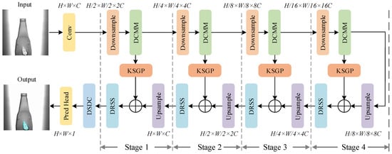
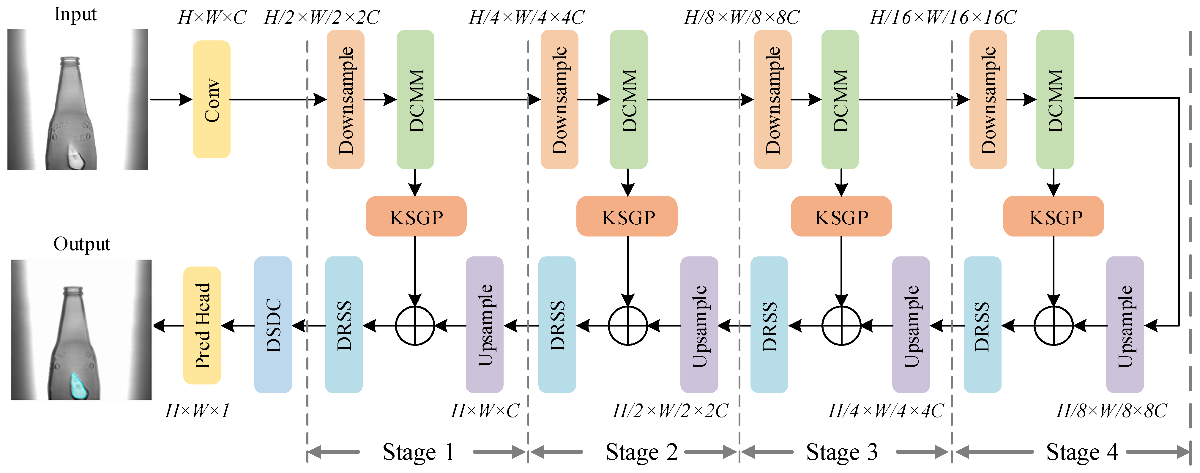
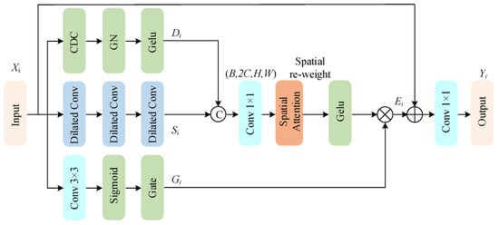
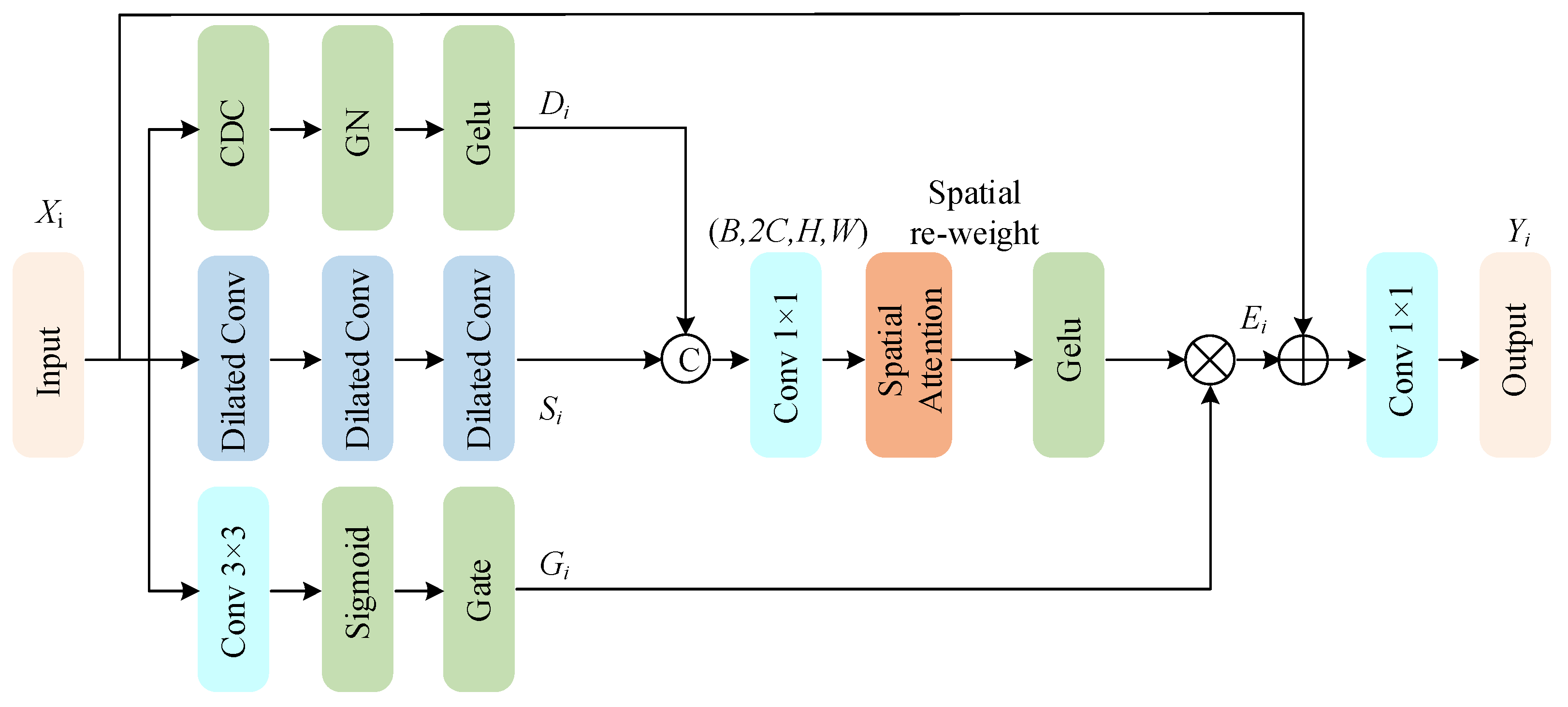
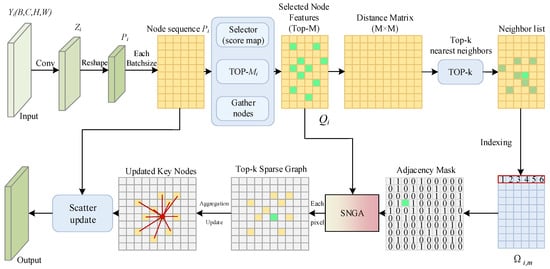
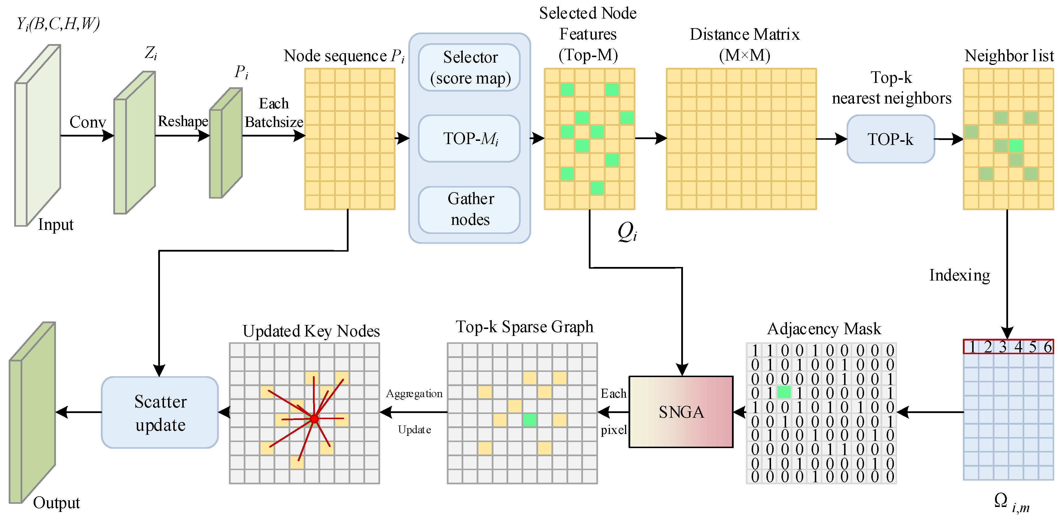
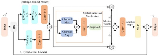
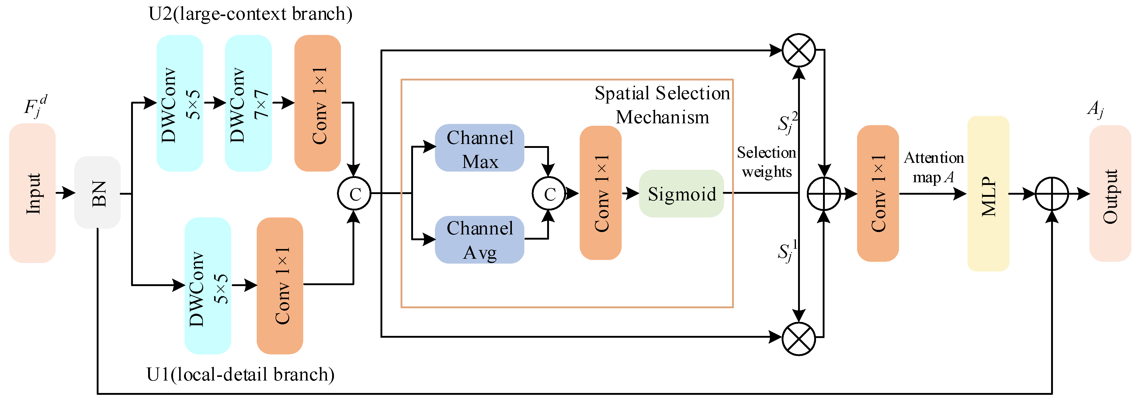
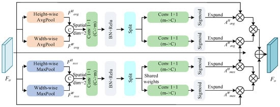
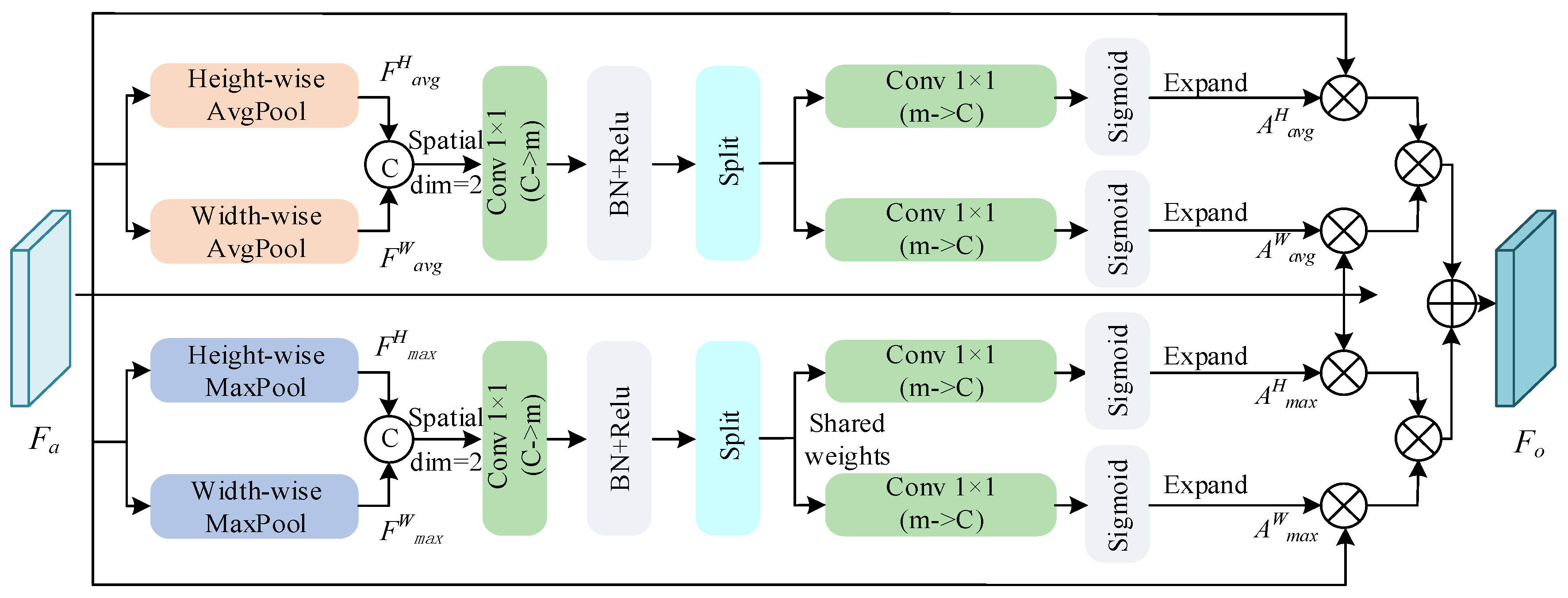
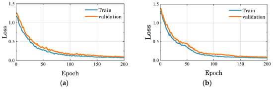
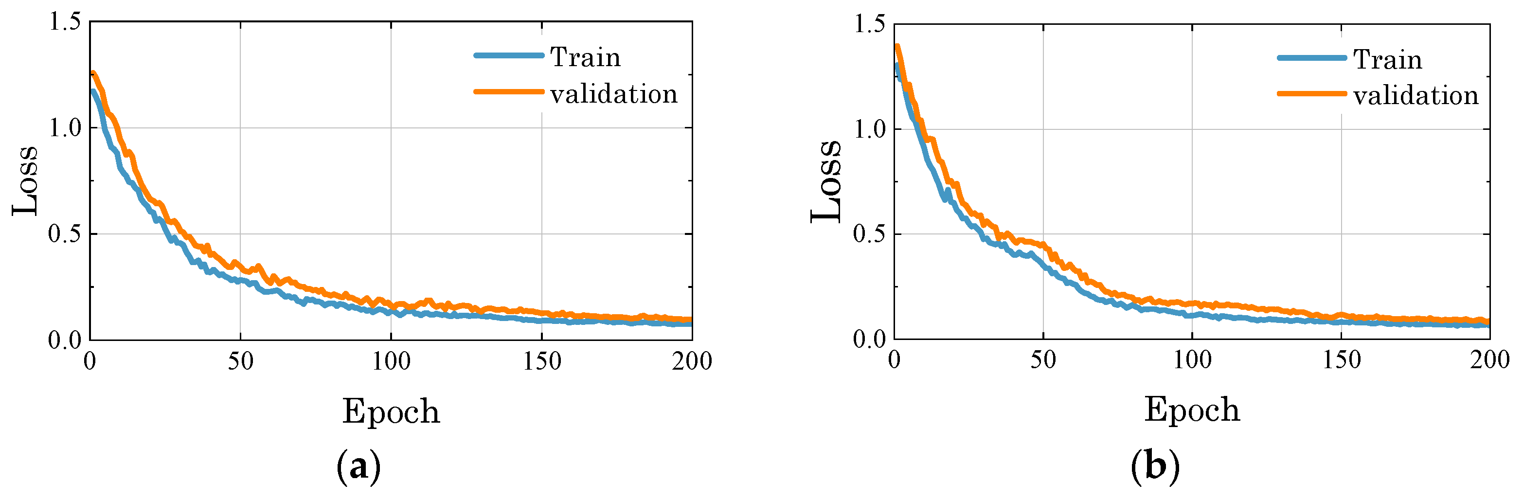
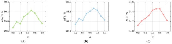
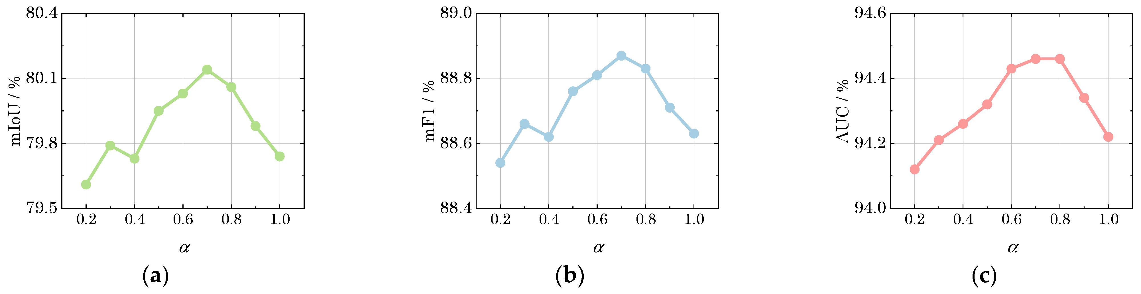
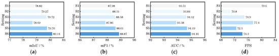
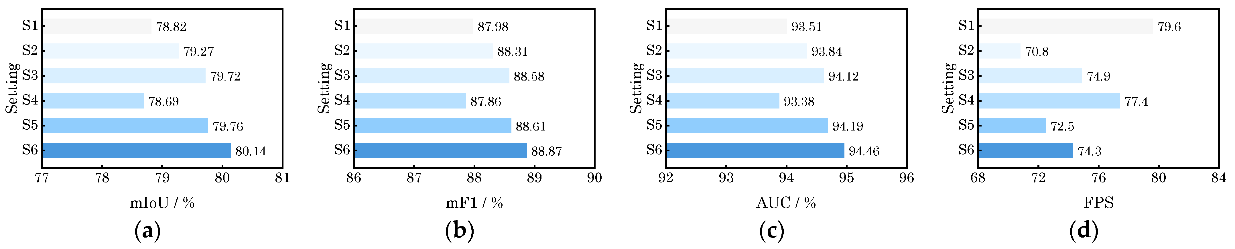
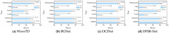
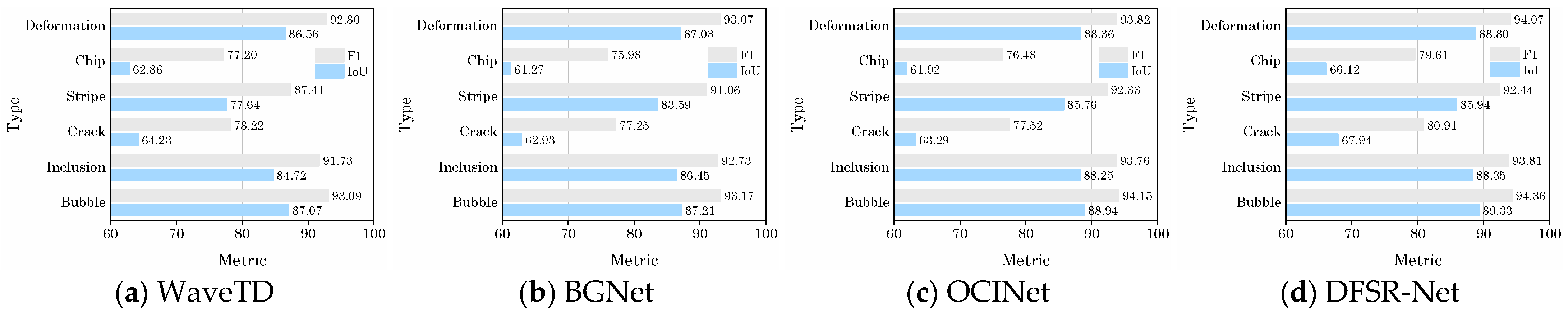
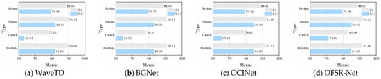
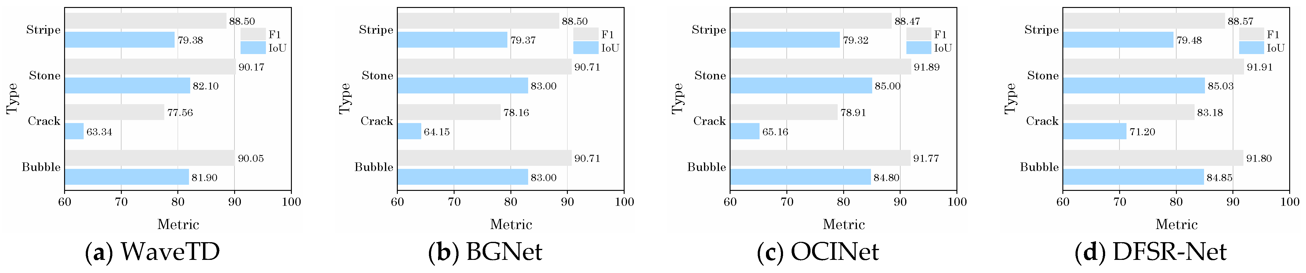
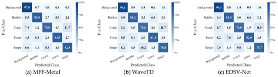
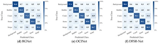
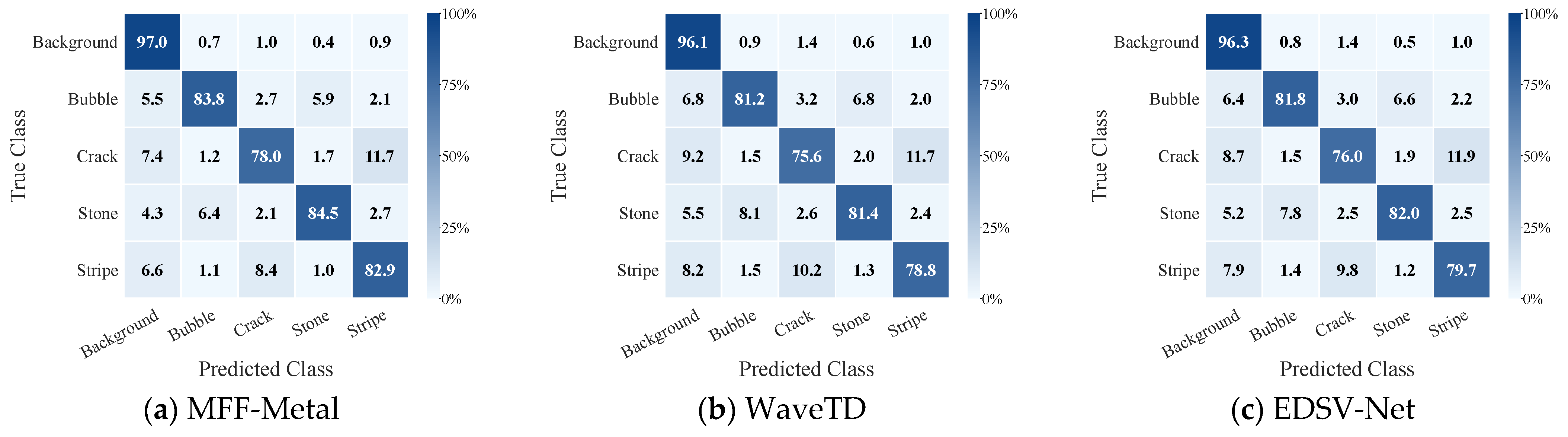
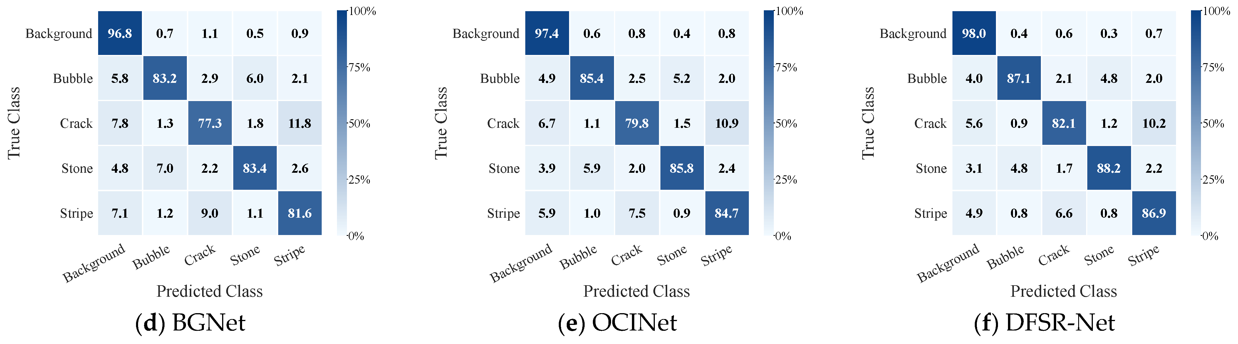
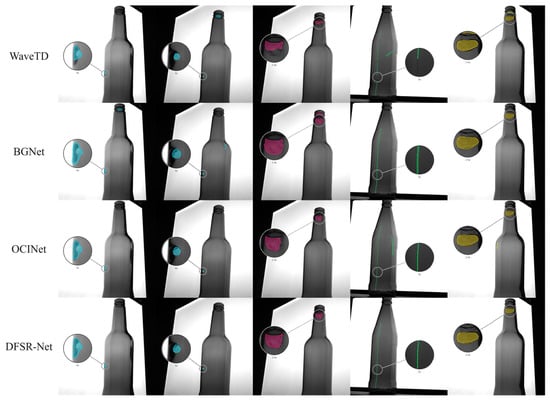
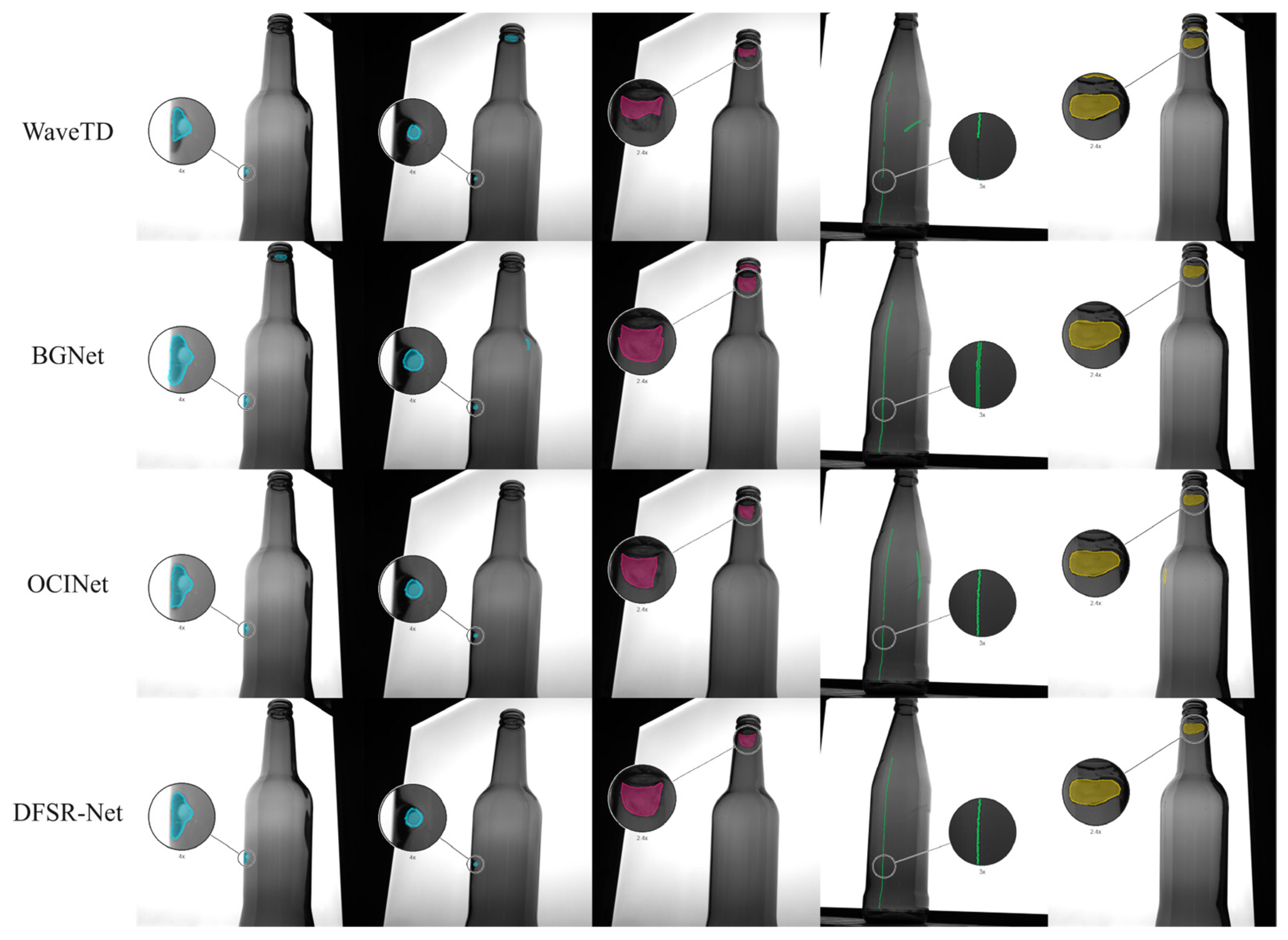
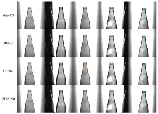
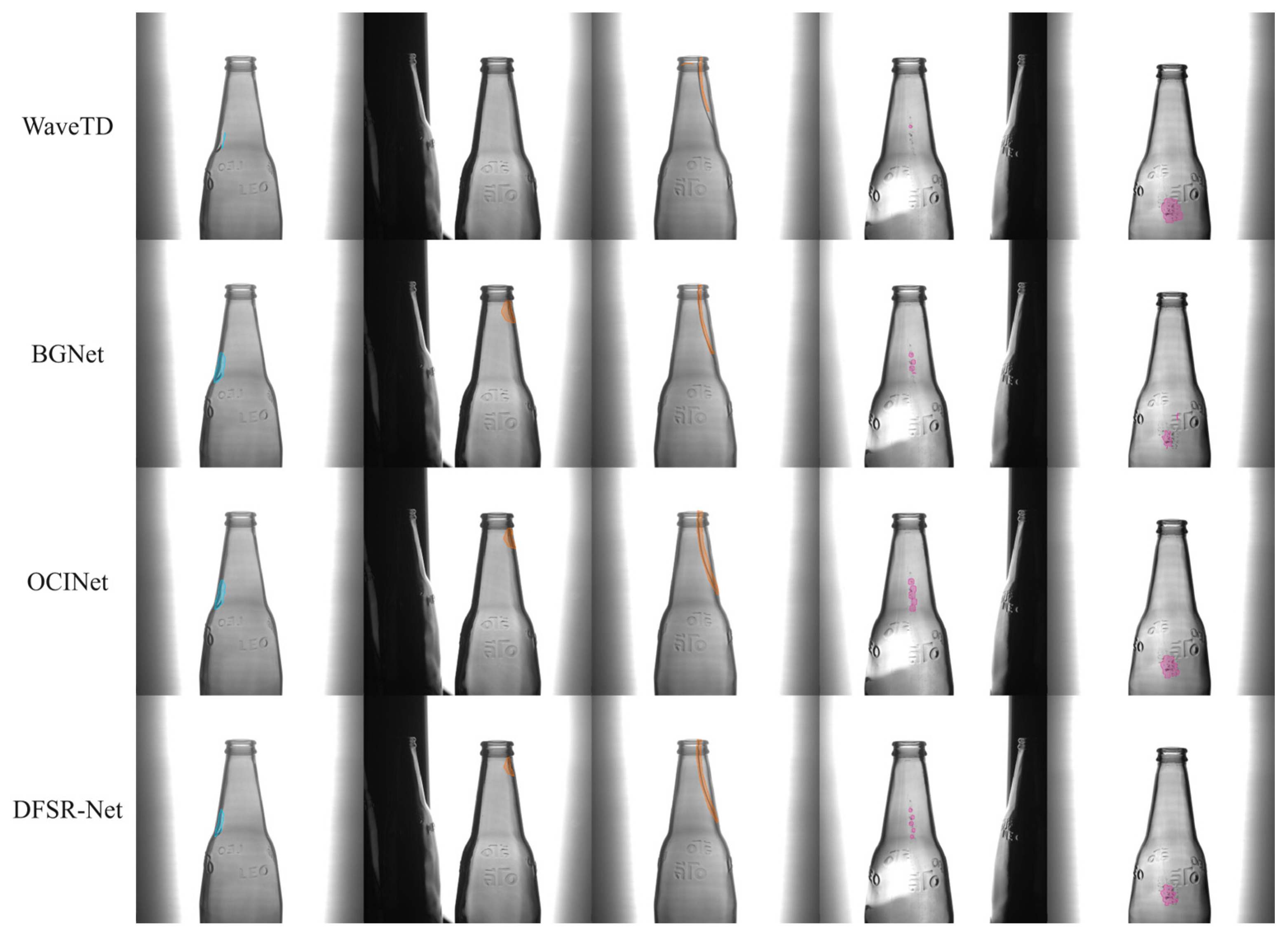
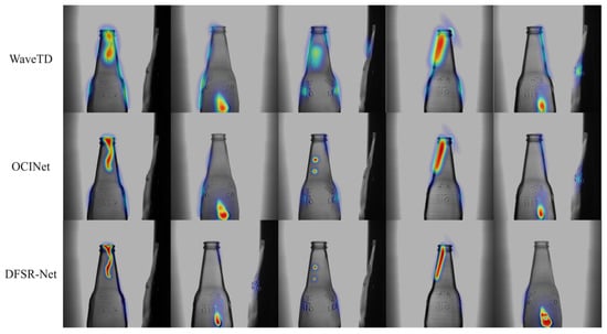
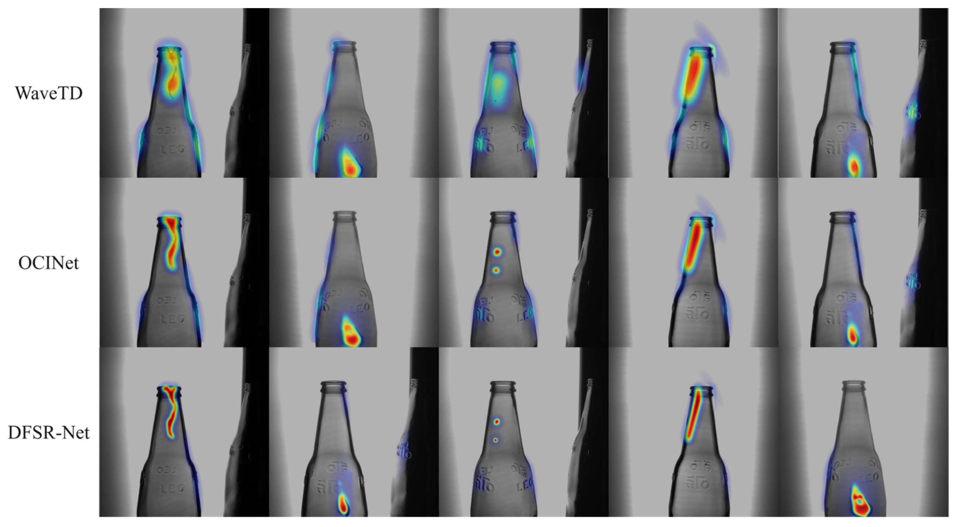



Disclaimer/Publisher’s Note: The statements, opinions and data contained in all publications are solely those of the individual author(s) and contributor(s) and not of MDPI and/or the editor(s). MDPI and/or the editor(s) disclaim responsibility for any injury to people or property resulting from any ideas, methods, instructions or products referred to in the content. |
© 2026 by the authors. Licensee MDPI, Basel, Switzerland. This article is an open access article distributed under the terms and conditions of the Creative Commons Attribution (CC BY) license.