


Abstract
Climate change has intensified hydrological extremes, placing complex stress on terrestrial ecosystems. Quantifying the decoupling between vegetation condition and water availability—termed vegetation–water asynchrony—is critical for sustainable ecosystem monitoring, yet no standardized remote sensing indicator exists. This study introduces the Asynchrony Index (AI) to quantify vegetation–water decoupling using Sentinel-2 data in northeastern Thailand. We analyzed 106 sampling points across four years (2019, 2020, 2023, 2024), calculating AI as the absolute difference between standardized NDVI and MNDWI. Four cross-validation strategies—GroupKFold, Leave-One-Year-Out, Spatially Blocked, and Random K-Fold—were employed to assess the predictive capability of five external environmental variables. Mixed-effects models accounted for repeated measures, and spatial autocorrelation was assessed using Moran’s I and LISA. AI exhibited significant interannual variation (ANOVA: F(3, 420) = 4.83, p = 0.0026), with the highest mean in 2020 (0.849) and the lowest in 2024 (0.547). No external predictor correlated strongly with AI (all |r| < 0.17), and PCA explained 70.9% of total variance in the first two components. Mixed-effects models revealed that 57.1% and 58.2% of variance was attributable to between-site differences (ICC = 0.571 and 0.582). Drought was not a significant predictor (p = 0.140). All models yielded negative R2 in GroupKFold (−0.61 to −0.09) and Spatial Block (−0.71 to −0.56), indicating insufficient predictive information. Residual Moran’s I remained significant (I = 0.252, p = 0.001), confirming that unmeasured factors drive asynchrony. Topographic clustering revealed three landscape units (F = 4.90, p = 0.0077), but effect sizes were small (η2 = 0.012). SHAP identified TWI, prox2river, and DEM as the most influential features. This study contributes an interpretable metric for ecosystem monitoring and demonstrates the importance of honest reporting of model limitations.
1. Introduction
1.1. Background and Sustainability Context
Climate change has intensified the frequency and severity of hydrological extremes across many parts of the world. Floods and droughts are becoming more frequent, longer-lasting, and more intense [1,2]. These shifts create difficult conditions for terrestrial ecosystems, as periods of water excess and water deficit disrupt the balance between what plants need and what the environment provides [3,4]. Understanding how ecosystems respond to such perturbations matters for developing monitoring and management strategies, particularly in regions that face both flood and drought events [5,6]. This understanding also sits at the heart of global sustainability efforts, because healthy ecosystems underpin food security, water availability, climate regulation, and human well-being [7]. The United Nations Sustainable Development Goals (SDGs) offer a framework for tackling these interconnected challenges [8]. SDG 6 (Clean Water and Sanitation) emphasizes monitoring water-related ecosystems, SDG 13 (Climate Action) calls for building resilience to climate-induced disasters [1], and SDG 15 (Life on Land) focuses on protecting terrestrial ecosystems and combating land degradation [8]. These goals are deeply intertwined and point to the need for integrated approaches to ecosystem monitoring that account for how vegetation and water resources interact under changing climatic conditions [9,10].
Remote sensing and GIS technologies have become essential tools in sustainability science, enabling systematic observation of environmental resources across multiple spatial and temporal scales [11,12]. The European Space Agency’s Sentinel-2 mission, with its high spatial resolution (10–20 m) and frequent revisit cycle (5 days), has made it possible to detect subtle changes in vegetation and water conditions that matter for sustainability assessment [13]. Vegetation indices such as the Normalized Difference Vegetation Index (NDVI) and water indices such as the Modified Normalized Difference Water Index (MNDWI) have been widely used to monitor vegetation health and surface water conditions, respectively [14,15]. In most studies, however, these indices are analyzed separately, which limits our ability to understand how vegetation and water resources interact [16]. The concept of vegetation–water synchrony—the degree to which vegetation condition and water availability change in concert—remains underexplored in sustainability research [17]. While individual indices provide valuable information, they do not capture the emergent properties that arise from vegetation–water interactions [18]. These interactions are particularly important in flood–drought-prone landscapes, where rapid transitions between hydrological extremes may create conditions of asynchrony [19,20].
Deep learning and ensemble methods have shown promise for large datasets, but their performance on datasets with fewer than 1000 observations remains uncertain, particularly when predictor–response relationships are weak [21]. This study therefore focuses on moderate-sized datasets and explores whether complex models can compensate for weak predictor–response relationships.
The upper Chi River Basin in northeastern Thailand offers a clear example of the sustainability challenges facing many agricultural regions in Southeast Asia. The region experiences alternating flood and drought events that threaten food security, livelihoods, and ecosystem services [22,23]. Recent studies in this region have demonstrated the utility of machine learning for drought characterization [22], flood risk assessment [23], drought vulnerability mapping [24], as well as spatial asymmetry in topographic controls on flood intensity [25]. However, the specific dynamics of vegetation–water coupling during flood–drought transitions remain unexplored in this region.
1.2. Research Gaps and Objectives
Despite growing data availability and analytical tools, several critical research gaps remain. First, there is no established sustainability indicator for quantifying vegetation–water decoupling using remote sensing data [26]. Existing indicators focus on either vegetation condition (e.g., NDVI) or water availability (e.g., MNDWI), but none integrate both dimensions into a single metric that captures their temporal decoupling. Second, the drivers of vegetation–water asynchrony remain poorly understood [27]. While drought severity is often assumed to be the primary driver of ecosystem stress, recent evidence suggests that local factors such as topography, soil properties, and groundwater dynamics may mediate ecosystem responses [28]. Third, the temporal dynamics of vegetation–water synchrony following disturbance events are not well-characterized [29]. Most studies rely on short time series (1–3 years), which cannot capture the multi-year recovery trajectories that are critical for understanding ecosystem resilience. Fourth, the applicability of machine learning approaches for moderate-sized sustainability datasets has not been fully explored [21]. Fifth, the spatial patterns of asynchrony and their relationship to landscape heterogeneity have not been adequately characterized [28].
To address these gaps, this study was designed with five objectives:
Develop an Asynchrony Index (AI) quantifying decoupling between NDVI and MNDWI using Sentinel-2 data [13,16], with both year-wise and common-reference standardization approaches.
Characterize temporal patterns of asynchrony across four years (2019, 2020, 2023, 2024), including flood (2019), drought (2020, 2024), and post-drought (2023) periods [29], using mixed-effects models to account for repeated measures.
Investigate relationships between AI and environmental variables using correlation analysis, four cross-validation strategies (GroupKFold, LOYO, Spatial Block, Random K-Fold), and SHAP analysis [21], with external predictors only to avoid circularity.
Examine spatial patterns of asynchrony through topographic clustering (K-means on DEM, TWI, Slope), global spatial autocorrelation (Moran’s I), local spatial autocorrelation (LISA), and residual spatial autocorrelation after regression on external predictors [28].
Provide methodological insights for applying machine learning to moderate-sized datasets in sustainability research [22,23,30], including honest reporting of model limitations when predictive performance is poor.
1.3. Research Questions and Hypotheses
Five research questions guided this study:
RQ1: Does AI vary significantly across years in response to hydrological perturbations?
RQ2: What are the relationships between AI and environmental variables?
RQ3: Can machine learning approaches predict AI using external predictors, and what does predictive performance reveal about data limitations?
RQ4: Is asynchrony primarily topographically determined or a complex emergent property?
RQ5: What are the implications for sustainable ecosystem monitoring in flood–drought-prone landscapes?
Based on these questions, five hypotheses were tested:
H1.
AI will vary significantly across years (ANOVA: p < 0.05 with higher asynchrony during drought (2020) and lower during post-drought (2024) periods [29].
H2.
AI will show weak correlations with individual environmental variables (|r| < 0.3), indicating emergent properties [18].
H3.
Predictive modeling using external variables will yield negative R2 values in spatially and temporally blocked cross-validation, indicating insufficient predictive information [30].
H4.
Asynchrony will not be primarily determined by topography alone (ANOVA: p > 0.05 for cluster differences) [28].
H5.
AI will provide complementary information to individual indices, supporting multi-indicator monitoring systems.
1.4. Significance and Novel Contributions
This study makes several novel contributions to sustainability science, remote sensing, and ecological modeling.
First, we introduce the Asynchrony Index (AI) as a simple, interpretable metric for quantifying vegetation–water decoupling. Unlike existing indicators that focus on either vegetation or water separately, AI integrates both dimensions into a single metric that captures emergent ecosystem properties. This metric can be calculated from freely available Sentinel-2 data, enabling operational monitoring across large regions.
Second, we demonstrate the importance of honest reporting of model limitations. While there is increasing pressure to apply sophisticated machine learning methods to ecological datasets, our results demonstrate that complex models cannot compensate for weak predictor–response relationships. The negative R2 values obtained in this study are not a failure but rather a valuable contribution to sustainability science, as they provide crucial information about data limitations and the boundaries of predictive capability [30].
Third, we provide methodological insights for moderate-sized datasets (n = 424 observations). By comparing four cross-validation strategies, we show that GroupKFold (with site as group) and Spatially Blocked CV provide more realistic assessments of model generalizability than random K-Fold, which can produce artificially inflated R2 values due to data leakage.
Fourth, we integrate remote sensing, GIS, and spatial analysis into a comprehensive framework for ecosystem monitoring. The combination of topographic clustering, Moran’s I, LISA, and residual spatial autocorrelation provides a multi-faceted view of vegetation–water dynamics that goes beyond simple index-based monitoring.
Fifth, we contextualize our findings within the SDG framework, demonstrating how remote sensing-based indicators can contribute to tracking progress toward SDG 6.6 (water-related ecosystems), SDG 13.1 (climate resilience), and SDG 15.3 (land degradation). This integration enhances the policy relevance of the research and provides a template for operationalizing sustainability monitoring [8,9].
2. Materials and Methods
2.1. Study Area and Data Collection
The upper Chi River Basin in northeastern Thailand served as the study area, encompassing three districts of Mahasarakham Province: Kosum Phisai, Kantharawichai, and Chiang Yuen (Figure 1a). This region represents the sustainability challenges common to agricultural areas across Southeast Asia, where shifting climate patterns intensify both flooding and drought, putting pressure on food production, local livelihoods, and ecosystem services [22,23]. Similar pressures affect monsoon-dependent farming regions worldwide, making this area a useful case for developing monitoring approaches that can inform climate adaptation and resource management.
Figure 1.
(a) Study area. (a) Distribution of 106 sampling points with drought severity levels (0–18) for 2019, 2020, 2023, and 2024, overlaid with historical flood inundation areas of 2018, 2021, and 2022 across the three districts. (b) Location of Mahasarakham Province in northeastern Thailand (inset), showing the three study districts Kosum Phisai, Kantharawichai, and Chiang Yuen within the upper Chi River Basin. Source: Adapted from Figure 1 of the original manuscript (unchanged). Basemap sources: Esri World Imagery (esri.com) and OpenStreetMap contributors (openstreetmap.org). GIS analysis and map production by the authors.
The study area lies within the Chi River floodplain, a major tributary of the Mun River system. Elevations range from 138–159 m above sea level, with predominantly flat to gently undulating terrain (slope < 1.2%). The climate is tropical savanna (Köppen: Aw), with annual precipitation of roughly 1200–1400 mm, most of which falls during the southwest monsoon from May to October. Mean annual temperature is 27.5 °C. Agricultural land dominates the landscape, primarily rice paddies and cassava plantations, with scattered fragments of dry deciduous forest and village settlements. Soils consist mainly of sandy loam and clay loam derived from alluvial and colluvial deposits, which shape local hydrological dynamics and farming practices. The study area covers approximately 1450 km2 of the lower Chi River floodplain, where seasonal flooding and drought occur regularly.
A total of 106 sampling points were distributed across the study area to capture the range of topographic, hydrological, and vegetation conditions present (Figure 1b). These points were selected based on farmer-reported drought occurrence within a 3.6 km radius from village centers, representing the average distance of agricultural plots affected by drought during the study period.
Drought and flood data came from a pre-existing, de-identified secondary dataset originally compiled for a related study in the same region [23]. The dataset contains village-level drought reports on a 0–18 scale, where higher values indicate more severe drought. These reports are based on agricultural impact assessments conducted by local authorities under the Department of Disaster Prevention and Mitigation (DDPM), Thailand. Drought data were compiled for 2019, 2020, 2023, and 2024. Flood intensity data were compiled for 2018, 2021, and 2022. The year-by-variable availability of all environmental data is summarized in Table S1 (Supplementary Materials).
Sampling points were georeferenced and kept consistent across all observation years to enable temporal analysis.
2.2. Satellite Data and Spectral Indices
Sentinel-2 imagery (Level-2A, atmospherically corrected surface reflectance) was acquired for four years (2019, 2020, 2023, 2024) during the dry season (March–May) to reduce seasonal variability. Images with less than 10% cloud cover were selected, and all data were resampled to 10 m spatial resolution [13]. The B11 band was resampled using bilinear interpolation. Sentinel-2 data are freely available, which supports reproducible monitoring and aligns with open science principles.
Four spectral indices were calculated from Sentinel-2 bands (Table 1). Each index was chosen for its established relevance to vegetation and water dynamics.
Table 1.
Spectral indices calculated from Sentinel-2 data.
NSMI (Normalized Soil Moisture Index) was excluded because it is algebraically redundant with NDMI, as confirmed by a near-perfect negative correlation (r = −1.00) in preliminary checks [18]. The VCI reference range was defined using the minimum and maximum NDVI values observed across the entire study period (2018–2024) for each sampling point.
2.3. Topographic and Environmental Variables
Topographic variables were derived from a 30 m Digital Elevation Model (DEM) (Table 2). These variables are fundamental to understanding hydrological connectivity and ecosystem functioning [28], and they help identify areas vulnerable to vegetation–water decoupling.
Table 2.
Topographic and environmental variables.
Drought severity was recorded for 2019, 2020, 2023, and 2024 on a 0–18 scale, with higher values indicating more severe drought. This scale was applied consistently across all four years. Flood intensity was recorded for 2018, 2021, and 2022 but is not included in the final analysis because the four-year dataset (2019, 2020, 2023, 2024) does not overlap with the flood years.
2.4. Asynchrony Index (AI) Calculation
The Asynchrony Index (AI) was calculated as the absolute difference between standardized NDVI and MNDWI values (Equations (1)–(3)). This indicator quantifies decoupling between vegetation condition and surface water availability, providing an integrated measure of potential ecosystem stress [16,18].
AI = ∣Z(NDVI) − Z(MNDWI)∣
Z(NDVI) = (NDVI − μNDVI)/σNDVI
Z(MNDWI) = (MNDWI − μMNDWI)/σMNDWI
Here μ and σ represent the mean and standard deviation for each index.
Two standardization approaches were used:
Year-wise standardization (primary approach): Each year’s NDVI and MNDWI values were standardized separately using that year’s mean and standard deviation. This ensures that AI values reflect the relative position of each observation within its respective year, accounting for interannual differences in the magnitude and variability of spectral indices [16]. However, this approach removes interannual differences in means and variances, so AI values should be interpreted as changes in relative synchrony within each year rather than absolute measures of ecosystem recovery.
Common reference standardization (supplementary approach): NDVI and MNDWI values were pooled across all four years and standardized using a common mean and standard deviation. This preserves interannual differences and enables cross-year comparisons of absolute synchrony. Results from this approach appear in Supplementary S2 (see Figure S1 and Table S2).
AI values range from 0 (perfect synchrony) to higher values (greater asynchrony). Higher AI indicates greater decoupling between vegetation condition and surface water availability, suggesting potential ecosystem stress. An alternative Asynchrony_NDMI was also calculated (Equation (4)) to explore whether vegetation moisture content (NDMI) provides a different perspective compared to surface water (MNDWI) [16]:
AI_NDMI = ∣Z(NDVI) − Z(NDMI)∣
2.5. Data Preparation
Data processing was carried out in Python (version 3.10) using pandas (1.5.0) for data manipulation, numpy (1.23.0) for numerical operations, scikit-learn (1.1.0) for machine learning, xgboost (1.7.0) for XGBoost, shap (0.41.0) for model interpretation, and matplotlib (3.6.0) and seaborn (0.12.0) for visualization. Using open-source Python libraries supports reproducibility and accessibility.
- Data cleaning steps:
Removed NSMI due to algebraic redundancy with NDMI (r = −1.00) [18].
Removed 9 sampling points (FID 31, 34, 35, 41, 137, 138, 149, 166, 174) where prox2river could not be reliably determined (values of 0 m, likely a data artifact).
Checked for missing values (none detected in the final dataset).
- Final dataset:
4-year dataset: 106 points × 4 years (2019, 2020, 2023, 2024) = 424 observations
The 4-year dataset was used for all analyses, including temporal trend analysis, mixed-effects models, correlation analysis, PCA, predictive modeling, and spatial autocorrelation. A year-by-variable availability table is provided in Table S1 (Supplementary Materials).
2.5.1. Descriptive Statistics
Descriptive statistics (mean, standard deviation, minimum, maximum, quartiles) were calculated for all environmental variables overall and by year. The coefficient of variation was calculated to assess heterogeneity in AI across the study area.
2.5.2. Analysis of Variance (ANOVA) and Effect Sizes
One-way ANOVA tested for significant differences in AI across years. Effect sizes were calculated to quantify the magnitude of differences. Eta-squared (η2) represents the proportion of variance in AI explained by year [31]. Cohen’s d represents the standardized mean difference between year pairs [32]. 95% confidence intervals were calculated for mean AI values. Post hoc comparisons used Tukey’s Honest Significant Difference (HSD) test to identify which year pairs differed significantly.
Given the right-skewed distribution of AI, we verified ANOVA assumptions including normality of residuals (Shapiro–Wilk test) and homogeneity of variance (Levene’s test). Where assumptions were violated, we applied log transformation and confirmed that results were qualitatively unchanged.
2.5.3. Mixed-Effects Models
To account for repeated measures across years at the same sampling points, mixed-effects models were fitted:
Model 1 (4 years): AI ~ Year + (1|FID)
Model 2 (4 years with drought): AI ~ Year + Drought + (1|FID)
The Intraclass Correlation Coefficient (ICC) quantified the proportion of variance attributable to between-site differences. ICC values were interpreted as follows: ICC < 0.20 (low clustering), 0.20–0.50 (moderate clustering), ICC > 0.50 (high clustering). These models address pseudoreplication concerns, as the same 106 locations were measured repeatedly across years, violating the independence assumption of standard ANOVA [31].
Model fitting used the statsmodels library in Python with restricted maximum likelihood (REML) estimation. Model comparison used likelihood ratio tests and Akaike Information Criterion (AIC).
2.5.4. Correlation Analysis
Pearson correlation coefficients were calculated among all environmental variables to identify collinearity and relationships. The correlation matrix was visualized using a heatmap. Correlation coefficients with AI were calculated for all external predictors, with significance assessed at p < 0.05 and p < 0.01 levels.
2.5.5. Principal Component Analysis (PCA)
PCA was performed to reduce dimensionality and identify the underlying environmental gradients structuring the dataset. The analysis included seven variables: four spectral indices (NDVI, MNDWI, NDMI, VCI) and three topographic variables (DEM, TWI, Slope). All variables were standardized to zero mean and unit variance before PCA to ensure that variables with different units contributed equally to the analysis.
The analysis was conducted on the full 4-year dataset (n = 424 observations). The number of components was set to two, which allowed visualization of the dominant gradients in a two-dimensional space. The explained variance ratio for each component was calculated, and the loadings were interpreted to identify the contribution of each variable to the principal components. Sample projections on the PC1–PC2 plane were colored by AI values to visualize whether sampling points with high asynchrony cluster in specific regions of the environmental space. Bartlett’s test of sphericity confirmed that the correlation matrix was suitable for PCA (χ2 = 1939.67, df = 21, p < 0.001).
The purpose of the PCA in this study was not to reduce the predictor set for downstream modeling (which retained all five external predictors) but to characterize the structure of the environmental gradients and to assess whether asynchrony is associated with particular combinations of moisture and topographic conditions. A key diagnostic was whether sampling points with high AI values cluster in a specific region of the PCA space or are distributed across the full range of environmental conditions.
2.6. Analytical Approach: From Prediction to Explanation
Given the exploratory nature of this study and the moderate sample size (n = 424), we adopted a hierarchical analytical approach that prioritizes honest assessment of data capabilities and limitations [32].
2.6.1. Primary Analysis: Correlation and Statistical Inference
Our primary analytical framework focused on characterizing temporal and spatial patterns of AI using descriptive statistics with 95% confidence intervals, ANOVA with effect sizes, Tukey HSD post hoc tests, Pearson correlation analysis, PCA, and K-means clustering. This approach provides an honest assessment of relationships present in the data without over-extrapolating or imposing complex models on weak relationships. By prioritizing interpretability and transparency, this framework supports evidence-based sustainability decision-making [9].
2.6.2. Supplementary Analysis: Predictive Modeling
To explore whether complex non-linear relationships could improve prediction, we applied multiple machine learning algorithms with four cross-validation strategies.
Data Splitting and Cross-Validation: Four cross-validation strategies were employed to assess model generalizability under different assumptions:
GroupKFold (5-fold): FID as group identifier. This prevents pseudoreplication by ensuring that the same sampling point (FID) does not appear in both training and test sets across different years. Each fold maintained a test size of approximately 20% of observations (85 samples for the 4-year dataset).
Leave-One-Year-Out (LOYO): Each year serves as the test set once, with all other years used for training. This tests temporal generalization—can the model predict a completely unseen year?
Spatially Blocked Cross-Validation: Sampling points are divided into spatial blocks using K-means clustering on coordinates, with entire blocks held out for testing. This tests spatial generalization—can the model predict a new area?
Random K-Fold (5-fold): Standard random splitting. This serves as a baseline but may produce artificially inflated R2 values due to data leakage (same FID in train and test sets).
Comparing these strategies provides critical insights into model generalizability [32].
Standardization: All features were standardized using StandardScaler (zero mean, unit variance) fitted on training-fold data only to prevent data leakage.
Predictor Selection: To avoid circularity, NDVI and MNDWI were excluded from the predictor set. Only external variables were used: topographic (DEM, TWI, Slope), hydrological (prox2river), and disturbance (Drought severity, 0–18 scale).
Models Tested:
Linear Regression (baseline);
Random Forest (ensemble of decision trees);
XGBoost (gradient boosting).
Model Evaluation: Performance was evaluated using R2, RMSE, and MAE. Negative R2 values indicate that the model performed worse than predicting the mean, which provides important information about the limitations of the data and predictors [32]. This interpretation is stated explicitly to ensure transparent reporting.
Alternative Formulations Tested: Recognizing the potential limitations of the predictor set, we tested additional formulations: (1) adding NDMI and VCI as predictors (acknowledging partial circularity), (2) using AI_NDMI as the response variable, and (3) Linear Regression as a simpler baseline for comparison.
2.6.3. Deep Learning Models
For completeness, we tested LSTM, CNN, and Hybrid (CNN + LSTM) architectures. Due to the limited sample size (n = 424), these models were expected to perform poorly, as deep learning models generally require thousands to millions of samples to achieve optimal performance [21]. These results are reported in Supplementary S1. We emphasize that these results are dataset-specific and do not constitute a general claim about the suitability of deep learning for ecological datasets.
2.7. Feature Importance and Model Interpretation
2.7.1. Model-Based Feature Importance
Feature importance was calculated to identify potential drivers of asynchrony and inform targeted monitoring and management. For Linear Regression, importance was calculated as the absolute value of standardized coefficients. For Random Forest and XGBoost, importance was calculated as the mean decrease in impurity (MDI) across all trees. Due to the negative R2 values obtained in spatially and temporally blocked cross-validation, feature importance results are interpreted with caution and supplemented by correlation analysis.
2.7.2. SHAP Analysis Procedure
SHAP (SHapley Additive exPlanations) analysis was conducted to interpret model predictions at the individual sample level, identify feature contributions to predictions, and visualize relationships between features and predicted outcomes. SHAP values were calculated for all 424 observations (4-year dataset) using both Random Forest and XGBoost models. Global importance was computed as the mean absolute SHAP value across all samples. Dependence plots were generated to visualize the relationship between feature values and SHAP values. Waterfall plots were generated for extreme cases (highest and lowest AI values). SHAP interaction values were computed for 200 randomly sampled observations to identify potential interaction effects.
Due to negative R2 values in GroupKFold and SpatialBlock cross-validation, SHAP patterns do not reflect true ecological drivers. SHAP importance indicates which variables the model used, not which variables cause asynchrony. These results should be treated as exploratory, not confirmatory, and should not be used as management targets without independent validation [32].
2.8. Spatial Clustering and Spatial Autocorrelation Analysis
2.8.1. K-Means Clustering
K-means clustering was performed on topographic variables (DEM, TWI, Slope) to identify distinct landscape units [28]. The elbow method was used to determine the optimal number of clusters (k), evaluating inertia values for k = 2 to 7. The optimal k was determined at k = 3, where the rate of decrease in inertia begins to diminish.
2.8.2. Cluster Characterization
Clusters were characterized by their mean values of topographic variables (DEM, TWI, Slope) and AI. ANOVA tested for significant differences among clusters, assessing whether topography alone determines asynchrony patterns. Tukey HSD post hoc tests identified which cluster pairs differed significantly. Effect sizes (Cohen’s d) were calculated for pairwise comparisons.
2.8.3. Global and Local Spatial Autocorrelation
Global spatial autocorrelation was assessed using Moran’s I for each year (2019, 2020, 2023, 2024). Moran’s I values range from −1 (perfect dispersion) to +1 (perfect clustering), with 0 indicating random spatial pattern. Statistical significance was assessed using 999 permutations. Spatial weights were defined using Queen contiguity with row standardization. Local spatial autocorrelation was assessed using Local Indicators of Spatial Association (LISA) to identify significant spatial clusters (High–High, Low–Low) and spatial outliers (High–Low, Low–High). The number and percentage of significant LISA clusters were recorded for each year. Multiple testing was addressed using the Benjamini–Hochberg false discovery rate (FDR) correction at α = 0.05.
2.8.4. Residual Spatial Autocorrelation Analysis
To assess whether the predictor set captures all spatial structure in AI, we calculated Moran’s I on the residuals from a linear regression of AI on all external predictors. Residuals were aggregated to site level (mean AI per FID) to avoid pseudoreplication. Significant residual spatial autocorrelation indicates that unmeasured factors drive spatial patterns in asynchrony, supporting the conclusion that asynchrony is a complex emergent property [28].
2.9. Reproducibility and Open Science
All analyses are fully reproducible. The complete dataset, analysis scripts, and documentation are available in the Zenodo repository: Littidej, P. (2026). Supplement and Materials [Dataset]. Zenodo. https://doi.org/10.5281/zenodo.23365879.
The repository contains: (1) original dataset (data4drought_flood_edit.xlsx), (2) processed dataset (dataset_final_4year.csv), (3) dataset with cluster assignments (dataset_final_4year_with_clusters.csv), (4) full reproduction script (analysis_reproduction.py), (5) README documentation, (6) requirements.txt, and (7) LICENSE (CC BY 4.0).
Random seeds were set to 42 for all stochastic operations. Open-source Python libraries (pandas, numpy, scikit-learn, xgboost, shap, libpysal, esda) support reproducibility and accessibility.
2.10. Integration with Sustainability Assessment Frameworks
To enhance the policy relevance of our findings, the Asynchrony Index (AI) was linked to three Sustainable Development Goal (SDG) targets [8,9,10]. SDG 6.6 (water-related ecosystems) was selected because AI integrates surface water availability (MNDWI) with vegetation condition (NDVI), supporting indicator 6.6.1 on changes in water-related ecosystems over time [33]. SDG 13.1 (climate resilience) was selected because AI responds to hydrological extremes and can serve as an indicator of ecosystem sensitivity to climate-induced stress [1]. SDG 15.3 (land degradation) was selected because vegetation–water decoupling is a potential early warning signal of land degradation in agricultural landscapes [8].
Sustainability Analysis Procedure
The sustainability integration step (Step 10 in Figure 2) followed three sequential procedures. First, AI values were linked to the three SDG targets described above, each documented with reference to its specific indicator (6.6.1, 13.1.1, and 15.3.1). Second, vulnerability mapping was performed by overlaying AI with topographic (DEM, TWI, Slope) and hydrological (prox2river) variables to identify locations where high asynchrony (AI > 0.95, the 75th percentile; see Table 3) coincides with unfavorable environmental conditions. Third, the resulting spatial patterns were translated into monitoring and policy recommendations, including the integration of AI into drought early warning systems and the prioritization of interventions in high-AI areas (Section 4.9).
Figure 2.
Analytical workflow. Flowchart summarizing the ten-step analytical procedure: (1) Data acquisition (Sentinel-2, SRTM DEM, DDPM records); (2) Preprocessing (cloud masking < 10%, resampling to 10 m, March–May dry-season composite); (3) Variable calculation (spectral indices: NDVI, MNDWI, NDMI, VCI; topographic variables: DEM, TWI, Slope, prox2river); (4) Asynchrony Index (AI) calculation with year-wise and common-reference standardization; (5) Statistical analysis (ANOVA, Tukey HSD, mixed-effects models, correlation); (6) PCA (eigenvalues, loadings, sample projection); (7) Predictive modeling (Linear Regression, Random Forest, XGBoost; four CV strategies); (8) SHAP analysis (global importance, dependence, waterfall, interaction); (9) Spatial analysis ((9a): K-means clustering; (9b): Moran’s I, LISA, residual autocorrelation); (10) Sustainability integration, in which AI patterns are linked to SDG 6.6 (water-related ecosystems), SDG 13.1 (climate resilience), and SDG 15.3 (land degradation) through vulnerability mapping that combines AI with topographic and hydrological variables, and translated into monitoring and policy recommendations (Section 2.10).
Table 3.
Descriptive statistics of environmental variables (4-year dataset, n = 424).
This step is qualitative and interpretive rather than inferential. No independent SDG indicator dataset was available for quantitative validation at the study scale, and the procedures are intended to provide a structured framework for linking AI to sustainability monitoring and policy, rather than to produce statistically validated sustainability metrics. Detailed spatial patterns and recommendations are presented in Section 3.12, Section 4.6 and Section 4.9.
3. Results
3.1. Descriptive Statistics
Table 3 summarizes the distribution of all environmental variables across the 4-year dataset (n = 424). The Asynchrony Index (AI) spanned a wide range, from 0.0002–3.909, with a mean of 0.706 and a standard deviation of 0.603. The coefficient of variation reached 85.3%, confirming that asynchrony varies considerably across the landscape. Some locations stayed nearly synchronized throughout the study period, while others drifted into extreme decoupling. The median value of 0.572 sat below the mean, a clear sign of right-skewness. Most sampling points experienced moderate asynchrony, but a small number of locations pulled the mean upward. For sustainability planning, this pattern argues against uniform, landscape-wide interventions and instead favors approaches tailored to specific hotspots.
MNDWI averaged −0.349 with a standard deviation of 0.108. The consistently negative values confirm that the study region is predominantly terrestrial rather than aquatic, which is expected because sampling points were placed on agricultural land. The interquartile range (IQR = 0.212) suggests that surface water conditions stayed relatively stable across most sampling points. NDVI averaged 0.260 ± 0.051, pointing to moderate vegetation cover with substantial spatial variation. The VCI range (0.276–0.643) shows that vegetation conditions spanned from stressed to healthy, reflecting the landscape’s heterogeneous response to hydrological variability.
Topographic variables showed moderate variability. TWI ranged from 9.516–12.824, and DEM from 138.699–158.781 m. The narrow elevation range of about 20 m indicates that the study area occupies a relatively homogeneous topographic setting, which limits the degree of topographic differentiation that can be captured. Slope values (0.440–1.049%) confirm that the terrain is predominantly flat to gently undulating. Drought severity averaged 2.755 ± 2.335, ranging from 0–18.
3.2. Temporal Patterns: Changes in Relative Synchrony
Figure 3 presents the interannual distribution of AI values across the four study years. The boxplot reveals how the spread and central tendency of AI shifted from 2019 to 2024.
Figure 3.
Boxplot showing the distribution of Asynchrony Index by year (2019–2024). The box represents the interquartile range (IQR), the line within the box indicates the median, and whiskers extend to 1.5 × IQR. Points beyond the whiskers represent outliers. Panel (a) shows the AI distribution by year; panel (b) shows the mean AI (±SD) by year. Source: Recalculated and regenerated from the 4-year dataset (424 records).
The AI exhibited significant interannual variation (ANOVA: F(3, 420) = 4.83, p = 0.0026). Table 4 presents the mean values of all environmental variables by year, showing that the highest AI mean occurred in 2020 (0.849 ± 0.729) and the lowest in 2024 (0.547 ± 0.490). This represents a 35.5% reduction in mean AI from 2020 to 2024. However, as noted in the methods Section 2.4, the year-wise standardization approach removes interannual differences in means and variances. These changes should therefore be interpreted as changes in relative synchrony within each year rather than absolute measures of ecosystem recovery.
Table 4.
Mean values of environmental variables by year (4-year dataset, n = 424).
Table 5 presents the effect sizes and 95% confidence intervals for mean AI values by year. The confidence intervals confirm that the highest AI values in 2020 (95% CI: 0.710–0.988) and 2019 (95% CI: 0.630–0.869) were higher than the lowest values in 2024 (95% CI: 0.454–0.640). The intervals for 2019 and 2023 (0.583–0.774) overlapped, consistent with the non-significant difference between these years.
Table 5.
Effect sizes and confidence intervals for Asynchrony Index by year (n = 424).
Eta-squared (η2) = 0.033 (small effect size, indicating that year explains approximately 3.3% of the variance in AI).
Table 6 presents the Tukey HSD post hoc test results for pairwise year comparisons. Significant differences were found between 2020 and 2024 (p = 0.0014). The 2019 vs. 2024 comparison was marginally non-significant (p = 0.0645). The largest differences were between 2020 and 2024 (mean difference = 0.302) and between 2019 and 2024 (mean difference = 0.203). The non-significant difference between 2019 and 2020 (p = 0.617) indicates that these two years had similar levels of relative synchrony.
Table 6.
Tukey HSD post hoc test results (n = 424).
Cohen’s d effect sizes: 2020 vs. 2024: d = 0.486 (medium effect); 2019 vs. 2024: d = 0.360 (small–medium effect).
The boxplot for 2020 revealed a bimodal distribution, with one cluster of points exhibiting asynchrony values below 0.5 and another cluster exceeding 1.0. This pattern points to two distinct response regimes: some locations maintained synchrony between vegetation and water conditions despite drought, while others experienced severe decoupling. The presence of these divergent responses within the same year underscores the role of local factors in mediating ecosystem sensitivity to drought.
3.3. Correlation Analysis
Figure 4 presents the correlation matrix among AI and the five external predictors used in this study.
Figure 4.
Correlation matrix of Asynchrony Index (AI) and external predictors (n = 424). Red indicates positive correlation, blue indicates negative correlation. Only the lower triangle is shown for clarity. Variables include DEM (elevation), TWI (Topographic Wetness Index), Slope, prox2river (distance to river), and Drought. Source: Recalculated and regenerated from the 4-year dataset (424 records).
The strongest correlations in the matrix appear among the topographic variables themselves rather than between AI and any predictor. TWI and Slope showed a strong negative correlation (r = −0.64), which is expected because wetter areas tend to occupy flatter positions in the landscape. DEM and Slope were positively correlated (r = 0.33), indicating that higher elevations in this basin tend to have slightly steeper gradients. TWI and prox2river were negatively correlated (r = −0.61), reflecting the tendency for sites closer to the river to occupy flatter, wetter positions. These internal correlations among predictors are consistent with the known topography of the Chi River floodplain and confirm that the predictor set captures meaningful landscape structure.
Table 7 presents the correlation coefficients between AI and each external predictor. No predictor showed a correlation with AI stronger than |r| = 0.17. The highest correlation was with DEM (r = 0.162, p = 0.0008), followed by Slope (r = 0.130, p = 0.0076) and TWI (r = −0.112, p = 0.0214). The remaining predictors showed correlations below |r| = 0.09: prox2river (r = 0.084, p = 0.085) and Drought (r = 0.039, p = 0.425).
Table 7.
Correlation coefficients between Asynchrony Index (AI) and external predictors (n = 424). Source: Recalculated from the 4-year dataset (424 records).
Three predictors reached statistical significance: DEM (r = 0.162, p = 0.0008), Slope (r = 0.130, p = 0.0076), and TWI (r = −0.112, p = 0.0214). Even these significant correlations are weak in absolute terms—they explain less than 2.6% of the variance in AI individually (DEM: r2 = 0.026; Slope: r2 = 0.017; TWI: r2 = 0.013). The remaining two predictors—prox2river and Drought—showed no statistically significant relationship with AI at the 0.05 level.
The near-zero correlation between Drought and AI (r = 0.039, p = 0.425, n = 424) is particularly noteworthy. This finding indicates that drought severity, when measured independently of other environmental factors, does not determine vegetation–water decoupling in this landscape. A site experiencing severe drought may or may not exhibit high asynchrony, depending on local conditions that are not captured by drought intensity alone. This result is consistent with the mixed-effects model findings reported in Section 3.5, where drought was not a significant predictor of AI (p = 0.140).
Correlations between AI and spectral indices were also calculated for completeness: NDVI (r = 0.080, p = 0.100), MNDWI (r = −0.086, p = 0.078), NDMI (r = −0.018, p = 0.705), and VCI (r = 0.031, p = 0.520). None were statistically significant.
The weak correlations observed across all predictors carry two important implications for the study. First, they suggest that AI captures information that is not redundant with any single environmental variable. If AI were simply a proxy for, say, elevation or drought severity, we would expect a strong correlation with that variable. The absence of such a correlation supports the interpretation of AI as an emergent property reflecting the combined influence of multiple interacting factors. Second, the weak correlations provide an early indication of why predictive modeling may struggle: if no single predictor correlates strongly with AI, a model that combines them linearly is unlikely to achieve high predictive accuracy. This expectation is confirmed in Section 3.6, where all models yielded negative R2 values under GroupKFold and SpatialBlock cross-validation.
3.4. Principal Component Analysis
PCA was performed to reduce dimensionality and identify the underlying environmental gradients structuring the dataset. The analysis included seven variables: four spectral indices (NDVI, MNDWI, NDMI, VCI) and three topographic variables (DEM, TWI, Slope). Figure 5 presents the sample projection and loading vectors.
Figure 5.
PCA of environmental variables (n = 424). (a) Sample projection with colors representing Asynchrony Index (AI) values; (b) loading vectors illustrating the contribution of each environmental variable to the principal components. PC1 = 43.19%, PC2 = 27.67%, cumulative = 70.86%.
The first two principal components captured 70.86% of the total variance, with PC1 accounting for 43.19% and PC2 explaining 27.67%. This is a relatively high proportion of variance explained, which indicates that the seven variables are strongly correlated with each other and that the dataset is dominated by two underlying gradients. This result is consistent with the TWI–Slope correlation of r = −0.64, which implies that PC1 must explain at least 41.3% of the variance; our value of 43.19% confirms this expectation.
The loading vectors in Figure 5b reveal the structure of each component. PC1 was primarily defined by NDMI (0.53), VCI (0.53), NDVI (0.40), and MNDWI (0.39) on the positive side, with TWI (−0.23) on the negative side. This component represents a gradient that separates sites with high vegetation moisture and health from sites with lower values. In the context of AI, this is the most directly relevant component because it captures the variables that are combined to compute the index.
PC2 was primarily defined by TWI (0.55) and MNDWI (0.35) on the positive side, with Slope (−0.54) and DEM (−0.47) on the negative side. This component represents a topographic–hydrological gradient that separates wet, flat sites from dry, steep sites.
The sample projection (Figure 5a) shows that sampling points are distributed across the full range of PC1 and PC2 scores without forming distinct clusters. Points with high AI values are scattered throughout the PCA space rather than concentrating in a specific region. This pattern visually confirms what the correlation analysis already suggested: asynchrony is not associated with a particular environmental condition. Sites with similar moisture and topographic conditions can exhibit very different AI values, and sites with very different conditions can exhibit similar AI values. The absence of clustering in PCA space provides further evidence that AI captures emergent properties that are not reducible to any single combination of the measured environmental variables.
The PCA results are consistent with the correlation analysis in Section 3.3 and reinforce the interpretation that vegetation–water asynchrony in this landscape is driven by a complex interplay of factors that are not fully captured by the available predictor set. This finding motivates the predictive modeling analysis in Section 3.6, where the ability of the external predictors to predict AI is formally tested.
3.5. Mixed-Effects Models
Mixed-effects models were fitted to account for the repeated measures structure of the dataset, where the same 106 sampling points were observed across four years. Table 8 summarizes the results.
Table 8.
Mixed-effects model results (n = 424).
Model 1, fitted to the full 4-year dataset, revealed that 57.1% of variance in AI was attributable to between-site differences (ICC = 0.571). This is a relatively high ICC value, suggesting that most of the variation in AI occurs between sites rather than within sites over time. In practical terms, this means that the same location tends to exhibit similar levels of asynchrony across different years, which is consistent with the observed interannual variability reported in Section 3.2.
Model 2, fitted to the same dataset but including drought as a predictor, revealed a slightly higher ICC of 0.582, indicating that 58.2% of variance in AI was attributable to between-site differences. Drought severity itself was not a significant predictor in Model 2 (p = 0.140), which reinforces the interpretation that drought alone does not determine vegetation–water decoupling.
The high ICC has an important methodological implication for cross-validation. Because a large share of variance is attributable to site identity, any cross-validation scheme that allows the same site to appear in both training and test sets will produce optimistically biased performance estimates. This concern motivated the use of GroupKFold in the predictive modeling, as described in the next section.
3.6. Predictive Modeling Performance and Limitations
To assess whether vegetation–water asynchrony can be predicted from external environmental variables, we evaluated three machine learning models (Linear Regression, Random Forest, and XGBoost) under four cross-validation strategies. Table 9 presents the R2 values for each model–CV combination.
Table 9.
Predictive model performance comparison (R2 by model × CV method).
Figure 6 visualizes the cross-validation comparison across the four CV methods.
Figure 6.
Cross-validation comparison: R2 across 3 CV methods (n = 424). (a) GroupKFold; (b) LOYO; (c) RandomKFold. Source: Recalculated and regenerated from the 4-year dataset (424 records).
The pattern across methods is striking and consistent. All models yielded negative R2 values in GroupKFold (−0.611 to −0.094) and SpatialBlock (−0.708 to −0.563). A negative R2 means that the model’s predictions are worse than simply predicting the mean AI value for every observation. This is not a failure of the algorithms but a signal that the predictor set does not contain sufficient information to predict AI reliably.
In contrast, LOYO produced positive R2 values for Random Forest (+0.262) and XGBoost (+0.233). LOYO is a less demanding test than SpatialBlock: when predicting a new year, the model has access to the same sites in other years. Because topographic variables are time-invariant, the model can effectively memorize site-specific patterns. The positive LOYO R2 therefore reflects limited temporal generalization rather than genuine predictive skill.
RandomKFold produced intermediate values (up to +0.347 for Random Forest), which is expected because random splitting allows the same site to appear in both training and test sets. The gap between RandomKFold and GroupKFold performance—approximately 0.78 in R2 for Random Forest—quantifies the degree of data leakage that would occur if random splitting were used without correction.
SpatialBlock produced the worst performance across all three models (R2 = −0.708 to −0.563 for Random Forest and XGBoost). This is the most demanding test: when an entire spatial region is withheld, the model must extrapolate to conditions it has not seen. The strongly negative R2 indicates that the predictor–response relationships learned from one part of the landscape do not transfer to another.
Table 10 presents the detailed cross-validation results with standard deviations.
Table 10.
Detailed cross-validation results (mean ± std).
The high standard deviation of R2 across folds in SpatialBlock (0.52–0.66) indicates that model performance varies substantially depending on which spatial blocks are included in the training and test sets. This instability further confirms that the predictor–response relationships are weak and inconsistent across the dataset.
Four key observations emerge from the predictive modeling results. First, negative R2 values are informative rather than a failure. They provide concrete evidence about the limits of the available predictor set: topography, hydrology, and disturbance history, as measured here, are not sufficient to predict vegetation–water asynchrony. Second, simple models can outperform complex ones when relationships are weak. In GroupKFold, Linear Regression performed best (R2 = −0.094) while XGBoost performed worst (R2 = −0.611). The additional flexibility of tree-based methods led to overfitting of the weak signals present in the data. Third, Random K-Fold inflates performance relative to group-aware CV, confirming that the repeated-measures structure of the data must be respected. Fourth, LOYO shows limited temporal generalization—the model can predict a new year when the same sites are available in the training data, but it cannot predict a new site, as the SpatialBlock results demonstrate.
3.7. Feature Importance
Feature importance was calculated for all three models to identify which predictors the models relied on most heavily when making predictions. Table 11 presents the results.
Table 11.
Feature importance (%) by model (n = 424).
Figure 7 presents the feature importance derived from the XGBoost model as a representative visualization.
Figure 7.
Feature importance from the XGBoost model using five external predictors (n = 424). Importance scores are ranked in descending order and expressed as percentages of total importance.
The three models assigned importance to different features. Linear Regression identified Slope (86.04%) as the most important, followed by TWI (7.87%). Random Forest identified TWI (26.62%), prox2river (20.86%), and Slope (18.14%) as the most important. XGBoost identified Slope (25.07%), prox2river (25.02%), and TWI (23.07%) as the most important.
Two patterns are worth noting. First, Drought consistently ranked lowest across all three models (0.53–15.52%). In the Linear Regression model specifically, Drought received 0.53% importance. This reinforces the correlation analysis finding that drought severity is not a strong individual driver of asynchrony. Second, the disagreement among models about which feature is most important—Slope vs. TWI vs. prox2river—suggests that the model predictions are not driven by a single dominant signal. When predictors are weakly correlated with the response, small changes in the model or in the training data can shift the apparent importance of features substantially.
Caution is required in interpreting these importance values. Because the models performed worse than a null model under GroupKFold and SpatialBlock cross-validation, the feature importance scores indicate which variables the model used to generate predictions, but they do not establish that these variables are causal drivers of asynchrony. The importance rankings should be treated as exploratory and should not be used to guide management decisions without independent validation.
3.8. SHAP Analysis Results
SHAP analysis was conducted to interpret the model predictions at the individual sample level. Two models were examined: Random Forest and XGBoost. The analysis used all 424 observations from the 4-year dataset, and 200 randomly sampled observations were used for the interaction analysis. Table 12 presents the global SHAP importance values.
Table 12.
SHAP global importance (%) by model (n = 424).
Figure 8 presents the SHAP summary plot for XGBoost, which shows how individual observations are distributed along the SHAP value axis for each feature. Figure 9 presents the SHAP feature importance expressed as mean |SHAP|.
Figure 8.
SHAP summary plot (beeswarm) showing feature impacts on model output (n = 424). Each point represents one observation; color indicates feature value (red = high, blue = low). Source: Recalculated and regenerated from the 4-year dataset (424 records).
Figure 9.
SHAP feature importance (mean |SHAP|) showing the average magnitude of each feature’s impact on predictions (n = 424).
The SHAP analysis identified TWI (29.78–30.79%), prox2river (21.96–22.14%), and DEM (17.43–20.73%) as the most influential features across both models. Drought contributed only 11.47–13.56%, confirming its minor role. The top-three ranking is consistent across both Random Forest and XGBoost, which provides some reassurance that the pattern is not an artifact of a single model. However, the same caution that applies to feature importance applies here: SHAP values explain the model’s predictions, not the underlying ecological process.
Figure 10 shows the SHAP dependence plot for DEM, which visualizes how the model’s prediction changes as elevation varies. The dependence plot for DEM shows a generally negative relationship at lower elevations, with more variable effects at higher elevations. This pattern may reflect differences in hydrological connectivity along the elevation gradient. Higher-elevation sites in this basin are typically further from the river and more dependent on rainfall and local soil moisture, which can create more variable vegetation–water relationships.
Figure 10.
SHAP dependence plot for DEM showing how elevation affects the predicted Asynchrony (n = 424). Color indicates the value of the interaction feature (Slope). Source: Recalculated and regenerated from the 4-year dataset (424 records).
Figure 11 presents the SHAP dependence plot for TWI. The dependence plot for TWI shows relatively little variation in SHAP values across the TWI range for most sites, suggesting a subtle and inconsistent effect. This is consistent with the narrow TWI range in the study area (9.52–12.82) and the flat topography that limits the hydrological differentiation captured by this index.
Figure 11.
SHAP dependence plot for TWI showing how Topographic Wetness Index affects the predicted Asynchrony (n = 424). Color indicates the value of the interaction feature (Slope). Source: Recalculated and regenerated from the 4-year dataset (424 records).
Figure 12 presents the SHAP dependence plot for prox2river. The dependence plot shows that sites with prox2river values between 400–500 m have the highest SHAP values (positive), indicating increased predicted asynchrony. Sites with prox2river values below 300 m or above 700 m have lower SHAP values. This pattern suggests that intermediate distances from the river may be associated with greater vegetation–water decoupling, possibly because these sites experience variable water availability depending on seasonal conditions. The color gradient indicates that higher Drought values (pink) are associated with more positive SHAP values at intermediate distances, suggesting an interaction between distance to river and drought severity.
Figure 12.
SHAP dependence plot for prox2river showing how distance to river affects the predicted Asynchrony (n = 424). Color indicates the value of the interaction feature (Drought). Source: Recalculated and regenerated from the 4-year dataset (424 records).
Figure 13 presents the SHAP dependence plot for Slope. The dependence plot for Slope shows that steeper slopes are associated with more positive SHAP values, which means increased predicted asynchrony. This pattern suggests that steeper sites may be more prone to vegetation–water decoupling, possibly because they drain more quickly and retain less water.
Figure 13.
SHAP dependence plot for Slope showing how slope gradient affects the predicted Asynchrony (n = 424). Color indicates the value of the interaction feature (Drought). Source: Recalculated and regenerated from the 4-year dataset (424 records).
Figure 14 presents the SHAP waterfall plot for the observation with the highest AI value (AI = 3.909). In the high-AI case, Slope and DEM contributed most positively to the prediction. Figure 15 presents the SHAP waterfall plot for the observation with the lowest AI value (AI = 0.000). In the low-AI case, DEM and TWI contributed most negatively. These examples illustrate the local, sample-specific nature of SHAP explanations.
Figure 14.
SHAP waterfall plot for high AI case (AI = 3.909). Features are ranked by their contribution to the prediction. Red bars indicate positive contributions. Source: Recalculated and regenerated from the 4-year dataset (424 records).
Figure 15.
SHAP waterfall plot for low AI case (AI = 0.000). Features are ranked by their contribution to the prediction. Red bars indicate positive contributions; blue bars indicate negative contributions.
Figure 16 presents the SHAP interaction matrix, which quantifies pairwise interaction effects among features. The interaction matrix reveals the strongest interactions between TWI and Slope (0.041), TWI and prox2river (0.029), and DEM and prox2river (0.027). These interactions suggest that the effect of topography on asynchrony is mediated by hydrological connectivity. The strongest off-diagonal interaction is TWI × Slope (0.041), which is consistent with the strong correlation between these two variables (r = −0.64).
Figure 16.
SHAP interaction matrix quantifying pairwise interaction effects among features (n = 200). Diagonal entries represent the main effect of each feature; off-diagonal entries represent interaction effects.
The overall caution for this section bears repeating. Because all models produced negative R2 values under GroupKFold and SpatialBlock, the SHAP patterns do not reflect true ecological drivers. They describe how a poorly performing model uses the available features to generate predictions. These results should be treated as exploratory rather than confirmatory.
3.9. Spatial Clustering
K-means clustering was performed on the three topographic variables (DEM, TWI, and Slope) to identify distinct landscape units and to assess whether asynchrony patterns are primarily determined by topography. Figure 17 presents the elbow curve used to determine the optimal number of clusters.
Figure 17.
Elbow method showing inertia values for different numbers of clusters (k = 2 to 7). The optimal k was determined at k = 3, where the rate of decrease in inertia begins to diminish. Source: New figure created for this revision.
The elbow curve shows a clear inflection at k = 3, where the inertia drops from 745 (k = 2) to 538 (k = 3), then to 394 (k = 4). Beyond k = 3, the rate of decrease slows considerably (335 at k = 5, 293 at k = 6, 255 at k = 7). This pattern indicates that three clusters provide the most parsimonious representation of the topographic variation in the study area.
Cluster 2 (n = 14 FID, 56 records) represents high-elevation, wet, flat areas with low slope (0.59%), high TWI (10.92), and high elevation (151.04 m). This cluster had the highest mean AI (0.822) among the three clusters. Cluster 0 (n = 47 FID, 188 records) represents intermediate conditions with AI of 0.631. Cluster 1 (n = 45 FID, 180 records) represents mixed elevation with moderate conditions and AI of 0.748.
ANOVA revealed significant differences among clusters for all topographic variables: DEM (F = 250.32, p < 0.001), TWI (F = 143.69, p < 0.001), and Slope (F = 286.35, p < 0.001). These highly significant F-values confirm that the clustering effectively separated distinct topographic regimes (Table 13). However, Asynchrony showed much weaker differentiation among clusters (F = 4.90, p = 0.0077). Although the overall ANOVA was significant, the effect size was very small.
Table 13.
Characteristics of topographic clusters (n = 424).
Table 14 presents the Tukey HSD post hoc test results. Only one pairwise comparison—Cluster 0 vs. Cluster 2—reached statistical significance after correction for multiple comparisons.
Table 14.
Tukey HSD post hoc test results for clusters.
Table 15 presents the corresponding effect sizes.
Table 15.
Effect sizes for cluster comparisons.
All effect sizes were small or negligible (Cohen’s d = 0.09–0.25), and η2 for cluster was 0.0121, meaning that cluster membership explains only 1.2% of the variance in AI. This finding is one of the most important results of the study. It shows that while topography clearly structures the landscape—the clusters are well separated in topographic space—topography does not determine asynchrony. Sites within the same topographic cluster can have very different AI values, and sites in different clusters can have similar AI values. The implication is that asynchrony depends on factors that are not captured by topography alone.
Figure 18 presents the spatial clustering results, including the distribution of AI by cluster and the PCA visualization of cluster separation.
Figure 18.
Spatial clustering results. (a) Boxplot of Asynchrony Index by cluster showing median (red line), mean (red diamond), interquartile range (box), and whiskers (1.5 × IQR). Cluster means: Cluster 0 = 0.631, Cluster 1 = 0.748, Cluster 2 = 0.822. (b) PCA visualization of topographic clusters based on three variables (DEM, TWI, Slope), showing cluster separation in PC1–PC2 space (PC1 = 62.3%, PC2 = 25.8%). Cluster centroids are marked with black crosses.
The boxplot in Figure 18a illustrates this pattern clearly. Despite the highly significant differences in topographic variables across clusters, the AI distributions overlap substantially. The median AI values for the three clusters are 0.55 (Cluster 0), 0.65 (Cluster 1), and 0.82 (Cluster 2). The interquartile ranges overlap considerably, and the outliers extend into the range of 4–9 in some clusters. These extreme values are distributed across all three clusters rather than being concentrated in any single group.
The PCA visualization in Figure 18b confirms that the clusters are well separated in topographic space. Cluster 2 occupies a distinct region on the right side of the plot (high PC1), while Cluster 0 occupies the left side (low PC1). Cluster 1 is intermediate. This clear separation in the predictor space, combined with the weak separation in the response variable, supports the conclusion that topography alone is not sufficient to explain vegetation–water asynchrony.
Figure 19 presents the spatial distribution of the three topographic clusters across the study area.
Figure 19.
Spatial distribution of topographic clusters. Points are colored by cluster assignment: Cluster 0 (blue, n = 47), Cluster 1 (orange, n = 45), and Cluster 2 (green, n = 14). Scale bar (5 km) and north arrow are included.
The spatial distribution shows that Cluster 2 (high elevation, wet, flat) is concentrated in the northern and northwestern portions of the study area, while Clusters 0 and 1 are more widely distributed. This spatial pattern is consistent with the topographic gradient of the Chi River floodplain, where higher elevations tend to occur toward the basin margins.
3.10. Spatial Autocorrelation Analysis
Global spatial autocorrelation was assessed using Moran’s I for each year. Table 16 presents the results.
Table 16.
Moran’s I by year (n = 106 per year).
Figure 20 presents Moran’s I by year.
Figure 20.
Moran’s I by year (2019–2024). Red bars indicate statistically significant autocorrelation (p < 0.05); ** indicates p < 0.01, * indicates p < 0.05. All four years show significant positive spatial autocorrelation.
Spatial autocorrelation was significant in all four years, with Moran’s I ranging from 0.083–0.227. The strongest autocorrelation occurred in 2020 (I = 0.227, p = 0.001), the drought year, suggesting that drought conditions amplify spatial clustering of asynchrony. The fact that drought years show stronger spatial structure is consistent with the interpretation that drought stress is mediated by spatial factors—such as local topography, hydrology, or soil conditions—that produce clustered patterns of response.
Table 17 presents the LISA cluster summary by year, showing the number and percentage of sampling points that fall into statistically significant local clusters.
Table 17.
LISA cluster summary by year (n = 106 per year).
Figure 21 presents the LISA cluster maps for all four years.
Figure 21.
LISA cluster maps for all four years (2019, 2020, 2023, 2024). Red points indicate High–High clusters (areas of high asynchrony surrounded by high asynchrony); blue points indicate Low–Low clusters; gray points indicate non-significant. Scale bar (5 km) and north arrow are included in each panel.
The percentage of significant local clusters ranged from 10.4% (2023) to 17.0% (2019). The spatial distribution of LISA clusters shows that High–High clusters were concentrated in the eastern and southern portions of the study area, while Low–Low clusters were concentrated in the central and western portions. This spatial pattern suggests that the eastern and southern parts of the basin are more prone to coordinated stress responses, while the central and western parts maintain more consistent synchrony.
The LISA results also reveal that the number of significant clusters varies across years. In 2023, only 11 points (10.4%) were classified as belonging to significant local clusters. In 2019, this number rose to 18 points (17.0%). This difference between the lowest and highest years indicates that spatial structure in asynchrony is not a fixed property of the landscape but varies with hydroclimatic conditions.
3.11. Residual Spatial Autocorrelation Results
To test whether the external predictor set captures the spatial structure of asynchrony, Moran’s I was calculated on the residuals from a linear regression of AI on all five external predictors. Table 18 presents the results.
Table 18.
Residual Moran’s I (site-level aggregation).
Figure 22 presents the residual spatial distribution and the residual histogram.
Figure 22.
Residual spatial distribution and histogram. (a) Spatial distribution of residuals from linear regression of AI on external predictors (DEM, TWI, Slope, prox2river, Drought); (b) histogram of residuals (n = 424). Red dashed line indicates mean = 0; green solid line indicates actual mean (−0.0000). Scale bar (5 km) and north arrow are included in panel (a).
The residual Moran’s I remained significant (I = 0.252, p = 0.001) after regression on external predictors. The residual spatial distribution showed that positive residuals (locations where the model underestimates AI) were concentrated in the eastern and southern portions of the study area, consistent with the LISA results reported in Section 3.10. A few points showed extreme positive residuals (values above 2), indicating locations where the model substantially underestimates asynchrony.
The histogram in Figure 22b shows a roughly symmetric distribution centered near zero, but with heavier tails than a normal distribution. The bulk of the residuals fall between −0.5 and +0.5, with the highest frequency around −0.2. However, the distribution extends to values above +3.0 on the positive side, indicating that some locations have much higher AI than the model predicts. This positive skew in the tails is consistent with the right-skewed distribution of AI itself, where a small number of locations experience extreme asynchrony that the model cannot capture.
The persistence of spatial structure in the residuals has two important implications. First, it means that the predictors used in this study—DEM, TWI, Slope, prox2river, and Drought—do not account for all the spatial variation in asynchrony. Some spatially structured process is missing from the model. Second, it supports the interpretation of AI as an emergent property that depends on factors beyond those captured by the available predictor set. If asynchrony were fully determined by topography, hydrology, and disturbance history as measured here, the residuals would be spatially random. They are not.
This finding reinforces the conclusions drawn from the predictive modeling results in Section 3.6 and the cluster analysis in Section 3.9. Across all three analyses—correlation, prediction, and spatial autocorrelation—the same message emerges: the drivers of vegetation–water asynchrony in this landscape are not fully captured by the available data. Future work should focus on integrating additional environmental layers, particularly soil properties and groundwater dynamics, which are likely to explain the spatially structured variation that remains in the residuals.
3.12. AI Maps by Year
Figure 23 presents the spatial distribution of AI across the study area for each year from 2019 to 2024. The maps reveal distinct spatial patterns that change across years.
Figure 23.
Spatial distribution of Asynchrony Index (AI) by year (2019–2024). Each panel shows the 106 sampling points colored by AI value, with the mean AI value for that year indicated in the title. Scale bar (5 km) and north arrow are included. Source: Recalculated and regenerated from the 4-year dataset (424 records).
In 2019, the mean AI was 0.750, with high values concentrated in the eastern portion of the study area and moderate values in the central and western portions. In 2020, the drought year, the mean AI was 0.849, and high AI values expanded to cover most of the study area, with the highest values in the central and eastern regions. In 2023, the mean AI decreased to 0.679, with high AI values more scattered. In 2024, the mean AI reached its lowest value of 0.547, and high AI values were limited to a few isolated points.
Figure 24 presents the mean AI per sampling point across all four years.
Figure 24.
Mean Asynchrony Index per sampling point (2019–2024). Each point represents one sampling location, colored by its mean AI value across the four study years. Scale bar (5 km) and north arrow are included.
Several patterns emerge from comparing the four maps. First, the eastern portion of the study area consistently shows higher AI values than the central and western portions across most years. This persistent spatial pattern suggests that the eastern region has characteristics that make it more prone to vegetation–water decoupling, possibly related to its topographic position, soil properties, or land use history. Second, the spatial extent of high AI values varies substantially across years, with the largest extent in 2020 (drought year) and the smallest extent in 2024 (post-drought year).
The mean AI map in Figure 24 confirms these patterns. Sites with the highest mean AI (values above 1.5) are concentrated in the eastern portion of the study area, particularly around longitudes 103.3–103.4° E. Sites with the lowest mean AI (values below 0.5) are scattered throughout the central and western portions. This spatial pattern suggests that the eastern region may warrant prioritized monitoring and intervention.
4. Discussion
4.1. Eco-Hydrological Asynchrony as a Complementary Indicator
This study set out to examine whether the temporal decoupling between vegetation condition and surface water availability could serve as a useful indicator for sustainability monitoring in a flood–drought-prone landscape. The results suggest that it can, but with important caveats that shape how the indicator should be applied.
The Asynchrony Index (AI) responded clearly to hydrological perturbations. The highest AI values appeared in 2020 (drought year; mean = 0.849), and the lowest in 2024 (post-drought year; mean = 0.547). These patterns point to a real sensitivity to changes in water availability, though the year-wise standardization removes absolute interannual differences and limits interpretation to relative changes within each year.
What makes AI potentially useful is that it carries information not fully represented by any single index. Table 7 shows that no external predictor correlated with AI more strongly than |r| = 0.17. The highest correlation was with DEM (r = 0.162, p = 0.0008), followed by Slope (r = 0.130, p = 0.0076) and TWI (r = −0.112, p = 0.0214). Even these significant relationships explain less than 2.6% of the variance individually (DEM: r2 = 0.026; Slope: r2 = 0.017; TWI: r2 = 0.013). The near-zero correlation with Drought (r = 0.039, p = 0.425) is especially telling: drought severity alone does not determine whether vegetation and water conditions decouple.
This weak correlation structure supports the interpretation of AI as an emergent property rather than a simple proxy for any single environmental variable. If AI was just another way of measuring drought stress, we would expect a strong correlation with Drought. If it were just a topographic index, we would expect a strong correlation with DEM or TWI. The absence of such correlations suggests that AI captures something that individual indices miss—the degree to which vegetation and water conditions move together or apart over time.
The PCA results in Section 3.4 (see Figure 5) reinforce this interpretation. If asynchrony were concentrated in a specific environmental condition, we would expect to see sampling points with high AI clustering in a particular region of the PCA space. Instead, high-AI points were distributed across the full range of PC1 and PC2 scores (PC1 = 43.19%, PC2 = 27.67%; cumulative = 70.86%). This pattern indicates that the dataset is dominated by two underlying gradients and that asynchrony occurs across diverse environmental settings.
From a sustainability monitoring perspective, this complementarity is valuable. A monitoring system that tracks only NDVI would miss the physiological stress that occurs when vegetation remains green but water availability declines. A system that tracks only MNDWI would miss the vegetation response entirely. AI integrates both dimensions into a single metric, making it possible to flag locations where the two are out of sync.
The practical advantages of AI are straightforward. It can be calculated from freely available Sentinel-2 data. It requires no field measurements. It has a clear ecological interpretation—higher values mean greater decoupling between vegetation and water conditions. It can be computed for any region where Sentinel-2 coverage exists. These characteristics make it suitable for operational monitoring in resource-constrained settings.
4.2. What the Temporal Patterns Tell Us
The temporal patterns observed in this study reveal substantial changes in relative synchrony across the four-year period. AI decreased from 0.849 in 2020 to 0.547 in 2024, a reduction of 35.5%. The Tukey HSD tests (Table 6) confirmed that the 2024 value was significantly lower than 2020 (p = 0.0014), while the 2019 vs. 2024 comparison was marginally non-significant (p = 0.0645).
However, the year-wise standardization approach used in the primary analysis means these changes should be interpreted as changes in relative synchrony rather than absolute measures of ecosystem recovery. The common-reference standardization results, reported in Supplementary S2 (see Figure S1 and Table S2), provide a complementary perspective that preserves interannual differences. Even so, with only four years of data, it is not possible to determine whether the observed pattern represents a recovery trajectory, a return to baseline, or simply a shift in climatic conditions.
The effect size analysis adds nuance to the interpretation. The eta-squared value of 0.033 indicates that year explains only 3.3% of the variance in AI. Most of the variation occurs at the site level, not between years. This finding is consistent with the mixed-effects model results (Table 8): Model 1 showed an ICC of 0.571, meaning that 57.1% of variance is attributable to between-site differences, with the rest occurring within sites over time.
The NDVI pattern deserves particular attention. NDVI remained relatively stable across years (0.244–0.274; see Table 4), while MNDWI, NDMI, and VCI showed larger fluctuations. This decoupling between vegetation cover (NDVI) and vegetation function (moisture, health) suggests that drought primarily affects vegetation physiology and water status rather than vegetation cover. Vegetation may appear green even when it is under stress. This finding has direct implications for monitoring: NDVI alone is insufficient for detecting drought stress, and complementary indices such as NDMI or AI are necessary for a comprehensive assessment.
The bimodal distribution observed in 2020 (see Figure 3a) is also informative. Some locations maintained synchrony despite drought, while others experienced severe decoupling. This divergence suggests that local factors—soil properties, groundwater access, or land management—mediate how individual sites respond to drought. The presence of these two response regimes within a single year highlights the need for spatially explicit monitoring rather than landscape-average assessments.
4.3. What Negative R2 Values Reveal About Prediction Limits
The predictive modeling results deserve careful discussion because they are central to one of the study’s main contributions. All models produced negative R2 values under GroupKFold and SpatialBlock cross-validation (Table 9 and Figure 6). This means the models performed worse than simply predicting the mean AI for every observation.
Negative R2 values are rarely reported in the literature, and when they appear, they are sometimes dismissed as evidence of modeling failure. In this study, we treat them as informative. They tell us something concrete: the available external predictors do not contain sufficient information to predict vegetation–water asynchrony.
Several lines of evidence support this interpretation. First, the correlation analysis (Table 7) showed that no predictor had a strong linear relationship with AI. Second, the mixed-effects models (Table 8) showed that a large share of variance is attributable to site-level factors that are not captured by the predictor set. Third, the residual Moran’s I (Table 18 and Figure 22) remained significant after regression, indicating that spatial structure persists in the residuals.
The performance comparison across models reinforces the point. Linear Regression outperformed Random Forest and XGBoost in GroupKFold (−0.094 vs. −0.437 and −0.611; see Table 9). When relationships are weak, more complex models tend to overfit noise rather than capture meaningful patterns. The simpler model generalizes better precisely because it makes fewer assumptions about the structure of the data.
The comparison across cross-validation schemes is equally instructive. GroupKFold, which prevents the same site from appearing in both training and test sets, produced negative R2 values. RandomKFold, which allows such overlap, produced positive values up to +0.347 for Random Forest. The gap between these two schemes quantifies the degree of data leakage that occurs when the repeated-measures structure is ignored. Any study that reports only random K-Fold results for a dataset with repeated measures should be interpreted with caution.
The positive LOYO R2 for Random Forest (+0.262) might seem to contradict the overall message. But LOYO is a less demanding test. When predicting a new year, the model still has access to the same sites in other years. Because topographic variables like DEM and TWI are time-invariant, the model can effectively memorize site-specific patterns. The positive LOYO R2 reflects this memorization rather than genuine predictive skill. When the model is asked to predict a new site, as in SpatialBlock, the performance collapses.
What does this mean for sustainability monitoring? It means that remote sensing data combined with basic topographic and disturbance variables may not be sufficient to predict where vegetation–water decoupling will occur. Additional data sources—soil properties, groundwater levels, land use history, and vegetation composition—are likely needed to build predictive models that generalize across space and time.
This is not a failure of the study. It is a finding about the limits of the current data infrastructure. Reporting these limits honestly is more useful to the research community than reporting inflated performance from leaky cross-validation.
4.4. Topography Structures the Landscape but Does Not Determine Asynchrony
The spatial clustering results (Table 13 and Figure 18) reveal an important distinction. The three topographic clusters were well separated by DEM, TWI, and Slope, with ANOVA F-values ranging from 143–286 (all p < 0.001). Topography clearly structures the landscape into distinct units.
But when AI was compared across clusters, the differences were much weaker. The overall ANOVA was significant (F = 4.90, p = 0.0077), but the effect size was tiny (η2 = 0.0121). Only one pairwise comparison—Cluster 0 vs. Cluster 2—reached significance in the Tukey HSD test (Table 14), and even that had a small effect size (Cohen’s d = 0.252; see Table 15).
This pattern is one of the most important findings of the study. It shows that sites with similar topographic conditions can have very different AI values, and sites with different topographic conditions can have similar AI values. Topography influences vegetation–water dynamics, but it does not determine them.
The residual Moran’s I result (Table 18) reinforces this conclusion. After regressing AI on all external predictors, including the three topographic variables, the residuals still showed significant spatial autocorrelation (I = 0.252, p = 0.001). If topography captured all the spatial structure in AI, the residuals would be randomly distributed. They are not (see Figure 22a).
The implication for sustainability planning is that topographic maps alone cannot identify priority areas for intervention. Managers need to consider other factors—soil properties, land use history, groundwater dynamics—when assessing vulnerability to vegetation–water decoupling.
The spatial autocorrelation results from individual years (Table 16 and Figure 20) add another layer of nuance. Moran’s I was significant in all four years, with the highest values in the drought years 2019 and 2020 (I = 0.220 and 0.227). This suggests that drought conditions amplify spatial clustering. When water is scarce, nearby sites respond similarly, producing clustered patterns of high asynchrony. In wetter years, the spatial structure is weaker, suggesting that water availability is less limiting and other factors drive site-level differences.
The LISA cluster maps (Table 17 and Figure 21) show that High–High clusters (areas of high asynchrony surrounded by high asynchrony) were concentrated in the eastern and southern portions of the study area. These regions may represent areas where local conditions amplify drought stress or limit vegetation recovery.
4.5. SHAP Analysis: What the Model Learned and What It Cannot Tell Us
The SHAP analysis (Table 12, Figure 8, Figure 9, Figure 10, Figure 11, Figure 12, Figure 13, Figure 14, Figure 15 and Figure 16) identified TWI, prox2river, and DEM as the most influential features across both Random Forest and XGBoost models. Drought contributed only 11.47–13.56%.
But these results must be interpreted carefully. SHAP values explain how a model arrives at its predictions. When the model performs poorly—as it does here, with negative R2 under the most rigorous cross-validation—SHAP patterns do not necessarily reflect true ecological relationships. They describe how the model uses the available features, not how the ecosystem works.
The dependence plots provide some insight into how the model uses each feature. The DEM dependence plot (Figure 10) shows a generally negative relationship at lower elevations, with more variable effects at higher elevations. This may reflect differences in hydrological connectivity: lower-elevation sites are closer to the river and have more consistent water access, while higher-elevation sites depend more on rainfall and local soil moisture. The prox2river dependence plot (Figure 12) shows that sites with intermediate distances from the river (400–500 m) have the highest SHAP values, suggesting that these sites may experience the most variable water availability. The Slope dependence plot (Figure 13) shows that steeper slopes are associated with more positive SHAP values, suggesting that steeper sites may be more prone to vegetation–water decoupling.
The interaction matrix (Figure 16) reveals that TWI and Slope have the strongest interaction effect (0.041). This makes ecological sense: the effect of wetness on asynchrony depends on the site’s position in the topographic landscape. A high-TWI site on a steep slope may behave differently from a high-TWI site on a flat surface.
However, these interpretations are speculative. The models failed to generalize to new spatial blocks, which means the learned patterns are site-specific rather than universal. The SHAP results should be treated as hypotheses to be tested with independent data, not as confirmed findings.
4.6. Implications for Sustainability Monitoring
The findings of this study have several implications for sustainability monitoring in flood–drought-prone landscapes.
Multi-indicator monitoring is necessary. No single index captures the full complexity of ecosystem responses to hydrological stress. NDVI alone may miss physiological stress. MNDWI alone may miss vegetation responses. AI provides complementary information that integrates both dimensions. A monitoring system should include vegetation indices, water indices, moisture indices, and integrated metrics.
Spatial heterogeneity requires site-specific assessment. The weak relationship between topography and AI (Table 13) means that landscape-level classifications may not be sufficient for identifying vulnerable areas. Fine-scale assessments that consider local conditions are needed.
Recovery takes time. The changes in AI from 2020 to 2024 (see Figure 3) suggest that vegetation–water coupling can recover after drought, but the recovery is not instantaneous. Long-term monitoring—five to ten years—is necessary to understand ecosystem responses to hydrological perturbations.
Data gaps limit prediction. The inability to predict AI from external predictors (Table 9) suggests that key drivers are not captured in the current dataset. Soil properties, groundwater dynamics, land use history, and vegetation composition are likely important but were not measured here.
Simple models may be preferable. When relationships are weak, complex models overfit noise. Linear Regression outperformed Random Forest and XGBoost in GroupKFold. This finding supports the use of accessible, interpretable models for monitoring applications.
4.7. Contributions to Remote Sensing and Sustainability Science
This study makes several contributions to the fields of remote sensing and sustainability science.
First, it introduces AI as a simple, interpretable metric for quantifying vegetation–water decoupling. The metric can be calculated from freely available Sentinel-2 data and has a clear ecological interpretation. It complements existing indices by capturing emergent properties that individual indices miss.
Second, it demonstrates the importance of honest reporting of model limitations. Negative R2 values are rarely reported, yet they provide crucial information about data limitations. By reporting these results and interpreting them as indicating insufficient predictive information rather than modeling failure, this study contributes to a growing body of literature that emphasizes transparency in sustainability science.
Third, it provides methodological insights for moderate-sized datasets. The comparison of four cross-validation strategies shows that GroupKFold and SpatialBlock provide more realistic assessments of model generalizability than random K-Fold. The gap between these schemes quantifies the degree of data leakage that occurs when repeated measures are ignored.
Fourth, it integrates remote sensing, GIS, and spatial analysis into a framework for ecosystem monitoring. The combination of topographic clustering (Figure 18), Moran’s I (Figure 20), LISA (Figure 21), and residual spatial autocorrelation (Figure 22) provides a multi-faceted view of vegetation–water dynamics.
Fifth, it contextualizes the findings within the SDG framework. AI can contribute to tracking progress toward SDG 6.6 (water-related ecosystems), SDG 13.1 (climate resilience), and SDG 15.3 (land degradation). This integration enhances the policy relevance of the research.
4.8. Limitations and Future Directions
Several limitations of this study should be acknowledged.
Temporal resolution. The four-year time series provides annual snapshots of dry-season conditions. It cannot capture seasonal variations in vegetation–water dynamics, which may be substantial in this monsoon-influenced region. Higher temporal resolution data would provide a more complete picture.
Spatial extent. The study focused on a single region with 106 sampling points. While this sample size is adequate for statistical analysis, it limits generalizability to other regions with different climatic, topographic, and land use characteristics.
Data gaps. The absence of soil property data, groundwater levels, and detailed land use information limited predictive capability. The negative R2 values strongly suggest that key drivers were not captured in the dataset.
Underlying mechanisms. The study identified patterns of asynchrony but did not investigate the underlying physiological mechanisms. Combining remote sensing with field measurements—leaf water potential, stomatal conductance, soil moisture—would enhance the mechanistic understanding.
Climate interactions. Climate variables (temperature, precipitation, evapotranspiration) were not included in the analysis. Incorporating climate data would provide insights into the climatic drivers of asynchrony.
Standardization choices. The year-wise standardization approach, while appropriate for comparing relative synchrony within years, limits cross-year interpretability. Future studies should explore alternative standardization approaches (see Supplementary S2) and validate findings with independent field data.
Socioeconomic dimensions. The study focused on biophysical dimensions of sustainability. Future research should integrate socioeconomic dimensions—land use decisions, agricultural practices, policy interventions—to provide a more comprehensive assessment.
4.9. Policy Implications
Based on the findings, several policy recommendations can be offered, though these should be viewed as preliminary given the exploratory nature of the study.
Establish integrated monitoring systems. Develop monitoring systems that combine AI with existing drought early warning systems. AI provides complementary information that captures stress responses not detectable from individual indices alone.
Prioritize long-term monitoring. Establish monitoring programs of five to ten years that track AI and related indicators. Short-term assessments may underestimate the time required for ecosystem recovery.
Invest in data infrastructure. Support the development of open data platforms and analytical tools that enable widespread application of AI-based monitoring. Invest in training programs for environmental managers and local communities.
Target interventions based on local conditions. Because topography alone does not determine asynchrony (Table 13), interventions should be tailored to local conditions rather than applied uniformly across the landscape.
Integrate with land use planning. Incorporate AI vulnerability maps (Figure 24) into land use planning processes to avoid development in areas with high susceptibility to vegetation–water decoupling.
5. Conclusions
This study introduced the Asynchrony Index (AI) as a remote sensing-based indicator for quantifying vegetation–water decoupling in flood–drought-prone ecosystems using Sentinel-2 data. Analysis of 106 sampling points across four years (2019, 2020, 2023, 2024) revealed significant interannual variation in AI (ANOVA: F(3, 420) = 4.83, p = 0.0026; see Table 6 and Figure 3), with the highest mean value in 2020 (0.849) and the lowest in 2024 (0.547). Effect sizes ranged from small (η2 = 0.033) to medium (Cohen’s d = 0.486 for 2020 vs. 2024; see Table 5), indicating meaningful but not overwhelming differences.
Correlation analysis (Table 7) showed weak relationships between AI and all external predictors (|r| < 0.17). The strongest correlations were with DEM (r = 0.162), Slope (r = 0.130), and TWI (r = −0.112), each explaining less than 2.6% of variance individually. Drought showed a near-zero correlation (r = 0.039, p = 0.425). PCA (Figure 5) revealed that the first two components explained 70.9% of total variance, and high-AI points were distributed across the full range of environmental conditions. Mixed-effects models (Table 8) showed that 57.1% and 58.2% of variance was attributable to between-site differences (ICC = 0.571 and 0.582), with drought not significant (p = 0.140).
All predictive models yielded negative R2 values in GroupKFold (−0.611 to −0.094) and SpatialBlock (−0.708 to −0.563; see Table 9 and Figure 6), indicating that the available predictors do not contain sufficient information to predict vegetation–water asynchrony. LOYO R2 was positive (+0.262 for Random Forest), suggesting limited temporal generalization. Spatial autocorrelation was significant in all four years (Moran’s I = 0.083–0.227; see Table 16 and Figure 20), and residual Moran’s I remained significant (I = 0.252, p = 0.001; see Table 18 and Figure 22) after regression on external predictors, confirming that unmeasured factors drive asynchrony. Topographic clustering revealed three landscape units (F = 4.90, p = 0.0077; see Table 13 and Figure 18), but effect sizes were small (η2 = 0.012), indicating that asynchrony is a complex emergent property. SHAP analysis (Table 12 and Figure 8, Figure 9, Figure 10, Figure 11, Figure 12, Figure 13, Figure 14, Figure 15 and Figure 16) identified TWI, prox2river, and DEM as the most influential features, while drought contributed only 11–14%.
The AI offers a practical, scalable framework for ecosystem monitoring, supporting SDGs 6, 13, and 15. However, operational applications require integration with field validation data, expansion of predictor sets to include soil properties and land use history, and careful methodological documentation. As climate change intensifies hydrological extremes, AI-based monitoring systems will become increasingly important for building climate resilience and guiding sustainable ecosystem management in vulnerable regions.
Supplementary Materials
The following supporting information can be downloaded at: https://zenodo.org/records/23365879 (accessed on 2 October 2026). Table S1. Year-by-variable availability of all environmental data used in the study (2018–2024). Table S2. Results from the common-reference standardization approach, including (a) ANOVA summary and (b) correlation analysis for the Asynchrony Index. Figure S1. Comparison of year-wise and common-reference standardization approaches for calculating the Asynchrony Index (AI) across the four study years. Supplementary S1. Deep learning model performance (LSTM, CNN, and Hybrid) for predicting vegetation–water asynchrony, including the summary statistics and raw data (CSV). Supplementary S2. Summary of results from the common-reference standardization approach. README. Documentation and description of the Supplementary Materials files.
Author Contributions
Conceptualization, P.K., P.L. and B.P.; methodology, P.L. and P.K.; testing, P.K.; writing—original draft preparation, P.L.; writing—review and editing, P.L. and D.S.; supervision, P.L.; project administration P.K. All authors have read and agreed to the published version of the manuscript.
Funding
This research project was financially supported by Mahasarakham University.
Data Availability Statement
The datasets generated and analyzed during the current study, including the original dataset, processed 4-year dataset, Supplementary Tables S1 and S2, Supplementary Figure S1, and documentation, are available in the Zenodo repository at https://doi.org/10.5281/zenodo.23365879 under a CC BY 4.0 license.
Acknowledgments
The authors would like to thank the anonymous reviewers for their valuable comments and suggestions that helped improve this manuscript.
Conflicts of Interest
The authors declare no conflicts of interest.
References
- IPCC. Climate Change 2021: The Physical Science Basis. Contribution of Working Group I to the Sixth Assessment Report of the Intergovernmental Panel on Climate Change; Cambridge University Press: Cambridge, UK, 2023. [Google Scholar] [CrossRef] [Scilit]
- WMO. State of the Global Climate 2023; WMO-No. 1347; World Meteorological Organization: Geneva, Switzerland, 2024. [Google Scholar]
- Tabari, H. Climate change impact on flood and extreme precipitation increases with water availability. Sci. Rep. 2020, 10, 13768. [Google Scholar] [CrossRef] [Scilit] [PubMed]
- Cook, B.I.; Mankin, J.S.; Marvel, K.; Williams, A.P.; Smerdon, J.E.; Anchukaitis, K.J. Twenty-first century drought projections in the CMIP6 forcing scenarios. Earth’s Future 2020, 8, e2019EF001461. [Google Scholar] [CrossRef] [Scilit]
- Ward, P.J.; de Ruiter, M.C.; Mard, J.; Schroter, K.; Van Loon, A.; Veldkamp, T.; von Uexkull, N.; Wanders, N.; AghaKouchak, A.; Arnbjerg-Nielsen, K.; et al. The need to integrate flood and drought disaster risk reduction strategies. Water Secur. 2020, 11, 100070. [Google Scholar] [CrossRef] [Scilit]
- Van Loon, A.F.; Rangelcroft, S.; Coxon, G.; Werner, M.; Wanders, N.; Di Baldassarre, G.; Tijdeman, E.; Bosman, M.; Gleeson, T.; Nauditt, A.; et al. Using paired catchments to quantify the human influence on hydrological droughts. Hydrol. Earth Syst. Sci. 2019, 23, 1725–1739. [Google Scholar] [CrossRef] [Scilit]
- Di Baldassarre, G.; Wanders, N.; AghaKouchak, A.; Kull, L.; Rangelcroft, S.; Veldkamp, T.I.E.; Garcia, M.; van Oel, P.R.; Breinl, K.; Van Loon, A.F. Water shortages worsened by reservoir effects. Nat. Sustain. 2018, 1, 617–622. [Google Scholar] [CrossRef] [Scilit]
- United Nations. Transforming Our World: The 2030 Agenda for Sustainable Development; UN General Assembly: New York, NY, USA, 2015. [Google Scholar]
- Sachs, J.D.; Schmidt-Traub, G.; Mazzucato, M.; Messner, D.; Nakicenovic, N.; Rockström, J. Six transformations to achieve the Sustainable Development Goals. Nat. Sustain. 2019, 2, 805–814. [Google Scholar] [CrossRef] [Scilit]
- Griggs, D.; Stafford-Smith, M.; Gaffney, O.; Rockström, J.; Öhman, M.C.; Shyamsundar, P.; Steffen, W.; Glaser, G.; Kanie, N.; Noble, I. Sustainable development goals for people and planet. Nature 2013, 495, 305–307. [Google Scholar] [CrossRef] [Scilit] [PubMed]
- Pettorelli, N.; Vik, J.O.; Mysterud, A.; Gaillard, J.M.; Tucker, C.J.; Stenseth, N.C. Using the satellite-derived NDVI to assess ecological responses to environmental change. Trends Ecol. Evol. 2005, 20, 503–510. [Google Scholar] [CrossRef] [Scilit] [PubMed]
- Kerr, J.T.; Ostrovsky, M. From space to species: Ecological applications for remote sensing. Trends Ecol. Evol. 2003, 18, 299–305. [Google Scholar] [CrossRef] [Scilit]
- Drusch, M.; Del Bello, U.; Carlier, S.; Colin, O.; Fernandez, V.; Gascon, F.; Hoersch, B.; Isola, C.; Laberinti, P.; Martimort, P.; et al. Sentinel-2: ESA’s optical high-resolution mission for GMES operational services. Remote Sens. Environ. 2012, 120, 25–36. [Google Scholar] [CrossRef] [Scilit]
- Rouse, J.W.; Haas, R.H.; Schell, J.A.; Deering, D.W. Monitoring vegetation systems in the Great Plains with ERTS. NASA Spec. Publ. 1974, 351, 309–317. [Google Scholar]
- Xu, H. Modification of normalised difference water index (NDWI) to enhance open water features in remotely sensed imagery. Int. J. Remote Sens. 2006, 27, 3025–3033. [Google Scholar] [CrossRef] [Scilit]
- Merchant, M.A.; Obadia, M.; Brisco, B.; DeVries, B.; Berg, A. Applying Machine Learning and Time-Series Analysis on Sentinel-1A SAR/InSAR for Characterizing Arctic Tundra Hydro-Ecological Conditions. Remote Sens. 2022, 14, 1123. [Google Scholar] [CrossRef] [Scilit]
- Claude, C.; Cockenpot, S.; Arfib, B.; Meule, S.; Radakovitch, O. Accuracy and sensitivity of radium mass balances in assessing karstic submarine groundwater discharge in the stratified Calanque of Port-Miou (Mediterranean Sea). J. Hydrol. 2019, 578, 124034. [Google Scholar] [CrossRef] [Scilit]
- Orellana-Alvear, J.; Celleri, R.; Rollenbeck, R.; Muñoz, P.; Contreras, P.; Bendix, J. Assessment of Native Radar Reflectivity and Radar Rainfall Estimates for Discharge Forecasting in Mountain Catchments with a Random Forest Model. Remote Sens. 2020, 12, 1986. [Google Scholar] [CrossRef] [Scilit]
- Sánchez, M.L.; Izaguirre, I.; Zagarese, H.; Schiaffino, M.R.; Castro Berman, M.; Lagomarsino, L.; Chaparro, G.; Baliña, S.; Vera, M.S.; Spence Cheruveli, K. Drivers of planktonic chlorophyll a in pampean shallow lakes. Ecol. Indic. 2023, 146, 109834. [Google Scholar] [CrossRef] [Scilit]
- Kogan, F.N. Application of vegetation index and brightness temperature for drought detection. Adv. Space Res. 1995, 15, 91–100. [Google Scholar] [CrossRef] [Scilit]
- Reichstein, M.; Camps-Valls, G.; Stevens, B.; Jung, M.; Denzler, J.; Carvalhais, N.; Prabhat. Deep learning and process understanding for data-driven Earth system science. Nature 2019, 566, 195–204. [Google Scholar] [CrossRef] [Scilit] [PubMed]
- Prasertsri, N.; Little, P.; Pumhirunroj, B.; Slack, D. Remote Sensing Indices for Drought Characterization in Northeast Thailand: Provisional Descriptive Reference Points and Implications for Drought Monitoring. Sustainability 2026, 18, 7490. [Google Scholar] [CrossRef] [Scilit]
- Prasertsri, N.; Little, P.; Pumhirunroj, B.; Slack, D. Spatio-Temporal Machine Learning for Flood Risk Assessment Under SSP Scenarios: A Case Study of Maha Sarakham, Thailand. Sustainability 2026, 18, 7550. [Google Scholar] [CrossRef] [Scilit]
- Prasertsri, N.; Little, P.; Pumhirunroj, B.; Slack, D. Mapping Drought Vulnerability in the Chi River Basin, Thailand: A Machine Learning Framework Using H3 Hexagonal Grids and Topographic Variables. Sensors 2026, 26, 4760. [Google Scholar] [CrossRef] [Scilit] [PubMed]
- Buasri, N.; Little, P.; Pumhirunroj, B.; Slack, D. Spatial Asymmetry in Topographic Controls on Flood Intensity: A Machine Learning Investigation of the Chi River Floodplain, Thailand. Symmetry 2026, 18, 1231. [Google Scholar] [CrossRef] [Scilit]
- Torres, P.; Pilla, G. 1D-4D electrical and electromagnetic methods revealing fault-controlled aquifer geometry and saline water uprising. J. Hydrol. 2021, 600, 126568. [Google Scholar] [CrossRef] [Scilit]
- Zhong, H.; Lei, H.; Li, Z.; Jiang, S. Advancing streamflow prediction in data-scarce regions through vegetation-constrained distributed hybrid ecohydrological models. J. Hydrol. 2024, 645, 132165. [Google Scholar] [CrossRef] [Scilit]
- Turner, M.G. Landscape ecology: The effect of pattern on process. Annu. Rev. Ecol. Syst. 1989, 20, 171–197. [Google Scholar] [CrossRef]
- Schwalm, C.R.; Anderegg, W.R.L.; Michalak, A.M.; Fisher, J.B.; Biondi, F.; Koch, G.; Litvak, M.; Ogle, K.; Shaw, J.D.; Wolf, A.; et al. Global patterns of drought recovery. Nature 2017, 548, 202–205. [Google Scholar] [CrossRef] [Scilit] [PubMed]
- Granger, C.W.J. Prediction, parsimony and noise. Am. Econ. Rev. 1993, 83, 107–114. [Google Scholar]
- Cohen, J. Statistical Power Analysis for the Behavioral Sciences, 2nd ed.; Lawrence Erlbaum Associates: Hillsdale, NJ, USA, 1988. [Google Scholar]
- Nakagawa, S.; Schielzeth, H. A general and simple method for obtaining R2 from generalized linear mixed-effects models. Methods Ecol. Evol. 2013, 4, 133–142. [Google Scholar] [CrossRef] [Scilit]
- UN-Water. SDG 6 Synthesis Report 2018 on Water and Sanitation; United Nations: New York, NY, USA, 2018. [Google Scholar]
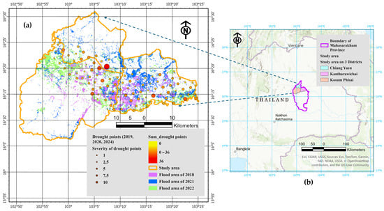
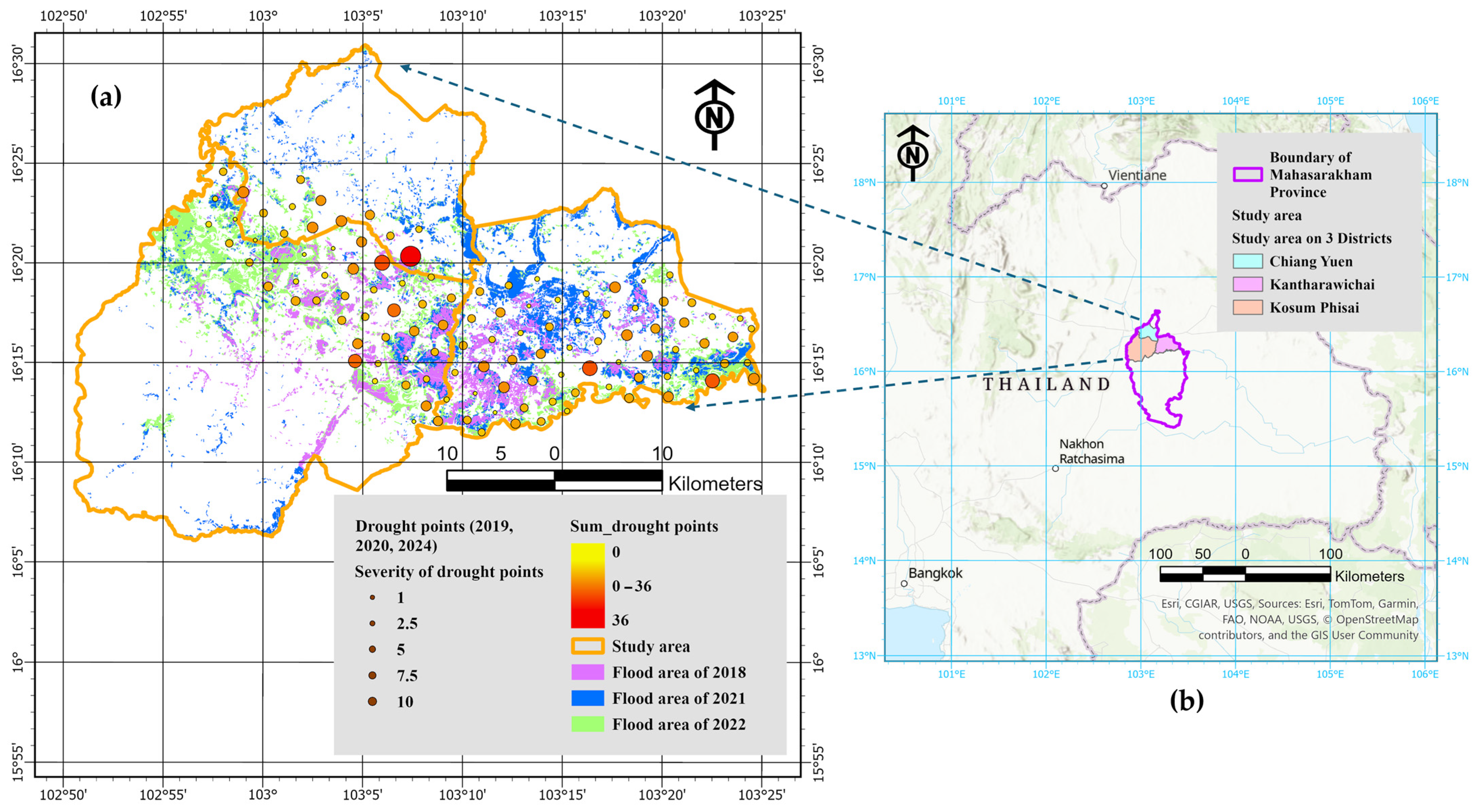
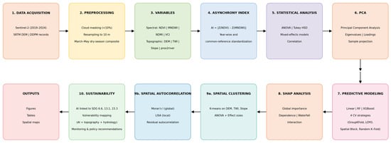
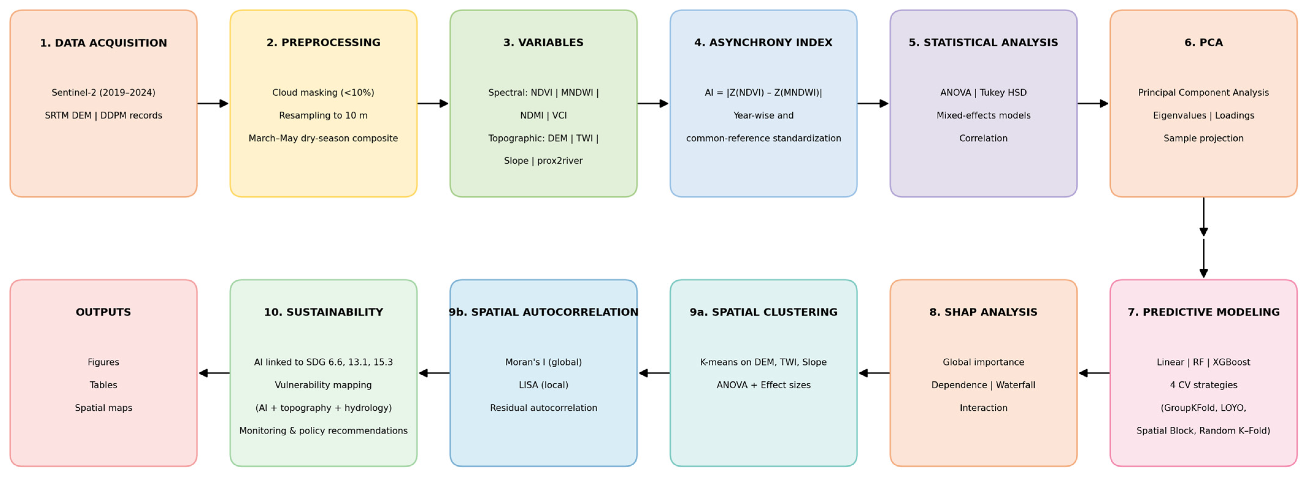
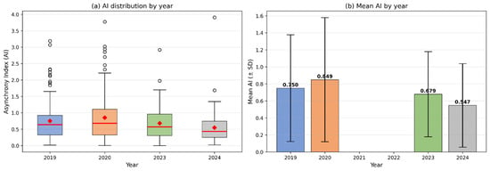
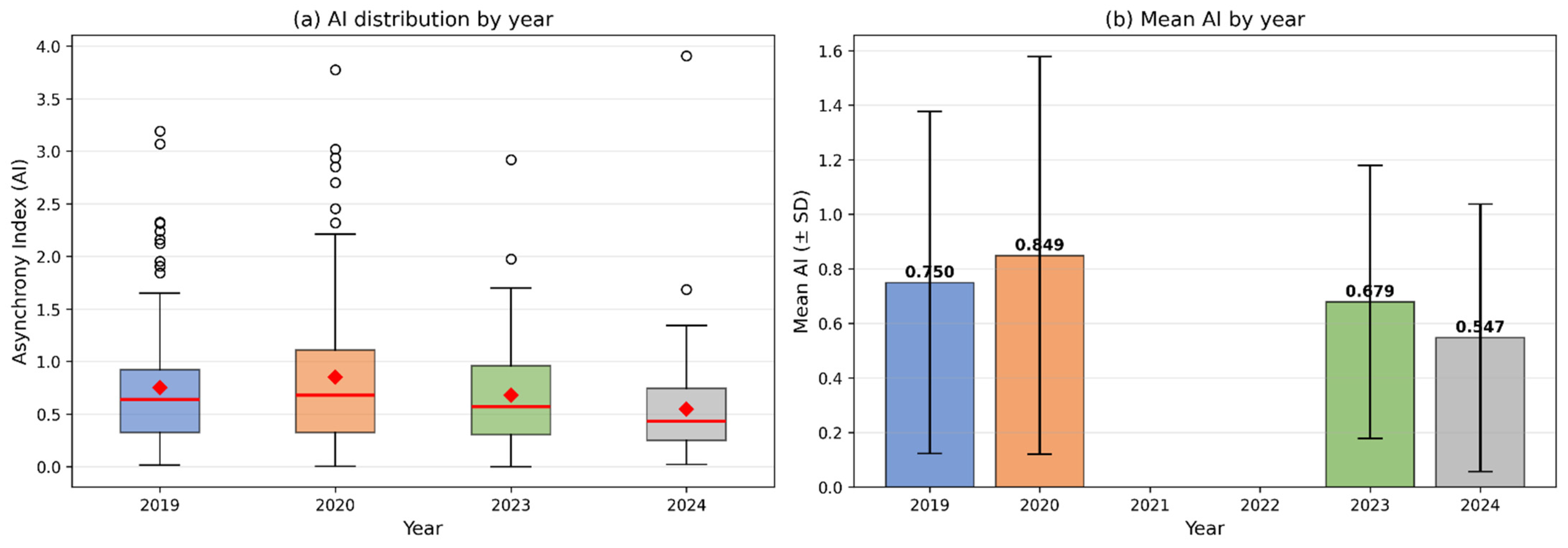
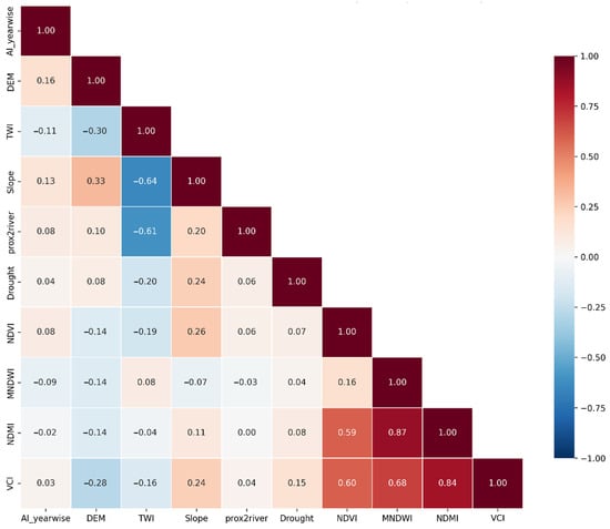
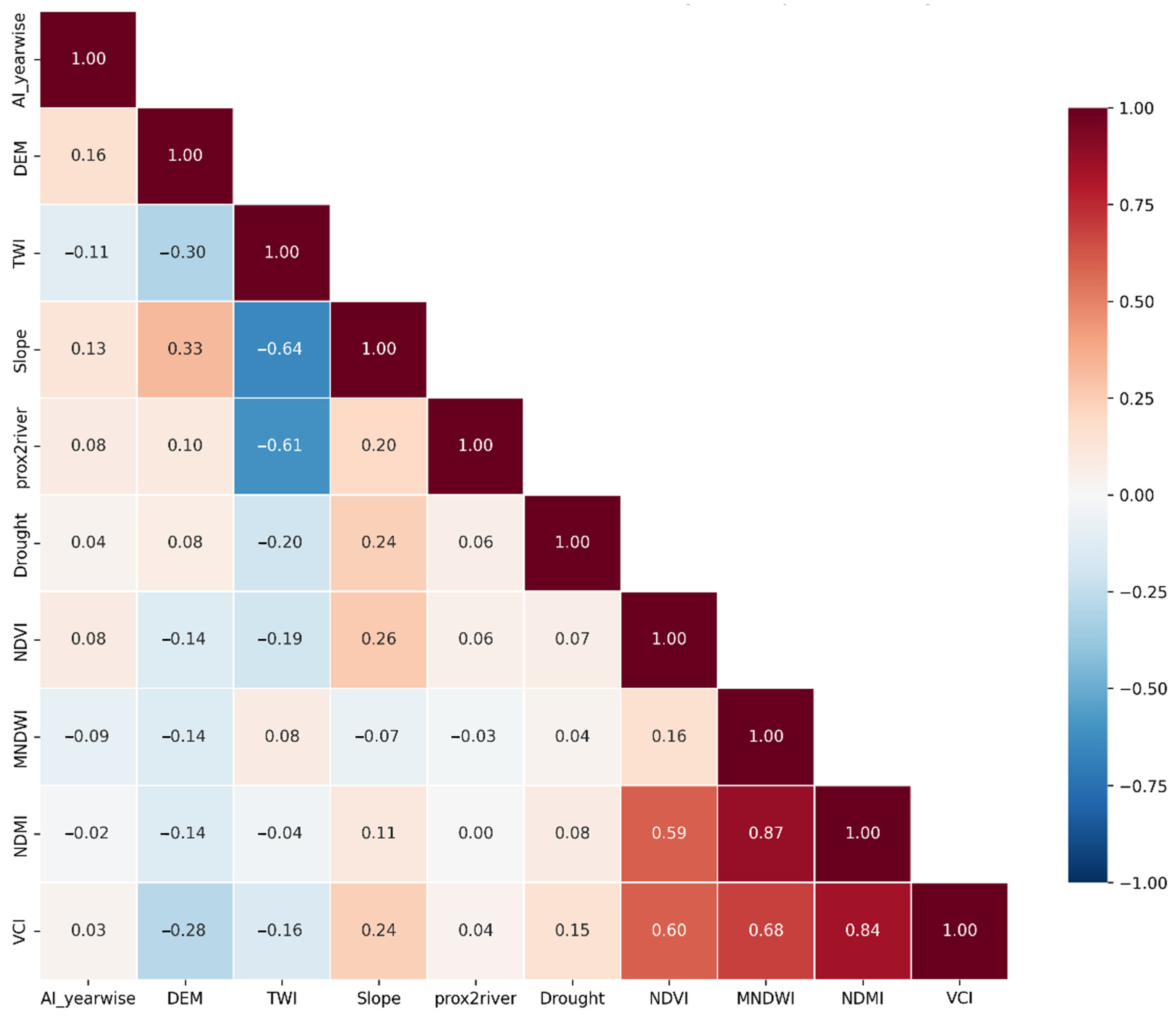
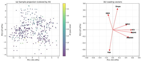
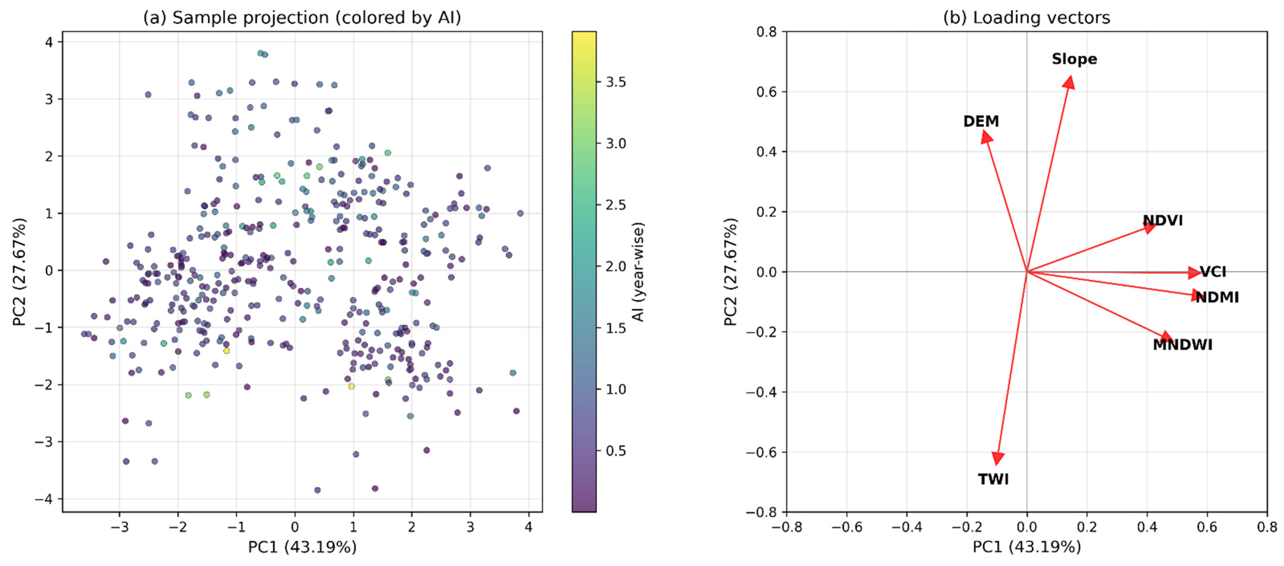
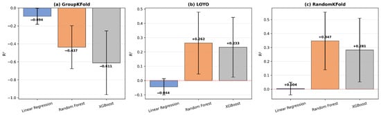
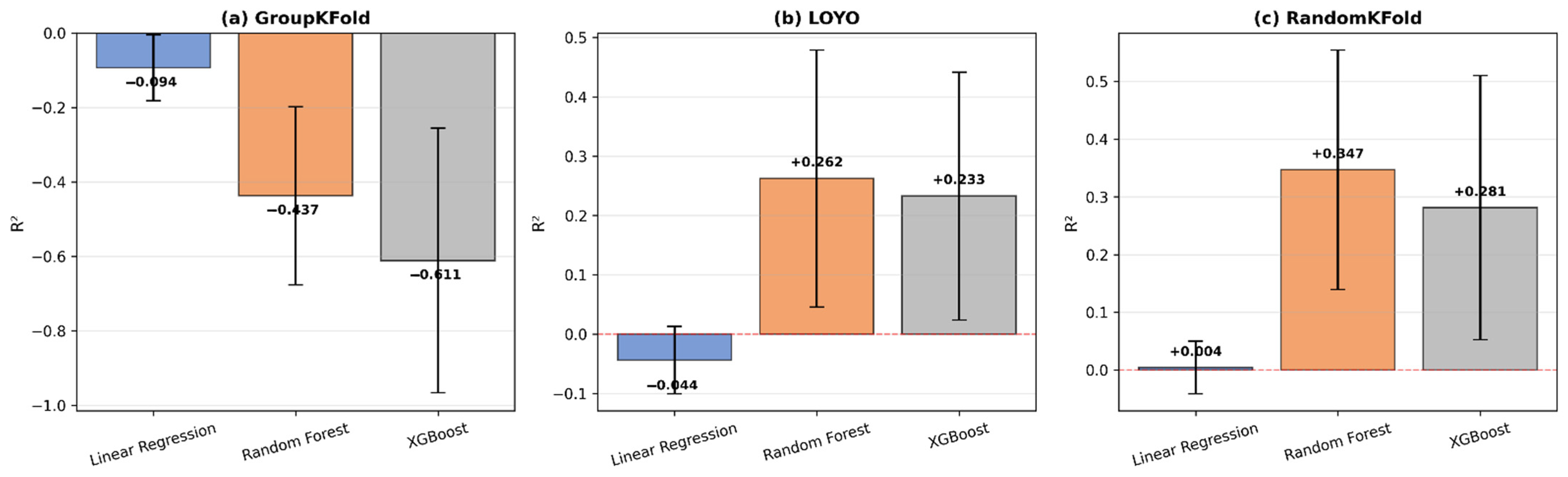
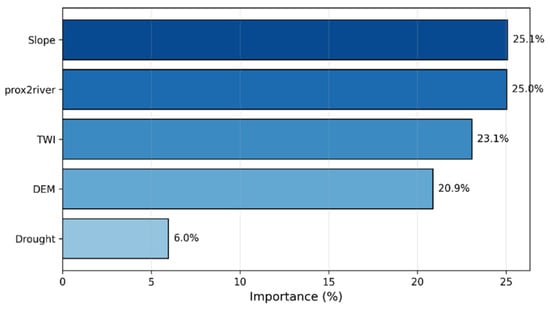
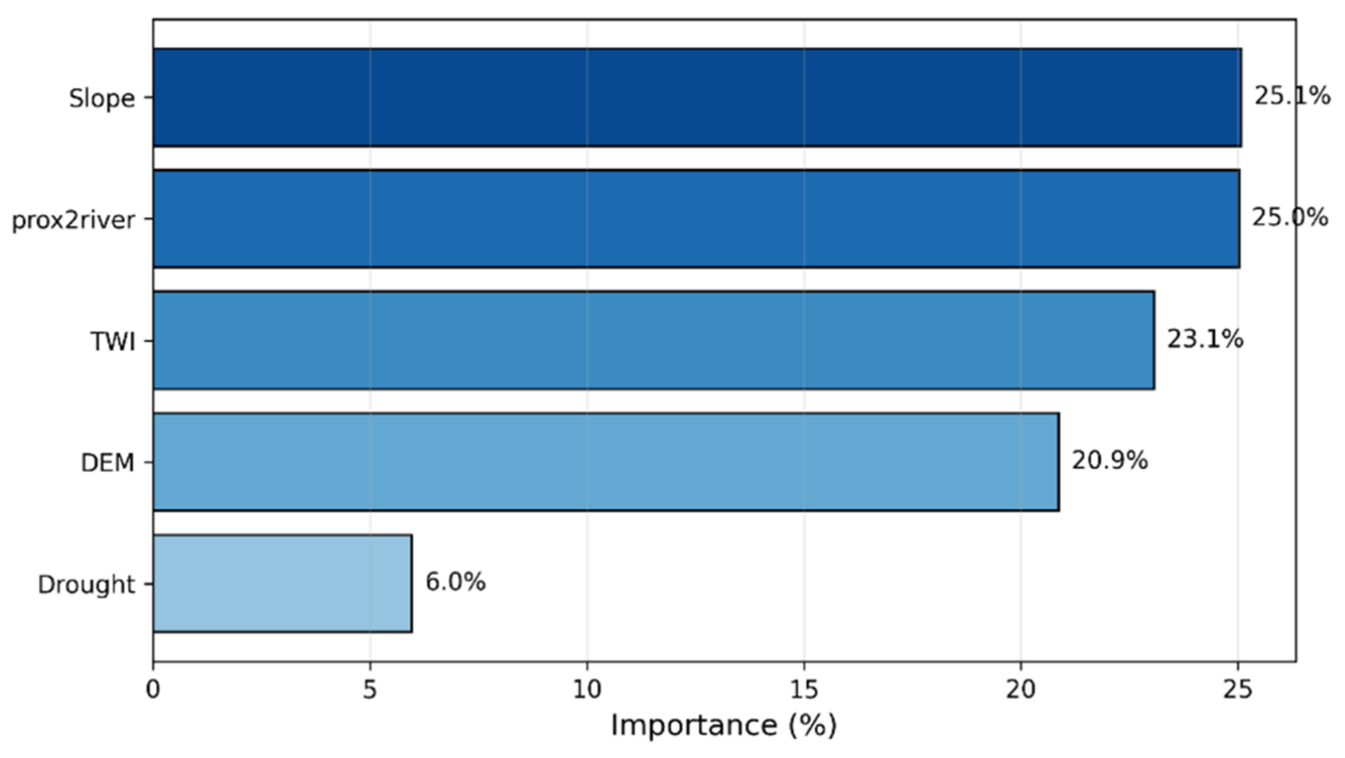
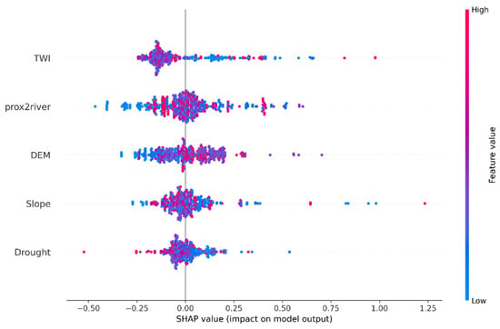
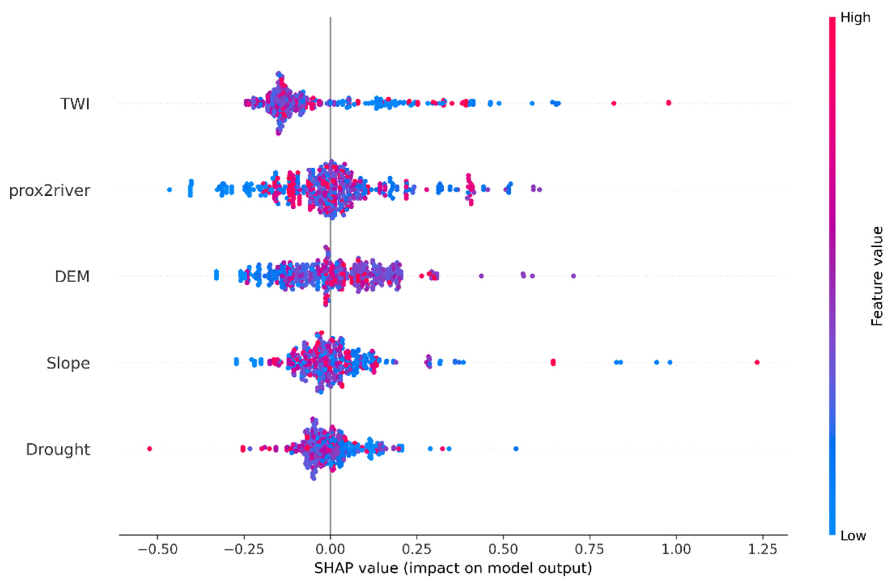
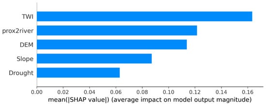
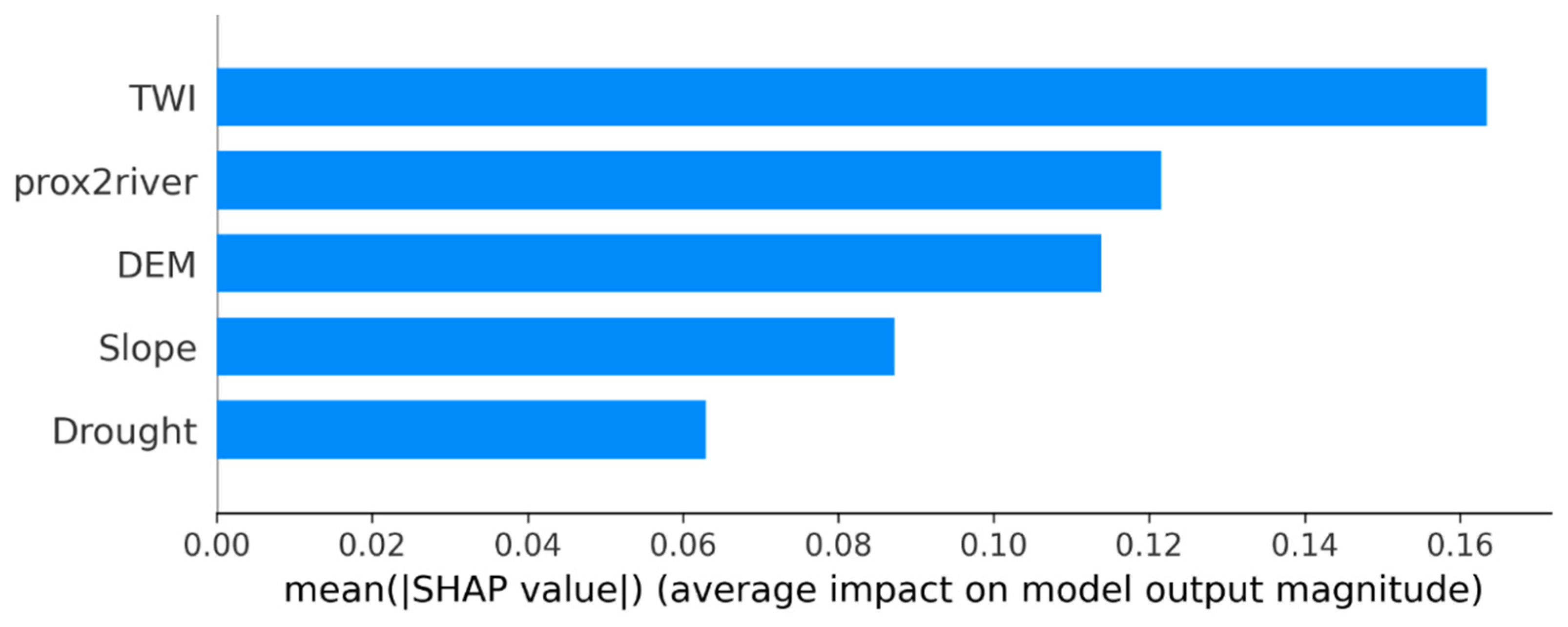
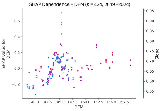
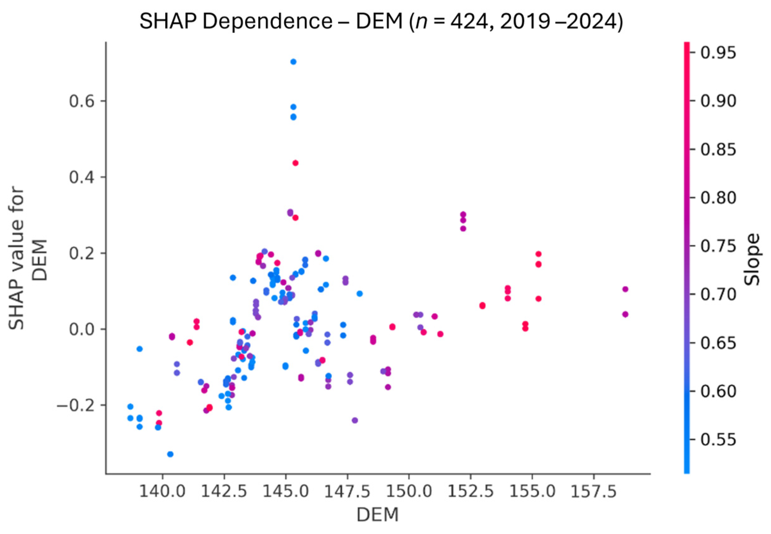
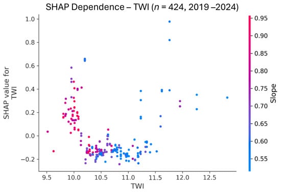
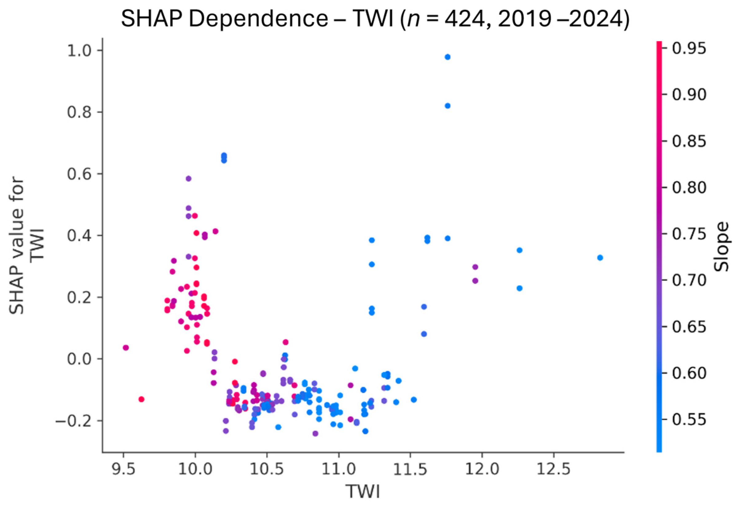
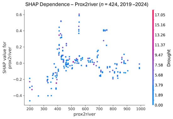
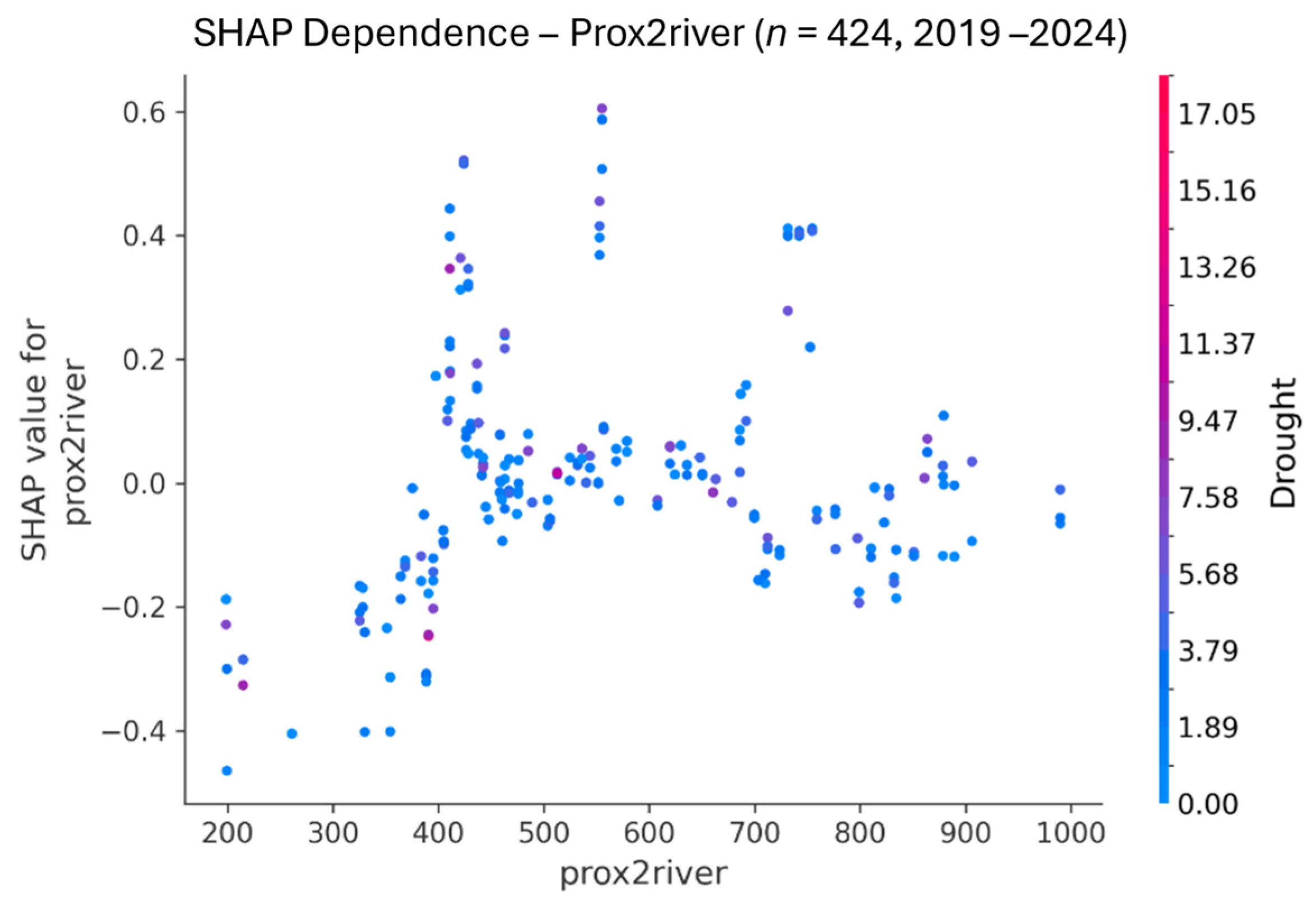
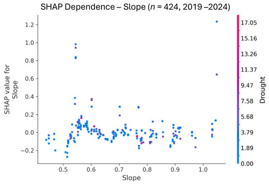
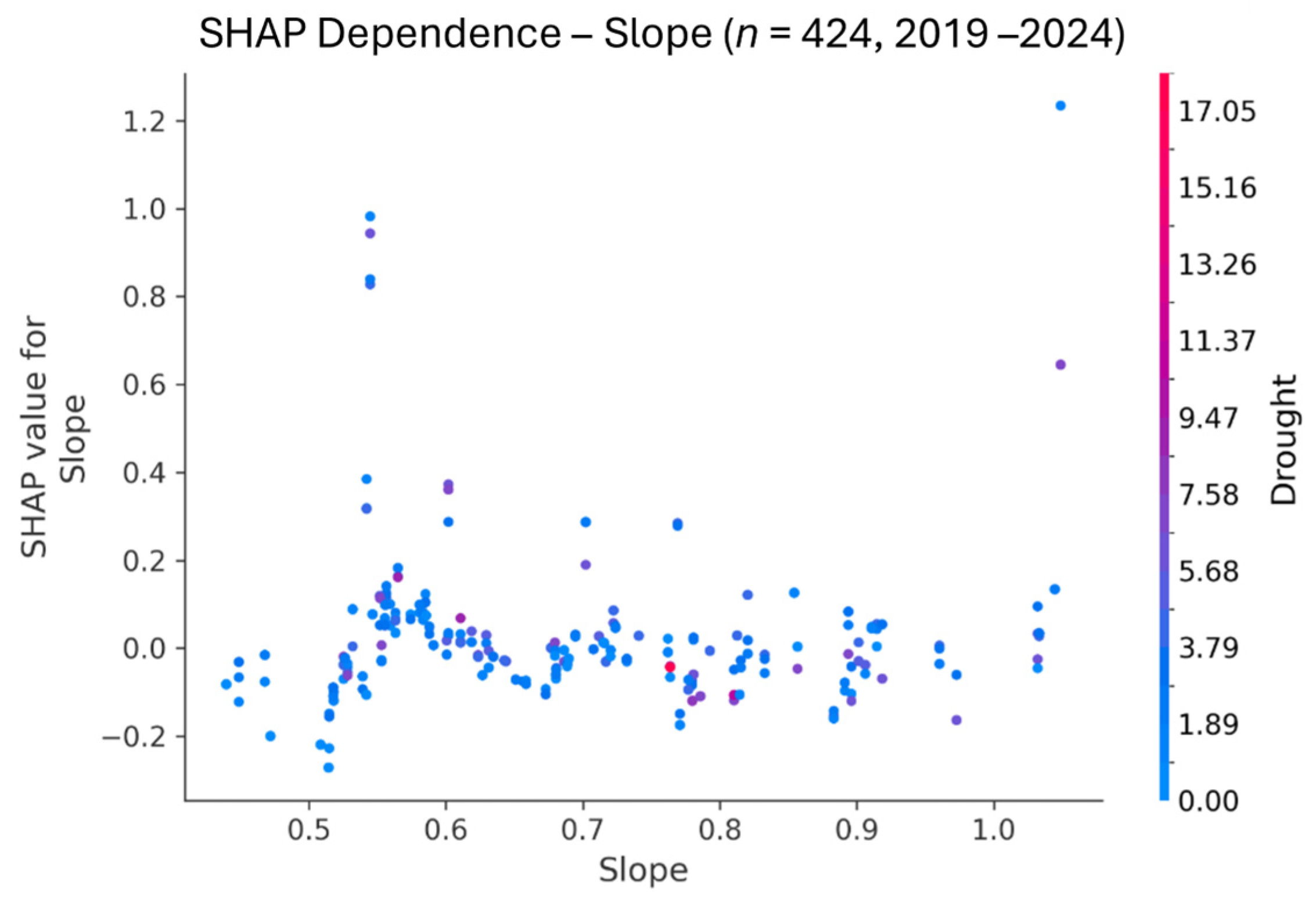
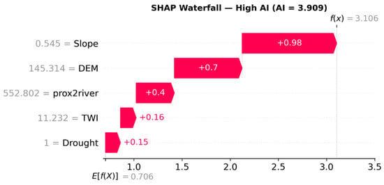
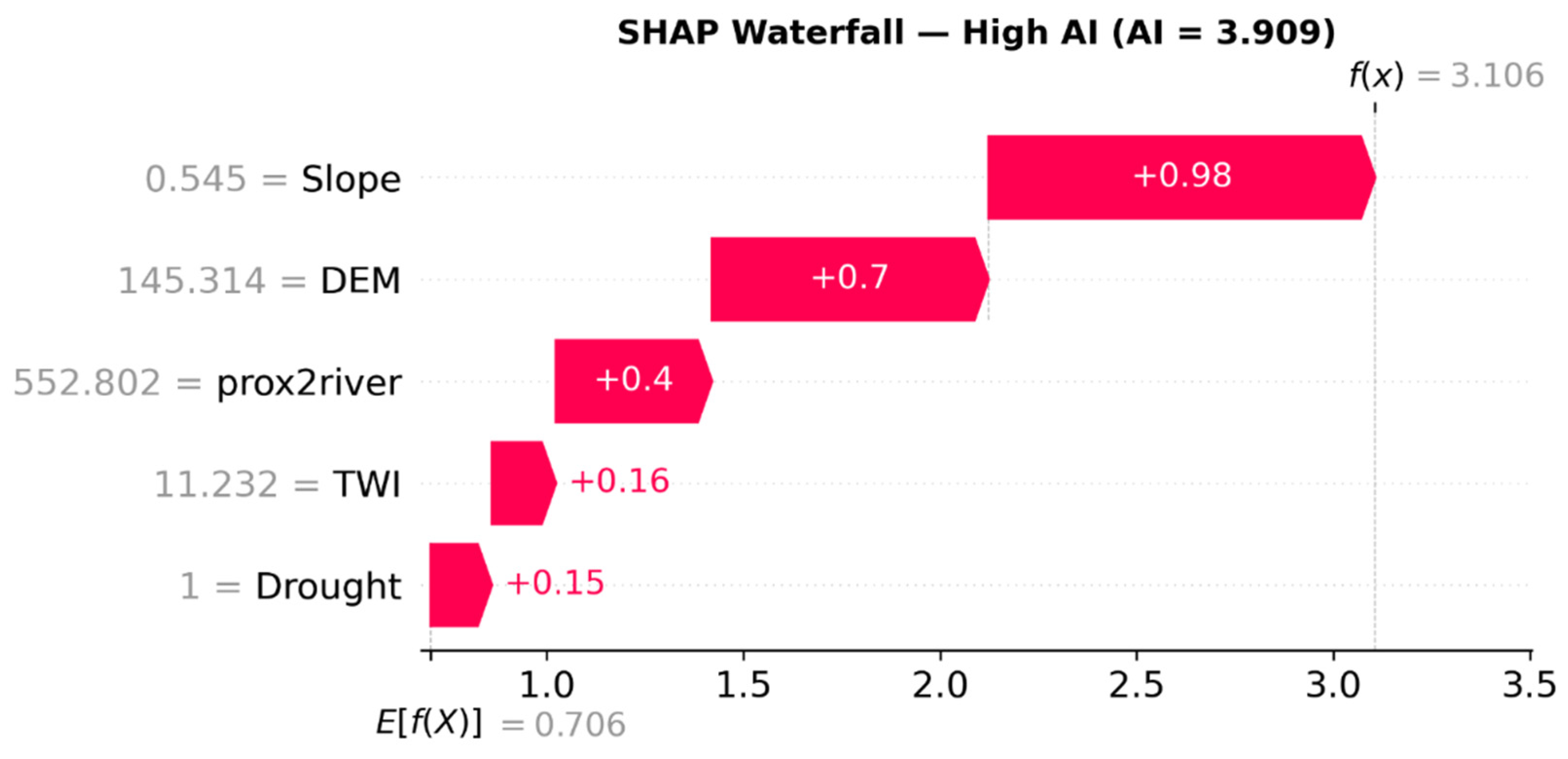
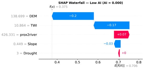
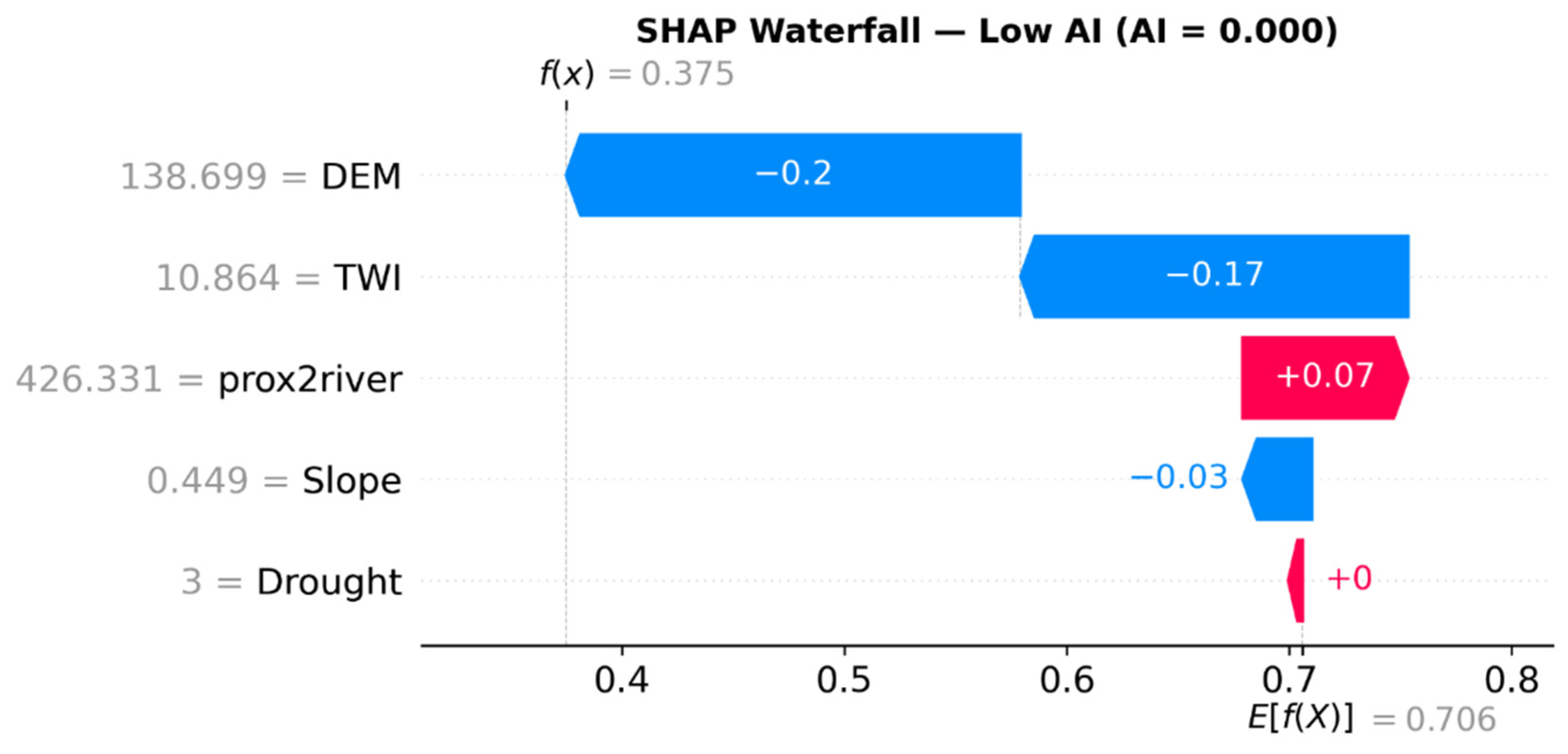
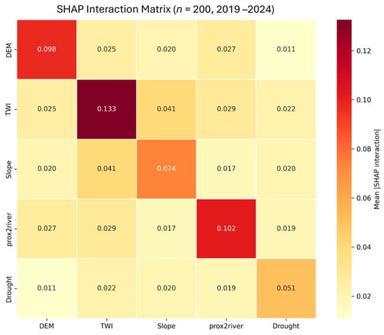
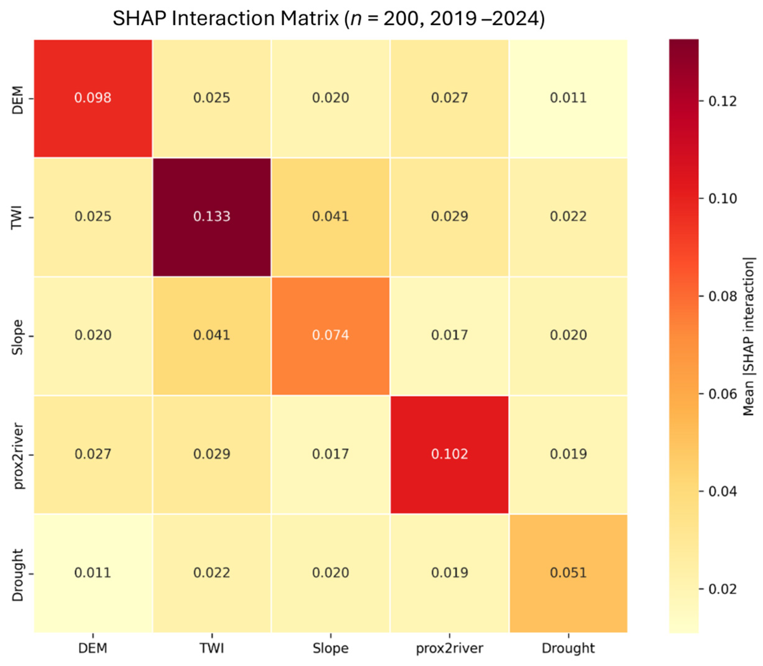
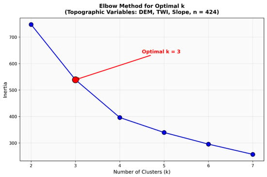
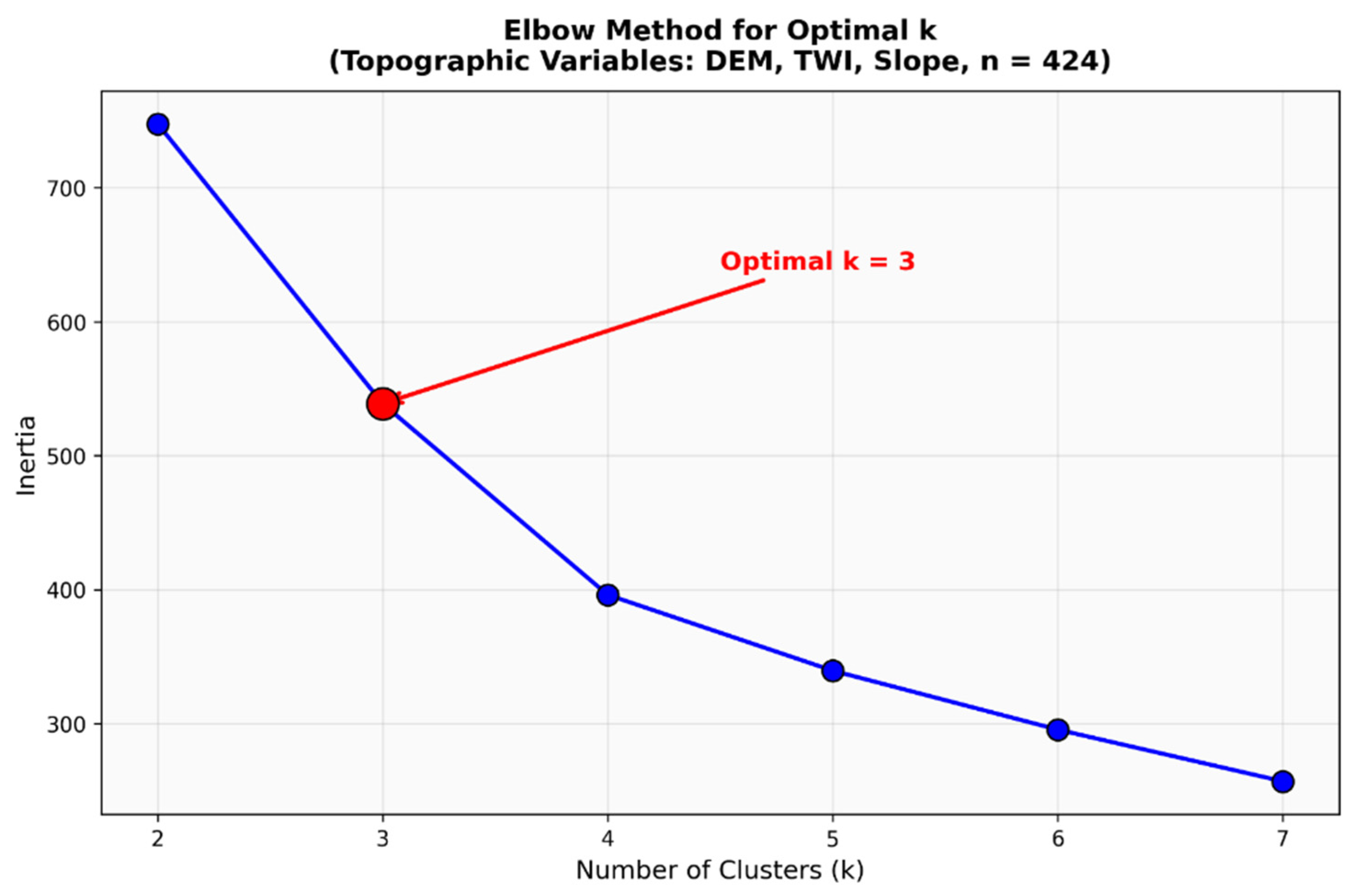
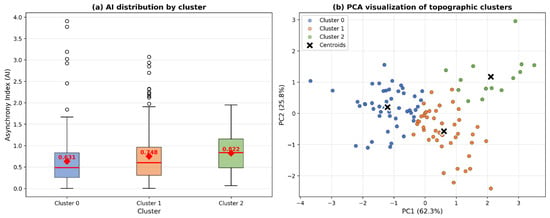
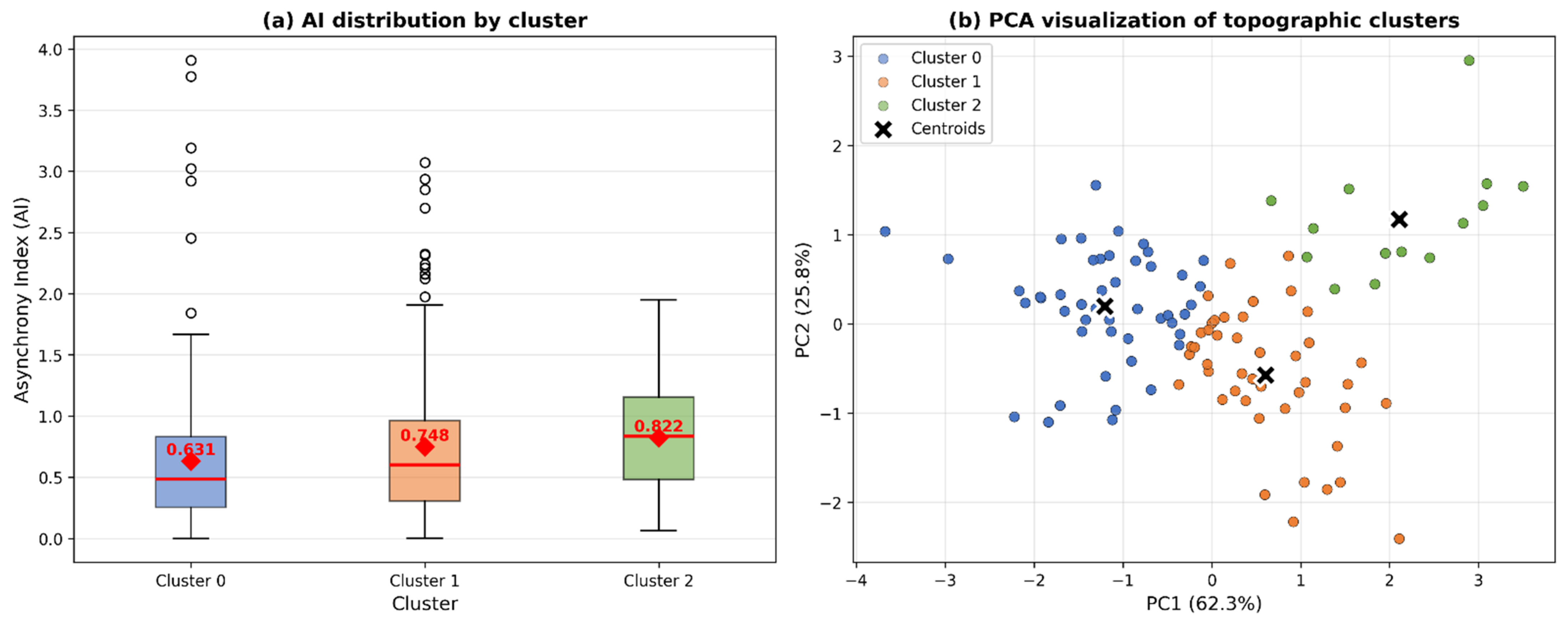
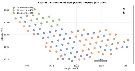
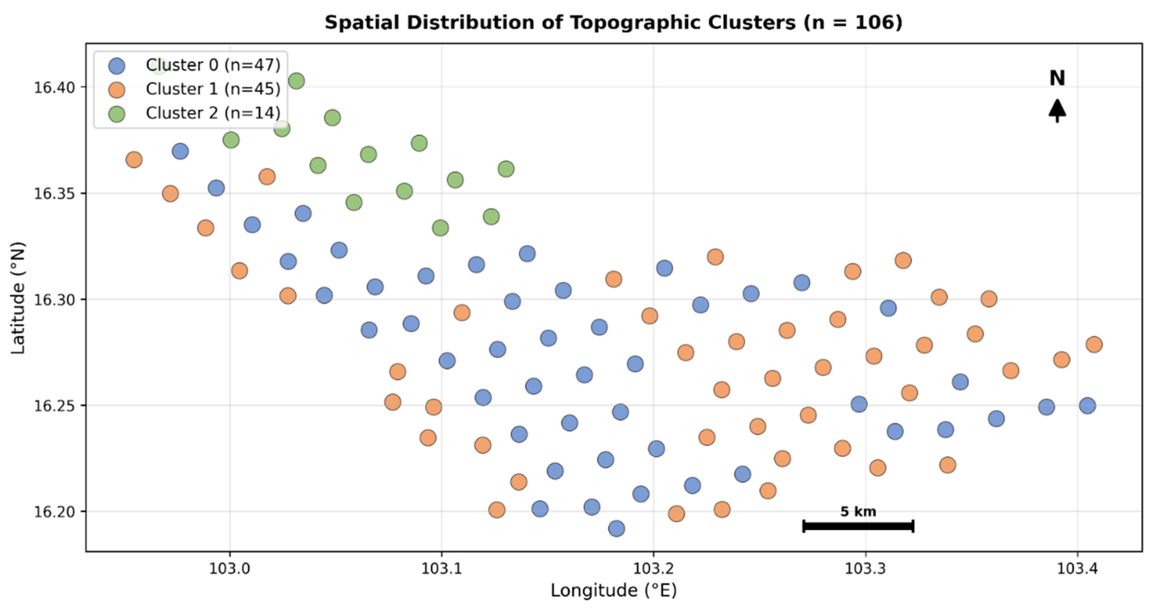
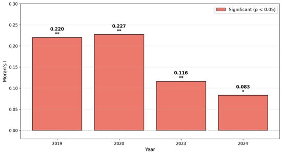
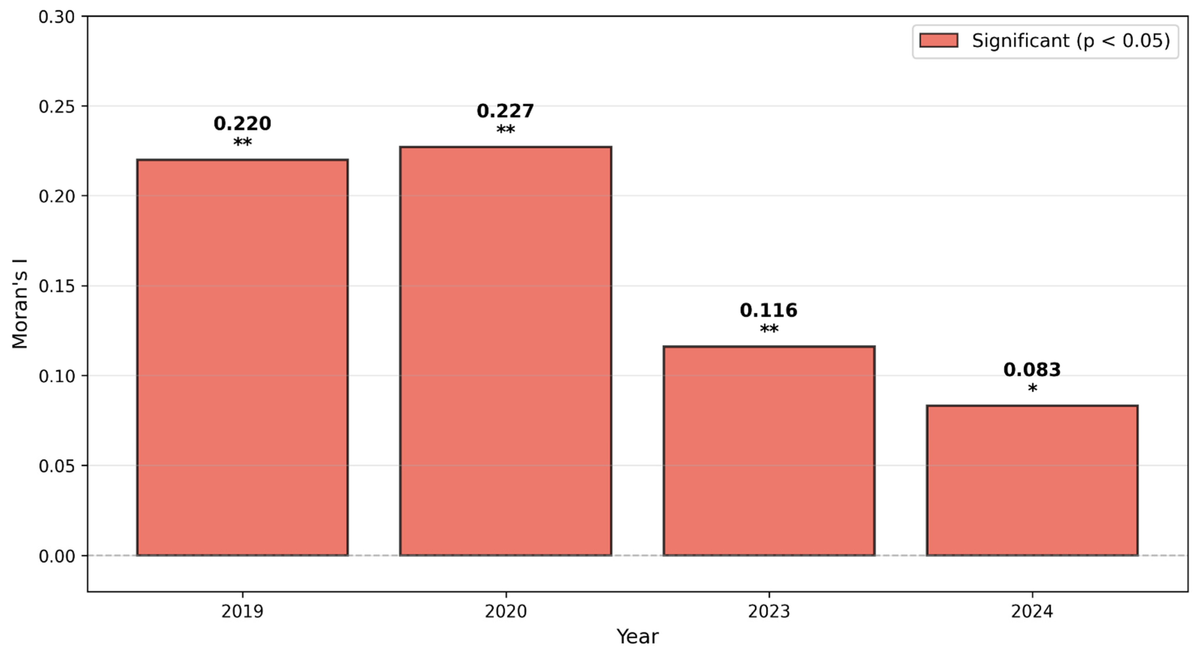
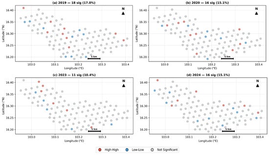
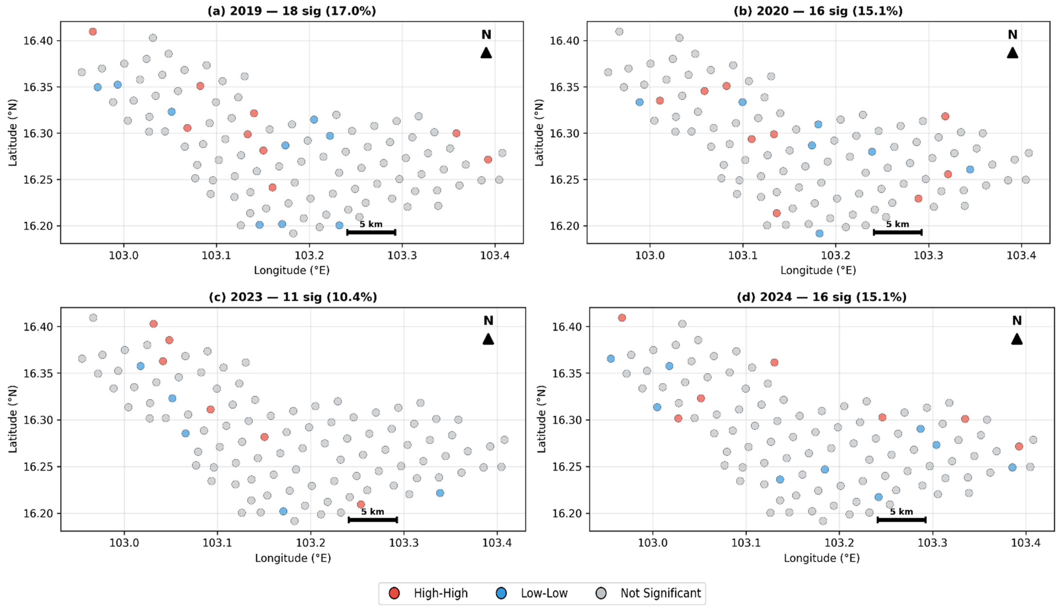
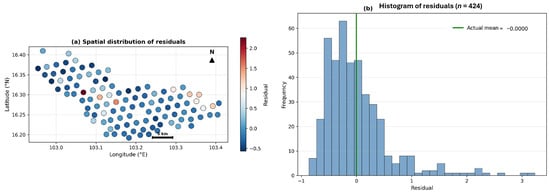
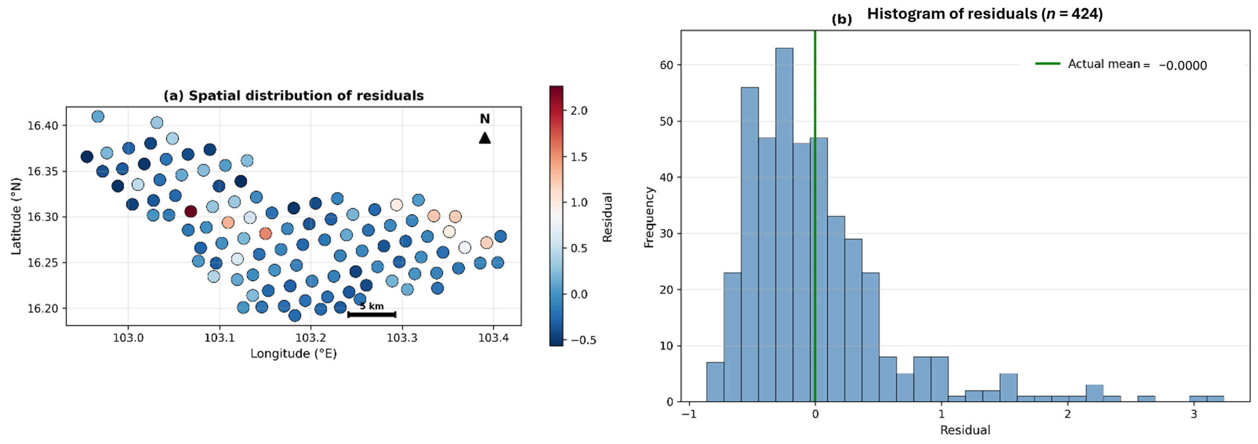
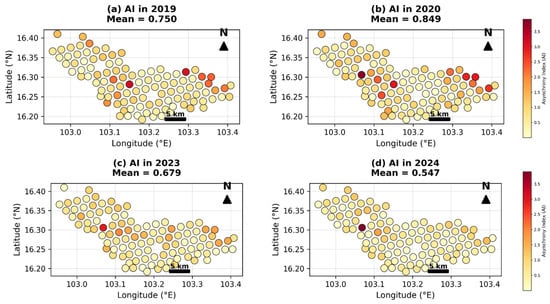
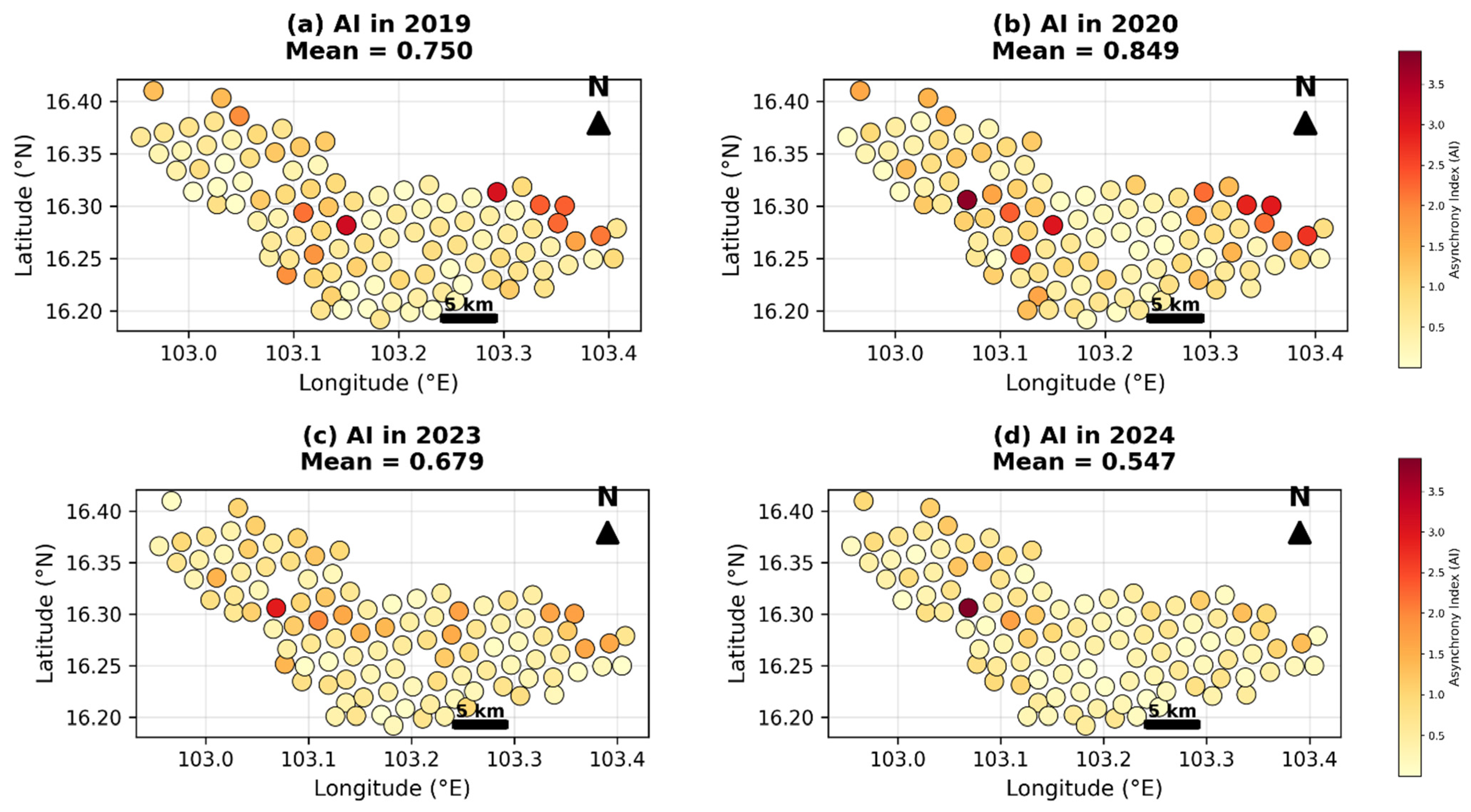
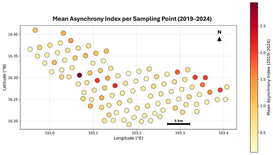
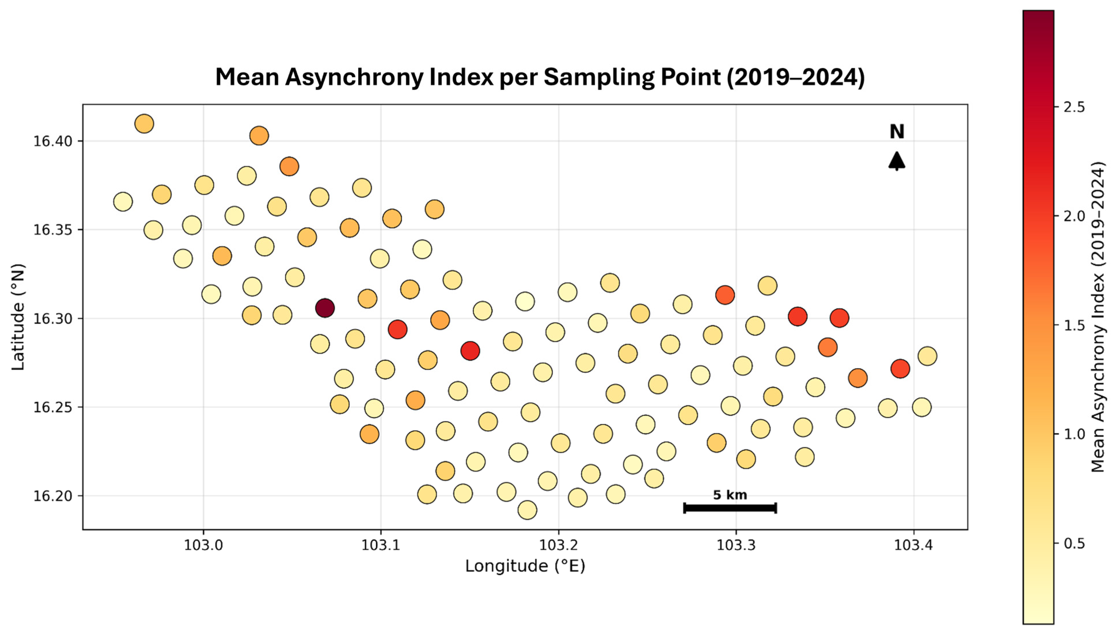

Disclaimer/Publisher’s Note: The statements, opinions and data contained in all publications are solely those of the individual author(s) and contributor(s) and not of MDPI and/or the editor(s). MDPI and/or the editor(s) disclaim responsibility for any injury to people or property resulting from any ideas, methods, instructions or products referred to in the content. |
© 2026 by the authors. Licensee MDPI, Basel, Switzerland. This article is an open access article distributed under the terms and conditions of the Creative Commons Attribution (CC BY) license.