Reliability Estimation for the Inverse Chen Distribution Under Adaptive Progressive Censoring with Binomial Removals: A Framework for Asymmetric Data

Abstract

Traditional reliability methods using fixed removal plans often overlook withdrawal randomness, leading to biased estimates for asymmetric data. This study advances classical and Bayesian frameworks for the inverse Chen distribution, which is suited for modeling asymmetric data under adaptive progressively Type-II censoring with binomial removals. Here, removals post-failure follow a dynamic binomial process, enhancing a more realistic approach for reliability studies. Maximum likelihood estimates are computed numerically, with confidence intervals derived asymptotically. Bayesian approaches employ gamma priors, symmetric squared error loss, and posterior sampling for estimates and credible intervals. A simulation study validates the methods, while two asymmetric real-world applications demonstrate practicality: (1) analyzing diamond sizes from South-West Africa, capturing skewed geological distributions, and (2) modeling failure times of airborne communication transceivers, vital for aviation safety. The flexibility of the inverse Chen in handling asymmetric data addresses the limitations of symmetric assumptions, offering precise reliability tools for complex scenarios. This integration of adaptive censoring and asymmetric distributions advances reliability analysis, providing robust solutions where traditional approaches falter.

1. Introduction

Modeling real-world data is a critical task in modern research, necessitating the use of appropriate statistical probability distributions that accurately capture the underlying shape of the data. Such distributions enable researchers to estimate key population characteristics and derive essential functions from the sampled data. The shape of the data refers not only to its distribution but also to the behavior of its failure rate or hazard rate function (HRF). In the statistical literature, numerous distributions have been developed, each with unique properties and applications. Among these, the Chen distribution, introduced by Chen [1], stands out as a versatile model. It is particularly useful for modeling data with a bathtub-shaped or increasing HRF, making it a valuable tool for reliability analysis and survival studies. For more details on extensions of the Chen distribution, readers are referred to the works of Zamani et al. [2,3] and Tarvirdizade and Ahmadpour [4]. Recently, Srivastava and Srivastava [5] proposed the inverse Chen (IC) distribution, an inverted variant of the Chen distribution. This new distribution extends the applicability of the Chen model to diverse data patterns. Following its introduction, Agiwal [6] conducted a comprehensive investigation to explore and analyze the properties of the IC distribution, offering some of its theoretical foundations and practical utility. Many real-world reliability data sets demonstrate asymmetric behavior, which traditional symmetric models cannot accurately capture. The inverse Chen distribution offers a flexible framework for modeling skewed lifetime data, making it suitable for such situations.

Suppose the random variable X follows the Chen distribution. Then, the random variable $Y=X^{-1}$ follows the IC distribution. The probability density function (PDF) and cumulative distribution function (CDF) can be expressed, respectively, as

$$f(y;\alpha ,\beta )=\alpha \beta y^{-(1+\beta )}exp\left[y^{-\beta }+\alpha \omega (y;\beta )\right],y>0$$

(1)

and

$$F(y;\alpha ,\beta )=exp\left[\alpha \omega (y;\beta )\right],$$

(2)

where $\omega (y;\beta )=1-e^{y^{-\beta }}$ and $\alpha >$ and $\beta >0$ are the model parameters. Two other essential functions associated with the random variable Y are the reliability function (RF) and the HRF. These functions can be expressed, respectively, at a specific time $y_0$ as

$$R(y_0;\alpha ,\beta )=1-exp\left[\alpha \omega (y_0;\beta )\right]$$

(3)

and

$$h(y_0;\alpha ,\beta )={\displaystyle \frac{\alpha \beta y_0^{-(1+\beta )}{e}^{y_0^{-\beta }}}{exp\left[-\alpha \omega (y_0;\beta )\right]-1}}.$$

(4)

Agiwal [6] noted that the IC distribution is well suited for modeling data with an upside-down bathtub shape. Additionally, Alotaibi et al. [7] pointed out that the HRF of the IC distribution is highly flexible, capable of accommodating not only an upside-down bathtub shape but also increasing and decreasing patterns. Research on the IC distribution remains relatively limited, with only a few studies investigating its applications and properties. Among these, Kumar et al. [8] explored inferences for two IC populations using joint Type-II censored data. Additionally, Alotaibi et al. [7] investigated the estimation of the stress–strength index under an adaptive progressive Type-II censoring (APTIIC) scheme.

In reliability studies, the presence of censored data is prevalent due to the incomplete information regarding event times for all test units. Censoring serves as a mechanism to effectively manage both time and costs, making it beneficial for the assessment of reliable products as well as contemporary items. A widely employed approach is progressive Type-II censoring (PTIIC), which facilitates the removal of select operational items that can be used for subsequent research endeavors. The PTIIC plan enables researchers to remove live items from the test based on a predefined removal pattern. For further details on this scheme, readers can refer to Balakrishnan et al. [9], Kundu [10], Ng et al. [11], Ghanbari et al. [12], and AL-Zaydi [13]. Ng et al. [14] introduced a more flexible censoring strategy called the APTIIC scheme, with the conventional PTIIC strategy being a special case. This approach ensures the test concludes once the predetermined number of failures is reached, while keeping the total test duration close to a prefixed optimal time, denoted by $\tau$. The APTII scheme can be described as follows: Suppose n identical items are placed on a life test at time zero with progressive censoring plan $\mathbf{S}=(S_1,S_2,\dots ,S_m)$, where m represents the desired number of observed failures. As the experiment progresses, the researcher removes $S_i$ items randomly from the remaining units immediately after recording the i-th failure time, denoted as $Y_{i:m:n}$, for $i=1,\dots ,m$. This plan has two possible ways to conclude the experiment.

• First Scenario: If $Y_{m:m:n}<\tau$, the experiment terminates at $Y_{m:m:n}$, aligning with the conventional PTIIC strategy.
• Second Scenario: If $\tau$ occurs before $Y_{m:m:n}$, the removal pattern is adjusted by setting $S_i=0,i=d+1,\dots ,m-1$ for $i=d+1,\dots ,m-1$, where d is the number of failures observed before the threshold $\tau$. At $Y_{m:m:n}$, all remaining items are removed, i.e., $S^{\ast }=n-m-{\sum }_{i=1}^d{S}_i$.

In recent years, numerous authors have adopted the APTIIC plan to explore various estimation challenges for lifetime distributions, for instance, Panahi and Moradi [15], Kohansal and Shoaee [16], Helu [17], Sharma and Kumar [18], and Kumari et al. [19]. Let $\underline{\mathrm{y}}$ represent an APTIIC sample obtained from the IC population. Thus, the joint likelihood function, ignoring the constant term, can be expressed as

$$L_1\left(\mathit{\phi }\right|\underline{\mathrm{y}})=\prod _{i=1}^{m}f(y_i;\mathit{\phi })\prod _{i=1}^d{[1-F(y_i;\mathit{\phi })]}^{S_i}{[1-F(y_m;\mathit{\phi })]}^{S^{\ast }},$$

(5)

where $y_i$ is the observed realization of $Y_{i:m:n},i=1,\dots ,m$, and $\mathit{\phi }={(\alpha ,\beta )}^{\top }$.

The APTIIC plan operates under the assumption that the removal pattern during the test is predetermined. However, in practical scenarios, the removal pattern may occur randomly. Yuen and Tse [20] highlighted that in some investigations, investigators might find it inappropriate or unsafe to continue examining certain tested units, irrespective of their failure status. In such circumstances, the removal of units after each failure is carried out in a random manner. This approach has attracted considerable attention from researchers, who seek to investigate the influence of random removal on the effectiveness and efficiency of estimation techniques, see, for example, Tse et al. [21], Wu et al. [22], and Elbatal et al. [23]. Under the APTIIC framework, Elshahhat and Nassar [24] suggested the APTIIC with binomial removals (APTIIC-BR) and discussed the estimation concerns associated with the Weibull lifetime model. According to Elshahhat and Nassar [24], the joint probability of $S_i=s_i,i=1,\dots ,d$ can be expressed as follows:

$$L_2\left(\mathbf{S}=\mathbf{s};\theta \right)=C{\theta }^{{\eta }_1}{(1-\theta )}^{{\eta }_2},$$

(6)

where $0<\theta <1$ is the binomial distribution parameter, $C={\prod }_{i=1}^d\left({\displaystyle \genfrac{}{}{0pt}{}{n_i^{\ast }}{s_i}}\right)$, $n_i^{\ast }=n-m-{\sum }_{r=1}^{i-1}{s}_r$, ${\eta }_1={\sum }_{i=1}^d{s}_i$, and ${\eta }_2=d(n-m)-{\sum }_{i=1}^d(d-i+1)s_i$. By integrating the likelihood function in (5) with the joint probability in (6), the full likelihood function for the parameter vector and the complete likelihood function of the model parameter vector $\mathit{\phi }$ and the binomial distribution parameter $\theta$ can be expressed as follows:

$$L(\mathit{\phi },\theta ;\underline{\mathrm{y}},\mathbf{s})=L_1\left(\mathit{\phi }\right|\underline{\mathrm{y}},\mathbf{S}=\mathbf{s})L_2\left(\mathbf{S}=\mathbf{s};\theta \right).$$

(7)

The primary motivation for this work lies in the critical role of the censoring plan in reliability analysis. Although the traditional PTIIC scheme has been widely used, it lacks flexibility because the number of units to be removed is fixed in advance. The APTIIC plan addresses this limitation by allowing removal decisions to be adjusted dynamically based on observed failures, thereby optimizing data collection. An additional advancement involves modeling unit removals using a binomial distribution, which introduces a probabilistic element that better captures real-world variability, unlike the deterministic nature of earlier methods. This combination of adaptability and randomness not only enhances the data collection process but also improves statistical efficiency. The second motivation arises from the importance of selecting an appropriate lifetime distribution in reliability engineering and survival analysis, where accurate modeling of failure mechanisms is essential. While traditional distributions such as the Weibull, exponential, and gamma have been widely used, their monotonic hazard rate structures often limit their effectiveness in capturing real-world failure behaviors, which frequently exhibit non-monotonic patterns. The IC distribution, known for its upside-down bathtub-shaped hazard function, addresses this limitation by providing a better fit for lifetime data with unimodal hazard rates. This motivates the investigation of the IC distribution as a promising addition to the suite of models available for analyzing data with unimodal failure patterns. Despite its potential, estimating the reliability metrics of the IC distribution has received limited attention, particularly in the context of modern censoring schemes, warranting further exploration.

As a result, this study aims to investigate the estimation of the IC distribution’s model parameters, the binomial distribution parameter, and two key reliability measures using data generated under the APTIIC-BR scheme. The main contributions of this study can be summarized as follows: (1) Investigating the parameter estimation and reliability metrics of the IC distribution within the APTIIC-BR framework, which is particularly well suited for resource-constrained environments. (2) Providing practical guidance for researchers and practitioners by comparing classical and Bayesian estimation methods, helping to identify the most appropriate approach for analyzing data with the IC distribution. (3) Demonstrating the real-world applicability of the proposed model, censoring scheme, and estimation techniques through the analysis of real data sets. To carry out this study, we employ the maximum likelihood method to derive point estimates and construct approximate confidence intervals (ACIs). In parallel, Bayesian estimates are obtained using the squared error (SE) loss function and Markov Chain Monte Carlo (MCMC) techniques, accompanied by symmetric Bayesian credible intervals (BCIs). The effectiveness of these estimation approaches is assessed through an extensive simulation study and the analysis of two real-world data sets. This analysis underscores the utility of the proposed approaches in addressing reliability estimation challenges.

The remainder of this study is structured as follows: Section 2 focuses on the classical estimation method, providing detailed discussions on point and interval estimations for the model parameters, the binomial distribution parameter, and the two reliability measures. Section 3 considers the Bayesian framework, presenting the derivation of Bayes point estimates and the construction of the BCIs. Section 4 outlines the simulation study, including the design of the simulation experiments and a comprehensive analysis of the numerical results to evaluate the performance of the proposed estimation methods. Section 5 applies the proposed methods to two real-world data sets, demonstrating their practical utility and effectiveness in real-life scenarios. Finally, Section 6 concludes this paper by summarizing the key findings.

2. Classical Estimation

In this section, we focus on the maximum likelihood estimation approach, a key classical method, to estimate the parameters $\alpha ,\beta$, the binomial parameter $\theta$, the RF, and the HRF of the IC distribution based on the APTIIC-BR data.

2.1. Point Estimation

Let $\underline{\mathrm{y}}$ be an APTIIC-BR sample characterized by the removal pattern $\mathbf{S}=(S_1,\dots ,S_d$$,0,\dots ,0,S^{\ast })$, drawn from the IC population with the PDF and CDF, as given by (1) and (2), respectively. Since the the joint likelihood function of the model parameters is independent of the binomial parameter $\theta$, we can write the likelihood function of the unknown parameter vector $\mathit{\phi }$ using (5) as follows:

$$\begin{array}{ccc}\hfill L_1\left(\mathit{\phi }\right|\underline{\mathrm{y}},\mathbf{S}=\mathbf{s})& =& {\alpha }^m{\beta }^{m}exp\left\{(\beta +1)\sum _{i=1}^{m}log\left(y_i\right)+\sum _{i=1}^m{y}_i^{\beta }+\alpha \sum _{i=1}^m\omega (y_i;\beta )\right\}\hfill \\ & \times & exp\left\{\sum _{i=1}^d{s}_{i}log\left[\varpi (y_i;\mathit{\phi })\right]+s^{\ast }log\left[\varpi (y_m;\mathit{\phi })\right]\right\},\hfill \end{array}$$

(8)

where $y_i=y_i^{-1}$ for simplicity, $\omega (y_i;\beta )=1-e^{y_i^{\beta }}$, and $\varpi (y_i;\mathit{\phi })=1-e^{\alpha \omega (y_i;\beta )}$. The objective function to be maximized is derived by taking the natural logarithm of (8), which is expressed as

$$\begin{array}{ccc}\hfill l_1\left(\mathit{\phi }\right|\underline{\mathrm{y}},\mathbf{S}=\mathbf{s})& =& mlog\left(\alpha \right)+mlog\left(\beta \right)+(\beta +1)\sum _{i=1}^{m}log\left(y_i\right)+\sum _{i=1}^m{y}_i^{\beta }+\alpha \sum _{i=1}^m\omega (y_i;\beta )\hfill \\ & +& \sum _{i=1}^d{s}_{i}log\left[\varpi (y_i;\mathit{\phi })\right]+s^{\ast }log\left[\varpi (y_m;\mathit{\phi })\right].\hfill \end{array}$$

(9)

By setting the first-order partial derivatives of (9) with respect to $\alpha$ and $\beta$ to zero, the two normal equations that must be solved simultaneously to obtain the classical estimators are

$$\begin{array}{ccc}\hfill {\displaystyle \frac{\partial l_1\left(\mathit{\phi }\right|\underline{\mathrm{y}},\mathbf{S}=\mathbf{s})}{\partial \alpha }}& =& {\displaystyle \frac{m}{\alpha }}+\sum _{i=1}^m\omega (y_i;\beta )+\sum _{i=1}^d{s}_i{\varpi }_1(y_i;\mathit{\phi })+s^{\ast }{\varpi }_1(y_m;\mathit{\phi })=0\hfill \end{array}$$

(10)

and

$$\begin{array}{ccc}\hfill {\displaystyle \frac{\partial l_1\left(\mathit{\phi }\right|\underline{\mathrm{y}},\mathbf{S}=\mathbf{s})}{\partial \beta }}& =& {\displaystyle \frac{m}{\beta }}+\sum _{i=1}^{m}log\left(y_i\right)(1+y_i^{\beta })-\alpha \sum _{i=1}^m{\omega }_1(y_i;\beta )-\sum _{i=1}^d{s}_i{\varpi }_2(y_i;\mathit{\phi })-s^{\ast }{\varpi }_2(y_m;\mathit{\phi })=0,\hfill \end{array}$$

(11)

where ${\varpi }_1(y_i;\mathit{\phi })={\displaystyle \frac{\omega (y_i;\beta )}{1-e^{-\alpha \omega (y_i;\beta )}}}$, ${\omega }_1(y_i;\beta )=y_i^{\beta }log\left(y_i\right)e^{y_i^{\beta }}$, and ${\varpi }_2(y_i;\mathit{\phi })={\displaystyle \frac{\alpha y_i^{\beta }log\left(y_i\right)e^{y_i^{\beta }}}{1-e^{-\alpha \omega (y_i;\beta )}}}$.

To derive the maximum likelihood estimates (MLEs) of the parameters $\alpha$ and $\beta$, denoted as $\widehat{\alpha }$ and $\widehat{\beta }$, the system of equations specified in (10) and (11) must be solved. However, due to the complexity of these equations, a closed-form analytical solution is not feasible. Consequently, a computational approach is necessary to numerically approximate the solutions. Among the available numerical methods, we recommend using the Newton–Raphson iterative technique to acquire the required estimates.

Using the invariance principle of the maximum likelihood estimation method, we can derive the MLEs of the RF and the HRF by replacing the true parameters $\alpha$ and $\beta$ with their MLEs $\widehat{\alpha }$ and $\widehat{\beta }$, respectively. At a distinct time $y_0$, the MLEs of the RF $R\left(y_0\right)=R(y_0;\alpha ,\beta )$ and the HRF $h\left(y_0\right)=h(y_0;\alpha ,\beta )$ are given, respectively, by

$$\widehat{R}\left(y_0\right)=1-exp\left[\widehat{\alpha }\omega (y_0;\widehat{\beta })\right]$$

and

$$\widehat{h}\left(y_0\right)={\displaystyle \frac{\widehat{\alpha }\widehat{\beta }{y}_0^{1+\widehat{\beta }}{e}^{y_0^{\widehat{\beta }}}}{exp\left[-\widehat{\alpha }\omega (y_0;\widehat{\beta })\right]-1}},y_0=y_0^{-1}.$$

Regarding the binomial distribution parameter $\theta$, one can simply write the natural logarithm of (6), ignoring the constant term, as given below:

$$l_2\left(\theta \right)={\eta }_{1}log\left(\theta \right)+{\eta }_{2}log(1-\theta ),$$

(12)

By setting ${\displaystyle \frac{d{l}_2\left(\theta \right)}{d\theta }}=0$, we can express the MLE of the parameter $\theta$ as

$$\widehat{\theta }={\displaystyle \frac{{\eta }_1}{{\eta }_1+{\eta }_2}}.$$

2.2. Interval Estimation

Determining the interval ranges for unknown parameters, particularly for reliability measures, is a critical aspect of statistical analysis. In this section, we utilize the asymptotic properties of the MLEs to construct ACIs for the model parameters, the binomial parameter, and the two reliability measures. A significant challenge in constructing the interval ranges lies in deriving the exact expressions for the Fisher information matrix, which is essential for computing the variance–covariance matrix. These expressions involve calculating the expectation of the second-order derivatives of the log-likelihood function (9). To address this, we employ the observed Fisher information matrix, evaluated at the MLEs $\widehat{\alpha }$, $\widehat{\beta }$, and $\widehat{\theta }$, to estimate the variance–covariance matrix. This approach provides a practical way to approximate the required intervals without relying on exact analytical derivations. Let $\mathit{I}(\widehat{\mathit{\phi }},\widehat{\theta })$ refer to the observed Fisher information matrix, where $\widehat{\mathit{\phi }}={(\widehat{\alpha },\widehat{\beta })}^{\top }$. Then, the estimated variance–covariance matrix can be obtained as follows:

$$\begin{array}{ccc}\hfill {\mathit{I}}^{-1}(\widehat{\mathit{\phi }},\widehat{\theta })& =& {\left[\begin{array}{ccc}-{\displaystyle \frac{\partial l_1^2\left(\mathit{\phi }\right|\underline{\mathrm{y}},\mathbf{S}=\mathbf{s})}{\partial {\alpha }^2}}& -{\displaystyle \frac{\partial l_1^2\left(\mathit{\phi }\right|\underline{\mathrm{y}},\mathbf{S}=\mathbf{s})}{\partial \alpha \partial \beta }}& 0\\ & -{\displaystyle \frac{\partial l_1^2\left(\mathit{\phi }\right|\underline{\mathrm{y}},\mathbf{S}=\mathbf{s})}{\partial {\beta }^2}}& 0\\ & & -{\displaystyle \frac{\partial l_2^2\left(\theta \right)}{\partial {\theta }^2}}\end{array}\right]}_{(\mathit{\phi },\theta )=(\widehat{\mathit{\phi }},\widehat{\theta })}^{-1},\hfill \end{array}$$

(13)

where the second derivatives of the log-likelihood functions are given in Appendix A.

Let $\widehat{var}\left(\widehat{\alpha }\right)$, $\widehat{var}\left(\widehat{\beta }\right)$, and $\widehat{var}\left(\widehat{\theta }\right)$ represent the estimated variances corresponding to the MLEs of $\alpha ,\beta$, and $\theta$, respectively. These variances are obtained as the main diagonal elements of the variance–covariance matrix (13). Using the asymptotic normality of the MLEs, i.e., $(\widehat{\mathit{\phi }},\widehat{\theta })\sim N((\mathit{\phi },\theta ),{\mathit{I}}^{-1}(\mathit{\phi },\theta ))$, where ${\mathit{I}}^{-1}(\mathit{\phi },\theta )$ is estimated using (13), the $100\%(1-\epsilon )$ ACIs for the model parameters $\alpha$ and $\beta$ and the binomial distribution parameter $\theta$ can be constructed as

$$\left[\widehat{\alpha }-z_{\epsilon /2}\sqrt{\widehat{var}\left(\widehat{\alpha }\right)},\widehat{\alpha }+z_{\epsilon /2}\sqrt{\widehat{var}\left(\widehat{\alpha }\right)}\right],\left[\widehat{\beta }-z_{\epsilon /2}\sqrt{\widehat{var}\left(\widehat{\beta }\right)},\widehat{\beta }+z_{\epsilon /2}\sqrt{\widehat{var}\left(\widehat{\beta }\right)}\right]$$

and

$$\left[\widehat{\theta }-z_{\epsilon /2}\sqrt{\widehat{var}\left(\widehat{\theta }\right)},\widehat{\theta }+z_{\epsilon /2}\sqrt{\widehat{var}\left(\widehat{\theta }\right)}\right],$$

where $z_{\epsilon /2}$ is the upper $\epsilon /2$ percentile of the standard normal distribution.

In order to construct the ACIs for the RF and the HRF, it is essential to estimate the variances of their MLEs. The delta method, a commonly employed technique for approximating the variance of functions of random variables, can be utilized for this purpose, see Green [25] for more details. Prior to applying the delta method, it is necessary to compute the first-order partial derivatives of the RF and HRF with respect to the model parameters $\alpha$ and $\beta$. These derivatives play a critical role in the delta method, as they enable the approximation of the variances of the MLEs of the RF and HRF based on the estimated variances and covariances of the MLEs $\widehat{\alpha }$ and $\widehat{\beta }$. Accordingly, the approximate variances of the MLEs $\widehat{R}\left(y_0\right)$ and $\widehat{h}\left(y_0\right)$ can be computed, respectively, as

$$\widehat{var}\left(\widehat{R}\right)\approx {\widehat{\Theta }}_1{\mathit{I}}^{-1}\left(\widehat{\mathit{\phi }}\right){\widehat{\Theta }}_1^{\top }\mathrm{and}\widehat{var}\left(\widehat{h}\right)\approx {\widehat{\Theta }}_2{\mathit{I}}^{-1}\left(\widehat{\mathit{\phi }}\right){\widehat{\Theta }}_2^{\top },$$

where

$${\widehat{\Theta }}_1=\left({\displaystyle \frac{\partial R\left(y_0\right)}{\partial \alpha }},{\displaystyle \frac{\partial R\left(y_0\right)}{\partial \beta }}\right){|}_{\mathit{\phi }=\widehat{\mathit{\phi }}}\mathrm{and}{\widehat{\Theta }}_2=\left({\displaystyle \frac{\partial h\left(y_0\right)}{\partial \alpha }},{\displaystyle \frac{\partial h\left(y_0\right)}{\partial \beta }}\right){|}_{\mathit{\phi }=\widehat{\mathit{\phi }}},$$

where the first-order partial derivatives of the RF and HRF are given in Appendix B, and

$$\begin{array}{ccc}\hfill {\mathit{I}}^{-1}\left(\widehat{\mathit{\phi }}\right)& =& \left[\begin{array}{cc}\widehat{var}\left(\widehat{\alpha }\right)& \widehat{cov}(\widehat{\alpha },\widehat{\beta })\\ & \widehat{var}\left(\widehat{\beta }\right)\end{array}\right].\hfill \end{array}$$

Then, one can simply compute the $100\%(1-\epsilon )$ ACIs for the two reliability measures as

$$\left[\widehat{R}\left(y_0\right)-z_{\epsilon /2}\sqrt{\widehat{var}\left(\widehat{R}\right)},\widehat{R}\left(y_0\right)+z_{\epsilon /2}\sqrt{\widehat{var}\left(\widehat{R}\right)}\right]\mathrm{and}\left[\widehat{h}\left(y_0\right)-z_{\epsilon /2}\sqrt{\widehat{var}\left(\widehat{h}\right)},\widehat{h}\left(y_0\right)+z_{\epsilon /2}\sqrt{\widehat{var}\left(\widehat{h}\right)}\right].$$

3. Bayesian Estimation

Bayesian estimation provides a powerful framework for reliability analysis by incorporating prior knowledge or expert opinions via prior distributions, as discussed in Zhuang et al. [26]. This approach is particularly advantageous in situations characterized by limited or censored data, such as APTIIC-BR samples. In contrast to classical estimation methods, which depend exclusively on observed data and may produce unreliable estimates when sample sizes are small, Bayesian estimation integrates prior information with the joint likelihood function. Consequently, this methodology generates posterior distributions that yield both point estimates and credible interval ranges. In this section, we utilize the Bayesian estimation framework to compute the Bayes estimates and credible ranges for the unknown parameters, binomial parameter, and the two reliability metrics. The estimates are obtained under the SE loss function, assuming that the model parameters $\alpha$ and $\beta$ are independent. Since conjugate priors are unavailable for the parameters $\alpha$ and $\beta$, we employ gamma distributions as their priors. This selection is justified by five key considerations: (1) The gamma distribution accommodates diverse prior beliefs by capturing a broad range of shapes via its shape parameter. Additionally, it includes the exponential and chi-square distributions as special cases, further enhancing its flexibility and applicability, see Al-Essa et al. [27]. (2) Its support (positive real numbers) aligns with the natural domain of $\alpha$ and $\beta$, ensuring logical consistency in modeling. (3) Gamma priors are widely used in Bayesian frameworks, simplifying comparisons with existing studies and facilitating computational workflows. (4) Closed-form expressions for the gamma’s mean and variance facilitate direct hyper-parameter specification during simulations and empirical analyses. (5) The explicit variance formulation systematically evaluates how prior uncertainty impacts posterior estimates, enhancing interpretability. By utilizing these properties, the gamma prior balances theoretical issues with computational practicality, making it a good candidate for Bayesian inference without conjugate priors.

Assume that $\alpha \sim Gamma(a_1,b_1)$ and $\beta \sim Gamma(a_2,b_2)$, where $a_j,b_j>0$ are known hyper-parameters. Then, the joint prior distribution for these random variables can be expressed as follows:

$${\pi }_1\left(\mathit{\phi }\right)\propto {\alpha }^{a_1-1}{\beta }^{a_2-1}exp\left[-(b_1\alpha +b_2\beta )\right],\alpha ,\beta >0.$$

(14)

On the other hand, for the binomial distribution parameter $\theta$, it is well established that its natural conjugate prior is the beta distribution, see Soliman et al. [28]. Let $a_3$ and $b_3$ be positive, known hyper-parameters; then, we can write the prior distribution of the binomial parameter as

$$\begin{array}{c}\hfill {\pi }_2\left(\theta \right)\propto {\theta }^{a_3-1}{(1-\theta )}^{b_3-1},0<\theta <1.\end{array}$$

(15)

Given that the model parameters are independent of the binomial distribution parameter, we first aim to derive the posterior distribution of the model parameters, followed by that of the binomial parameter. Using the likelihood function in (8) and the prior distribution in (14), the posterior distribution of $\mathit{\phi }$ follows

$$\begin{array}{ccc}\hfill Q_1\left(\mathit{\phi }\right|\underline{\mathrm{y}},\mathbf{S}=\mathbf{s})& =& {\displaystyle \frac{1}{A}}{\alpha }^{m+a_1-1}{\beta }^{m+a_2-1}exp\left\{\beta \left[\sum _{i=1}^{m}log\left(y_i\right)-b_2\right]+\sum _{i=1}^m{y}_i^{\beta }+\alpha \left[\sum _{i=1}^m\omega (y_i;\beta )-b_1\right]\right\}\hfill \\ & \times & exp\left\{\sum _{i=1}^d{s}_{i}log\left[\varpi (y_i;\mathit{\phi })\right]+s^{\ast }log\left[\varpi (y_m;\mathit{\phi })\right]\right\},\hfill \end{array}$$

(16)

where A is the normalization factor that guarantees the integral of Equation (16) evaluates to 1, and is given by

$$\begin{array}{c}\hfill A={\int }_0^{\infty }{\int }_0^{\infty }{\pi }_1\left(\mathit{\phi }\right)L_1\left(\mathit{\phi }\right|\underline{\mathrm{y}},\mathbf{S}=\mathbf{s})d\alpha d\beta .\end{array}$$

Likewise, the posterior distribution of the binomial distribution parameter $\theta$ can be derived by combining (6) and (15) as

$$Q_2\left(\theta |\mathbf{S}=\mathbf{s}\right)={\displaystyle \frac{1}{B({\eta }_1+a_3,{\eta }_2+b_3)}}{\theta }^{{\eta }_1+a_3-1}{(1-\theta )}^{{\eta }_2+b_3-1},$$

(17)

where $B(.,.)$ is the beta function. Employing the SE loss function, one can easily obtain the Bayes estimator of the binomial parameter $\theta$ as the mean of the posterior distribution (17) as

$$\tilde{\theta }={\displaystyle \frac{{\eta }_1+a_3}{a_3+b_3+{\sum }_{j=1}^2{\eta }_j}}.$$

(18)

When $a_3=b_3=0$, it can be observed that the Bayes estimator of $\theta$ coincides with its MLE.

For the model parameter, let $\psi \left(\mathit{\phi }\right)$ be any function of $\mathit{\phi }$. The Bayes estimator of $\psi \left(\mathit{\phi }\right)$ is then derived from the posterior distribution (16) under the SE loss function as

$$\begin{array}{ccc}\hfill \tilde{\psi }\left(\mathit{\phi }\right)& =& {\int }_0^{\infty }{\int }_0^{\infty }\psi \left(\mathit{\phi }\right)Q_1\left(\mathit{\phi }\right|\underline{\mathrm{y}},\mathbf{S}=\mathbf{s})d\alpha d\beta .\hfill \end{array}$$

(19)

Computing the Bayes estimator in (19) is challenging due to the complex posterior distribution, which involves intractable integrals. These integrals arise from normalization and expectation calculations, making analytical solutions impractical. To address this, MCMC techniques like Gibbs sampling and Metropolis–Hastings (MH) algorithms can be used to numerically approximate the posterior distribution without directly evaluating the integrals. By generating samples from the posterior, the Bayes estimates and BCIs can be approximated effectively. The process begins by deriving the full conditional distributions of the model unknown parameters $\alpha$ and $\beta$. Based on these conditionals, appropriate MCMC methods are selected. From the posterior in (16), the conditional distributions of the model parameters $\alpha$ and $\beta$ are obtained as

$$\begin{array}{ccc}\hfill Q_1\left(\alpha \right|\beta ,\underline{\mathrm{y}},\mathbf{S}=\mathbf{s})& \propto & {\alpha }^{m+a_1-1}exp\left\{\alpha \left[\sum _{i=1}^m\omega (y_i;\beta )-b_1\right]+\sum _{i=1}^d{s}_{i}log\left[\varpi (y_i;\mathit{\phi })\right]+s^{\ast }log\left[\varpi (y_m;\mathit{\phi })\right]\right\}\hfill \end{array}$$

(20)

and

$$\begin{array}{ccc}\hfill Q_2\left(\beta \right|\alpha ,\underline{\mathrm{y}},\mathbf{S}=\mathbf{s})& \propto & {\beta }^{m+a_2-1}exp\left\{\beta \left[\sum _{i=1}^{m}log\left(y_i\right)-b_2\right]+\sum _{i=1}^m{y}_i^{\beta }+\alpha \sum _{i=1}^m\omega (y_i;\beta )\right\}\hfill \\ & \times & exp\left\{\sum _{i=1}^d{s}_{i}log\left[\varpi (y_i;\mathit{\phi })\right]+s^{\ast }log\left[\varpi (y_m;\mathit{\phi })\right]\right\}.\hfill \end{array}$$

(21)

Obtaining samples from the full conditional distributions presented in (20) and (21) is not feasible, as these distributions do not correspond to any common or well-known probability distributions. In such instances, the MH algorithm offers an effective solution. Unlike methodologies that depend on standard distributions, the MH algorithm does not require the full conditional distributions to belong to a recognizable family of distributions. Instead, it generates candidate samples utilizing a proposal distribution, which are subsequently accepted or rejected based on an acceptance probability. This acceptance probability ensures that the Markov chain converges to the desired posterior distribution over time. In this analysis, we employ the normal distribution as a proposal distribution for both parameters $\alpha$ and $\beta$. Below, we outline the detailed steps of obtaining the required MCMC samples.

• Start with the initial values $({\alpha }^{\left(0\right)},{\beta }^{\left(0\right)})=({\widehat{\alpha }}_1,{\widehat{\beta }}_2)$.
• Set $k=1$.
• At iteration k, use the MH algorithm to obtain ${\alpha }^{\left(k\right)}$ from (20) as follows:
  • Generate a candidate value ${\alpha }^{\ast }$ from $N({\widehat{\alpha }}_1,\widehat{var}\left(\widehat{\alpha }\right))$.
  • Compute the acceptance probability:

    $$\delta =min\left[1,{\displaystyle \frac{Q_1\left({\alpha }^{\ast }\right|{\beta }^{(k-1)},\underline{\mathrm{y}},\mathbf{S}=\mathbf{s})}{Q_1\left({\alpha }^{(k-1)}\right|{\beta }^{(k-1)},\underline{\mathrm{y}},\mathbf{S}=\mathbf{s})}}\right].$$
  • Simulate a random number u in the unit uniform distribution.
  • If $u\le \delta$, accept ${\alpha }^{\ast }$ and set ${\alpha }^{\left(k\right)}={\alpha }^{\ast }$. If $u>\delta$, reject ${\alpha }^{\ast }$ and set ${\alpha }^{\left(k\right)}={\alpha }^{(k-1)}$.
• Redo step 3 to obtain ${\beta }^{\left(k\right)}$ from (21).
• At iteration k, compute the RF $R^{\left(k\right)}$ and HRF $h^{\left(k\right)}$ at time $y_0$ as

  $$R^{\left(k\right)}=1-exp\left[{\alpha }^{\left(k\right)}\omega (y_0;{\beta }^{\left(k\right)})\right]$$

  and

  $$h^{\left(k\right)}={\displaystyle \frac{{\alpha }^{\left(k\right)}{\beta }^{\left(k\right)}{y}_0^{1+{\beta }^{\left(k\right)}}{e}^{y_0^{{\beta }^{\left(k\right)}}}}{exp\left[-{\alpha }^{\left(k\right)}\omega (y_0;{\beta }^{\left(k\right)})\right]-1}}.$$
• Set $k=k+1$.
• Repeat steps 2–6 for a substantial number of iterations to guarantee the convergence of the chain to the target distribution. After removing an appropriate burn-in period, save the resulting sequence as follows:

  $$\left[{\alpha }^{\left(k\right)},{\beta }^{\left(k\right)},R^{\left(k\right)},h^{\left(k\right)}\right],k=1,\dots ,\mathcal{M},$$

  where $\mathcal{M}$ denotes the number of samples retained after discarding the initial burn-in period.

The computation of Bayes estimates and the BCIs becomes straightforward once the MCMC samples have been generated. These samples, drawn from the posterior distribution, serve as the foundation for estimating various quantities of interest. Under the SE loss function, the Bayes estimates for the model parameters and the two reliability metrics can be obtained by calculating the mean of the corresponding MCMC samples as

$$\begin{array}{c}\hfill \tilde{\alpha }={\displaystyle \frac{1}{\mathcal{M}}}\sum _{k=1}^{\mathcal{M}}{\alpha }^{\left(k\right)},\tilde{\beta }={\displaystyle \frac{1}{\mathcal{M}}}\sum _{k=1}^{\mathcal{M}}{\beta }^{\left(k\right)},\tilde{R}\left(y_0\right)={\displaystyle \frac{1}{\mathcal{M}}}\sum _{k=1}^{\mathcal{M}}{R}^{\left(k\right)}\left(y_0\right),\mathrm{and}\tilde{h}\left(y_0\right)={\displaystyle \frac{1}{\mathcal{M}}}\sum _{k=1}^{\mathcal{M}}{h}^{\left(k\right)}\left(y_0\right).\end{array}$$

After computing the Bayes point estimates of various parameters and the two reliability measures, we can easily compute the BCI for the binomial parameter $\theta$ using the posterior distribution in (17), while that for $\alpha ,\beta$, the RF, and the HRF can be computed through the generated MCMC samples. For $\theta$, the $100\%(1-\epsilon )$ BCI can be obtained through.

After obtaining the Bayes point estimates for the various parameters and the two reliability measures, we can proceed to compute the BCIs. For the binomial parameter $\theta$, the BCI can be directly derived using the posterior distribution given in (17). However, for the parameters $\alpha ,\beta$ and the RF and HRF, the BCIs are computed using the generated MCMC samples. Specifically, for $\theta$, the $100\%(1-\epsilon )$ BCI can be obtained as follows:

$$\begin{array}{c}\hfill {\displaystyle \frac{1}{B({\eta }_1+a_3,{\eta }_2+b_3)}}{\int }_{{\theta }_L}^{{\theta }_U}{\theta }^{{\eta }_1+a_3-1}{(1-\theta )}^{{\eta }_2+b_3-1}d\theta =1-\epsilon ,\end{array}$$

(22)

where ${\theta }_L$ and ${\theta }_U$ are the lower and upper bounds of the BCI, respectively. Based on (22), these bounds can be computed as

$$\begin{array}{c}\hfill \left[B({\eta }_1+a_3,{\eta }_2+b_3;\epsilon /2),B({\eta }_1+a_3,{\eta }_2+b_3;1-\epsilon /2)\right],\end{array}$$

where $B(a,b;c)$ is the quantile function of the beta distribution.

For $\alpha$, $\beta$, the RF, and the HRF, we first sort the generated MCMC samples as ${\alpha }^{\left[1\right]}<\dots <{\alpha }^{\left[\mathcal{M}\right]}$, ${\beta }^{\left[1\right]}<\dots <{\beta }^{\left[\mathcal{M}\right]}$, $R^{\left[1\right]}<\dots <R^{\left[\mathcal{M}\right]}$ and $h^{\left[1\right]}<\dots <h^{\left[\mathcal{M}\right]}$. Accordingly, the $100(1-\epsilon )\%$ BCIs are

$$\left\{{\alpha }^{\left[0.5\epsilon \mathcal{M}\right]},{\alpha }^{\left[\right(1-0.5\epsilon \left)\mathcal{M}\right]}\right\},\left\{{\beta }^{\left[0.5\epsilon \mathcal{M}\right]},{\beta }^{\left[\right(1-0.5\epsilon \left)\mathcal{M}\right]}\right\}$$

$$\left\{R^{\left[0.5\epsilon \mathcal{M}\right]},R^{\left[\right(1-0.5\epsilon \left)\mathcal{M}\right]}\right\},\mathrm{and}\left\{h^{\left[0.5\epsilon \mathcal{M}\right]},h^{\left[\right(1-0.5\epsilon \left)\mathcal{M}\right]}\right\}.$$

4. Monte Carlo Simulations

To evaluate the behavior and accuracy of the acquired estimators derived for the parameters $\alpha$, $\beta$, $R\left(y_0\right)$, $h\left(y_0\right)$, and $\theta$, we conducted a simulation study involving 1000 APTIIC-BR samples from two different IC lifespan populations, namely Pop-1:IC(0.5, 0.8) and Pop-2:IC(1.5, 2.0). The study design incorporated various configurations of the parameters $\theta$ (binomial percentage), $\tau$ (threshold), n (total testing units), and m (total failed units); specifically, $\theta$(=0.4,0.8), n(=40,80), and m is determined as a failure present for each n such as ${\displaystyle \frac{m}{n}}\times 100=50\%$ or 75%. To highlight the utility of the threshold $\tau$ on inferential calculations, for each scenario of $\theta$, n, and m, two different levels of $\tau$ are utilized, namely $\tau$(=1,3) and (=1.5,2.5) for Pop-1 and Pop-2, respectively. At $y_0=0.5$ and 1, the actual values of ($R\left(y_0\right)$,$h\left(y_0\right)$) in Pop-1 and -2 are taken as (0.9048, 0.8359) and (0.9240, 0.6705), respectively.

To investigate the influence of prior information PDFs ${\pi }_i,i=1,2,$ on Bayesian estimation, we suggest using historical data to determine the hyper-parameters $a_i$ and $b_i$ (for $i=1,2$) corresponding to the IC($\alpha$,$\beta$) distribution parameters. Accordingly, we generated 10,000 data sets, each consisting of $n=50$ observations, from IC($\alpha$,$\beta$) to serve as historical samples for estimating these unknown parameters. The resulting hyper-parameter values of $(a_1,a_2,b_1,b_2)$ used in Bayesian computations are specified as follows:

• For Pop-1: (36.93075, 88.86014, 73.18852, 107.9357);
• For Pop-2: (34.68326, 60.66929, 22.08699, 29.28567).

Following the methodology outlined by Kundu [10], we also considered two different informative sets for beta hyper-parameters $a_3$ and $b_3$ for $\theta$, such as $a_3$(=4, 8) and $b_3$(=6, 2). To ensure convergence of the MCMC approach detailed in Section 3, the initial 2000 iterations were discarded as burn-in, and a total of $\mathcal{M}$ = 10,000 iterations were retained for estimating the Bayesian point estimates and 95% BCIs for $\alpha$, $\beta$, $R\left(y_0\right)$, $h\left(y_0\right)$, and $\theta$. Initial parameter values for the MCMC sampling algorithm are set based on their respective frequentist estimates. Computational analyses are performed using $\mathsf{R}$ (version 4.2.2), with the frequentist and Bayesian MCMC procedures implemented via the $\mathsf{maxLik}$ package (Henningsen and Toomet [29]) and $\mathsf{coda}$ package (Plummer et al. [30]). For each experimental configuration, the average point estimate (APE) of $\beta$ (as an example) is determined as follows:

$$\mathrm{APE}={\displaystyle \frac{1}{1000}}{\sum }_{j=1}^{1000}{\stackrel{`}{\beta }}^{\left[j\right]},$$

where ${\stackrel{`}{\beta }}^{\left[j\right]}$ represents the estimate of $\beta$ for the jth sample. To assess the precision of point estimates, the root mean squared error (RMSE) and average relative absolute bias (ARAB) are used as follows:

$$\begin{array}{cc}\hfill \mathrm{RMSE}\left(\stackrel{`}{\beta }\right)& =\sqrt{{\displaystyle \frac{1}{1000}}{\sum }_{j=1}^{1000}{\left({\stackrel{`}{\beta }}^{\left[j\right]}-\beta \right)}^2},\hfill \end{array}$$

and

$$\begin{array}{cc}\hfill \mathrm{ARAB}\left(\stackrel{`}{\beta }\right)& ={\displaystyle \frac{1}{1000}}{\sum }_{j=1}^{1000}{\beta }^{-1}\left|{\stackrel{`}{\beta }}^{\left[j\right]}-\beta \right|.\hfill \end{array}$$

Furthermore, two key interval-based accuracy measures are considered, called average interval length (AIL) and coverage probability (CP) at a 95% confidence level, as follows:

$$\begin{array}{cc}\hfill {\mathrm{AIL}}_{95\%}\left(\beta \right)& ={\displaystyle \frac{1}{1000}}{\sum }_{j=1}^{1000}\left({\mathcal{U}}_{{\stackrel{`}{\beta }}^{\left[j\right]}}\left(\beta \right)-{\mathcal{L}}_{{\stackrel{`}{\beta }}^{\left[j\right]}}\left(\beta \right)\right),\hfill \\ \hfill & \mathrm{and}\hfill \\ \hfill {\mathrm{CP}}_{95\%}\left(\beta \right)& ={\displaystyle \frac{1}{1000}}{\sum }_{j=1}^{1000}{{\rm Y}}_{\left({\mathcal{L}}_{{\stackrel{`}{\beta }}^{\left[j\right]}}\left(\beta \right),{\mathcal{U}}_{{\stackrel{`}{\beta }}^{\left[j\right]}}\left(\beta \right)\right)}\left(\beta \right),\hfill \end{array}$$

where ${\rm Y}$ denotes the indicator function, and $\mathcal{L}(·)$ and $\mathcal{U}(·)$ represent 95% interval bounds.

Simulation results for $\alpha$, $\beta$, $R\left(y_0\right)$, $h\left(y_0\right)$, and $\theta$ are summarized in Table 1, Table 2, Table 3, Table 4 and Table 5. Based on key performance indicators, specifically, lower RMSE, ARAB, and AIL values, along with higher CP values, the following observations can be made:

Table 1. The point and interval estimates of $\alpha$.

$(\mathit{\alpha },\mathit{\beta })$	$(\mathit{\theta },\mathit{\tau })$	$(\mathit{n},\mathit{m})$	MLE			Bayes			95% ACI		95% BCI
			APE	RMSE	ARAB	APE	RMSE	ARAB	AIL	CP	AIL	CP
(0.5,0.8)	(0.4,1)	(40,20)	0.512	0.121	0.182	0.571	0.100	0.128	0.494	0.942	0.338	0.953
			0.499	0.112	0.173	0.467	0.084	0.126	0.480	0.943	0.313	0.955
		(40,30)	0.505	0.098	0.163	0.473	0.071	0.116	0.442	0.945	0.280	0.957
			0.504	0.092	0.145	0.478	0.068	0.107	0.404	0.948	0.253	0.958
	(0.8,1)	(80,40)	0.525	0.084	0.134	0.510	0.063	0.102	0.351	0.951	0.233	0.959
			0.513	0.077	0.122	0.491	0.061	0.095	0.324	0.952	0.217	0.960
		(80,60)	0.520	0.066	0.114	0.471	0.058	0.092	0.288	0.954	0.203	0.960
			0.516	0.060	0.102	0.443	0.057	0.089	0.256	0.956	0.184	0.961
	(0.4,3)	(40,20)	0.517	0.107	0.153	0.562	0.093	0.149	0.465	0.944	0.327	0.955
			0.509	0.098	0.137	0.464	0.086	0.128	0.447	0.945	0.305	0.956
		(40,30)	0.513	0.088	0.127	0.480	0.079	0.116	0.413	0.947	0.273	0.958
			0.511	0.080	0.113	0.493	0.072	0.109	0.369	0.950	0.246	0.960
	(0.8,3)	(80,40)	0.504	0.067	0.104	0.534	0.062	0.094	0.349	0.952	0.224	0.961
			0.511	0.063	0.098	0.476	0.060	0.093	0.319	0.954	0.206	0.961
		(80,60)	0.528	0.060	0.092	0.477	0.051	0.080	0.285	0.956	0.196	0.962
			0.508	0.057	0.085	0.457	0.050	0.079	0.234	0.959	0.179	0.963
(1.5,2.0)	(0.4,1.5)	(40,20)	1.586	1.303	0.868	1.791	1.143	0.761	1.217	0.918	0.915	0.924
			1.405	1.292	0.861	1.613	1.108	0.738	1.153	0.921	0.734	0.928
		(40,30)	1.590	1.123	0.779	1.471	0.963	0.641	0.895	0.924	0.690	0.930
			1.387	1.097	0.730	1.393	0.891	0.591	0.792	0.927	0.587	0.933
	(0.8,1.5)	(80,40)	1.542	0.492	0.268	1.738	0.414	0.206	0.500	0.932	0.388	0.938
			1.478	0.373	0.188	1.692	0.303	0.169	0.415	0.935	0.325	0.941
		(80,60)	1.546	0.289	0.134	1.495	0.218	0.120	0.343	0.938	0.301	0.942
			1.698	0.232	0.109	1.358	0.175	0.093	0.294	0.940	0.251	0.944
	(0.4,2.5)	(40,20)	1.586	0.994	0.716	1.810	0.878	0.584	1.194	0.921	0.877	0.926
			1.685	0.988	0.657	1.762	0.800	0.530	1.069	0.923	0.713	0.929
		(40,30)	1.591	0.849	0.596	1.447	0.793	0.526	0.852	0.926	0.675	0.932
			1.515	0.825	0.545	1.705	0.746	0.492	0.779	0.929	0.568	0.934
	(0.8,2.5)	(80,40)	1.539	0.478	0.238	1.721	0.387	0.217	0.436	0.935	0.352	0.940
			1.654	0.359	0.169	1.327	0.291	0.160	0.378	0.937	0.256	0.943
		(80,60)	1.541	0.240	0.119	1.470	0.181	0.098	0.329	0.939	0.214	0.945
			1.607	0.212	0.106	1.624	0.151	0.081	0.287	0.941	0.197	0.946

Table 2. The point and interval estimates of $\beta$.

$(\mathit{\alpha },\mathit{\beta })$	$(\mathit{\theta },\mathit{\tau })$	$(\mathit{n},\mathit{m})$	MLE			Bayes			95% ACI		95% BCI
			APE	RMSE	ARAB	APE	RMSE	ARAB	AIL	CP	AIL	CP
(0.5,0.8)	(0.4,1)	(40,20)	0.831	0.137	0.140	0.855	0.123	0.133	0.513	0.947	0.403	0.954
			0.832	0.129	0.131	0.766	0.094	0.094	0.483	0.949	0.319	0.957
		(40,30)	0.827	0.122	0.121	0.802	0.085	0.068	0.451	0.951	0.284	0.958
			0.821	0.114	0.112	0.776	0.076	0.061	0.422	0.953	0.243	0.959
	(0.8,1)	(80,40)	0.815	0.091	0.090	0.904	0.065	0.061	0.363	0.957	0.238	0.959
			0.810	0.087	0.086	0.801	0.061	0.060	0.313	0.960	0.218	0.963
		(80,60)	0.812	0.075	0.074	0.825	0.057	0.058	0.286	0.961	0.209	0.963
			0.811	0.071	0.071	0.784	0.052	0.052	0.265	0.962	0.191	0.964
	(0.4,3)	(40,20)	0.816	0.122	0.119	0.870	0.104	0.105	0.485	0.949	0.300	0.958
			0.819	0.115	0.112	0.777	0.094	0.097	0.467	0.951	0.271	0.960
		(40,30)	0.816	0.096	0.095	0.797	0.075	0.077	0.422	0.954	0.254	0.961
			0.812	0.096	0.093	0.750	0.066	0.067	0.413	0.955	0.234	0.962
	(0.8,3)	(80,40)	0.810	0.077	0.076	0.870	0.062	0.063	0.344	0.958	0.220	0.962
			0.825	0.075	0.075	0.835	0.059	0.060	0.299	0.962	0.211	0.963
		(80,60)	0.817	0.066	0.065	0.824	0.056	0.056	0.279	0.963	0.199	0.964
			0.804	0.063	0.063	0.763	0.051	0.053	0.258	0.964	0.179	0.965
(1.5,2.0)	(0.4,1.5)	(40,20)	2.038	1.136	0.521	2.074	0.977	0.487	1.479	0.902	0.909	0.928
			1.820	1.026	0.511	2.173	0.930	0.463	1.286	0.911	0.823	0.932
		(40,30)	2.047	0.974	0.487	2.035	0.739	0.366	1.122	0.914	0.761	0.935
			1.838	0.814	0.445	2.114	0.672	0.326	0.987	0.917	0.669	0.939
	(0.8,1.5)	(80,40)	2.031	0.432	0.165	1.964	0.348	0.109	0.756	0.922	0.434	0.945
			1.945	0.358	0.136	2.026	0.273	0.092	0.555	0.929	0.322	0.949
		(80,60)	2.021	0.283	0.110	2.081	0.211	0.083	0.469	0.934	0.271	0.952
			1.285	0.231	0.088	2.133	0.188	0.075	0.379	0.937	0.266	0.953
	(0.4,2.5)	(40,20)	2.095	1.130	0.525	2.025	0.939	0.468	1.351	0.904	0.864	0.930
			2.199	0.977	0.488	1.796	0.888	0.443	1.213	0.913	0.807	0.933
		(40,30)	2.080	0.890	0.443	2.053	0.876	0.436	1.009	0.915	0.718	0.937
			2.031	0.780	0.414	1.920	0.675	0.415	0.872	0.919	0.615	0.941
	(0.8,2.5)	(80,40)	2.047	0.383	0.149	2.273	0.345	0.144	0.533	0.925	0.328	0.948
			1.971	0.288	0.112	1.863	0.221	0.088	0.466	0.932	0.307	0.950
		(80,60)	2.035	0.229	0.092	2.066	0.219	0.087	0.369	0.937	0.265	0.953
			2.026	0.202	0.079	1.714	0.181	0.072	0.292	0.940	0.248	0.954

Table 3. The point and interval estimates of $R\left(y_0\right)$.

$(\mathit{\alpha },\mathit{\beta })$	$(\mathit{\theta },\mathit{\tau })$	$(\mathit{n},\mathit{m})$	MLE			Bayes			95% ACI		95% BCI
			APE	RMSE	ARAB	APE	RMSE	ARAB	AIL	CP	AIL	CP
(0.5,0.8)	(0.4,1)	(40,20)	0.916	0.037	0.034	0.936	0.029	0.026	0.123	0.971	0.102	0.976
			0.927	0.035	0.029	0.912	0.028	0.025	0.118	0.972	0.098	0.976
		(40,30)	0.937	0.027	0.024	0.899	0.026	0.023	0.110	0.972	0.091	0.977
			0.952	0.026	0.024	0.924	0.025	0.022	0.108	0.973	0.080	0.977
	(0.8,1)	(80,40)	0.923	0.050	0.045	0.942	0.040	0.036	0.165	0.967	0.141	0.971
			0.965	0.047	0.043	0.944	0.039	0.034	0.157	0.968	0.133	0.972
		(80,60)	0.889	0.045	0.041	0.905	0.038	0.033	0.151	0.968	0.124	0.974
			0.865	0.040	0.036	0.958	0.037	0.033	0.146	0.969	0.119	0.975
	(0.4,3)	(40,20)	0.893	0.038	0.034	0.937	0.031	0.028	0.137	0.970	0.107	0.974
			0.945	0.036	0.031	0.928	0.030	0.027	0.122	0.972	0.102	0.974
		(40,30)	0.926	0.033	0.028	0.916	0.028	0.025	0.114	0.971	0.096	0.975
			0.931	0.028	0.025	0.927	0.026	0.023	0.111	0.971	0.083	0.975
	(0.8,3)	(80,40)	0.947	0.052	0.047	0.941	0.044	0.039	0.172	0.966	0.147	0.969
			0.935	0.048	0.044	0.929	0.043	0.038	0.163	0.967	0.136	0.970
		(80,60)	0.893	0.045	0.042	0.928	0.040	0.036	0.156	0.967	0.129	0.972
			0.915	0.041	0.037	0.916	0.039	0.035	0.148	0.968	0.117	0.974
(1.5,2.0)	(0.4,1.5)	(40,20)	0.924	0.038	0.033	0.945	0.032	0.033	0.159	0.965	0.112	0.975
			0.873	0.035	0.030	0.926	0.028	0.026	0.130	0.967	0.101	0.976
		(40,30)	0.925	0.030	0.022	0.917	0.025	0.023	0.104	0.969	0.093	0.977
			0.938	0.024	0.021	0.908	0.022	0.018	0.096	0.970	0.087	0.978
	(0.8,1.5)	(80,40)	0.923	0.062	0.066	0.952	0.060	0.063	0.286	0.958	0.197	0.967
			0.857	0.060	0.062	0.926	0.053	0.059	0.262	0.959	0.183	0.968
		(80,60)	0.925	0.057	0.057	0.913	0.041	0.051	0.212	0.962	0.155	0.970
			0.948	0.049	0.048	0.955	0.036	0.046	0.185	0.964	0.140	0.972
	(0.4,2.5)	(40,20)	0.925	0.041	0.041	0.947	0.033	0.036	0.164	0.964	0.117	0.973
			0.876	0.033	0.033	0.960	0.029	0.027	0.133	0.966	0.103	0.974
		(40,30)	0.925	0.031	0.023	0.921	0.026	0.024	0.117	0.968	0.079	0.976
			0.863	0.025	0.022	0.936	0.023	0.019	0.110	0.969	0.070	0.976
	(0.8,2.5)	(80,40)	0.819	0.064	0.069	0.950	0.062	0.066	0.297	0.957	0.219	0.965
			0.822	0.063	0.065	0.937	0.059	0.061	0.271	0.958	0.206	0.966
		(80,60)	0.926	0.060	0.061	0.916	0.044	0.055	0.220	0.961	0.172	0.968
			0.984	0.052	0.053	0.989	0.038	0.051	0.196	0.963	0.151	0.970

Table 4. The point and interval estimates of $h\left(y_0\right)$.

$(\mathit{\alpha },\mathit{\beta })$	$(\mathit{\theta },\mathit{\tau })$	$(\mathit{n},\mathit{m})$	MLE			Bayes			95% ACI		95% BCI
			APE	RMSE	ARAB	APE	RMSE	ARAB	AIL	CP	AIL	CP
(0.5,0.8)	(0.4,1)	(40,20)	0.823	0.186	0.167	0.699	0.178	0.146	1.203	0.934	0.695	0.967
			0.807	0.171	0.155	0.890	0.165	0.135	1.152	0.937	0.665	0.969
		(40,30)	0.812	0.158	0.148	0.892	0.146	0.127	0.993	0.940	0.646	0.970
			0.814	0.145	0.138	0.973	0.134	0.120	0.975	0.941	0.614	0.972
	(0.8,1)	(80,40)	0.798	0.254	0.236	0.633	0.246	0.218	0.872	0.945	0.589	0.973
			0.809	0.232	0.219	0.955	0.220	0.199	0.811	0.948	0.550	0.975
		(80,60)	0.795	0.220	0.194	0.900	0.210	0.186	0.727	0.952	0.544	0.976
			0.802	0.210	0.185	0.883	0.191	0.168	0.658	0.956	0.512	0.978
	(0.4,3)	(40,20)	0.840	0.196	0.181	0.730	0.181	0.178	1.161	0.937	0.674	0.968
			0.827	0.186	0.170	0.868	0.176	0.165	1.100	0.939	0.639	0.970
		(40,30)	0.829	0.170	0.160	0.910	0.158	0.151	0.969	0.941	0.625	0.971
			0.831	0.167	0.158	0.982	0.152	0.144	0.952	0.943	0.608	0.973
	(0.8,3)	(80,40)	0.845	0.330	0.278	0.627	0.264	0.273	0.836	0.947	0.573	0.975
			0.850	0.291	0.247	0.949	0.254	0.223	0.803	0.950	0.537	0.976
		(80,60)	0.820	0.245	0.239	0.918	0.235	0.193	0.686	0.954	0.514	0.978
			0.829	0.224	0.213	0.915	0.208	0.184	0.638	0.957	0.484	0.980
(1.5,2.0)	(0.4,1.5)	(40,20)	0.656	0.217	0.281	0.544	0.195	0.228	1.031	0.938	0.636	0.970
			0.604	0.186	0.223	0.990	0.176	0.205	0.913	0.940	0.591	0.973
		(40,30)	0.648	0.162	0.192	0.710	0.137	0.160	0.895	0.941	0.546	0.975
			0.581	0.133	0.156	0.579	0.123	0.146	0.799	0.946	0.525	0.976
	(0.8,1.5)	(80,40)	0.634	1.154	1.553	0.501	0.641	0.939	0.740	0.949	0.487	0.978
			0.693	1.028	1.400	0.639	0.588	0.848	0.672	0.953	0.457	0.980
		(80,60)	0.633	0.493	0.721	0.717	0.339	0.476	0.648	0.955	0.438	0.981
			0.588	0.443	0.636	0.588	0.325	0.439	0.578	0.959	0.386	0.983
	(0.4,2.5)	(40,20)	0.666	0.200	0.269	0.593	0.192	0.225	0.924	0.940	0.612	0.971
			0.832	0.179	0.237	0.863	0.174	0.197	0.858	0.942	0.583	0.974
		(40,30)	0.659	0.160	0.219	0.725	0.152	0.186	0.833	0.943	0.538	0.976
			0.682	0.143	0.169	0.633	0.139	0.164	0.730	0.947	0.510	0.978
	(0.8,2.5)	(80,40)	0.660	0.383	0.536	0.548	0.332	0.471	0.674	0.951	0.477	0.980
			0.819	0.354	0.519	0.671	0.285	0.380	0.584	0.955	0.455	0.982
		(80,60)	0.647	0.243	0.470	0.744	0.233	0.340	0.503	0.957	0.413	0.984
			0.640	0.232	0.412	0.592	0.224	0.315	0.475	0.961	0.378	0.985

Table 5. The point and interval estimates of $\theta$.

$(\mathit{\alpha },\mathit{\beta })$	$(\mathit{\theta },\mathit{\tau })$	$(\mathit{n},\mathit{m})$	MLE			Bayes			95% ACI		95% BCI
			APE	RMSE	ARAB	APE	RMSE	ARAB	AIL	CP	AIL	CP
(0.5,0.8)	(0.4,1)	(40,20)	0.410	0.110	0.202	0.407	0.084	0.139	0.287	0.939	0.244	0.942
			0.406	0.106	0.173	0.428	0.079	0.128	0.274	0.940	0.220	0.943
		(40,30)	0.390	0.088	0.143	0.410	0.075	0.121	0.233	0.942	0.208	0.945
			0.415	0.079	0.121	0.395	0.069	0.095	0.209	0.945	0.174	0.947
	(0.8,1)	(80,40)	0.807	0.073	0.104	0.778	0.063	0.081	0.422	0.927	0.377	0.932
			0.777	0.072	0.087	0.802	0.058	0.076	0.386	0.929	0.345	0.934
		(80,60)	0.813	0.061	0.081	0.819	0.048	0.060	0.353	0.933	0.313	0.937
			0.808	0.050	0.072	0.804	0.044	0.055	0.313	0.936	0.279	0.940
	(0.4,3)	(40,20)	0.410	0.107	0.196	0.407	0.080	0.131	0.267	0.940	0.221	0.945
			0.418	0.101	0.163	0.409	0.074	0.122	0.237	0.941	0.200	0.944
		(40,30)	0.421	0.081	0.126	0.410	0.068	0.117	0.214	0.942	0.189	0.946
			0.415	0.077	0.111	0.395	0.064	0.088	0.191	0.946	0.166	0.948
	(0.8,3)	(80,40)	0.793	0.071	0.097	0.786	0.059	0.061	0.417	0.928	0.334	0.935
			0.768	0.067	0.082	0.802	0.054	0.059	0.381	0.930	0.313	0.937
		(80,60)	0.813	0.057	0.078	0.819	0.046	0.056	0.330	0.934	0.286	0.940
			0.808	0.048	0.064	0.804	0.040	0.047	0.295	0.938	0.256	0.942
(1.5,2.0)	(0.4,1.5)	(40,20)	0.410	0.107	0.197	0.411	0.077	0.132	0.274	0.938	0.236	0.943
			0.411	0.102	0.164	0.413	0.066	0.122	0.247	0.940	0.206	0.944
		(40,30)	0.421	0.087	0.135	0.420	0.061	0.105	0.216	0.943	0.191	0.946
			0.405	0.075	0.111	0.391	0.056	0.099	0.193	0.946	0.174	0.947
	(0.8,1.5)	(80,40)	0.791	0.071	0.097	0.806	0.053	0.076	0.399	0.929	0.358	0.933
			0.803	0.067	0.079	0.812	0.048	0.066	0.358	0.932	0.326	0.935
		(80,60)	0.808	0.058	0.078	0.789	0.046	0.055	0.318	0.935	0.289	0.938
			0.808	0.047	0.064	0.804	0.043	0.050	0.299	0.936	0.265	0.940
	(0.4,2.5)	(40,20)	0.410	0.102	0.171	0.410	0.070	0.129	0.247	0.939	0.201	0.946
			0.413	0.095	0.154	0.404	0.062	0.118	0.219	0.941	0.188	0.945
		(40,30)	0.421	0.085	0.128	0.412	0.059	0.102	0.207	0.944	0.169	0.947
			0.409	0.073	0.108	0.398	0.054	0.088	0.181	0.947	0.157	0.949
	(0.8,2.5)	(80,40)	0.793	0.065	0.093	0.816	0.051	0.061	0.381	0.929	0.312	0.936
			0.803	0.061	0.077	0.802	0.046	0.059	0.346	0.933	0.277	0.939
		(80,60)	0.813	0.056	0.072	0.792	0.040	0.051	0.316	0.935	0.256	0.941
			0.808	0.044	0.061	0.804	0.038	0.047	0.290	0.936	0.226	0.944

• The proposed inferential methods provide reliable results for $\alpha$, $\beta$, $R\left(y_0\right)$, $h\left(y_0\right)$, and $\theta$.
• Increasing n or m enhances both point and interval estimation accuracy.
• Bayesian estimators and credible intervals for $\alpha$, $\beta$, $R\left(y_0\right)$, $h\left(y_0\right)$, or $\theta$ outperform frequentist estimates and asymptotic intervals, benefiting from the informative gamma and beta knowledge.
• When $\theta$ increases, in both IC populations 1 and 2, the following trends are observed:
• The RMSEs and ARABs of $\alpha$, $\beta$, and $\theta$ decrease, whereas those of $R\left(y_0\right)$ and $h\left(y_0\right)$ increase;
• The AILs of $\alpha$, $\beta$, and $h\left(y_0\right)$ decrease, whereas those of $R\left(y_0\right)$ and $\theta$ increase;
• The CPs of $\alpha$, $\beta$, and $h\left(y_0\right)$ increase, whereas those of $R\left(y_0\right)$ and $\theta$ decrease.
• When $\tau$ increases, in both IC populations 1 and 2, the following observations are noted:
• The RMSEs and ARABs of $\alpha$, $\beta$, and $\theta$ decrease, whereas those of $R\left(y_0\right)$ and $h\left(y_0\right)$ increase;
• The AILs of $\alpha$, $\beta$, $h\left(y_0\right)$, and $\theta$ decrease, whereas those of $R\left(y_0\right)$ increase;
• The CPs of $\alpha$, $\beta$, $h\left(y_0\right)$, and $\theta$ increase, whereas those of $R\left(y_0\right)$ decrease.
• When $\alpha$ and $\beta$ increase, the following observations are noted:
• The RMSEs and ARABs of all parameters decrease;
• The AILs of all parameters decrease except for $h\left(y_0\right)$, which increases. The opposite result of this comment is observed when compared based on their CP results.
• In most situations, the CPs of the ACI (or BCI) of $\alpha$, $\beta$, $R\left(y_0\right)$, $h\left(y_0\right)$, and $\theta$ align closely with the expected 95% level.
• Overall, the Bayesian methodology, incorporating MCMC techniques with independent gamma and beta priors, is highly recommended for evaluating the lifetimes of components from an IC population when data are collected through binomial removal via the proposed censoring plan.

5. Analysis of Real-World Data

To assess the effectiveness and practical relevance of the proposed estimation methods, two distinct real-world data sets from physical trials are analyzed.

5.1. Diamond Data

This application involves 25 observations representing the size distribution of diamonds extracted from a major mining region in South-West Africa, as reported by Alqasem et al. [31]. The data set offers valuable insights into the statistical properties of diamond sizes and serves as a basis for evaluating the effectiveness of the proposed estimation methodologies. However, the diamond sizes are 9, 39, 358, 257.5, 137, 69.5, 40.5, 28, 20.5, 16.5, 7.5, 7, 2.5, 4.5, 2, 2, 3, 2, 1, 1.5, 5, 7, 3, 1, and 2.

Before implementing the theoretical estimation techniques, it is crucial to verify the suitability of the IC distribution for modeling the diamond data set. This goodness-of-fit assessment is conducted using the Kolmogorov–Smirnov (KS) test, supplemented by its corresponding p-value. Additionally, we compute the MLEs (with their respective standard errors (Std.Errs)) of $\alpha$ and $\beta$ as 1.9479(0.4632) and 0.6665(0.1216), respectively. At the same time, the KS distance is 0.0996 with a p-value of 0.9653.

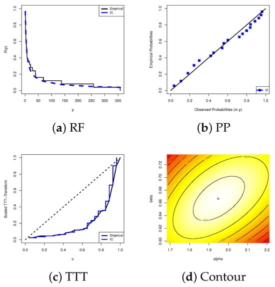
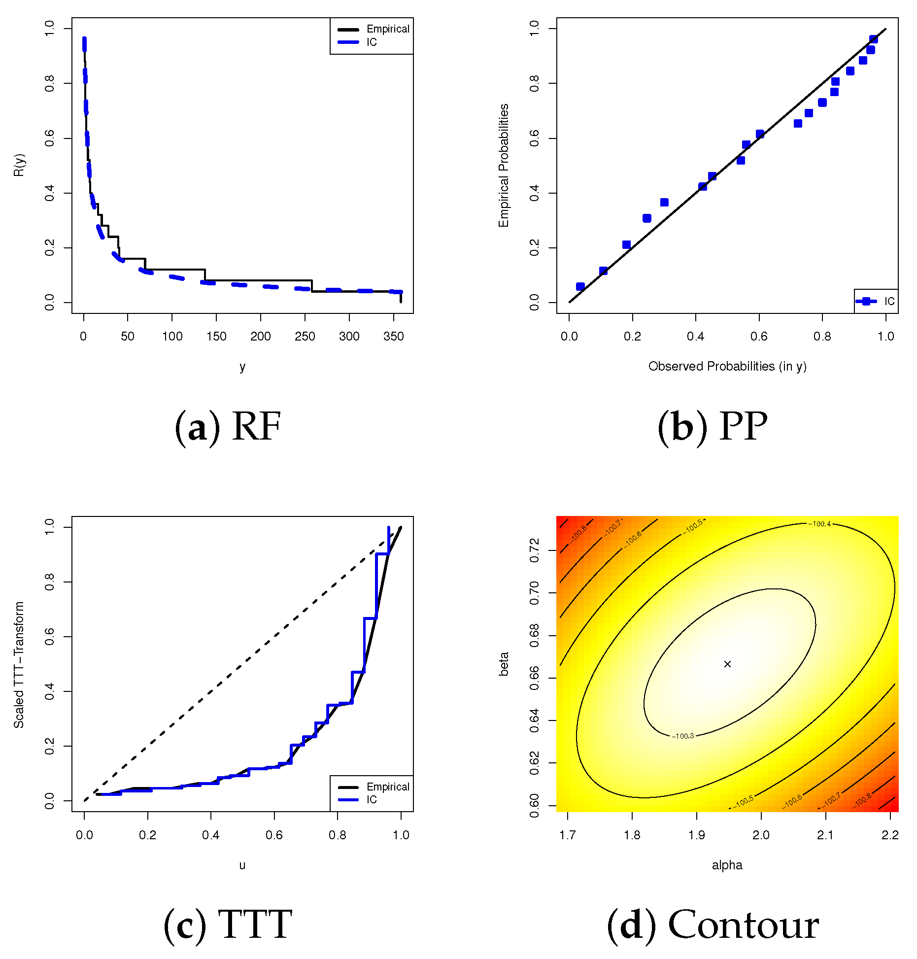
This finding confirms that the IC distribution provides an excellent fit for the given diamond data set. To further validate this conclusion, Figure 1 presents several graphical evaluations, including the following: (a) empirical/fitted RF curves; (b) empirical/fitted probability–probability (PP) lines; (c) empirical/fitted scaled-TTT plots; and (d) a contour for the log-likelihood IC parameters. A closer inspection of Figure 1a,b provides strong visual confirmation that the IC model effectively characterizes the survival behavior of diamond specimens, aligning well with the fitting results. Furthermore, Figure 1c highlights that the failure rate pattern of the observed data exhibits an increasing shape. Finally, Figure 1d reveals that the estimated parameters $\widehat{\alpha }\simeq 1.9479$ and $\widehat{\beta }\simeq 0.6665$, reinforcing the robustness of the estimation process. Consequently, we recommend utilizing these estimated values as initial parameter settings in subsequent computational applications to enhance both numerical efficiency and estimation accuracy.

Figure 1. Fitting diagrams for the IC model from diamond data.

To examine the utility of the proposed model, the IC distribution is compared with five other well-known distributions as competitors, see Table 6. To assess the validity of the IC model and its competitors, we used multiple goodness-of-fit measures, including (1) negative log-likelihood (N-logL), (2) Akaike information (A), (3) consistent Akaike information (CA), (4) Bayesian information (B), (5) Hannan–Quinn information (HQ), and (6) the Kolmogorov–Smirnov statistic with its p-value, see Table 7. The ML estimations of $\alpha$ and $\beta$ are used for calculating all fitted values for the given fit measures. Table 7 shows estimated parameters (along with their Std.Errs) and indicates that the IC distribution outperforms others due to it having the lowest fitting metrics except for the highest p-value.

Table 6. Five competitive models of the IC distribution.

Model	Symbol	Author(s)
Inverted Kumaraswamy	IK($\alpha ,\beta$)	Abd AL-Fattah et al. [32]
Inverted Lomax	IL($\alpha ,\beta$)	by Kleiber and Kotz [33]
Inverted exponentiated Pareto	IEP($\alpha ,\beta$)	by Abouammoh and Alshingiti [34]
Exponentiated inverted exponential	EIE($\alpha ,\beta$)	by Fatima and Ahmad [35]
Generalized inverted half-logistic	GIHL($\alpha ,\beta$)	by Potdar and Shirke [36]

Table 7. Fitting outputs of the IC model and its competitors from diamond data.

Model	$\mathit{\alpha }$		$\mathit{\beta }$		N-logL	A	CA	B	HQ	K-S (p-Value)
	Est.	Std.Err	Est.	Std.Err
IC	1.948	0.463	0.667	0.122	100.259	204.517	205.063	206.955	205.193	0.100(0.965)
IK	0.801	0.167	3.306	1.132	101.426	206.852	207.398	209.290	207.528	0.133(0.767)
IL	7.659	20.912	0.540	1.661	102.030	208.060	208.605	210.498	208.736	0.144(0.678)
IEP	0.743	0.183	3.721	1.048	101.289	206.578	207.123	209.015	207.254	0.132(0.777)
EIE	0.003	0.001	0.103	0.034	117.865	239.731	240.276	242.169	240.407	0.374(0.052)
GIHL	0.570	0.132	0.290	0.072	100.375	204.751	205.296	207.189	205.427	0.095(0.978)

We shall now use the full diamond data set reported to generate several APTIIC-BR samples with sizes $m(=10,20)$, based on different configurations of $\theta$ and $\tau$ (see Table 8). For each $\mathcal{S}i,i=1,2,3,5$, we computed the MLEs and 95% ACI estimates of $\alpha$, $\beta$, $R\left(y_0\right)$, $h\left(y_0\right)$ (at $y_0=5$), and $\theta$. Since prior information for the IC parameters ($\alpha$ and $\beta$) and binomial parameter $\theta$ is unavailable from the diamond data, by utilizing non-informative gamma priors, the Bayes point and 95% BCI estimates are developed through the suggested MCMC procedure, iterating $\mathcal{M}$ = 40,000 times, with the first 10,000 iterations discarded as burn-in.

Table 8. Different APTIIC-BR samples from diamond data.

Sample		$(\theta ,m)=(0.25,10)$ and $\{\tau \left(d\right),S^{\ast }\}=\{3.4\left(4\right),4\}$
$\mathcal{S}1$	i	1	2	3	4	5	6	7	8	9	10
	$s_i$	2	4	3	2	0	0	0	0	0	0
	$y_i$	1	1.5	2	3	4.5	7.5	9	16.5	20.5	40.5
		$(\theta ,m)=(0.75,10)$ and $\{\tau \left(d\right),S^{\ast }\}=\{4.0\left(2\right),1\}$
$\mathcal{S}2$	i	1	2	3	4	5	6	7	8	9	10
	$s_i$	11	3	0	0	0	0	0	0	0	0
	$y_i$	1	3	4.5	5	7	7.5	9	16.5	20.5	39
		$(\theta ,m)=(0.25,20)$ and $\{\tau \left(d\right),S^{\ast }\}=\{1.7\left(2\right),2\}$
$\mathcal{S}3$	i	1	2	3	4	5	6	7	8	9	10
	$s_i$	1	2	0	0	0	0	0	0	0	0
	$y_i$	1	1.5	2	2	2.5	3	3	4.5	5	7
	i	11	12	13	14	15	16	17	18	19	20
	$s_i$	0	0	0	0	0	0	0	0	0	0
	$y_i$	7	7.5	9	16.5	20.5	28	39	40.5	69.5	137
		$(\theta ,m)=(0.75,20)$ and $\{\tau \left(d\right),S^{\ast }\}=\{1.2\left(1\right),1\}$
$\mathcal{S}4$	i	1	2	3	4	5	6	7	8	9	10
	$s_i$	4	0	0	0	0	0	0	0	0	0
	$y_i$	1	1.5	2	2	2	2.5	3	4.5	5	7
	i	11	12	13	14	15	16	17	18	19	20
	$s_i$	0	0	0	0	0	0	0	0	0	0
	$y_i$	7.5	9	16.5	20.5	28	39	40.5	69.5	137	257.5

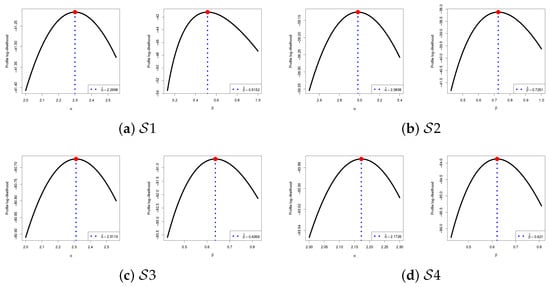
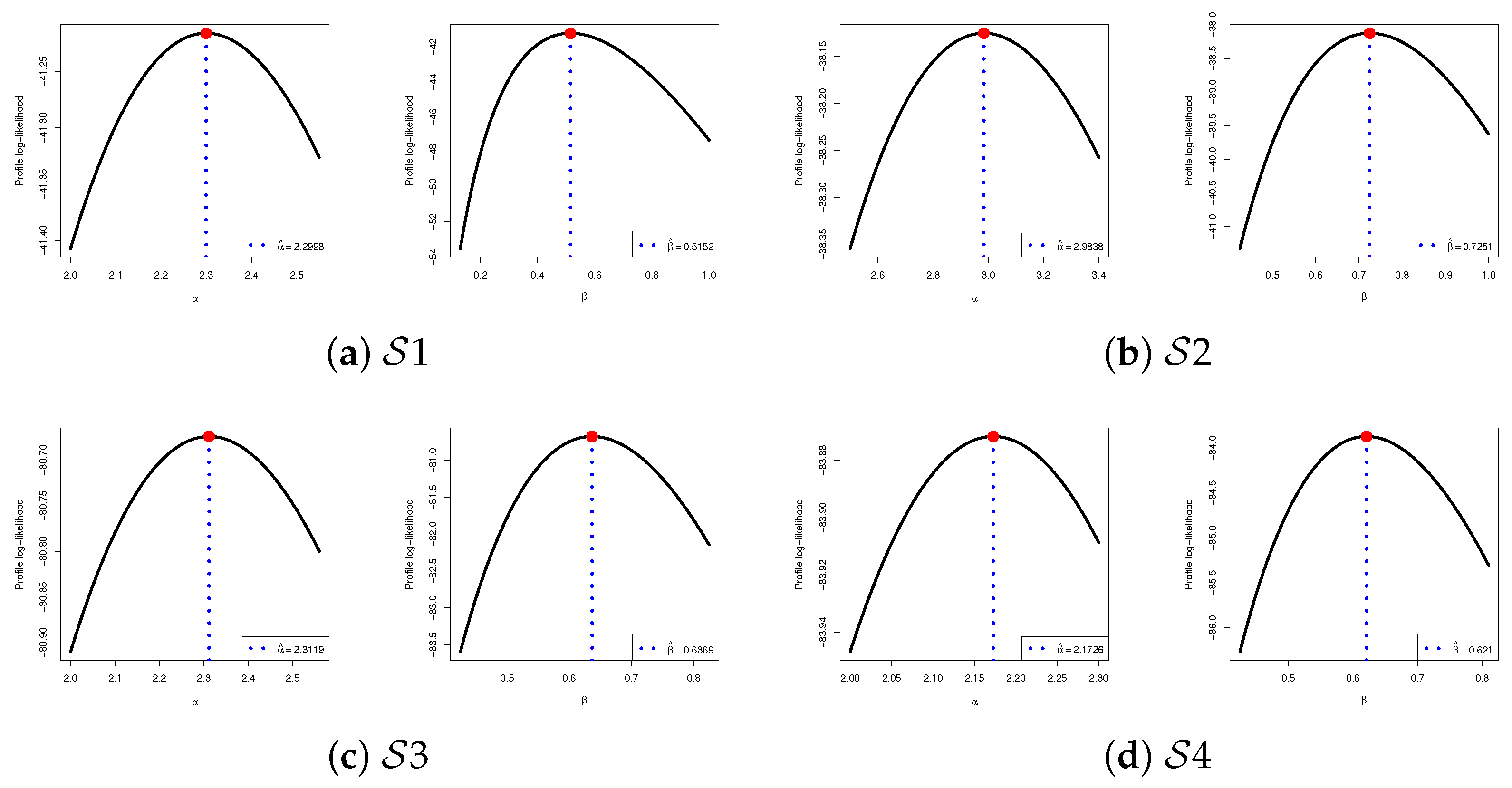
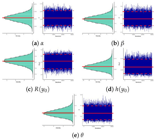
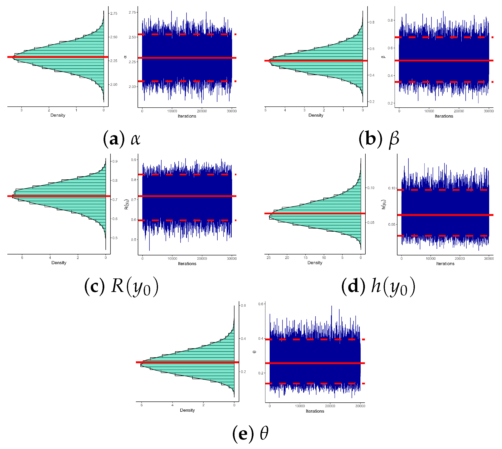
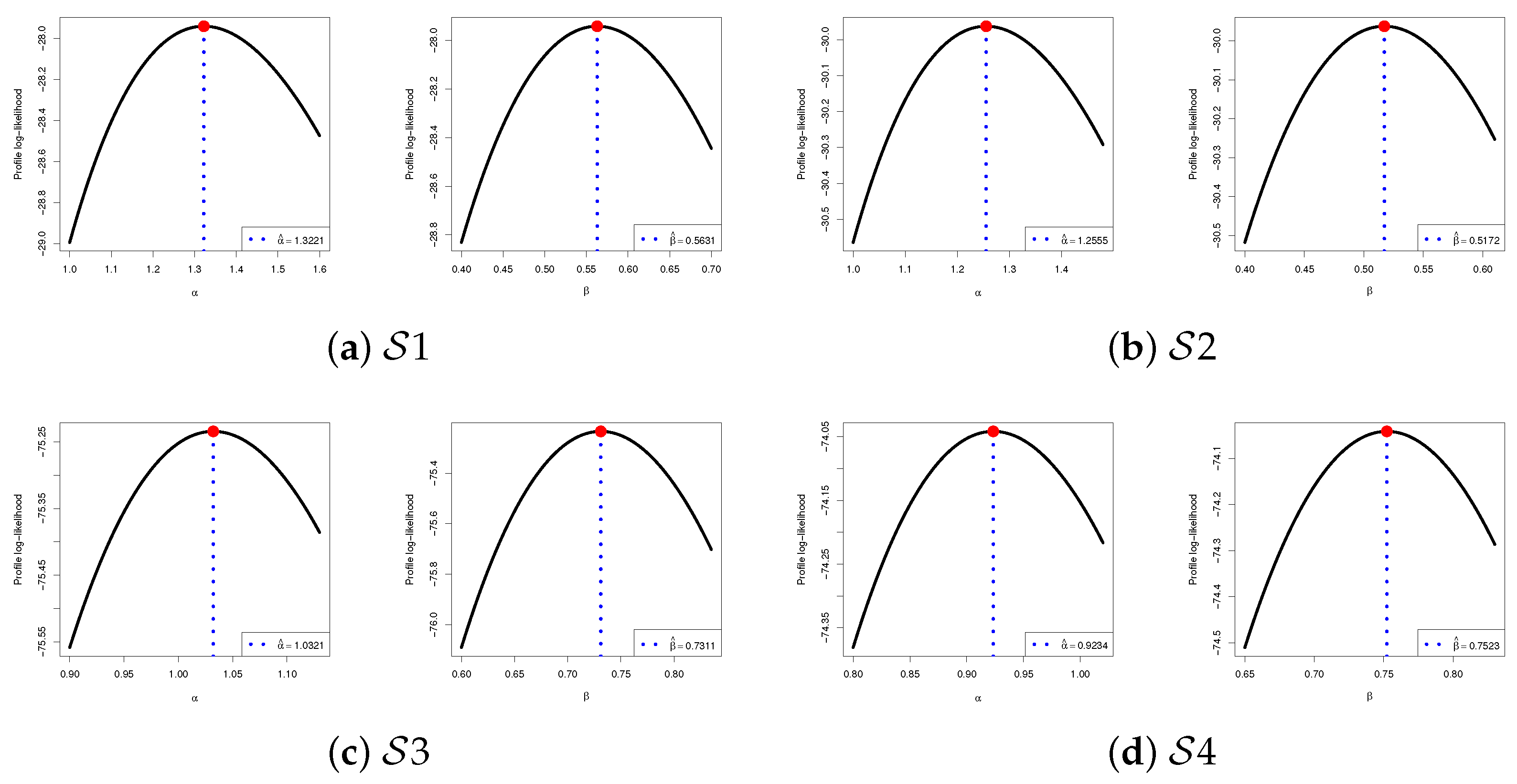
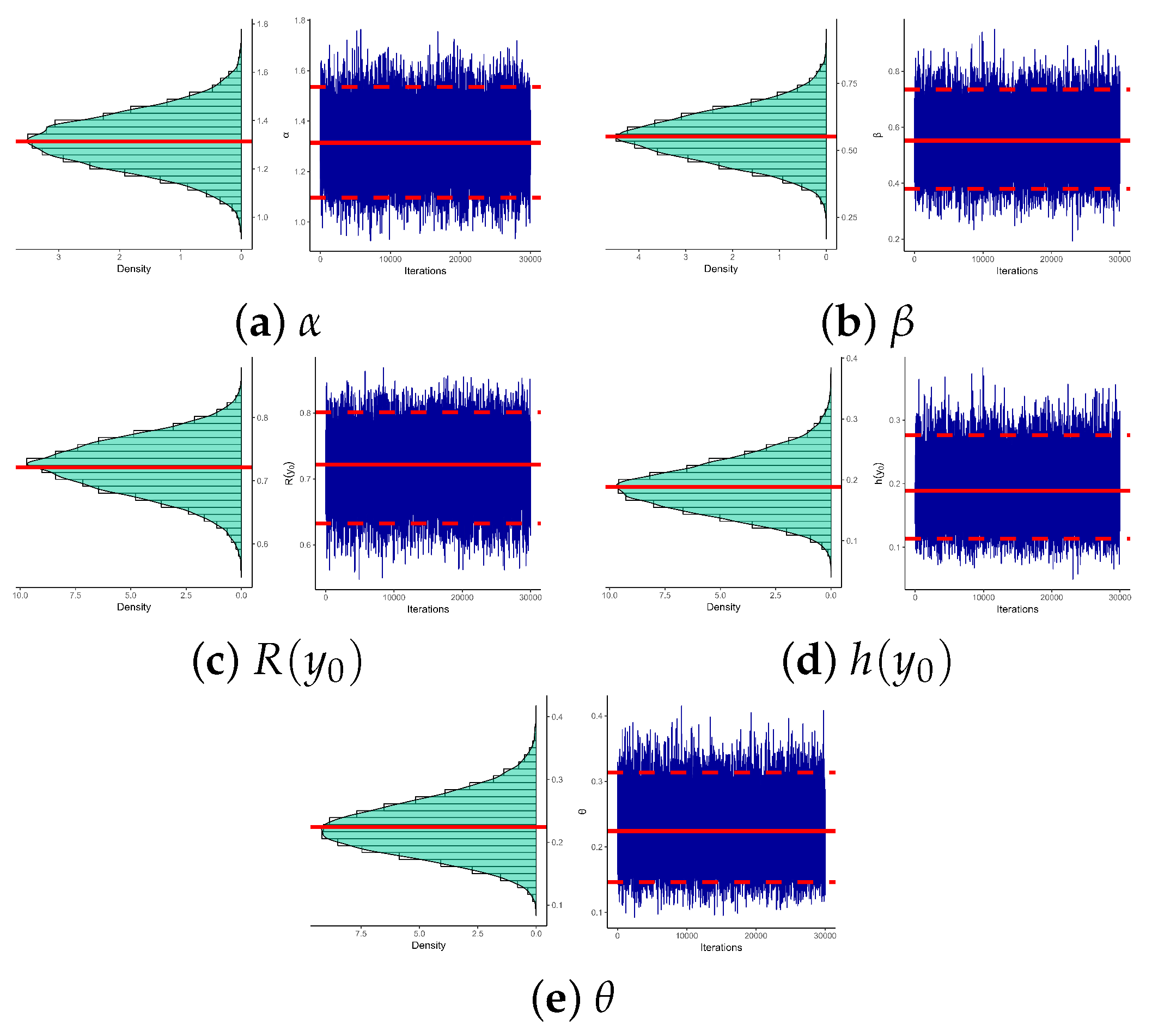
As a result, Table 9 presents both point estimates (with their Std.Errs) and interval estimates (with their interval lengths (ILs)) for each parameter. From Table 9, in terms of minimum Std.Err values, it is evident that the Bayesian MCMC estimates outperform those developed from the likelihood approach. This trend is also reflected in the BCIs when compared to the ACIs in terms of minimum IL values. Figure 2 presents the profile log-likelihood functions for the IC parameters $\alpha$ and $\beta$, constructed using $\mathcal{S}i,i=1,2,3,4,$ listed in Table 8. The subplots in Figure 2 provide strong evidence of both the existence and uniqueness of the fitted frequentist estimates $\widehat{\alpha }$ and $\widehat{\beta }$ of $\alpha$ and $\beta$, respectively. These results further substantiate the accuracy and reliability of the estimated values reported in Table 9, reinforcing the validity of the model fitting. To evaluate the convergence of the MCMC chains for $\alpha$, $\beta$, $R\left(y_0\right)$, $h\left(y_0\right)$, and $\theta$, Gaussian kernel density and trace plots for the remaining 30,000 MCMC iterations are generated from $\mathcal{S}1$ (as an example), as shown in Figure 3. The sub-plots in Figure 3 confirm satisfactory convergence of the MCMC process. They also indicate that the simulated posterior iterations of $\alpha$ are nearly symmetrical, while those of $R\left(y_0\right)$ are negatively skewed, whereas those for $\beta$, $h\left(y_0\right)$, and $\theta$ exhibit positive skewness.

Table 9. The point and interval estimates of $\alpha$, $\beta$, $R\left(y_0\right)$, $h\left(y_0\right)$, and $\theta$ from diamond data.

Sample	Par.	MLE		Bayes		ACI			BCI
		Est.	Std.Err	Est.	Std.Err	Low.	Upp.	IL	Low.	Upp.	IL
$\mathcal{S}1$	$\alpha$	2.30	0.64	2.29	0.12	1.04	3.56	2.51	2.05	2.53	0.47
	$\beta$	0.52	0.14	0.51	0.08	0.25	0.79	0.54	0.35	0.68	0.32
	$R\left(5\right)$	0.72	0.09	0.72	0.06	0.54	0.89	0.35	0.60	0.83	0.23
	$h\left(5\right)$	0.06	0.02	0.06	0.02	0.02	0.11	0.09	0.03	0.10	0.06
	$\theta$	0.26	0.07	0.26	0.07	0.13	0.39	0.26	0.14	0.39	0.26
$\mathcal{S}3$	$\alpha$	2.98	0.97	2.98	0.12	1.09	4.88	3.79	2.74	3.22	0.48
	$\beta$	0.73	0.18	0.72	0.09	0.38	1.07	0.70	0.54	0.91	0.37
	$R\left(5\right)$	0.66	0.11	0.67	0.06	0.46	0.87	0.42	0.54	0.79	0.25
	$h\left(5\right)$	0.09	0.03	0.09	0.02	0.03	0.15	0.12	0.06	0.13	0.08
	$\theta$	0.74	0.10	0.73	0.49	0.54	0.93	0.40	0.52	0.90	0.38
$\mathcal{S}4$	$\alpha$	2.31	0.61	2.30	0.12	1.12	3.51	2.39	2.06	2.54	0.48
	$\beta$	0.64	0.13	0.63	0.08	0.39	0.89	0.50	0.48	0.79	0.31
	$R\left(5\right)$	0.63	0.08	0.63	0.06	0.47	0.79	0.32	0.52	0.74	0.22
	$h\left(5\right)$	0.09	0.02	0.09	0.02	0.05	0.13	0.08	0.06	0.12	0.06
	$\theta$	0.33	0.16	0.34	0.17	0.03	0.64	0.62	0.09	0.65	0.56
$\mathcal{S}4$	$\alpha$	2.17	0.56	2.16	0.12	1.07	3.28	2.21	1.93	2.40	0.48
	$\beta$	0.62	0.12	0.62	0.08	0.38	0.86	0.49	0.47	0.77	0.31
	$R\left(5\right)$	0.62	0.08	0.62	0.06	0.45	0.79	0.33	0.51	0.73	0.22
	$h\left(5\right)$	0.09	0.02	0.09	0.02	0.05	0.13	0.09	0.06	0.12	0.06
	$\theta$	0.80	0.18	0.79	0.17	0.45	0.99	0.54	0.39	0.99	0.60

Figure 2. Profile log-likelihood curves of $\alpha$ (left) and $\beta$ (right) from diamond data.

Figure 3. The density and trace plots of $\alpha$, $\beta$, $R\left(y_0\right)$, $h\left(y_0\right)$, and $\theta$ from diamond data.

5.2. Airborne Communication Data

An airborne communication transceiver (ACT) is a high-frequency, bidirectional radio system designed to ensure seamless and reliable communication between aircraft and ground stations, enhancing aviation safety and operational efficiency. This application analyzes forty observations of the active repair times for an ACT. This data set has been reanalyzed by Elshahhat et al. [37]. However, the active repair times for the ACT are 0.50, 0.60, 0.60, 0.70, 0.70, 0.70, 0.80, 0.80, 1.00, 1.00, 1.00, 1.00, 1.10, 1.30, 1.50, 1.50, 1.50, 1.50, 2.00, 2.00, 2.20, 2.50, 2.70, 3.00, 3.00, 3.30, 4.00, 4.00, 4.50, 4.70, 5.00, 5.40, 5.40, 7.00, 7.50, 8.80, 9.00, 10.2, 22.0, and 24.5.

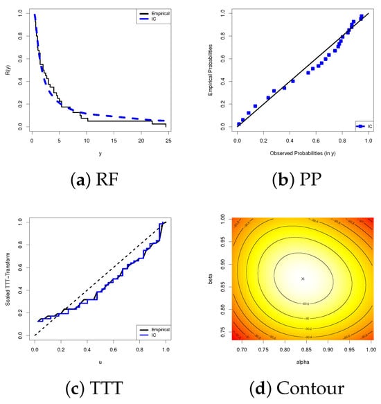
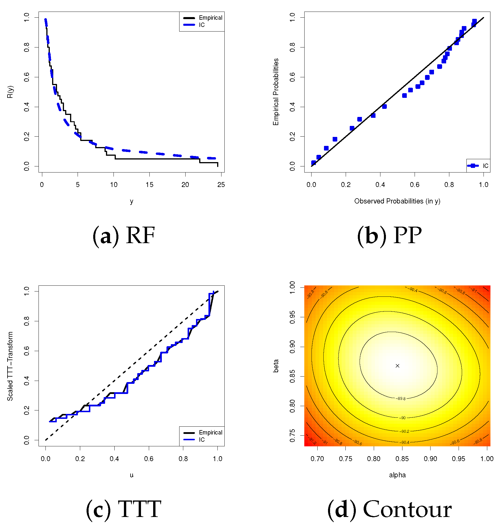
From the ACT data, we obtain the KS (p-value) as 0.0982 (0.8356). These findings confirm that the IC distribution provides an excellent fit for the ACT data set. To further validate this conclusion, Figure 4 presents multiple graphical assessments; a detailed analysis of Figure 4a,b visually supports the adequacy of the IC model in describing the data set, complementing the numerical fitting results. Additionally, Figure 4c reveals an upside-down bathtub failure rate, while Figure 4d highlights the fitted values $\widehat{\alpha }\approx 0.8417$ and $\widehat{\beta }\approx 0.8679$, confirming the stability of the estimation process. Again, to improve both numerical stability and estimation precision, we recommend using these parameter estimates as initial values for future computational analyses.

Figure 4. Fitting diagrams for the IC model from ACT data.

Again, using the same comparison scenarios discussed earlier in Section 5.1, we now highlight the superiority of the IC distribution compared to its competitors reported in Table 6. As a result, Table 10 reveals that the IC distribution surpasses others by having the lowest fitting metrics except for the greatest p-value.

Table 10. Fitting outputs of the IC model and its competitors from ACT data.

Model	$\mathit{\alpha }$		$\mathit{\beta }$		N-logL	A	CA	B	HQ	K-S (p-Value)
	Est.	Std.Err	Est.	Std.Err
IC	0.842	0.134	0.868	0.111	89.669	183.338	183.662	186.716	184.559	0.098 (0.836)
IK	1.662	0.262	4.333	1.237	90.313	184.627	184.951	188.005	185.848	0.107(0.747)
IL	28.36	61.69	0.056	0.125	90.731	185.463	185.787	188.840	186.684	0.101(0.832)
IEP	1.913	0.442	3.230	0.566	90.616	185.232	185.556	188.609	186.453	0.115(0.665)
EIE	0.279	0.149	0.995	0.458	93.122	190.243	190.568	193.621	191.464	0.194(0.100)
GIHL	1.047	0.212	0.460	0.077	89.887	183.774	184.099	187.152	184.996	0.101(0.811)

Utilizing all the ACT data, four distinct APTIIC-BR samples are generated, see Table 11. For each sample in $\mathcal{S}i,i=1,2,3,4$, both frequentist and Bayesian estimates (with their Std.Errs) of $\alpha$, $\beta$, $R\left(y_0\right)$, $h\left(y_0\right)$ (at $y_0=2$), and $\theta$ are computed, see Table 12. Additionally, in Table 12, the 95% ACI/BCI bounds (with their ILs) of $\alpha$, $\beta$, $R\left(y_0\right)$, $h\left(y_0\right)$ (at $y_0=2$), and $\theta$ are reported. All Bayes calculations developed from ACT data are implemented using the same scenarios discussed previously in Section 5.1.

Table 11. Different APTIIC-BR samples from ACT data.

Sample		$(\theta ,m)=(0.25,10)$ and $\{\tau \left(d\right),S^{\ast }\}=\{1.75\left(5\right),9\}$
$\mathcal{S}1$	i	1	2	3	4	5	6	7	8	9	10
	$s_i$	5	8	6	0	2	0	0	0	0	0
	$y_i$	0.50	0.70	0.80	1.10	1.30	2.00	2.20	2.50	3.30	4.70
		$(\theta ,m)=(0.75,10)$ and $\{\tau \left(d\right),S^{\ast }\}=\{0.55\left(1\right),7\}$
$\mathcal{S}2$	i	1	2	3	4	5	6	7	8	9	10
	$s_i$	23	0	0	0	0	0	0	0	0	0
	$y_i$	0.50	0.60	0.80	1.30	2.00	2.50	3.00	4.50	5.40	7.00
		$(\theta ,m)=(0.25,30)$ and $\{\tau \left(d\right),S^{\ast }\}=\{0.65\left(3\right),4\}$
$\mathcal{S}3$	i	1	2	3	4	5	6	7	8	9	10
	$s_i$	3	0	3	0	0	0	0	0	0	0
	$y_i$	0.50	0.60	0.60	0.70	0.80	1.00	1.00	1.10	1.30	1.50
	i	11	12	13	14	15	16	17	18	19	20
	$s_i$	0	0	0	0	0	0	0	0	0	0
	$y_i$	1.50	2.00	2.00	2.20	2.50	2.70	3.00	3.00	3.30	4.00
	i	21	22	23	24	25	26	27	28	29	30
	$s_i$	0	0	0	0	0	0	0	0	0	0
	$y_i$	4.00	4.50	4.70	5.00	5.40	7.00	7.50	8.80	9.00	10.2
		$(\theta ,m)=(0.75,30)$ and $\{\tau \left(d\right),S^{\ast }\}=\{0.55\left(1\right),2\}$
$\mathcal{S}4$	i	1	2	3	4	5	6	7	8	9	10
	$s_i$	8	0	0	0	0	0	0	0	0	0
	$y_i$	0.50	0.60	0.60	0.70	0.70	0.80	1.00	1.00	1.10	1.30
	i	11	12	13	14	15	16	17	18	19	20
	$s_i$	0	0	0	0	0	0	0	0	0	0
	$y_i$	1.50	1.50	1.50	2.00	2.20	2.50	2.70	3.00	3.30	4.00
	i	21	22	23	24	25	26	27	28	29	30
	$s_i$	0	0	0	0	0	0	0	0	0	0
	$y_i$	4.50	4.70	5.00	5.40	7.00	7.50	8.80	9.00	10.2	22.0

Table 12. The point and interval estimates of $\alpha$, $\beta$, $R\left(y_0\right)$, $h\left(y_0\right)$, and $\theta$ from ACT data.

Sample	Par.	MLE		Bayes		ACI			BCI
		Est.	Std.Err	Est.	Std.Err	Low.	Upp.	IL	Low.	Upp.	IL
$\mathcal{S}1$	$\alpha$	1.32	0.25	1.31	0.11	0.84	1.81	0.97	1.10	1.54	0.44
	$\beta$	0.56	0.13	0.55	0.09	0.31	0.82	0.51	0.38	0.74	0.36
	$R\left(2\right)$	0.72	0.08	0.72	0.04	0.56	0.88	0.32	0.63	0.80	0.17
	$h\left(2\right)$	0.19	0.06	0.19	0.04	0.07	0.32	0.25	0.11	0.28	0.16
	$\theta$	0.22	0.04	0.22	0.05	0.14	0.31	0.17	0.15	0.31	0.17
$\mathcal{S}2$	$\alpha$	1.26	0.26	1.25	0.11	0.75	1.76	1.01	1.03	1.47	0.44
	$\beta$	0.52	0.12	0.51	0.09	0.29	0.75	0.46	0.34	0.68	0.34
	$R\left(2\right)$	0.72	0.09	0.72	0.04	0.55	0.89	0.34	0.63	0.80	0.17
	$h\left(2\right)$	0.18	0.06	0.18	0.04	0.06	0.30	0.24	0.10	0.26	0.15
	$\theta$	0.77	0.08	0.76	0.08	0.62	0.92	0.30	0.60	0.89	0.29
$\mathcal{S}3$	$\alpha$	1.03	0.17	1.03	0.10	0.69	1.37	0.67	0.83	1.22	0.40
	$\beta$	0.73	0.10	0.73	0.08	0.53	0.94	0.41	0.57	0.88	0.31
	$R\left(2\right)$	0.57	0.07	0.57	0.04	0.44	0.71	0.28	0.48	0.66	0.17
	$h\left(2\right)$	0.31	0.06	0.31	0.04	0.19	0.42	0.23	0.23	0.39	0.17
	$\theta$	0.25	0.09	0.25	0.09	0.08	0.42	0.35	0.10	0.44	0.33
$\mathcal{S}4$	$\alpha$	0.92	0.16	0.92	0.10	0.61	1.23	0.62	0.73	1.11	0.38
	$\beta$	0.75	0.11	0.75	0.08	0.54	0.97	0.43	0.59	0.91	0.32
	$R\left(2\right)$	0.53	0.07	0.53	0.05	0.38	0.67	0.29	0.43	0.62	0.18
	$h\left(2\right)$	0.34	0.06	0.33	0.05	0.21	0.46	0.25	0.25	0.43	0.18
	$\theta$	0.80	0.13	0.79	0.13	0.55	1.05	0.50	0.52	0.97	0.45

The results in Table 12 indicate that Bayesian point and credible interval estimates of $\alpha$, $\beta$, $R\left(y_0\right)$, $h\left(y_0\right)$, and $\theta$ consistently exhibit superior statistical properties in terms of minimum Std. Err. and IL values compared to those obtained via the likelihood approach.

For $\mathcal{S}i,i=1,2,3,4,$ presented in Table 11, Figure 5 shows that estimates of $\widehat{\alpha }$ and $\widehat{\beta }$ (reported in Table 12) exist and are unique. Additionally, Figure 6 illustrates density histograms (with MCMC realizations) and trace plots for 40,000 MCMC samples corresponding to $\alpha$, $\beta$, $R\left(y_0\right)$, $h\left(y_0\right)$, and $\theta$. The graphical diagnostics confirm that the MCMC algorithm achieves satisfactory convergence. Furthermore, the posterior distributions of $\alpha$ and $\beta$ appear approximately symmetric, while those of $R\left(y_0\right)$ display negative skewness, whereas those of $h\left(y_0\right)$ and $\theta$ display positive skewness.

Figure 5. Profile log-likelihood curves of $\alpha$ (left) and $\beta$ (right) from ACT data.

Figure 6. The density and trace plots of $\alpha$, $\beta$, $R\left(y_0\right)$, $h\left(y_0\right)$, and $\theta$ from ACT data.

The empirical analysis of the two data sets demonstrates that the IC lifetime distribution provides a good fit for data collected under the proposed censoring scheme. Moreover, the results highlight the advantages of the Bayesian MCMC approach, which delivers more accurate and efficient parameter estimates when handling such censored data.

6. Concluding Remarks

This study emphasized the value of the adaptive progressive Type-II censoring scheme with binomial removals as a flexible and useful strategy for data collection, offering significant advantages over traditional fixed removal patterns. Recognizing the critical role of the inverse Chen distribution in modeling real-world phenomena characterized by diverse failure rate behaviors, such as increasing, decreasing, and upside-down bathtub-shaped patterns, we addressed the estimation challenges associated with its parameters, the binomial distribution parameter, and two essential reliability metrics: the reliability and hazard rate functions. By examining both classical and Bayesian estimation techniques, we provided comprehensive solutions for both point and interval estimations, offering insights into the inverse Chen distribution’s reliability characteristics. Classical estimation was carried out using the maximum likelihood method, with approximate confidence intervals calculated based on the asymptotic properties of the estimates. In the Bayesian approach, the squared error loss function was applied, and Markov Chain Monte Carlo methods were used to obtain Bayes estimates and create symmetric Bayesian credible intervals. The effectiveness of these methods was thoroughly assessed through an extensive simulation study, which confirmed their accuracy and efficiency. Monte Carlo simulation outcomes indicated that the Markovian iterations for all unknown subjects produce more accurate results compared to the classical estimates. Ultimately, the application results align with the simulation findings, demonstrating the practical adaptability of the proposed estimation methodologies in real-world engineering reliability studies. One important limitation of the current study is that the adaptive progressive Type-II censoring plan with binomial removals is most effective when the total duration of the experiment is not a primary concern. In situations involving highly reliable products, where failures are infrequent and testing time may become extreme, alternative censoring strategies, such as an improved version of the adaptive progressive Type-II censoring plan with binomial removals, may be more appropriate. Accordingly, a promising direction for future research is to investigate the reliability analysis of the inverse Chen distribution under an improved adaptive progressive Type-II censoring plan with binomial removals. Another key direction for future research involves integrating advanced deep learning methodologies such as ensemble techniques to improve the prediction of reliability metrics, see for more detail Xu et al. [38].

References

- Chen, Z. A new two-parameter lifetime distribution with bathtub shape or increasing failure rate function. Stat. Probab. Lett. 2000, 49, 155–161. [Google Scholar] [CrossRef] [Scilit]
- Zamani, Z.; Afshari, M.; Karamikabir, H.; Ahmadi, M.K.; Alizadeh, M. The new extension of odd log-logistic chen distribution: Mathematical properties and applications. Thail. Stat. 2021, 19, 317–338. [Google Scholar]
- Zamani, Z.; Afshari, M.; Karamikabir, H.; Alizadeh, M.; Ali, M.M. Extended exponentiated chen distribution: Mathematical properties and applications. Stat. Optim. Inf. Comput. 2022, 10, 606–626. [Google Scholar] [CrossRef] [Scilit]
- Tarvirdizade, B.; Ahmadpour, M. A new extension of Chen distribution with applications to lifetime data. Commun. Math. Stat. 2021, 9, 23–38. [Google Scholar] [CrossRef] [Scilit]
- Srivastava, P.K.; Srivastava, R.S. Two parameter inverse Chen distribution as survival model. Int. J. Stat. Math. 2014, 11, 12–16. [Google Scholar]
- Agiwal, V. Bayesian estimation of stress strength reliability from inverse Chen distribution with application on failure time data. Ann. Data Sci. 2023, 10, 317–347. [Google Scholar] [CrossRef] [Scilit]
- Alotaibi, R.; Nassar, M.; Khan, Z.A.; Elshahhat, A. Statistical analysis of stress–strength in a newly inverted Chen model from adaptive progressive type-II censoring and modelling on light-emitting diodes and pump motors. AIMS Math. 2024, 9, 34311–34355. [Google Scholar] [CrossRef] [Scilit]
- Kumar, S.; Kumari, A.; Kumar, K. Bayesian and classical inferences in two inverse Chen populations based on joint Type-II censoring. Am. J. Theor. Appl. Stat. 2022, 11, 150–159. [Google Scholar]
- Balakrishnan, N. Progressive censoring methodology: An appraisal. Test 2007, 16, 211–259. [Google Scholar] [CrossRef] [Scilit]
- Kundu, D. Bayesian inference and life testing plan for the Weibull distribution in presence of progressive censoring. Technometrics 2008, 50, 144–154. [Google Scholar] [CrossRef] [Scilit]
- Ng, H.K.T.; Luo, L.; Hu, Y.; Duan, F. Parameter estimation of three-parameter Weibull distribution based on progressively type-II censored samples. J. Stat. Comput. Simul. 2012, 82, 1661–1678. [Google Scholar] [CrossRef] [Scilit]
- Ghanbari, S.; Rezaei Roknabadi, A.; Salehi, M. Estimation of stress–strength reliability for Marshall–Olkin distributions based on progressively Type-II censored samples. J. Appl. Stat. 2022, 49, 1913–1934. [Google Scholar] [CrossRef] [Scilit]
- AL-Zaydi, A.M. On Moments of Inverse Kumaraswamy Distribution Based on Progressive Type-II Censored Order Statistics. J. Stat. Theory Appl. 2024, 23, 500–524. [Google Scholar] [CrossRef] [Scilit]
- Ng, H.K.T.; Kundu, D.; Chan, P.S. Statistical analysis of exponential lifetimes under an adaptive Type-II progressive censoring scheme. Nav. Res. Logist. 2009, 56, 687–698. [Google Scholar] [CrossRef] [Scilit]
- Panahi, H.; Moradi, N. Estimation of the inverted exponentiated Rayleigh distribution based on adaptive Type II progressive hybrid censored sample. J. Comput. Appl. Math. 2020, 364, 112345. [Google Scholar] [CrossRef] [Scilit]
- Kohansal, A.; Shoaee, S. Bayesian and classical estimation of reliability in a multicomponent stress-strength model under adaptive hybrid progressive censored data. Stat. Pap. 2021, 62, 309–359. [Google Scholar] [CrossRef] [Scilit]
- Helu, A. Inference on overlapping coefficient in two exponential populations based on adaptive type-II progressive hybrid censoring. Afr. Mat. 2025, 36, 9. [Google Scholar] [CrossRef] [Scilit]
- Sharma, H.; Kumar, P. On survival estimation of Lomax distribution under adaptive progressive type-II censoring. Stat. Transit. New Ser. 2025, 26, 51–67. [Google Scholar] [CrossRef] [Scilit]
- Kumari, R.; Sultana, F.; Tripathi, Y.M.; Sinha, R.K. Parametric inference for inverted exponentiated family with jointly adaptive progressive type-II censoring. Life Cycle Reliab. Saf. Eng. 2025, 14, 37–56. [Google Scholar] [CrossRef] [Scilit]
- Yuen, H.K.; Tse, S.K. Parameters estimation for Weibull distributed lifetimes under progressive censoring with random removals. J. Stat. Comput. Simul. 1996, 55, 57–71. [Google Scholar] [CrossRef] [Scilit]
- Tse, S.K.; Yang, C.; Yuen, H.K. Statistical analysis of Weibull distributed lifetime data under Type II progressive censoring with binomial removals. J. Appl. Stat. 2000, 27, 1033–1043. [Google Scholar] [CrossRef] [Scilit]
- Wu, S.J.; Chen, Y.J.; Chang, C.T. Statistical inference based on progressively censored samples with random removals from the Burr type XII distribution. J. Stat. Comput. Simul. 2007, 77, 19–27. [Google Scholar] [CrossRef] [Scilit]
- Elbatal, I.; Hassan, A.S.; Diab, L.S.; Ben Ghorbal, A.; Elgarhy, M.; El-Saeed, A.R. Stress–Strength Reliability Analysis for Different Distributions Using Progressive Type-II Censoring with Binomial Removal. Axioms 2023, 12, 1054. [Google Scholar] [CrossRef] [Scilit]
- Elshahhat, A.; Nassar, M. Analysis of adaptive Type-II progressively hybrid censoring with binomial removals. J. Stat. Comput. Simul. 2023, 93, 1077–1103. [Google Scholar] [CrossRef] [Scilit]
- Greene, W.H. Econometric Analysis, 4th ed.; Prentice-Hall: New York, NY, USA, 2000. [Google Scholar]
- Zhuang, L.; Xu, A.; Wang, Y.; Tang, Y. Remaining useful life prediction for two-phase degradation model based on reparameterized inverse Gaussian process. Eur. J. Oper. Res. 2024, 319, 877–890. [Google Scholar] [CrossRef] [Scilit]
- Al-Essa, L.A.; Soliman, A.A.; Abd-Elmougod, G.A.; Alshanbari, H.M. Adaptive type-II hybrid progressive censoring samples for statistical inference of comparative inverse Weibull distributions. Axioms 2023, 12, 973. [Google Scholar] [CrossRef] [Scilit]
- Soliman, A.A.; Abd Ellah, A.H.; Abou-Elheggag, N.A.; El-Sagheer, R.M. Inferences using type-II progressively censored data with binomial removals. Arab. J. Math. 2015, 4, 127–139. [Google Scholar] [CrossRef] [Scilit]
- Henningsen, A.; Toomet, O. maxLik: A package for maximum likelihood estimation in R. Comput. Stat. 2011, 26, 443–458. [Google Scholar] [CrossRef] [Scilit]
- Plummer, M.; Best, N.; Cowles, K.; Vines, K. coda: Convergence diagnosis and output analysis for MCMC. R News 2006, 6, 7–11. [Google Scholar]
- Alqasem, O.A.; Nassar, M.; Abd Elwahab, M.E.; Elshahhat, A. A new inverted Pham distribution for data modeling of mechanical components and diamond in South-West Africa. Phys. Scr. 2024, 99, 115268. [Google Scholar] [CrossRef] [Scilit]
- Abd AL-Fattah, A.M.; El-Helbawy, A.A.; Al-Dayian, G.R. Inverted Kumaraswamy distribution: Properties and estimation. Pak. J. Stat. 2017, 33, 37–61. [Google Scholar]
- Kleiber, C.; Kotz, S. Statistical Size Distributions in Economics and Actuarial Sciences; Wiley & Sons, Inc.: Hoboken, NJ, USA, 2003. [Google Scholar]
- Abouammoh, A.M.; Alshingiti, A.M. Reliability estimation of generalized inverted exponential distribution. J. Stat. Comput. Simulat. 2009, 79, 1301–1315. [Google Scholar] [CrossRef] [Scilit]
- Fatima, K.; Ahmad, S.P. The Exponentiated Inverted Exponential Distribution. J. Appl. Inf. Sci. 2017, 5, 35–41. [Google Scholar]
- Potdar, K.G.; Shirke, D.T. Inference for the parameters of generalized inverted family of distributions. ProbStat Forum 2013, 6, 18–28. [Google Scholar]
- Elshahhat, A.; El-Sherpieny, E.S.A.; Hassan, A.S. The Pareto–Poisson Distribution: Characteristics, Estimations and Engineering Applications. Sankhya A 2023, 85, 1058–1099. [Google Scholar] [CrossRef] [Scilit]
- Xu, A.; Wang, R.; Weng, X.; Wu, Q.; Zhuang, L. Strategic integration of adaptive sampling and ensemble techniques in federated learning for aircraft engine remaining useful life prediction. Appl. Soft Comput. 2025, 175, 113067. [Google Scholar] [CrossRef] [Scilit]
Disclaimer/Publisher’s Note: The statements, opinions and data contained in all publications are solely those of the individual author(s) and contributor(s) and not of MDPI and/or the editor(s). MDPI and/or the editor(s) disclaim responsibility for any injury to people or property resulting from any ideas, methods, instructions or products referred to in the content. |
© 2025 by the authors. Licensee MDPI, Basel, Switzerland. This article is an open access article distributed under the terms and conditions of the Creative Commons Attribution (CC BY) license (https://creativecommons.org/licenses/by/4.0/).