Similarity Solutions of Partial Differential–Integral Equations from the Theory of Stochastic Processes

Abstract

First-exit problems are studied for two-dimensional diffusion processes with jumps according to a Poisson process. The size of the jumps is distributed as an exponential random variable. We are interested in the random variable that denotes the first time that the sum of the two components of the process leaves a given interval. The function giving the probability that the process will leave the interval on its left-hand side satisfies a partial differential–integral equation. This equation is solved analytically in particular cases by making use of the method of similarity solutions. The problem of calculating the mean and the moment-generating function of the first-passage time random variable is also considered. The results obtained have applications in various fields, notably, financial mathematics and reliability theory.

1. Introduction

Let $\{B_i\left(t\right),t\ge 0\}$ be a one-dimensional standard Brownian motion starting at zero for $i=1,2$, and let $\left\{N\right(t),t\ge 0\}$ be a Poisson process with rate $\lambda$. The three stochastic processes are assumed to be independent. We define

$$\begin{array}{ccc}\hfill X\left(t\right)& =& X\left(0\right)+{\int }_0^t\rho [X\left(s\right),Y\left(s\right)]\mathrm{d}s+{\int }_0^t{\left\{v_1\left[X\left(s\right)\right]\right\}}^{1/2}\mathrm{d}{B}_1\left(s\right),\hfill \end{array}$$

(1)

$$\begin{array}{ccc}\hfill Y\left(t\right)& =& Y\left(0\right)+{\int }_0^{t}f\left[Y\left(s\right)\right]\mathrm{d}s+{\int }_0^t{\left\{v_2\left[Y\left(s\right)\right]\right\}}^{1/2}\mathrm{d}{B}_2\left(s\right)+\sum _{i=0}^{N\left(t\right)}{Z}_i,\hfill \end{array}$$

(2)

where $Z_1,Z_2,\dots$ are independent random variables that are distributed as the continuous random variable Z with the probability density function $f_Z\left(z\right)$ and are independent of the Poisson process. The functions $\rho (·,·)$, $f(·)$ and $v_i(·)\ge 0$, $i=1,2$, are such that $\left\{\right(X\left(t\right),Y\left(t\right)),t\ge 0\}$ is a two-dimensional jump-diffusion process.

If $v_1(·)\equiv 0$ and $\rho (·,·)$ is a non-negative or non-positive deterministic function, then $\left\{\right(X\left(t\right),Y\left(t\right)),t\ge 0\}$ could serve as a model for the wear or the remaining lifetime, respectively, of a device. The model would be a generalization of the one proposed by Rishel [1] and considered by Lefebvre in various papers (see, for instance, [2]).

Suppose that $\left(X\right(0),Y(0\left)\right)=(x,y)$, and let $\tau (x,y)$ be the first-exit time defined by

$$\tau (x,y)=inf\{t\ge 0:X\left(t\right)+Y\left(t\right)\notin (k_1,k_2)\mid k_1\le x+y\le k_2\}.$$

(3)

Generalizing the results in [3,4] (see also [5]), we can state that the moment-generating function

$$M(x,y)(=M(x,y;\alpha )):=E\left[e^{-\alpha \tau (x,y)}\right]$$

(4)

of $\tau (x,y)$, where $\alpha >0$, satisfies the partial differential–integral equation (PDIE)

$$\begin{array}{ccc}\hfill \alpha M(x,y)& =& \rho (x,y)M_x(x,y)+f\left(y\right)M_y(x,y)+{\displaystyle \frac{1}{2}}{v}_1\left(x\right)M_{xx}(x,y)+{\displaystyle \frac{1}{2}}{v}_2\left(y\right)M_{yy}(x,y)\hfill \\ & & +\lambda \left\{{\int }_{-\infty }^{\infty }M(x,y+z)f_Z\left(z\right)\mathrm{d}z-M(x,y)\right\}.\hfill \end{array}$$

(5)

In this paper, we assume that Z has an exponential distribution with parameter $\theta$. It follows that Equation (5) becomes

$$\begin{array}{ccc}\hfill \alpha M(x,y)& =& \rho (x,y)M_x(x,y)+f\left(y\right)M_y(x,y)+{\displaystyle \frac{1}{2}}{v}_1\left(x\right)M_{xx}(x,y)+{\displaystyle \frac{1}{2}}{v}_2\left(y\right)M_{yy}(x,y)\hfill \\ & & +\lambda \left\{{\int }_0^{\infty }M(x,y+z)\theta e^{-\theta z}\mathrm{d}z-M(x,y)\right\}.\hfill \end{array}$$

(6)

Since the jumps are positive, the boundary conditions are $M(x,y)=1$ if $x+y=k_1$ or $x+y\ge k_2$.

Similarly, the mean $m(x,y)$ of $\tau (x,y)$ satisfies the PDIE

$$\begin{array}{ccc}\hfill -1& =& \rho (x,y)m_x(x,y)+f\left(y\right)m_y(x,y)+{\displaystyle \frac{1}{2}}{v}_1\left(x\right)m_{xx}(x,y)+{\displaystyle \frac{1}{2}}{v}_2\left(y\right)m_{yy}(x,y)\hfill \\ & & +\lambda \left\{{\int }_0^{\infty }m(x,y+z)\theta e^{-\theta z}\mathrm{d}z-m(x,y)\right\}\hfill \end{array}$$

(7)

and is such that $m(x,y)=0$ if $x+y=k_1$ or $x+y\ge k_2$.

Finally, let

$$p(x,y)=P\left[X\left(\tau (x,y)\right)+Y\left(\tau (x,y)\right)=k_1\right].$$

(8)

This function, which is the probability of first exit at $k_1$, is a solution of the PDIE

$$\begin{array}{ccc}\hfill 0& =& \rho (x,y)p_x(x,y)+f\left(y\right)p_y(x,y)+{\displaystyle \frac{1}{2}}{v}_1\left(x\right)p_{xx}(x,y)+{\displaystyle \frac{1}{2}}{v}_2\left(y\right)p_{yy}(x,y)\hfill \\ & & +\lambda \left\{{\int }_0^{\infty }p(x,y+z)\theta e^{-\theta z}\mathrm{d}z-p(x,y)\right\}.\hfill \end{array}$$

(9)

The boundary conditions are $p(x,y)=1$ if $x+y=k_1$ and $p(x,y)=0$ if $x+y\ge k_2$.

In one dimension, and when there are no jumps, obtaining exact analytical expressions for the functions corresponding to $M(x,y)$, $m(x,y)$, and $p(x,y)$ is generally rather straightforward. When jumps are added to the model, the problem becomes much more difficult. Papers on problems of this type have been written by Abundo (see [6,7,8,9]). In [8], the first-passage area of one-dimensional jump-diffusion processes was computed. In addition to his papers on jump-diffusion processes, Lefebvre has also considered stochastic control problems for these processes. Jump-diffusion processes are especially important in financial mathematics; see the seminal paper by Merton [10], as well as [11]. Other papers on this subject are those by Cai [12], Peng and Liu [13], Yin et al. [14], Zhou and Wu [15], Gapeev and Stoev [16], Herrmann and Zucca [17], Song [18], and Ai et al. [19].

In the next section, we will compute the function $p(x,y)$ explicitly and exactly in three particular cases. First, taking advantage of the symmetry in the problems considered, we will make use of the method of similarity solutions to reduce Equation (9) to an integro-differential equation (IDE). Then, we will transform the IDE into an ordinary differential equation (ODE) of the third order. In Section 3, the problem of computing the mean $m(x,y)$ and the moment-generating function $M(x,y)$ of $\tau (x,y)$ will be studied. We will end this paper with a few remarks in Section 4.

2. Computation of the Probability $\mathit{p}(\mathit{x},\mathit{y})$

Case I. The first particular case that we consider is the following:

$$\begin{array}{ccc}\hfill X\left(t\right)& =& X\left(0\right)+c{\int }_0^{t}Y\left(s\right)\mathrm{d}s+{\int }_0^t\gamma \mathrm{d}{B}_1\left(s\right),\hfill \end{array}$$

(10)

$$\begin{array}{ccc}\hfill Y\left(t\right)& =& Y\left(0\right)-c{\int }_0^{t}Y\left(s\right)\mathrm{d}s+{\int }_0^t\sigma \mathrm{d}{B}_2\left(s\right)+\sum _{i=0}^{N\left(t\right)}{Z}_i,\hfill \end{array}$$

(11)

where c, $\gamma$, and $\sigma$ are positive constants. Then, $\left\{Y\right(t),t\ge 0\}$ is an Ornstein–Uhlenbeck process with Poissonian jumps. Moreover, if we let $\gamma$ decrease to zero, then $\left\{X\right(t),t\ge 0\}$ is an integrated Ornstein–Uhlenbeck process, which is multiplied by the constant c.

The PDIE (9) becomes

$$\begin{array}{ccc}\hfill 0& =& cy{p}_x(x,y)-cy{p}_y(x,y)+{\displaystyle \frac{1}{2}}{\gamma }^2{p}_{xx}(x,y)+{\displaystyle \frac{1}{2}}{\sigma }^2{p}_{yy}(x,y)\hfill \\ & & +\lambda \left\{{\int }_0^{\infty }p(x,y+z)\theta e^{-\theta z}\mathrm{d}z-p(x,y)\right\}.\hfill \end{array}$$

(12)

Now, based on the definition of the first-exit time $\tau (x,y)$, we will look for a solution of the form

$$p(x,y)=q\left(u\right),$$

(13)

where $u:=x+y$. This is an application of the method of similarity solutions to solve partial differential equations, and u is the similarity variable. For the method to work, we must be able to express (after simplification) all elements of Equation (12) in terms of u, as well as the boundary conditions. Here, the boundary conditions reduce to

$$q\left(k_1\right)=1\mathrm{and}q\left(u\right)=0\mathrm{if}u\ge k_2.$$

(14)

Furthermore, Equation (12) can be rewritten as follows:

$$\begin{array}{ccc}\hfill 0& =& {\displaystyle \frac{1}{2}}({\gamma }^2+{\sigma }^2)q^{\prime \prime }\left(u\right)+\lambda \left\{{\int }_0^{\infty }q(u+z)\theta e^{-\theta z}\mathrm{d}z-q\left(u\right)\right\}\hfill \\ & \stackrel{w:=u+z}{=}& {\displaystyle \frac{1}{2}}({\gamma }^2+{\sigma }^2)q^{\prime \prime }\left(u\right)+\lambda \left\{{\int }_u^{\infty }q\left(w\right)\theta e^{-\theta (w-u)}\mathrm{d}z-q\left(u\right)\right\}\hfill \\ & \stackrel{\mathrm{Equation}\left(14\right)}{=}& {\displaystyle \frac{1}{2}}({\gamma }^2+{\sigma }^2)q^{\prime \prime }\left(u\right)+\lambda \left\{{\int }_u^{k_2}q\left(w\right)\theta e^{-\theta (w-u)}\mathrm{d}z-q\left(u\right)\right\}.\hfill \end{array}$$

(15)

Next, differentiating the above equation with respect to u, we deduce from the Leibniz integral rule that

$$0={\displaystyle \frac{1}{2}}({\gamma }^2+{\sigma }^2)q^{\prime \prime \prime }\left(u\right)+\lambda \left\{-\theta q\left(u\right)+\theta {\int }_u^{k_2}q\left(w\right)\theta e^{-\theta (w-u)}\mathrm{d}z-q^{\prime }\left(u\right)\right\}.$$

(16)

Moreover, from Equation (15), we have

$$\lambda {\int }_u^{k_2}q\left(w\right)\theta e^{-\theta (w-u)}\mathrm{d}z=-{\displaystyle \frac{1}{2}}({\gamma }^2+{\sigma }^2)q^{\prime \prime }\left(u\right)+\lambda q\left(u\right).$$

(17)

Substituting this expression into Equation (16), we find that

$$0={\displaystyle \frac{1}{2}}({\gamma }^2+{\sigma }^2)q^{\prime \prime \prime }\left(u\right)-{\displaystyle \frac{\theta }{2}}({\gamma }^2+{\sigma }^2)q^{\prime \prime }\left(u\right)-\lambda q^{\prime }\left(u\right).$$

(18)

Notice that this is a second-order linear ODE with constant coefficients for $Q\left(u\right):=q^{\prime }\left(u\right)$. Its general solution is

$$q\left(u\right)={\mathit{c}}_{\mathit{1}}+{\mathit{c}}_{\mathit{2}}exp\left\{\left({\displaystyle \frac{{\theta }^2}{2}}+\kappa \right)u\right\}+{\mathit{c}}_{\mathit{3}}exp\left\{\left({\displaystyle \frac{{\theta }^2}{2}}-\kappa \right)u\right\},$$

(19)

where $c_i$ is an arbitrary constant for $i=1,2,3$, and

$$\kappa :={\displaystyle \frac{\sqrt{{\gamma }^4{\theta }^4+2{\gamma }^2{\sigma }^2{\theta }^4+{\sigma }^4{\theta }^4+8{\gamma }^2\lambda +8\lambda {\sigma }^2}}{2({\gamma }^2+{\sigma }^2)}}.$$

(20)

For the sake of simplicity, let us take $\gamma =\sigma =\lambda =\theta =1$, $k_1=0$, and $k_2=1$. Then,

$$q\left(u\right)={\mathit{c}}_{\mathit{1}}+{\mathit{c}}_{\mathit{2}}exp\left\{{\displaystyle \frac{\left(\sqrt{5}+1\right)u}{2}}\right\}+{\mathit{c}}_{\mathit{3}}exp\left\{{\displaystyle \frac{\left(1-\sqrt{5}\right)u}{2}}\right\}.$$

(21)

The unique solution of Equation (18) that satisfies the conditions $q\left(0\right)=1$, $q\left(1\right)=0$, and $q\left(0.5\right)=r$ is given by

$$\begin{array}{ccc}\hfill q\left(u\right)& =& {\displaystyle \frac{1}{\Delta }}[(r-1)exp\left\{{\displaystyle \frac{(1-u)\sqrt{5}}{2}}+{\displaystyle \frac{1}{2}}+{\displaystyle \frac{u}{2}}\right\}-exp\left\{{\displaystyle \frac{(2u-1)\sqrt{5}}{4}}+{\displaystyle \frac{u}{2}}+{\displaystyle \frac{1}{4}}\right\}\hfill \\ & & +exp\left\{{\displaystyle \frac{(1-2u)\sqrt{5}}{4}}+{\displaystyle \frac{u}{2}}+{\displaystyle \frac{1}{4}}\right\}+(1-r)exp\left\{{\displaystyle \frac{(u-1)\sqrt{5}}{2}}+{\displaystyle \frac{1}{2}}+{\displaystyle \frac{u}{2}}\right\}\hfill \\ & & -rexp\left\{-{\displaystyle \frac{(\sqrt{5}-1)u}{2}}\right\}+rexp\left\{{\displaystyle \frac{(\sqrt{5}+1)u}{2}}\right\}+rexp\left\{{\displaystyle \frac{1}{2}}-{\displaystyle \frac{\sqrt{5}}{2}}\right\}\hfill \\ & & -rexp\left\{{\displaystyle \frac{1}{2}}+{\displaystyle \frac{\sqrt{5}}{2}}\right\}-exp\left\{-{\displaystyle \frac{\sqrt{5}}{4}}+{\displaystyle \frac{3}{4}}\right\}+exp\left\{{\displaystyle \frac{\sqrt{5}}{4}}+{\displaystyle \frac{3}{4}}\right\}],\hfill \end{array}$$

(22)

where

$$\begin{array}{ccc}\hfill \Delta & :=& -exp\left\{-{\displaystyle \frac{\sqrt{5}}{4}}+{\displaystyle \frac{3}{4}}\right\}+exp\left\{{\displaystyle \frac{\sqrt{5}}{4}}+{\displaystyle \frac{3}{4}}\right\}+exp\left\{{\displaystyle \frac{\sqrt{5}}{4}}+{\displaystyle \frac{1}{4}}\right\}\hfill \\ & & -exp\left\{-{\displaystyle \frac{\sqrt{5}}{4}}+{\displaystyle \frac{1}{4}}\right\}-exp\left\{{\displaystyle \frac{1}{2}}+{\displaystyle \frac{\sqrt{5}}{2}}\right\}+exp\left\{{\displaystyle \frac{1}{2}}-{\displaystyle \frac{\sqrt{5}}{2}}\right\}.\hfill \end{array}$$

(23)

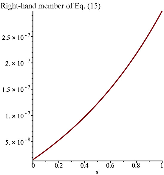
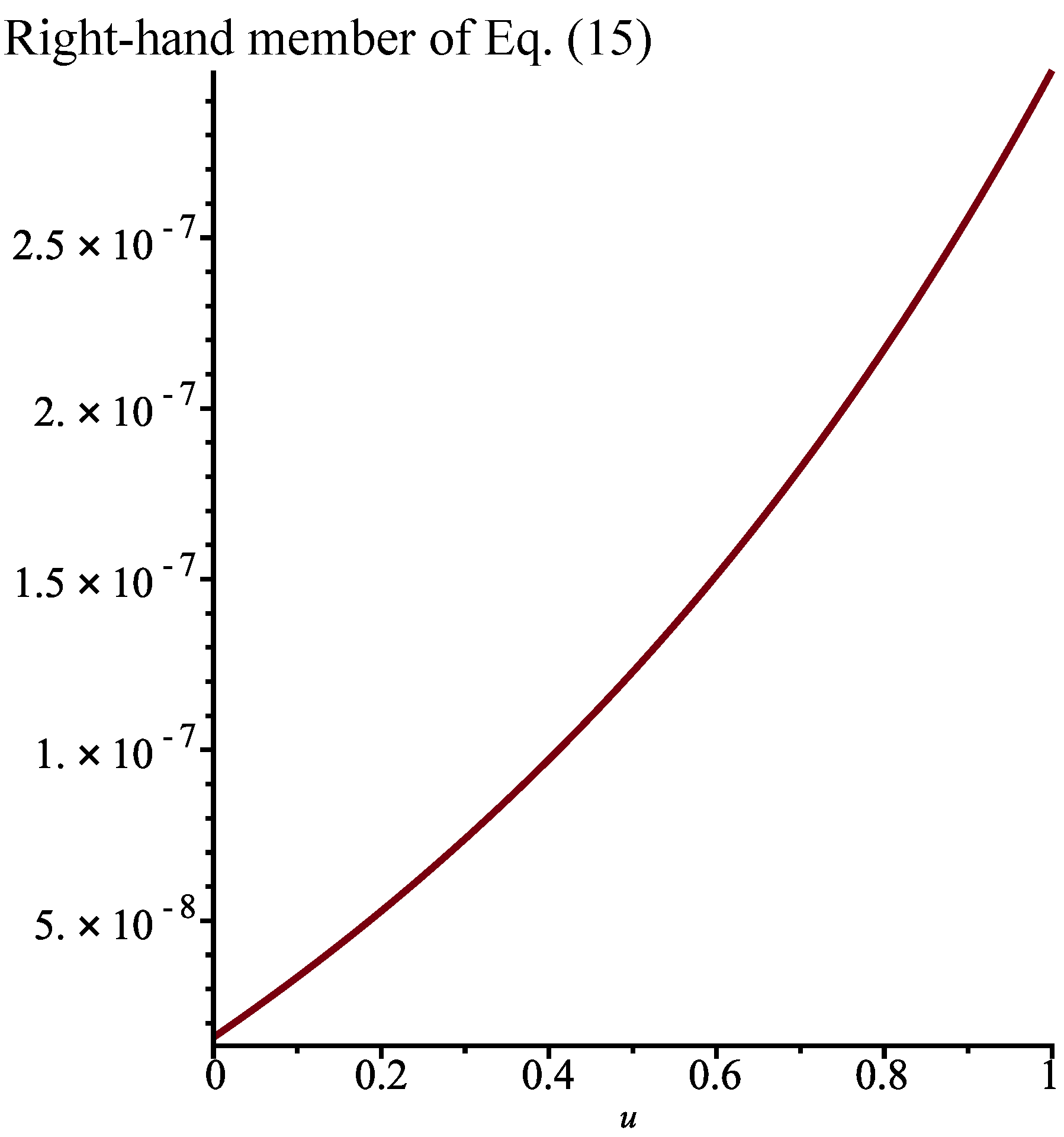
If we substitute the above function into Equation (15), we find that this equation is satisfied if we take $r\approx 0.4557$. Indeed, as can be seen in Figure 1, the right-hand member of Equation (15) is then practically equal to 0.

Figure 1. Right-hand member of Equation (15) for $u\in [0,1]$ with the function $q\left(u\right)$ defined in (22) and $r\approx 0.4557$ when $\gamma =\sigma =\lambda =\theta =1$, $k_1=0$, and $k_2=1$.

Proposition 1.

When $\gamma =\sigma =\lambda =\theta =1$, $k_1=0$, and $k_2=1$, the probability $p(x,y)$ is given by $q(x+y)$, where $q(·)$ is defined in Equation (22) and $r\approx 0.4557$. We have

$$p(x,y)\approx -0.8785-0.02976{\mathrm{e}}^{1.6180(x+y)}+1.9082{\mathrm{e}}^{-0.6180(x+y)}$$

(24)

for $0\le x+y\le 1$.

Remark 1.

We can calculate the function $p(x,y)$ for any admissible values of the parameters γ, σ, λ, and θ, as well as for any constants $k_1$ and $k_2$. However, the general solution is rather cumbersome. Moreover, to determine the value of the constant r, it is almost mandatory to choose particular values for all the quantities mentioned above.

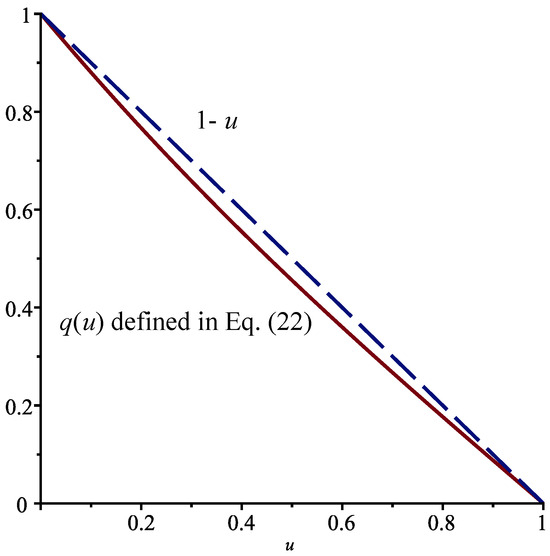
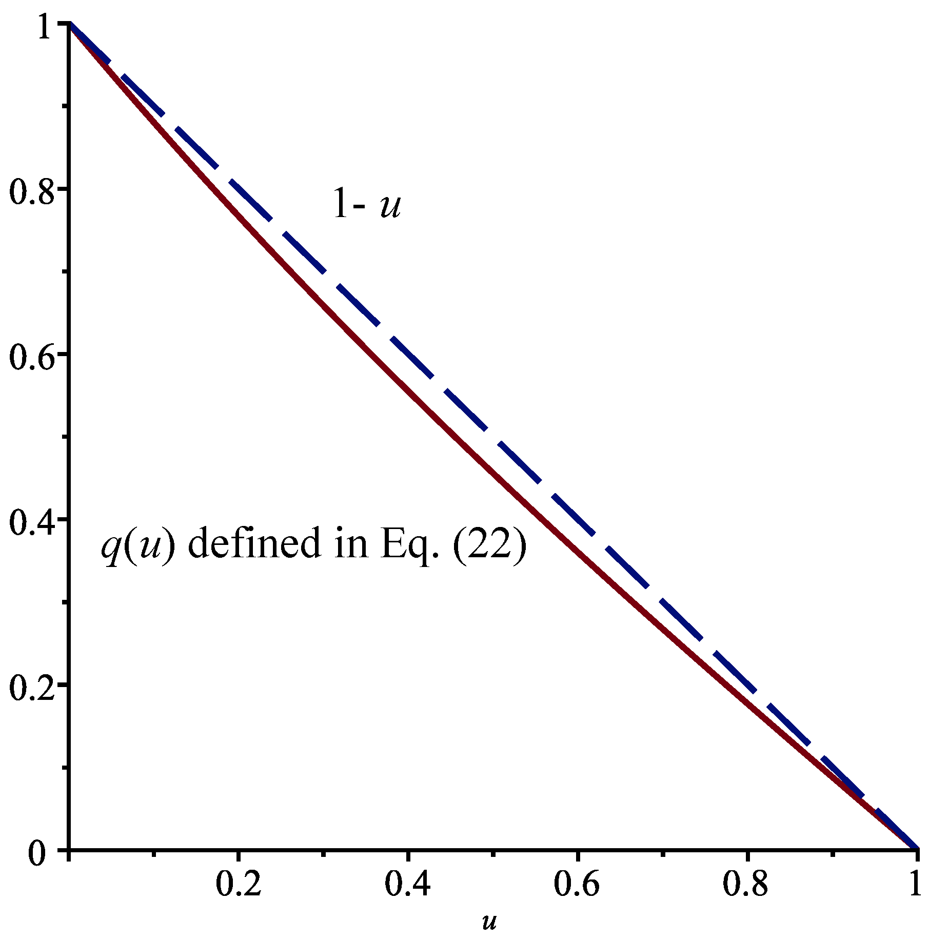
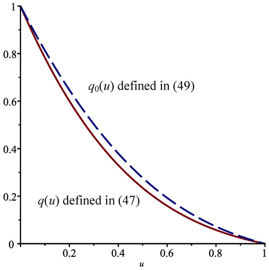
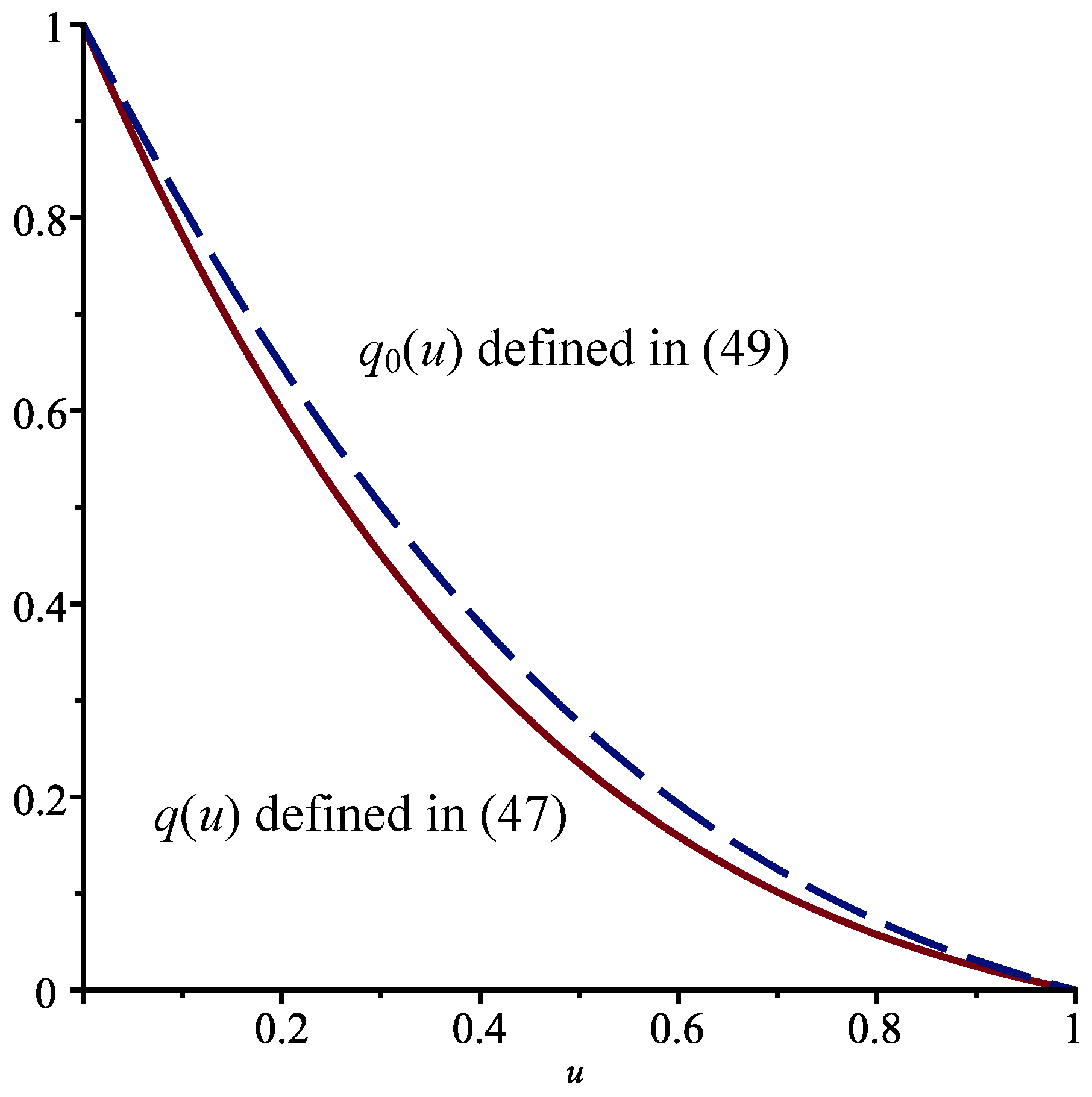
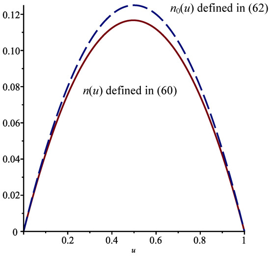
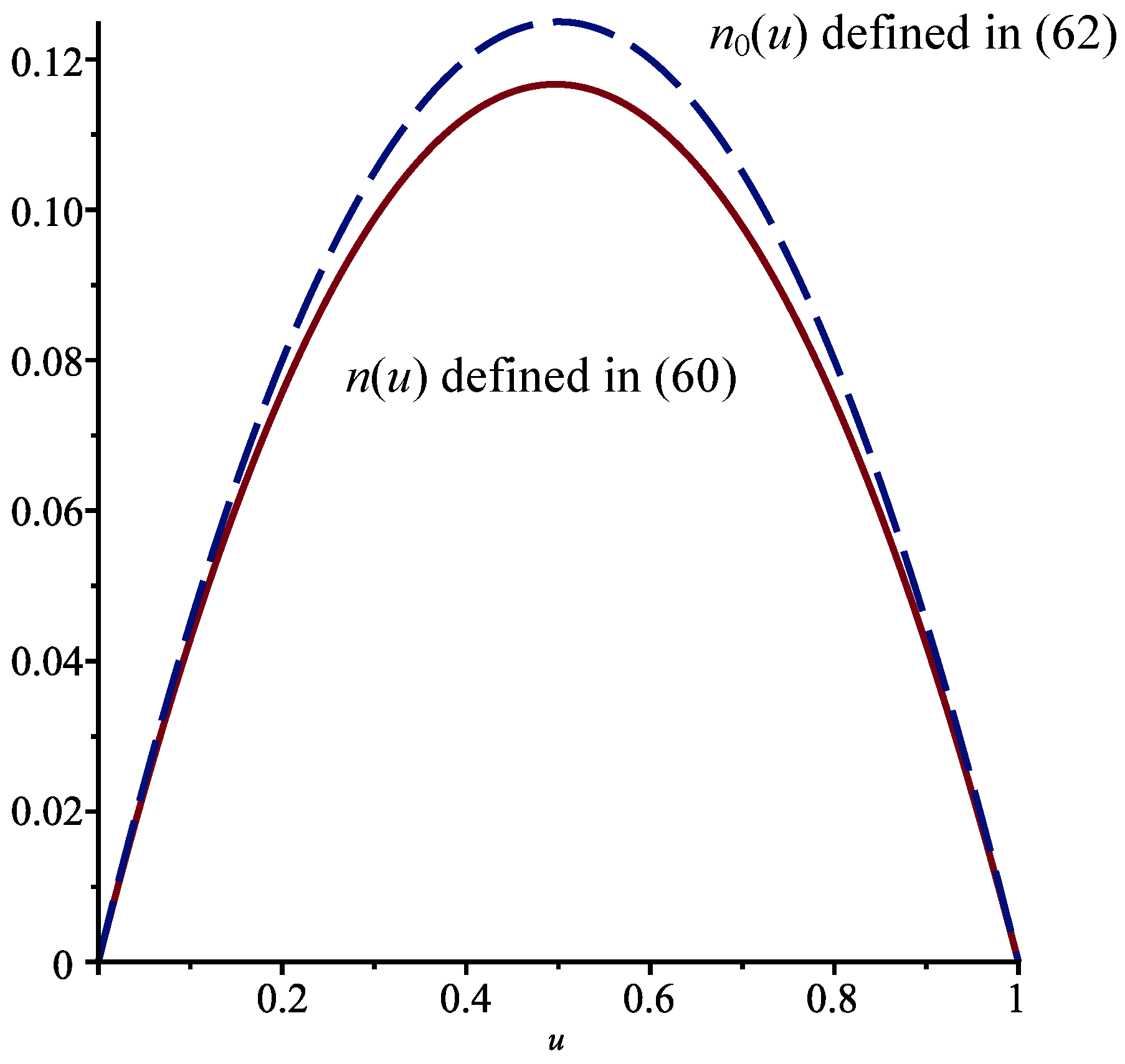
When $\lambda =0$ so that there are no jumps, the function $p_0(x,y)$ that corresponds to $p(x,y)$ can be written as $q_0\left(u\right)$, where $q_0\left(u\right)$ satisfies the elementary ODE

$$q_0^{\prime \prime }\left(u\right)=0.$$

(25)

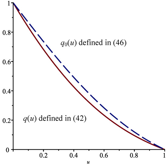
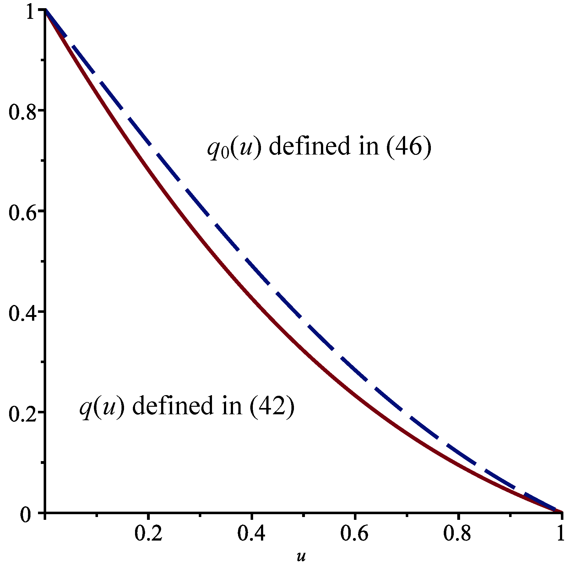
The solution that satisfies the boundary conditions $q_0\left(0\right)=1$ and $q_0\left(1\right)=0$ is $q_0\left(u\right)=1-u$. In Figure 2, the functions $q\left(u\right)$ and $q_0\left(u\right)$ are shown in the interval $[0,1]$. Notice the effect of the jumps on the probability of absorption at $k_1=0$. The effect would be more pronounced if we increased the value of the parameter $\lambda$ and/or decreased $\theta$.

Figure 2. Functions $q\left(u\right)$ defined in (22) with $r\approx 0.4557$ (full line) and $q_0\left(u\right)=1-u$ in the interval $[0,1]$ when $\gamma =\sigma =\lambda =\theta =1$, $k_1=0$ and $k_2=1$.

Case II. Next, we consider the case when

$$\begin{array}{ccc}\hfill X\left(t\right)& =& X\left(0\right)+c{\int }_0^{t}Y\left(s\right)\mathrm{d}s+{\int }_0^t{\left\{X\left(s\right)\right\}}^{1/2}\mathrm{d}{B}_1\left(s\right),\hfill \end{array}$$

(26)

$$\begin{array}{ccc}\hfill Y\left(t\right)& =& Y\left(0\right)-c{\int }_0^{t}Y\left(s\right)\mathrm{d}s+{\int }_0^t{\left\{Y\left(s\right)\right\}}^{1/2}\mathrm{d}{B}_2\left(s\right)+\sum _{i=0}^{N\left(t\right)}{Z}_i,\hfill \end{array}$$

(27)

where $c>0$. This time, $\left\{Y\right(t),t\ge 0\}$ is a jump-diffusion process whose continuous part is a geometric Brownian motion, which is used extensively in financial mathematics.

We need to solve the following PDIE (see (9)):

$$\begin{array}{ccc}\hfill 0& =& cy{p}_x(x,y)-cy{p}_y(x,y)+{\displaystyle \frac{1}{2}}x{p}_{xx}(x,y)+{\displaystyle \frac{1}{2}}y{p}_{yy}(x,y)\hfill \\ & & +\lambda \left\{{\int }_0^{\infty }p(x,y+z)\theta e^{-\theta z}\mathrm{d}z-p(x,y)\right\}.\hfill \end{array}$$

(28)

As in Case I, we set $p(x,y)=q\left(u\right)$, where $u:=x+y$. The boundary conditions are the same as those in Equation (14), and the PDIE becomes the IDE

$$0={\displaystyle \frac{1}{2}}u{q}^{\prime \prime }\left(u\right)+\lambda \left\{{\int }_u^{k_2}q\left(w\right)\theta e^{-\theta (w-u)}\mathrm{d}z-q\left(u\right)\right\}.$$

(29)

Proceeding as above, we find that Equation (29) is transformed into

$$0={\displaystyle \frac{1}{2}}u{q}^{\prime \prime \prime }\left(u\right)+{\displaystyle \frac{1}{2}}(1-\theta u)q^{\prime \prime }\left(u\right)-\lambda q^{\prime }\left(u\right),$$

(30)

which is again a second-order linear ODE for $Q\left(u\right):=q^{\prime }\left(u\right)$ but with non-constant coefficients. When $\theta =\lambda =1$, the general solution of (30) can be written as follows:

$$q\left(u\right)=\left({\mathit{c}}_{\mathit{1}}-{\mathit{c}}_{\mathit{2}}\right)u{\mathit{e}}^u{\mathrm{Ei}}_1\left(u\right)+c_{3}u{\mathit{e}}^u+{\mathit{c}}_{\mathit{2}},$$

(31)

where ${\mathrm{Ei}}_1\left(u\right)$ is an exponential integral. The function ${\mathrm{Ei}}_a\left(z\right)$ is defined by

$${\mathrm{Ei}}_a\left(z\right)={\int }_1^{\infty }{\mathit{e}}^{-zt}{t}^{-a}\mathrm{d}t.$$

(32)

We take $k_1=0$ and $k_2=1$. The solution for $q\left(0\right)=1$, $q\left(1\right)=0$, and $q\left(0.5\right)=r$ is

$$\begin{array}{ccc}\hfill q\left(u\right)& =& 1-{\displaystyle \frac{1}{{\mathrm{Ei}}_1(1/2)-{\mathrm{Ei}}_1\left(1\right)}}\{2u\left[{\mathrm{Ei}}_1\left(1\right)-{\mathrm{Ei}}_1\left(u\right)\right](r-1)e^{(2u-1)/2}\hfill \\ & & -u\left[{\mathrm{Ei}}_1\left(u\right)-{\mathrm{Ei}}_1(1/2)\right]{\mathit{e}}^{u-1}\}.\hfill \end{array}$$

(33)

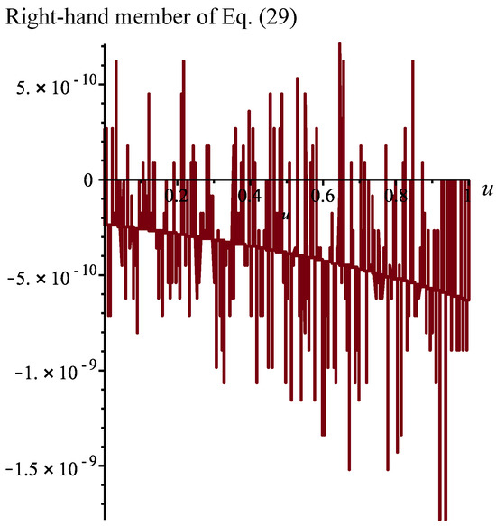
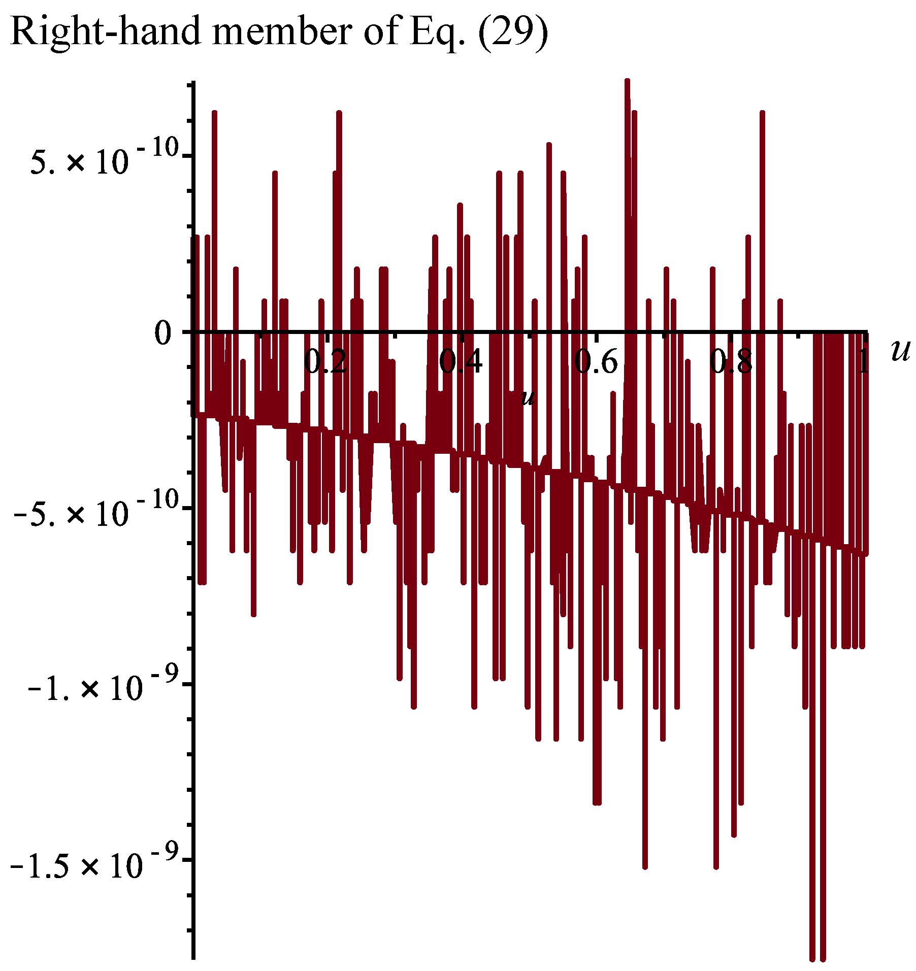
In order for the function defined in Equation (33) to satisfy the PDIE (29), we must take $r\approx 0.2758$. In Figure 3, we present the value of the right-hand member of Equation (29) that we obtain with the function $q\left(u\right)$.

Figure 3. Right-hand member of Equation (29) for $u\in [0,1]$ with the function $q\left(u\right)$ defined in (33) and $r\approx 0.2758$ when $\lambda =\theta =1$, $k_1=0$, and $k_2=1$.

We can state the following proposition.

Proposition 2.

When $\lambda =\theta =1$, $k_1=0$, and $k_2=1$, the function $p(x,y)$ is equal to $q(x+y)$, where $q(·)$ is defined in Equation (33) and $r\approx 0.2758$. We compute

$$p(x,y)\approx 1-(x+y)e^{x+y}\left[1.5{\mathrm{Ei}}_1(x+y)+0.0388\right]$$

(34)

for $0\le x+y\le 1$.

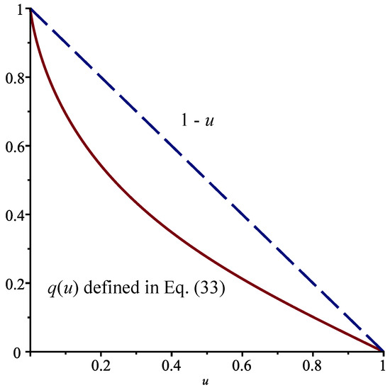
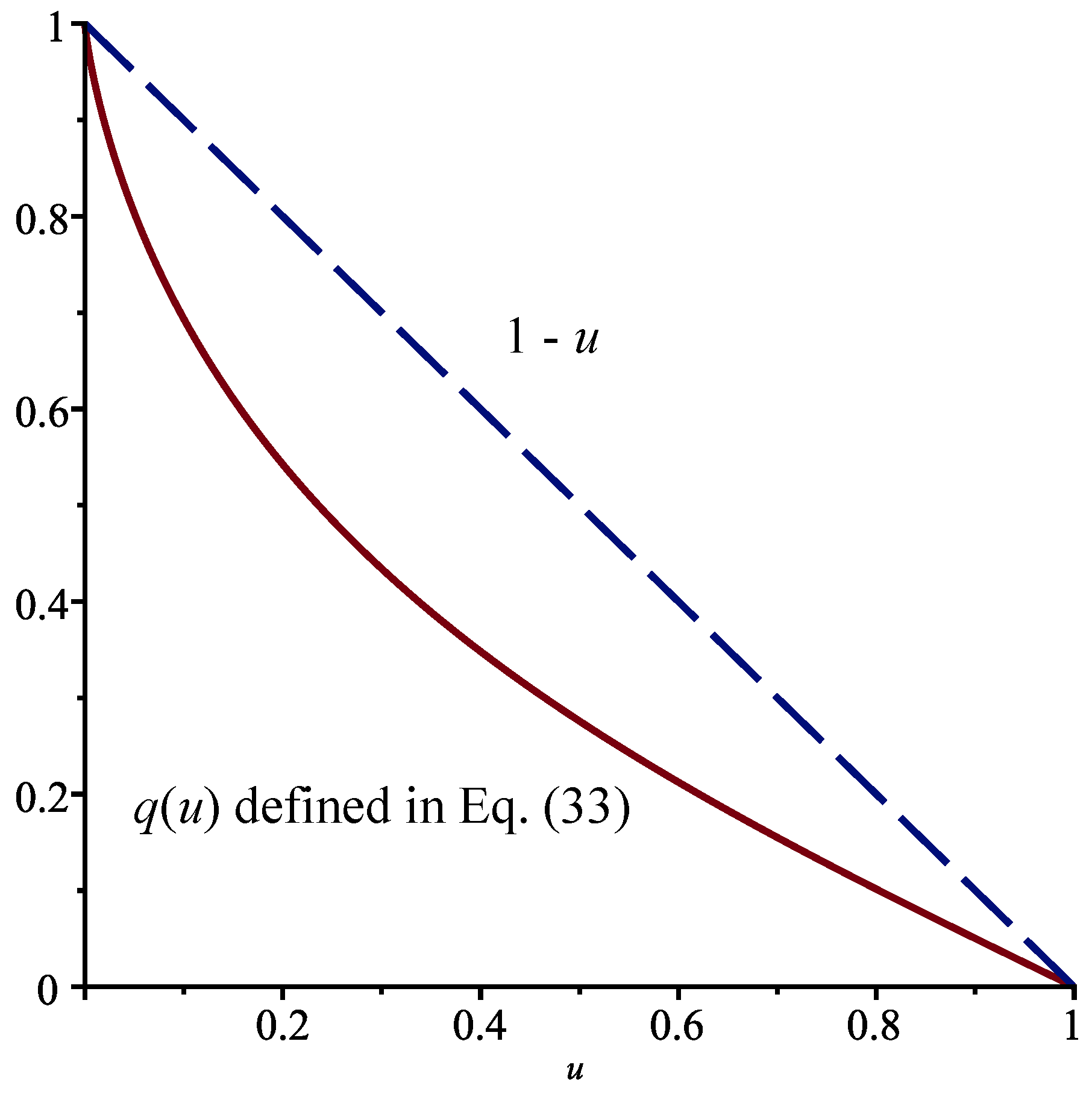
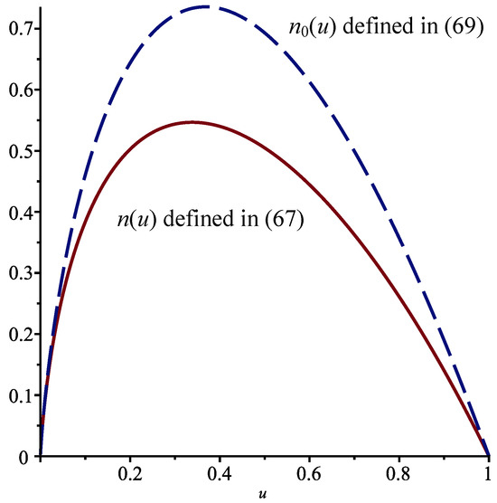
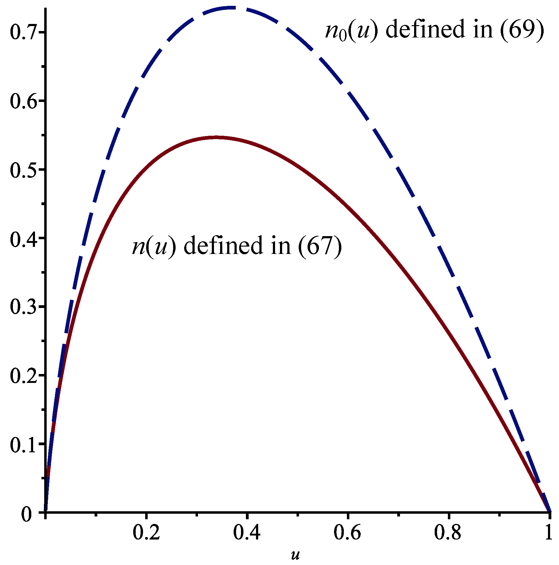
When there are no jumps, the function $q_0\left(u\right)$ is equal to $1-u$, as in Case I, so that $p_0(x,y)=1-(x+y)$. The functions $q\left(u\right)$ and $q_0\left(u\right)$ are displayed in Figure 4 for $u\in [0,1]$. The effect of the jumps is more pronounced than in Case I.

Figure 4. Functions $q\left(u\right)$ defined in (33) with $r\approx 0.2758$ (full line) and $q_0\left(u\right)=1-u$ for $u\in [0,1]$ when $\lambda =\theta =1$, $k_1=0$, and $k_2=1$.

Case III. Finally, we define

$$\begin{array}{ccc}\hfill X\left(t\right)& =& X\left(0\right)+{\int }_0^t[X\left(s\right)+Y\left(s\right)]\mathrm{d}s,\hfill \end{array}$$

(35)

$$\begin{array}{ccc}\hfill Y\left(t\right)& =& Y\left(0\right)+\mu t+{\int }_0^t\sigma \mathrm{d}{B}_2\left(s\right)+\sum _{i=0}^{N\left(t\right)}{Z}_i.\hfill \end{array}$$

(36)

The continuous part of the process $\left\{Y\right(t),t\ge 0\}$ is a Wiener process (or Brownian motion) with drift $\mu \in \mathbb{R}$ and dispersion parameter $\sigma >0$, which is the basic diffusion process. Note that there is a single Brownian motion in the above system so that $\left\{\right(X\left(t\right),Y\left(t\right)),t\ge 0\}$ is a degenerate two-dimensional jump-diffusion process. Moreover, as mentioned in Case I, this type of process is important in reliability theory to model the wear or remaining lifetime of devices.

We deduce from Equation (9) that the function $p(x,y)$ satisfies the PDIE

$$0=(x+y)p_x(x,y)+\mu p_y(x,y)+{\displaystyle \frac{1}{2}}{\sigma }^2{p}_{yy}(x,y)+\lambda \left\{{\int }_0^{\infty }p(x,y+z)\theta e^{-\theta z}\mathrm{d}z-p(x,y)\right\}.$$

(37)

Assuming that $p(x,y)=q\left(u\right)$, with $u:=x+y$, the above equation reduces to

$$0={\displaystyle \frac{1}{2}}{\sigma }^2{q}^{\prime \prime }\left(u\right)+(u+\mu )q^{\prime }\left(u\right)+\lambda \left\{{\int }_u^{k_2}q\left(w\right)\theta e^{-\theta (w-u)}\mathrm{d}z-q\left(u\right)\right\}.$$

(38)

As in the previous cases, the boundary conditions are those in Equation (14).

With $\sigma =\lambda =\theta =1$, we obtain the ODE

$$0={\displaystyle \frac{1}{2}}{q}^{\prime \prime \prime }\left(u\right)+\left(u+\mu +{\displaystyle \frac{1}{2}}\right)q^{\prime \prime }\left(u\right)-(u+\mu )q^{\prime }\left(u\right).$$

(39)

The general solution of this ODE is

$$q\left(u\right)=c_1+c_2{e}^u+c_3\left[e^u\mathrm{erf}\left(u+\mu +{\displaystyle \frac{1}{2}}\right)-e^{-(4\mu +1)/4}\mathrm{erf}\left(u+\mu \right)\right],$$

(40)

where $\mathrm{erf}(·)$ is the error function, which is defined by

$$\mathrm{erf}\left(z\right)={\displaystyle \frac{2}{\sqrt{\pi }}}{\int }_0^z{e}^{-x^2}\mathrm{d}x.$$

(41)

When $k_1=0$, $k_2=1$, and $\mu =0$, we find that the solution such that $q\left(0\right)=1$, $q\left(1\right)=0$, and $q\left(0.5\right)=r$ is

$$\begin{array}{ccc}\hfill q\left(u\right)& =& {\displaystyle \frac{1}{\Omega }}\{\left[(1-r){\mathit{e}}^{{\displaystyle \frac{5}{4}}+u}+r{\mathit{e}}^{u+{\displaystyle \frac{1}{4}}}-{\mathit{e}}^{{\displaystyle \frac{3}{4}}+u}\right]\mathrm{erf}\left(u+{\displaystyle \frac{1}{2}}\right)+\mathrm{erf}\left(3/2\right)(r-1){\mathit{e}}^{{\displaystyle \frac{5}{4}}+u}\hfill \\ & & +{\mathit{e}}^{{\displaystyle \frac{3}{4}}+u}\mathrm{erf}\left(1\right)-r{\mathit{e}}^{u+{\displaystyle \frac{1}{4}}}\mathrm{erf}\left(1/2\right)+\left(r{\mathit{e}}^{{\displaystyle \frac{5}{4}}}+\mathit{e}-{\mathit{e}}^u\right)\mathrm{erf}\left(1/2\right)\hfill \\ & & +\left(-r{\mathit{e}}^{{\displaystyle \frac{5}{4}}}+{\mathit{e}}^{{\displaystyle \frac{7}{4}}}\right)\mathrm{erf}\left(3/2\right)-\mathrm{erf}\left(1\right){\mathit{e}}^{{\displaystyle \frac{7}{4}}}+\left[\mathrm{erf}\left(u\right)-\mathrm{erf}\left(1\right)\right]{\mathit{e}}^{{\displaystyle \frac{1}{2}}}\hfill \\ & & +\left[(1-r){\mathit{e}}^u+r\right]\mathrm{erf}\left(1\right)+\left[(r-1)\mathit{e}-r\right]\mathrm{erf}\left(u\right)\},\hfill \end{array}$$

(42)

where

$$\Omega :=\left({\mathit{e}}^{{\displaystyle \frac{5}{4}}}-{\mathit{e}}^{{\displaystyle \frac{3}{4}}}+\mathit{e}-1\right)\mathrm{erf}(1/2)+\left({\mathit{e}}^{{\displaystyle \frac{7}{4}}}-{\mathit{e}}^{{\displaystyle \frac{5}{4}}}\right)\mathrm{erf}(3/2)+\left({\mathit{e}}^{{\displaystyle \frac{3}{4}}}-{\mathit{e}}^{{\displaystyle \frac{7}{4}}}-{\mathit{e}}^{{\displaystyle \frac{1}{2}}}+1\right)\mathrm{erf}\left(1\right).$$

(43)

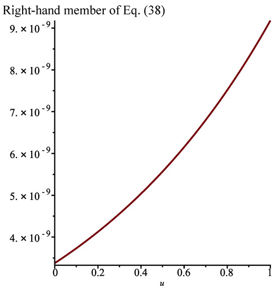
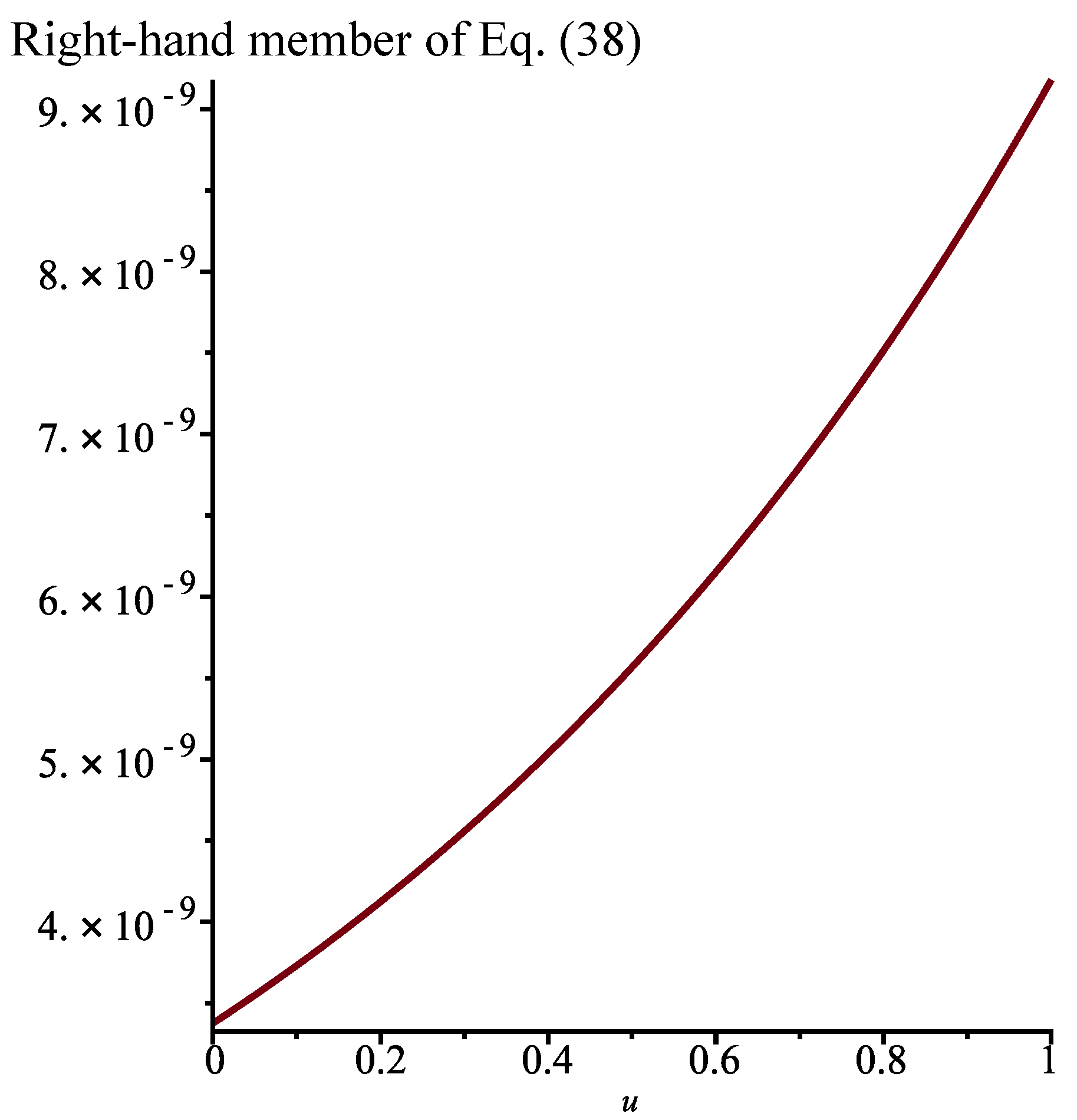
Proceeding as in the previous cases, we find that if $r\approx 0.3223$, then the above function satisfies the PDIE in (38). The right-hand member of Equation (38) obtained with this function is shown in Figure 5.

Figure 5. Right-hand member of Equation (38) for $u\in [0,1]$ with the function $q\left(u\right)$ defined in (42) and $r\approx 0.3223$ when $\sigma =\lambda =\theta =1$, $\mu =0$, $k_1=0$, and $k_2=1$.

Proposition 3.

When $\mu =0$, $\sigma =\lambda =\theta =1$, $k_1=0$, and $k_2=1$, we have $p(x,y)=q(x+y)$, where $q(·)$ is defined in Equation (42) with $r\approx 0.3223$. We can write that

$$\begin{array}{ccc}\hfill p(x,y)& \approx & \left(3.6707{\mathit{e}}^{x+y+1.25}+1.746{\mathrm{e}}^{x+y+0.25}-5.4167{\mathit{e}}^{x+y+0.75}\right)\mathrm{erf}\left(x+y+0.5\right)\hfill \\ & & -3.5462{\mathit{e}}^{x+y+1.25}+4.5646{\mathit{e}}^{x+y+0.75}-0.9088{\mathit{e}}^{x+y+0.25}+2.7404\hfill \\ & & +0.2739{\mathit{e}}^{x+y}-2.7933\mathrm{erf}\left(x+y\right)\hfill \end{array}$$

(44)

for $0\le x+y\le 1$.

Without the jumps, we consider the function $q_0\left(u\right)$, which satisfies the ODE

$${\displaystyle \frac{1}{2}}{q}_0^{\prime \prime }\left(u\right)+u{q}_0^{\prime }\left(u\right)=0.$$

(45)

Making use of the boundary conditions $q_0\left(0\right)=1$ and $q_0\left(1\right)=0$, we find that

$$q_0\left(u\right)=1-{\displaystyle \frac{\mathrm{erf}\left(u\right)}{\mathrm{erf}\left(1\right)}}\mathrm{for}0\le u\le 1.$$

(46)

See Figure 6.

Figure 6. Functions $q\left(u\right)$ defined in (42) with $r\approx 0.3223$ (full line) and $q_0\left(u\right)$ in (46) for $u\in [0,1]$ when $\sigma =\lambda =\theta =1$, $\mu =0$, $k_1=0$, and $k_2=1$.

Finally, with $\mu =1/2$, we obtain that $r\approx 0.2344$ and

$$\begin{array}{ccc}\hfill q\left(u\right)& \approx & \left[2.4884\mathrm{erf}\left(u+1\right)-2.0970\right]{\mathit{e}}^{{\displaystyle \frac{3}{4}}+u}+\left[-10.6146\mathrm{erf}\left(u+1\right)+10.2548\right]{\mathit{e}}^{{\displaystyle \frac{5}{4}}+u}\hfill \\ & & +\left[8.1262\mathrm{erf}\left(u+1\right)-8.0881\right]{\mathit{e}}^{{\displaystyle \frac{7}{4}}+u}+0.2010{\mathit{e}}^u+7.0477\hfill \\ & & -7.0771\mathrm{erf}\left(u+{\displaystyle \frac{1}{2}}\right).\hfill \end{array}$$

(47)

The function $q_0\left(u\right)$ is the unique solution of the ODE

$${\displaystyle \frac{1}{2}}{q}_0^{\prime \prime }\left(u\right)+\left(u+{\displaystyle \frac{1}{2}}\right)q_0^{\prime }\left(u\right)=0$$

(48)

such that $q_0\left(0\right)=1$ and $q_0\left(1\right)=0$. We have

$$q_0\left(u\right)={\displaystyle \frac{\mathrm{erf}\left(u+\frac{1}{2}\right)-\mathrm{erf}\left(\frac{3}{2}\right)}{\mathrm{erf}\left(\frac{1}{2}\right)-\mathrm{erf}\left(\frac{3}{2}\right)}}\mathrm{for}0\le u\le 1.$$

(49)

The functions $q\left(u\right)$ and $q_0\left(u\right)$ are presented in Figure 7.

Figure 7. Functions $q\left(u\right)$ defined in (47) (full line) and $q_0\left(u\right)$ in (49) for $u\in [0,1]$ when $\sigma =\lambda =\theta =1$, $\mu =1/2$, $k_1=0$, and $k_2=1$.

3. Computation of the Mean $\mathit{m}(\mathit{x},\mathit{y})$ and the Moment-Generating Function $\mathit{M}(\mathit{x},\mathit{y})$

In this section, we will first compute the functions $m(x,y)$ and $M(x,y)$ for the process considered in Case I of Section 2. Because the coefficients of the equations that we need to solve are constants, the task is much easier than when these coefficients depend on $u=x+y$, as in Cases II and III. We will also obtain the function $m(x,y)$ in Case II.

First, the PDIE satisfied by the function $M(x,y)$ in Case I is (see Equation (6))

$$\begin{array}{ccc}\hfill \alpha M(x,y)& =& cy{M}_x(x,y)-cy{M}_y(x,y)+{\displaystyle \frac{1}{2}}{\gamma }^2{M}_{xx}(x,y)+{\displaystyle \frac{1}{2}}{\sigma }^2{M}_{yy}(x,y)\hfill \\ & & +\lambda \left\{{\int }_0^{\infty }M(x,y+z)\theta e^{-\theta z}\mathrm{d}z-M(x,y)\right\},\hfill \end{array}$$

(50)

subject to the boundary conditions $M(x,y)=1$ if $x+y=k_1$ or $x+y\ge k_2$.

We look for a solution of the form $M(x,y)=N\left(u\right)$, with $u:=x+y$. This leads to the following equation:

$$\begin{array}{ccc}\hfill \alpha N\left(u\right)& =& {\displaystyle \frac{1}{2}}({\gamma }^2+{\sigma }^2)N^{\prime \prime }\left(u\right)+\lambda \left\{{\int }_0^{\infty }N(u+z)\theta e^{-\theta z}\mathrm{d}z-N\left(u\right)\right\}\hfill \\ & =& {\displaystyle \frac{1}{2}}({\gamma }^2+{\sigma }^2)N^{\prime \prime }\left(u\right)+\lambda \left\{e^{\theta (u-k_2)}+{\int }_u^{k_2}N\left(w\right)\theta e^{\theta (u-w)}\mathrm{d}w-N\left(u\right)\right\}.\hfill \end{array}$$

(51)

Differentiating the above equation with respect to u, we obtain (after some work) that $N\left(u\right)$ satisfies the linear third-order ODE

$${\displaystyle \frac{1}{2}}({\gamma }^2+{\sigma }^2)N^{\prime \prime \prime }\left(u\right)-{\displaystyle \frac{1}{2}}\lambda \theta ({\gamma }^2+{\sigma }^2)N^{\prime \prime }\left(u\right)-(\alpha +\lambda )N^{\prime }\left(u\right)+\alpha \lambda \theta N\left(u\right)=0.$$

(52)

Let us take $\gamma =\sigma =\alpha =\lambda =\theta =1$ so that

$$N^{\prime \prime \prime }\left(u\right)-N^{\prime \prime }\left(u\right)-2N^{\prime }\left(u\right)+N\left(u\right)=0.$$

(53)

We can find the general solution of the above equation. We choose $k_1=0$ and $k_2=1$, and we seek the unique solution for which $N\left(0\right)=N\left(1\right)=1$ and $N\left(0.5\right)=r$. Proceeding as in Section 2, we are able to find the value of the constant r. The resulting expression for the function $N\left(u\right)$ is rather long and will not be reproduced here.

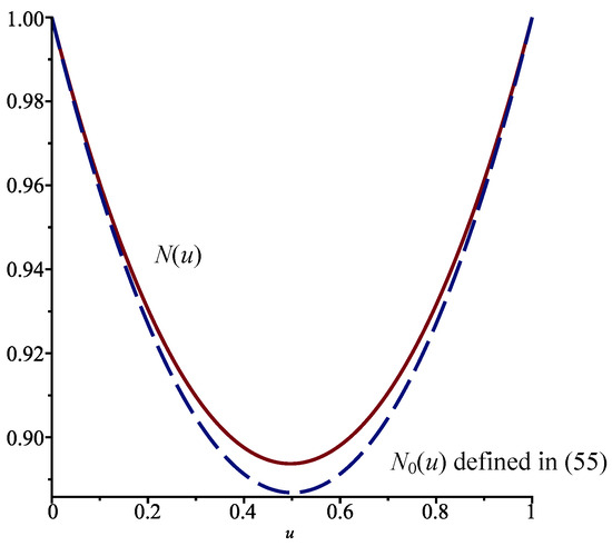
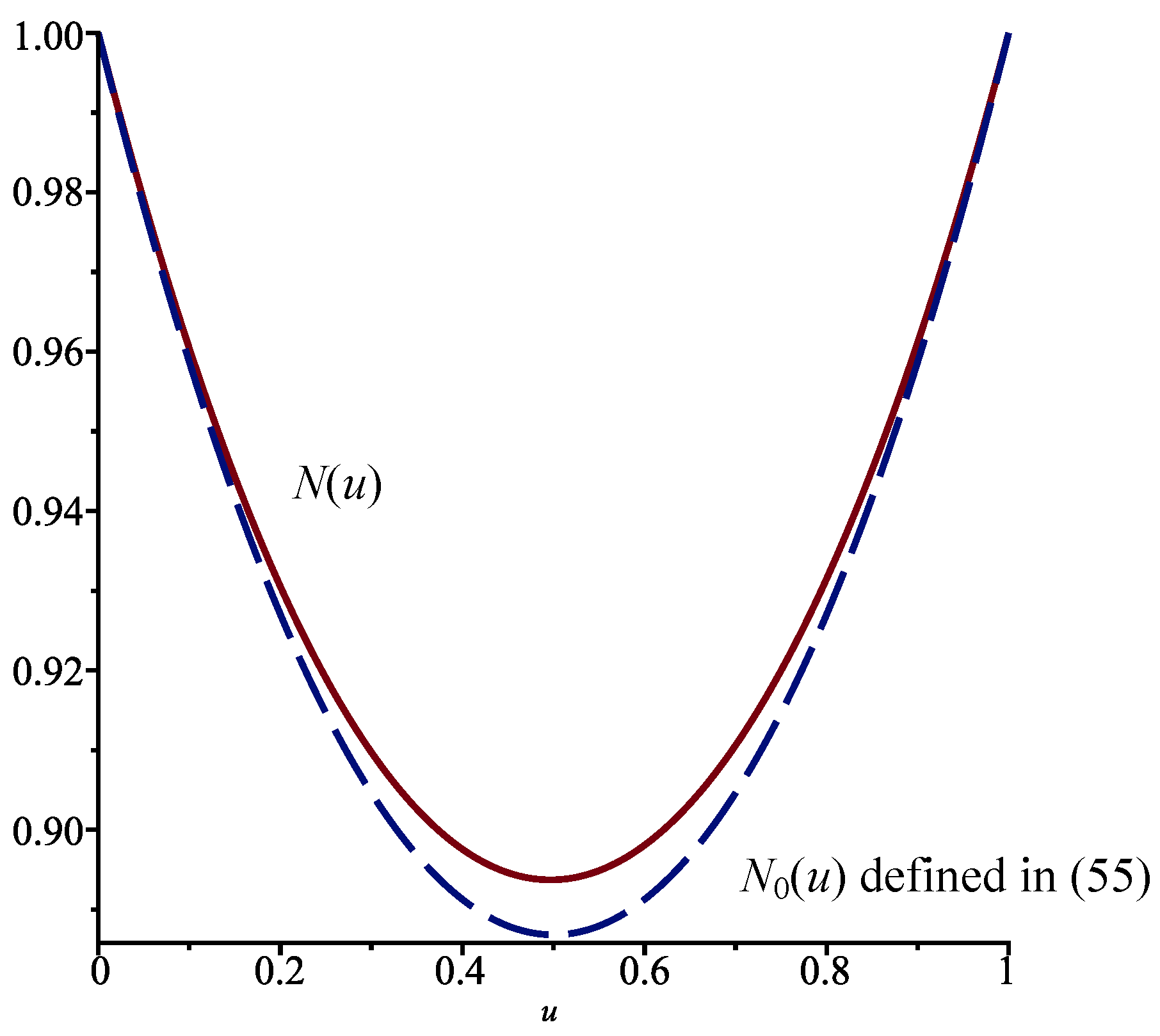
With $\lambda =0$, the function $N_0\left(u\right)$ that corresponds to $N\left(u\right)$ is a solution of the simple ODE

$$N_0^{\prime \prime }\left(u\right)=N_0\left(u\right).$$

(54)

The unique solution such that $N_0\left(0\right)=N_0\left(1\right)=1$ is

$$N_0\left(u\right)={\displaystyle \frac{e^u+e^{1-u}}{e+1}}\mathrm{for}0\le u\le 1.$$

(55)

The functions $N\left(u\right)$ and $N_0\left(u\right)$ are shown in Figure 8.

Figure 8. Functions $N\left(u\right)$ (full line) and $N_0\left(u\right)$ in (55) for $u\in [0,1]$ when $\gamma =\sigma =\alpha =\lambda =\theta =1$, $k_1=0$, and $k_2=1$.

Next, in the case of the function $m(x,y)$, the PDIE is (see Equation (7))

$$\begin{array}{ccc}\hfill -1& =& cy{m}_x(x,y)-cy{m}_y(x,y)+{\displaystyle \frac{1}{2}}{\gamma }^2{m}_{xx}(x,y)+{\displaystyle \frac{1}{2}}{\sigma }^2{m}_{yy}(x,y)\hfill \\ & & +\lambda \left\{{\int }_0^{\infty }m(x,y+z)\theta e^{-\theta z}\mathrm{d}z-m(x,y)\right\},\hfill \end{array}$$

(56)

and we must have $m(x,y)=0$ if $x+y=k_1$ or $x+y\ge k_2$. We define $n\left(u\right)=m(x+y)$, which yields the following ODE:

$${\displaystyle \frac{1}{2}}({\gamma }^2+{\sigma }^2)n^{\prime \prime \prime }\left(u\right)-{\displaystyle \frac{1}{2}}\lambda \theta ({\gamma }^2+{\sigma }^2)n^{\prime \prime }\left(u\right)-\lambda n^{\prime }\left(u\right)=\theta .$$

(57)

Letting $\gamma =\sigma =\lambda =\theta =1$, the above equation simplifies to the ODE

$$n^{\prime \prime \prime }\left(u\right)-n^{\prime \prime }\left(u\right)-n^{\prime }\left(u\right)=1,$$

(58)

whose general solution is

$$n\left(u\right)=-u+c_1+c_{2}exp\left\{{\displaystyle \frac{\left(1+\sqrt{5}\right)u}{2}}\right\}+c_{3}exp\left\{{\displaystyle \frac{\left(1-\sqrt{5}\right)u}{2}}\right\}.$$

(59)

As previously, we can first find the constants $c_i$, $i=1,2,3$, such that $n\left(0\right)=n\left(1\right)=0$ and $n\left(0.5\right)=r$, and then the constant r for which the PDIE is satisfied. The constant is $r\approx 0.1167$ and

$$n\left(u\right)\approx -u+2.5295-0.03689{\mathit{e}}^{1.6180u}-2.4926{\mathit{e}}^{-0.6180u}.$$

(60)

The corresponding function $n_0\left(u\right)$ is the unique solution of

$$n_0^{\prime \prime }\left(u\right)=-1$$

(61)

such that $n_0\left(0\right)=n_0\left(1\right)=0$. We easily find that

$$n_0\left(u\right)={\displaystyle \frac{1}{2}}u(1-u).$$

(62)

See Figure 9.

Figure 9. Functions $n\left(u\right)$ (full line) defined in Equation (60) and $n_0\left(u\right)$ in (62) for $u\in [0,1]$, when $\gamma =\sigma =\lambda =\theta =1$, $k_1=0$ and $k_2=1$.

Finally, in Case II, the PDIE that we need to solve to obtain $m(x,y)=n\left(u\right)$ is

$$-1={\displaystyle \frac{1}{2}}u{n}^{\prime \prime }\left(u\right)+\lambda \left\{{\int }_0^{\infty }n(u+z)\theta e^{-\theta z}\mathrm{d}z-n\left(u\right)\right\}.$$

(63)

This equation is transformed into the ODE

$${\displaystyle \frac{1}{2}}u{n}^{\prime \prime \prime }\left(u\right)+{\displaystyle \frac{1}{2}}(1-\theta u)n^{\prime \prime }\left(u\right)-\lambda n^{\prime }\left(u\right)=\theta .$$

(64)

Choosing $\lambda =\theta =1$, we obtain

$${\displaystyle \frac{1}{2}}u{n}^{\prime \prime \prime }\left(u\right)+{\displaystyle \frac{1}{2}}(1-u)n^{\prime \prime }\left(u\right)-n^{\prime }\left(u\right)=1.$$

(65)

With the help of the software program Maple, we find that the general solution of the above equation is

$$n\left(u\right)=c_1-u+u{e}^u\left[c_2+c_3{\mathrm{Ei}}_1\left(u\right)\right].$$

(66)

Once again, we impose the conditions $n\left(0\right)=n\left(1\right)=0$ and $n\left(0.5\right)=r$. We find that we must take $r\approx 0.5048$. We have

$$\begin{array}{ccc}\hfill n\left(u\right)& \approx & 2.9378u[2.0095{\mathrm{Ei}}_1\left(u\right){\mathit{e}}^{u-1/2}-{\mathrm{Ei}}_1\left(u\right){\mathit{e}}^{u-1}-2.0095{\mathit{e}}^{u-1/2}{\mathrm{Ei}}_1\left(1\right)\hfill \\ & & +{\mathit{e}}^{u-1}{\mathrm{Ei}}_1(1/2)-{\mathrm{Ei}}_1(1/2)+{\mathrm{Ei}}_1\left(1\right)].\hfill \end{array}$$

(67)

In the absence of jumps, we compute the function $n_0\left(u\right)$. It satisfies the ODE

$${\displaystyle \frac{1}{2}}u{n}_0^{\prime \prime }\left(u\right)=-1.$$

(68)

With the conditions $n_0\left(0\right)=n_0\left(1\right)=0$, we find that

$$n_0\left(u\right)=-2uln\left(u\right)\mathrm{for}u\in [0,1].$$

(69)

Figure 10 presents the functions $n\left(u\right)$ and $n_0\left(u\right)$, which are quite different.

Figure 10. Functions $n\left(u\right)$ (full line) defined in Equation (67) and $n_0\left(u\right)$ in (69) for $u\in [0,1]$ when $\lambda =\theta =1$, $k_1=0$, and $k_2=1$.

4. Discussion

In several fields, notably, financial mathematics, many authors are now proposing diffusion processes with jumps as models. Moreover, random variables known as first-hitting times are important in various applications. In two or more dimensions, when there are no jumps, to obtain the quantities of interest, such as the mean of these random variables, we need to solve partial differential equations. These equations become partial differential–integral equations when continuous jumps are added.

In this paper, we have considered problems of this type. Owing to the symmetry in these problems, we were able to reduce the PDIEs to (ordinary) integro-differential equations. For the distribution of the random jumps that we used, we succeeded in transforming the IDEs into ODEs.

We have obtained exact analytical solutions to problems involving important diffusion processes. In cases where it is not possible to find analytical solutions, numerical methods can be used to obtain solutions to problems for fixed values of the various parameters in the models.

To generalize the results obtained in this paper, we could add random jumps to the stochastic process $\left\{X\right(t),t\ge 0\}$ as well. Furthermore, other distributions for the random jumps could be used. For discrete distributions, the equations to be solved would be partial differential–difference equations.

Finally, we could try to solve optimal control problems for these jump-diffusion processes in two or more dimensions. To find the optimal control, in the case of random jumps with a continuous distribution, we generally need to obtain the value function, which would then satisfy a nonlinear PDIE.

References

- Rishel, R. Controlled wear process: Modeling optimal control. IEEE Trans. Autom. Control. 1991, 36, 1100–1102. [Google Scholar] [CrossRef] [Scilit]
- Lefebvre, M. Mean first-passage time to zero for wear processes. Stoch. Models 2010, 26, 46–53. [Google Scholar] [CrossRef] [Scilit]
- Kou, S.G.; Wang, H. First passage times of a jump diffusion process. Adv. Appl. Probab. 2003, 35, 504–531. [Google Scholar] [CrossRef] [Scilit]
- Lefebvre, M. Exact solutions to first-passage problems for jump-diffusion processes. Bull. Pol. Acad. Sci. Math. 2024, 72, 81–95. [Google Scholar] [CrossRef] [Scilit]
- Gihman, I.I.; Skorohod, A.V. Stochastic Differential Equations; Springer: New York, NY, USA; Berlin/Heidelberg, Germany, 1972. [Google Scholar]
- Abundo, M. On first-passage times for one-dimensional jump-diffusion processes. Probab. Math. Statist. 2000, 20, 399–423. [Google Scholar]
- Abundo, M. On the first hitting time of a one-dimensional diffusion and a compound Poisson process. Methodol. Comput. Appl. Probab. 2010, 12, 473–490. [Google Scholar] [CrossRef] [Scilit]
- Abundo, M. On the first-passage area of a one-dimensional jump-diffusion process. Methodol. Comput. Appl. Probab. 2013, 15, 85–103. [Google Scholar] [CrossRef] [Scilit]
- Abundo, M. Some examples of solutions to an inverse problem for the first-passage place of a jump-diffusion process. Control Cybern. 2022, 51, 31–42. [Google Scholar] [CrossRef] [Scilit]
- Merton, R.C. Option pricing when underlying stock returns are discontinuous. J. Financ. Econ. 1976, 3, 125–144. [Google Scholar] [CrossRef] [Scilit]
- Masoliver, J.; Montero, M.; Perelló, J. Jump-diffusion models for valuing the future: Discounting under extreme situations. Mathematics 2021, 9, 1589. [Google Scholar] [CrossRef] [Scilit]
- Cai, N. On first passage times of a hyper-exponential jump diffusion process. Oper. Res. Lett. 2009, 37, 127–134. [Google Scholar] [CrossRef] [Scilit]
- Peng, J.; Liu, Z. First passage time moments of jump-diffusions with Markovian switching. Int. J. Stoch. Anal. 2011, 2011, 1–11. [Google Scholar] [CrossRef] [Scilit]
- Yin, C.; Shen, Y.; Wen, Y. Exit problems for jump processes with applications to dividend problems. J. Comput. Appl. Math. 2013, 245, 30–52. [Google Scholar] [CrossRef] [Scilit]
- Zhou, J.; Wu, L. Occupation times of refracted double exponential jump diffusion processes. Stat. Probab. Lett. 2015, 106, 218–227. [Google Scholar] [CrossRef] [Scilit]
- Gapeev, P.V.; Stoev, Y.I. On the Laplace transforms of the first exit times in one-dimensional non-affine jump–diffusion models. Stat. Probab. Lett. 2017, 121, 152–162. [Google Scholar] [CrossRef] [Scilit]
- Herrmann, S.; Zucca, C. Exact simulation of first exit times for one-dimensional diffusion processes. ESAIM, Math. Model. Numer. Anal. 2020, 54, 811–844. [Google Scholar] [CrossRef] [Scilit]
- Song, S. Some explicit results on first exit times for a jump diffusion process involving semimartingale local time. J. Theor. Probab. 2021, 34, 2346–2367. [Google Scholar] [CrossRef] [Scilit]
- Ai, M.; Zhang, Z.; Yu, W. First passage problems of refracted jump diffusion processes and their applications in valuing equity-linked death benefits. J. Ind. Manag. Optim. 2022, 18, 1689–1707. [Google Scholar] [CrossRef] [Scilit]
Disclaimer/Publisher’s Note: The statements, opinions and data contained in all publications are solely those of the individual author(s) and contributor(s) and not of MDPI and/or the editor(s). MDPI and/or the editor(s) disclaim responsibility for any injury to people or property resulting from any ideas, methods, instructions or products referred to in the content. |
© 2025 by the author. Licensee MDPI, Basel, Switzerland. This article is an open access article distributed under the terms and conditions of the Creative Commons Attribution (CC BY) license (https://creativecommons.org/licenses/by/4.0/).