Abstract
Discriminating between original paintings and replicas is a challenging task. In recent years, the fractal dimension (FD) has been used as a quantitative measure of self-similarity to analyze differences between paintings. However, while the FD parameter has proven effective, previous studies often did not utilize all available image information, typically requiring binarization or grayscale analysis and the manual selection of painting regions. This study introduces a novel, color-FD-based method for differentiating original paintings from replicas. Our approach employs a sliding window approach combined with recent color-FD computation techniques. To assess the effectiveness of our FD methodology, we used two public datasets where originals and replicas were produced by the same artist under identical conditions, ensuring maximum similarity. Statistical comparisons were performed using the nonparametric Wilcoxon rank-sum test. Our method identified significant differences between original and replica paintings for 18 out of 19 pairs across both datasets, outperforming previous studies using the same datasets. As expected, our method discriminates more effectively between paintings by different artists (hit rate of 96.6%) than between originals and replicas by the same artist (hit rate of 91.7%). These findings indicate that combining the FD of color images with a sliding window approach is a promising tool for forgery detection.
1. Introduction
Discriminating between original paintings and replicas presents a significant challenge that requires the integration of diverse evidence, including historical documentation, material analysis, and stylistic comparisons. Despite the meticulous examination of these factors by art experts, definitive conclusions are frequently elusive [1].
Over the past two decades, several computational tools have been proposed to assist experts in differentiating original paintings from replicas. These methodologies primarily rely on the analysis of artist brushstrokes [2,3,4], painting textures and colors [1,5,6,7], and the geometric properties of painting shapes [8,9]. Among the techniques for analyzing paintings, fractal geometry has proven to be a valuable tool for characterizing artists [10,11,12,13,14], pictorial genres [15,16,17,18], and historical periods [19,20,21]. Most of these studies use the fractal dimension (FD), a quantitative metric that describes the complexity with which a shape fills its defined space [22], to analyze the paintings. Shapes that exhibit similar patterns at increasingly smaller scales are called self-similar. Self-similarity, also known as expanding symmetry, is a property analyzed using the FD in various contexts, including the study of natural patterns [23,24].
Using a sliding window to process signals is a widely adopted technique across various fields [25,26,27]. In cultural heritage, this technique has been used to analyze different elements, including buildings, murals, ancient manuscripts, and paintings [28,29,30,31]. The sliding window technique has recently been used to compute the fractal dimension of several types of signals, such as electroencephalograms [32], 4D point clouds [33], time series [34], and medical images [35]. However, to the best of our knowledge, the sliding window approach has not previously been used to analyze the fractal dimension of paintings.
In the present study, we address the following research questions: (1) Is the FD computed from the color information of the images a useful metric for comparing original paintings to replicas? (2) Can the sliding window technique provide a parameterizable solution that avoids the need for the manual selection of painting regions for analysis? (3) Is it possible to obtain comparable or better results than state-of-the-art techniques for forgery detection by integrating color-FD computation into a sliding window approach?
To address these questions, we introduce a novel FD-based methodology for differentiating original paintings from replicas. Recently, several new techniques have been proposed to accurately compute the FD of color images by jointly considering all color channels in the FD estimation process [36,37,38]. Our approach uses one such technique for FD computation [37] by integrating it into a sliding window process of the painting. To the best of our knowledge, this is the first color-FD-based method for distinguishing between original paintings and replicas. Moreover, our methodology does not require the manual selection of painting regions for analysis.
2. Related Work
FD has already been used to differentiate between original paintings and replicas. Taylor et al. [8] analyzed the FD of Jackson Pollock’s paintings, comparing them to similar poured paintings created by art students. In their study, the FD was calculated separately for specific color channels within each painting (black, aluminum, gray, light yellow, and dark yellow) using the box-counting algorithm for binary images [22]. Taylor et al. demonstrated that the FD values of Pollock’s original works exhibited a distinct pattern, meeting specific criteria that were not observed in the FD values of the student-generated paintings.
Abry et al. [5] applied multifractal analysis [39] to differentiate original paintings and replicas created by the same artist under identical conditions (paints, grounds, and brushes). They manually selected corresponding patches from both the original and replica, ensuring consistent spatial location. Subsequently, they calculated the multifractal parameters (hm, c1, and c2) for these selected patches and statistically compared the resulting values between originals and replicas. This multifractal analysis was conducted independently for several image channels (red, green, blue, hue, saturation, lightness, and gray-level intensity). Their findings revealed significant differences in multifractal parameters for five of the seven original–replica pairs.
Recently, Shamir et al. [7] demonstrated that the FD provides the strongest discriminatory power between authentic and non-authentic Jackson Pollock paintings, outperforming a wide range of other image metrics (including texture descriptors, color features, edge statistics, object statistics, distribution of pixel intensity values, multi-scale histograms, and Chebyshev statistics). Shamir et al. estimated the FD using the box-counting algorithm applied to the grayscale images of each painting at multiple resolutions [40].
The FD can also be incorporated as a feature within machine learning algorithms for classifying paintings as originals or replicas, as demonstrated by Albadarneh et al. [6]. In their approach, the painting was divided into a regular grid of patches; then, the image in each patch was binarized using a segmentation algorithm, after which the FD was computed in each binarized patch using the box-counting algorithm [41].
Although the FD parameter has proven its efficacy as a metric for distinguishing between original paintings and replicas, previous studies have not fully utilized all the available information within each painting. Methodologies described in [6,8] require the binarization of the paintings, omitting color information. In [5,7], a broader spectrum of data from each image channel is incorporated into the fractal analysis, but only at the grayscale level. Moreover, several of these methodologies require experts to manually select painting regions for analysis [5], preventing the automated processing of the datasets.
Alternatively, other methodologies [1,3,6] use machine learning classifiers trained using features extracted from each individual patch and tested by classifying individual patches as well. Various types of features are used in these studies, such as those based on the hidden Markov tree multiresolution model in [1], the histogram of oriented gradients technique in [3], and the FD combined with other grayscale and texture features in [6].
3. Material and Methods
3.1. Test Datasets
To assess the efficacy of FD in distinguishing original paintings from replicas, we used two publicly accessible datasets derived from controlled experiments. A notable feature of both datasets is that the originals and replicas were produced by the same artist under identical conditions, ensuring maximum similarity between the paintings. The images in both datasets were obtained from their authors at a very high resolution under the same acquisition conditions for original paintings and replicas, so no further pre-processing was necessary to apply our methodology to them.
The first dataset, which was created by the Machine Learning and Image Processing for Art Investigation Research Group at Princeton University (USA), can be found at https://web.math.princeton.edu/ipai/datasets.html (accessed on 1 May 2025). We refer to this dataset as the Princeton dataset throughout this paper. It has been thoroughly described in previous studies [1,3,5], so we provide only a brief overview here. The Princeton dataset consists of seven original paintings by the artist Charlotte Caspers and their respective replicas, which were painted by the same artist two weeks later (see Figure 1). The original paintings were created using various brushes, canvases, and paints, while the replicas were generated under identical conditions and with the same materials as the corresponding originals. Table 1 shows the relevant data for each original–replica pair within the dataset.
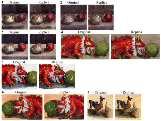
Figure 1.
The Princeton dataset.

Table 1.
Data of paintings in the Princeton dataset.
The second dataset was generated as part of the study by Ji et al. [2] at Case Western Reserve University (Cleveland, OH, USA). This dataset is available for download at https://github.com/hincz-lab/machine-learning-for-art-attribution (accessed on 1 May 2025). Four students from the Cleveland Institute of Art painted three copies of a photograph of a water lily (see Figure 2). All paintings were created using the same oil colors and paintbrushes on paper. The scanned image of each painting measures 3000 × 2400 pixels. We refer to this dataset as the Cleveland dataset throughout this paper.
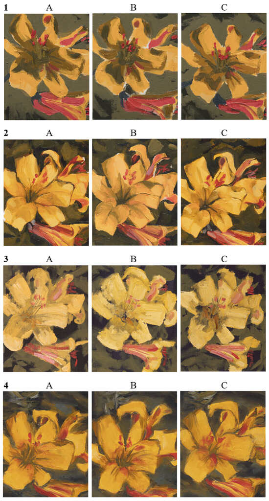
Figure 2.
The Cleveland dataset.
It would be valuable to test our methodology with a dataset including different artistic styles and epochs. However, we were unable to find such a dataset in the public domain. The datasets utilized in this study provide pairs of original–replica paintings that are as similar as possible, as they were created under identical controlled conditions using various canvases, brushes, and paints. Creating such a dataset that also includes significant diversity in artistic styles remains challenging.
3.2. The DBC-RGB Algorithm
As described later, our approach to analyze the paintings involves computing the fractal dimension (FD) of a set of square patches extracted from the paintings. Several methods for estimating the FD of color images have been proposed in recent years [36,37,38,42,43,44,45]. The most common approach has been to extend the differential box-counting (DBC) algorithm for grayscale images to the color domain [36,37,38,44,45]. Among these methods, the ultra-fast DBC-RGB algorithm presented in [37] stands out because its accuracy is comparable to reference algorithms while being much faster due to its parallel nature, which enables GPU implementation. This characteristic is crucial for the present study, as a large number of patches in each painting must be processed. A detailed description of the DBC-RGB algorithm and its GPU implementation can be found in [37]. Below, we briefly describe the fundamentals of the algorithm.
In the DBC-RGB algorithm (see the pseudo-C code in Listing 1), each pixel in the image is represented as a five-dimensional vector (x, y, r, g, b), where (x y) denote the pixel coordinates, while (r, g, b) represent the respective intensity levels of the colors red, green, and blue. The image of M × M pixels is divided into grids of boxes of size s × s, with each grid corresponding to an RGB cube of size h × h × h. Here, h is calculated as , where G is the total number of intensity levels for each color and the grid size s ranges from 2 to . The method then counts the number of boxes of size s × s × h × h × h that cover at least one pixel of the image. To accomplish this, the distribution of pixels along each of the R, G, and B axes is computed independently as follows: (1) For each channel c (R, G, and B) of the image, the boxes containing the maximum and minimum intensity levels within the grid (i, j) are denoted as kc and lc, respectively; and (2) the count for each channel c in the grid (i, j) is then calculated as nrc(i, j) = kc − lc + 1. Once the count nrc(i, j) for each channel is computed, the number nr(i, j) of boxes covering pixels in the grid (i, j) is estimated by multiplying these three counts: nrR(i, j) · nrG(i, j) · nrB(i, j). Finally, the total box count Nr is computed as Nr = for scale r ranging from to , and the fractal dimension of the RGB image is determined by calculating the slope of the linear regression of the points .
A parallel and highly efficient implementation of the DBC-RGB algorithm is achieved in [37] by considering only grid sizes, s, that are powers of two; this approach avoids repeatedly scanning the image to compute each Nr value. The algorithm implementation initializes six buffers (ImaxR, IminR, ImaxG, IminG, ImaxB, and IminB) with the red, green, and blue channels of the image, respectively (see Figure 3a and lines 4–7 in Listing 1). For s = 2, the maximum and minimum intensity levels in each 2 × 2 grid are obtained for each color channel (see Figure 3b and lines 18–25 in Listing 1), and the three counts nrR, nrG, and nrB are calculated. These counts are multiplied to obtain nr; then, Nr is computed as described previously (see lines 26–29 in Listing 1). The maximum and minimum values are then stored in the (0, 0) positions of their respective grids (see yellow cells in Figure 3). For subsequent values of s (s = 4, s = 8, …, and s = ), the algorithm uses the four previously stored values (from the sub-grids) to efficiently obtain the new maximum and minimum values for each grid (see gray cells in Figure 3c,d), avoiding the need to compare all intensities within that grid.
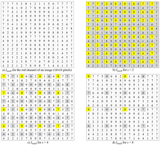
Figure 3.
Maximum value computation for the red channel in the implementation of the DBC-RGB algorithm. For clarity, intensity values range from 0 to 9. Adapted from Figure 2 in [37].
| Listing 1. Pseudo-C implementation of the DBC-RGB algorithm in [37]. |
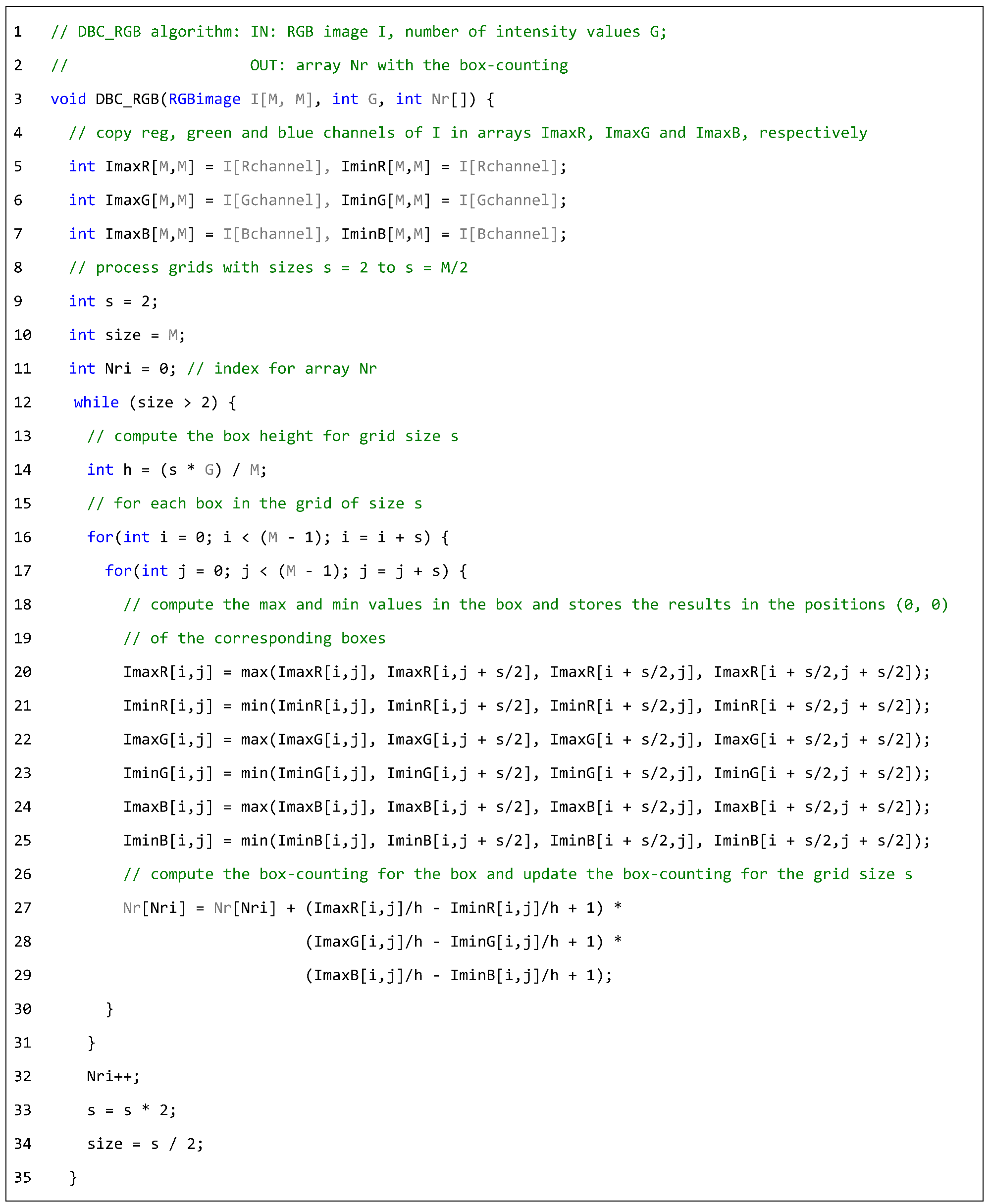 |
To efficiently process the patches within each painting, we used the fast parallel code of the DBC-RGB algorithm, which was implemented in CUDA for GPU execution and made publicly available by its authors in [37].
3.3. The Sliding Window Methodology
The sliding window technique involves dividing the study signal, the image of the painting, into fixed-size segments, called windows. These windows move across the signal with a specified shift, which can be equal to or less than the window length. If the shift is less than the window size, the windows overlap by a certain percentage. Each window is processed individually, and the resulting values are then combined to obtain a representation for the full signal.
Figure 4 graphically illustrates the sliding window computation of the fractal dimension for an original–replica pair of paintings in the Princeton dataset. The sliding window process has two parameters (see Figure 4, step 1): (1) the size of the window, which defines the dimensions of the square patches (e.g., 512 × 512 in the example shown in Figure 4), and (2) the overlap percentage, which establishes the number of pixels that the window shifts by to define the next patch to be processed (e.g., yielding 25% overlap in the example shown in Figure 4). The FD is then computed using the DBC-RGB algorithm for each patch defined by the sliding window (see step 3 in Figure 4). The set of computed FD values from all patches is used to statistically compare the original painting with the replica (see step 4 in Figure 4).
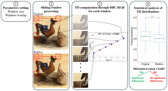
Figure 4.
The sliding window methodology for processing a pair of paintings: (1) selection of values for the following parameters: window size (512 × 512) and window overlap (25%); (2) sliding window computation; (3) example of the FD computation for a window using the DBC-RGB algorithm; and (4) statistical analysis of the distributions of FD values for all windows to identify significant differences between paintings. ****: p-value < 0.0001.
We followed a single criterion when selecting the patch size for processing the two datasets in our study to perform an analysis as similar as possible to those conducted in previous studies using these datasets, ensuring a fair comparison of our results. For the paintings in the Princeton dataset, we selected a window size of 512 × 512 pixels, as recommended in [5]. A patch of 512 × 512 pixels covers approximately 5 × 5 cm2 of the painting surface, which roughly corresponds to the size of the brushstrokes. Moreover, a patch size of 512 × 512 pixels ensures sufficient scale for the linear regression required in the DBC-RGB algorithm’s FD computation. An average correlation coefficient of 0.9997 was obtained for the linear regression calculation performed during FD computation for all 512 × 512-pixel patches across all paintings in the Princeton dataset.
For the paintings in the Cleveland dataset, we used a window size of 256 × 256 pixels. This size, corresponding to a painting patch of approximately 1 × 1 cm2, was selected based on the recommendations in [2], where the authors found that the optimal size for analyzing that dataset ranged between 100 × 100 pixels and 300 × 300 pixels. Since the DBC-RGB algorithm requires patch sizes with dimensions that are powers of two, we considered two possible patch sizes in that range: 128 × 128 and 256 × 256 pixels. Finally, we selected a patch size of 256 × 256 pixels to ensure a wider range of scales for the linear regression calculation in the FD computation, similar to the case with the Princeton dataset. This selection allowed us to obtain an average correlation coefficient of 0.9992 in the linear regression performed during the FD computation for all 256 × 256-pixel patches across all paintings in the Cleveland dataset.
As shown, patch size selection is highly dependent on the characteristics of the painting images being analyzed. General recommendations for selecting the patch size include the following trade-offs: (1) Small patches enable a detailed analysis of the painting but require longer computation times, may overlook key characteristics like brushstroke size, and might not provide a sufficient range of scales for the linear regression calculation in FD computation. (2) Large patches speed up calculations, but they may result in too few FD values for statistical comparisons, as they could be analyzed overly large portions of the painting, thus introducing excessive heterogeneity in terms of painting techniques and brush combinations.
In our experiments, we tested five different window overlap percentages: 0%, 25%, 50%, 75%, and 90%. Rather than seeking optimal values for each dataset, this incremental selection of window overlaps aimed to observe the relationship between this parameter and the emergence of significant differences in painting comparisons. This approach also allows us to identify which painting comparisons might benefit from further analysis with a higher window overlap percentage. Table 2 shows the number of patches generated for paintings in both datasets using each sliding window configuration.
Table 2.
Number of patches generated for each painting using each sliding window configuration. wo: window overlap.
It is not currently possible to automatically determine the optimal window overlap parameter for comparing pairs of paintings in a specific dataset. As we will show in the Section 4, increasing the window overlap percentage leads to identifying more significant differences between paintings within the two datasets, albeit with increased computation times. Therefore, some empirical experimentation is required when analyzing a new dataset, starting with a low value (fastest processing) and then increasing it when no significant differences are found.
Once the window size and overlap percentage are chosen, our methodology operates automatically, eliminating the need for manual patch selection and ensuring a detailed analysis of the entire painting.
The C++ source code for computing the FD of a painting and processing the two datasets using our sliding window methodology is publicly available at https://www.ugr.es/~demiras/swfd (accessed on 1 May 2025).
3.4. Statistical Analysis
To study the differences between the distributions of FD values from patches in original and replica paintings, we performed the nonparametric Wilcoxon rank-sum test (see step 4 in Figure 4). Note that this is the same test used for non-pairwise comparisons in [5]. Since several groups (paintings) were compared simultaneously, the Wilcoxon test was configured with a Bonferroni post hoc correction for multiple comparisons to control the overall probability of making a Type I error. Statistical test results were considered significant when the p-value obtained was below 0.05. All statistical analyses were performed using R version 4.2.1 with the Stats package.
4. Results
4.1. Results on Comparing Paintings
Table 3 shows the statistical comparisons of FD values between pairs of paintings for each tested percentage of window overlap in the sliding window configuration. These results show that as the percentage of window overlap increases, more statistically significant differences (p-value < 0.05) between original and replica paintings are observed across both datasets. This finding indicates that a higher window overlap percentage provides a more detailed analysis of the painting. Our method identified significant differences between original and replica paintings for all pairs in the Princeton dataset. Nevertheless, it did not detect differences between the FD distributions of paintings A and C for artist 2 in the Cleveland dataset. As shown later, the FD distributions for these two paintings are indeed almost identical.
Table 3.
p-Values for the Wilcoxon test comparing the FD values between the original paintings and replicas. wo: window overlap. Statistically significant differences are indicated with a bold p-value.
Figure 5 shows boxplots comparing the FD values between the pairs of original and replica paintings in the Princeton dataset using the sliding window configuration with a 90% window overlap. Table 4 shows the detailed results from our algorithm at 90% window overlap, along with a comparison with the results obtained in [5] for the same dataset using multifractal analysis. The multifractal parameters (hm, c1, and c2) showed significant differences in only three of the seven comparisons between pairs of original and replica paintings [5], whereas our method found significant differences in all seven comparisons. Notably, both methodologies used the same statistical test (Wilcoxon rank-sum test) to compare the distributions of measures obtained from the paintings.
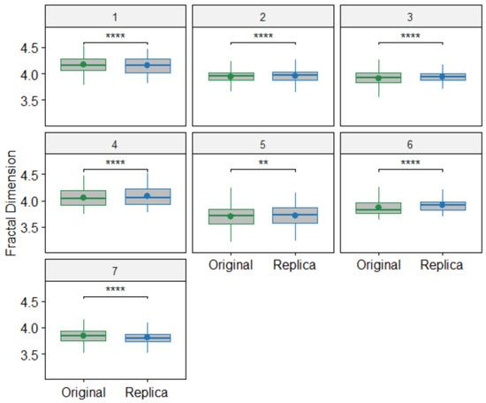
Figure 5.
Boxplots showing significant differences between the original and replica paintings in the Princeton dataset. **: p-value < 0.01 and ****: p-value < 0.0001.
Table 4.
Comparison between our results (Sliding window FD) and multifractal results from Abry et al. for the Princeton dataset [5]. The sliding window FD algorithm was executed with a 90% window overlap. FD: average FD, Std: standard deviation. All p-values correspond to Wilcoxon rank-sum tests. Statistically significant differences are indicated with a bold p-value.
Regarding the average FD values shown in Table 4 for the Princeton dataset, most replica paintings (five out of seven) exhibit higher FD values than their corresponding originals. As expected, the average FD values and the standard deviations are very close for all pairs of paintings, indicating a high degree of similarity between the originals and their replicas.
For the Cleveland dataset, Figure 6 shows boxplots comparing the FD values between paintings by the same artist using the sliding window configuration with a 90% window overlap. Table 5 provides the corresponding results, including average FD values and standard deviations for each painting.
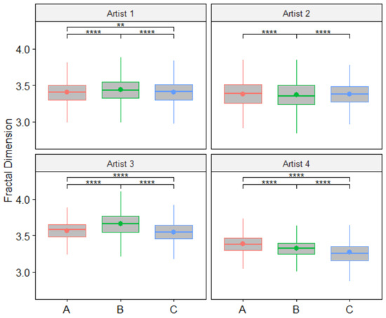
Figure 6.
Boxplots showing significant differences between paintings in the Cleveland dataset. **: p-value < 0.01 and ****: p-value < 0.0001.
Table 5.
Detailed results of the window sliding FD algorithm with a 90% window overlap for the Cleveland dataset. FD: average FD, Std: standard deviation, p-value: p-value for the Wilcoxon rank-sum test. 1: p-value for the A-B comparison, 2: p-value for the B-C comparison, 3: p-value for the C-A comparison. Statistically significant differences are indicated with a bold p-value.
For the Cleveland dataset, a direct comparison between our results and those obtained in [2] is not possible because their goal was to classify the paintings according to the artist, rather than to differentiate between paintings by the same artist.
As shown in Table 5, our results for this dataset show more variability in the average FD values among paintings by the same artist. This explains why a lower percentage of window overlap in the algorithm (implying a less detailed analysis of the paintings) was sufficient to obtain significant differences (see Table 3).
Given that the Cleveland dataset includes works from four artists, it was also possible to compare the FD between pairs of paintings where one painting was by one artist and the other was by a different artist. In this case, 58 pairs of paintings were compared (e.g., 1-A to 2-A, 1-A to 2-B, 1-A to 2-C, 1-B to 2-A, etc.) using the same five sliding window configurations. Table 6 presents the results showing the number of pairs of paintings and the percentage of the total pairs that exhibit significant differences in the FD. These results are also compared in Table 6 with those obtained from comparing pairs of paintings by the same artist (results extracted from Table 3).
Table 6.
Significant differences in FD between pairs of paintings in the Cleveland dataset when comparing pairs by the same artist and pairs painted by different artists for each sliding window configuration. #Pairs: number of pairs compared, #SD: number of pairs showing significant differences in FD, % SD: percentage of pairs with significant differences, wo: window overlap.
More significant differences in FD were found when comparing pairs of paintings by different artists. Additionally, high percentages of significant differences were observed with smaller window overlap percentages when the compared pairs were by different artists. Therefore, as expected, the method discriminated more effectively between paintings by different artists than between paintings by the same artist, requiring a lower window overlap to achieve significant differentiation.
4.2. Results on Comparing Artists
We also compared the FD distributions between the four artists in the Cleveland dataset. In this case, the values compared between artists correspond to the pooled set of FD values from all three of their respective paintings. This comparison is not about differentiating originals from replicas, but rather about distinguishing between artists based on their styles or “artist hand”. Table 7 shows the statistical comparisons of FD values between the four artists in the Cleveland dataset for each tested window overlap percentage in the sliding window configuration used to process each painting. These results show that all comparisons found significant differences between the artists. This indicates that our proposed FD methodology can distinguish not only between original paintings and replicas by the same or different artists but also between sets of similar paintings created under identical conditions by different artists.
Table 7.
p-values for the Wilcoxon test comparing the FD values between the artists in the Cleveland dataset. All differences between artists are statistically significant. wo: window overlap.
Figure 7 shows boxplots comparing the FD values between the artists in the Cleveland dataset using the sliding window configuration with a 0% window overlap.
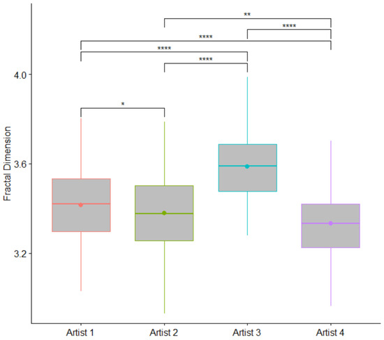
Figure 7.
Boxplots showing significant differences in FD between the artists in the Cleveland dataset. Paintings for each artist were processed with a window overlap percentage of 0%. *: p-value < 0.05, **: p-value < 0.01 and ****: p-value < 0.0001.
4.3. Performance Analysis
Finally, we conducted a performance analysis of our algorithm. For time measurements, we used the now method of the high_resolution_clock class in the chrono C++ library, providing millisecond precision. We sequentially processed the two datasets (one painting after the other) on a computing server with the following configuration: Debian Linux 5.10 operating system, Intel Xeon Silver 4210 @ 2.20 GHz (10 cores and 20 threads), 96 GB of RAM, three GPUs, an NVIDIA GeForce RTX 3090 with 10,496 CUDA cores and 24 GB of global memory, and two NVIDIA GeForce RTX 2080 Ti GPUs, each with 4352 CUDA cores and 11 GB of global memory. Additionally, we processed the paintings in both datasets in parallel using OpenMP technology [46] within our C++ code. Table 8 shows the times required to process each dataset for each window overlap configuration in two scenarios: sequential processing of paintings and parallel processing of paintings.
Table 8.
Execution times (T, in seconds) and megapixels per second (MP/s) for dataset processing with window overlap (wo) configurations.
Although the sequential processing times for high window overlaps may appear lengthy (approximately averaging 6.5 s per image with a 90% window overlap), this is primarily due to the large number of patches processed (between 9500 and 13,500 patches per image at a 90% window overlap). Nonetheless, processing such a large number of patches per image provides a very detailed analysis. Furthermore, without the recently released ultra-fast GPU algorithm for computing the FD of each patch, as provided in [37], the processing times would have been up to eight times slower, in comparison to other parallel GPU algorithms for FD computation [37]. Compared to sequential CPU implementations of color-FD algorithms with similar accuracy [36], the processing times required for the two datasets would have been up to nine hundred times slower [37], resulting in approximately two days of computation.
Parallel processing of the paintings significantly improved performance. The multi-threaded OpenMP execution of the experiment on a server equipped with three GPUs greatly reduced the time required to process all the paintings in both datasets. As shown in Table 8, with a window overlap of 90%, the total processing time for all paintings decreased from 168.69 s (sequential) to 54.21 s (parallel). With a 0% window overlap, the total processing time decreased from 2.90 s (sequential) to 1.12 s (parallel). This speedup implies that our software would be able to process up to 1725 images with a 90% window overlap or 83,720 images with a 0% window overlap, where each image has an average high-resolution size of 4092 × 4369 pixels, all within just one hour. This demonstrates the efficiency of our methodology in processing extensive image datasets.
The difference in megapixels processed per second (MP/s in Table 8) between the two datasets is due to the fact that the Princeton dataset used a patch size of 512 × 512, while the Cleveland dataset used a patch size of 256 × 256. This means that each patch in the Princeton dataset processed four times as many pixels as in the Cleveland dataset. Therefore, the selected patch size affects the execution time; however, in our study, the patch sizes were chosen based on the characteristics of the images, following the same criteria as in [2,5].
5. Discussion and Conclusions
In this study, we introduced a novel, color-FD-based method for differentiating original paintings from replicas. By using a sliding window approach and recent color-FD computation techniques [37], our method effectively analyzed two public datasets, identifying significant differences between original and replica paintings. These findings suggest that combining the FD of color images with a sliding window approach is a promising tool for forgery detection.
Previous multifractal analysis of the Princeton dataset [5] revealed significant differences in only three of seven original–replica painting comparisons, whereas our method, employing the same statistical test, detected significant differences in all seven. This enhanced performance required a more intensive image analysis, using a 90% window overlap, in contrast to the expert-driven manual patch selection employed by the multifractal approach in [5].
The analysis of the Princeton dataset revealed that most replica paintings had higher average FD values compared to their original counterparts (see Table 4 and Figure 5). This finding aligns with the increased multifractal parameter values reported in [5] for cases where significant differences between originals and replicas were detected. In the case of original paintings, the artist’s hand movements, brush strokes, and color application may be more spontaneous and natural, leading to a lower FD value. Replicas, on the other hand, might be created with a more deliberate and controlled approach, as the artist attempted to replicate the original work. This more methodical process could result in a higher FD value due to the presence of more intricate and detailed patterns. In contrast, in the Cleveland dataset, we did not observe a similar pattern in the average FD values. This discrepancy may be attributed to the fact that all three paintings by each artist in the Cleveland dataset are copies of a photograph rather than replicas of an original painting.
While FD distributions are quite similar for paintings in the Princeton dataset, greater variability in FD distribution is observed in paintings by the same artist in the Cleveland dataset. One possible reason is that the artist in the first dataset was instructed to make the replica paintings as faithful to the originals as possible. However, for the second dataset, the artists were simply instructed to make copies of the water lily photograph, ensuring that the copies maintained the same style.
The Cleveland dataset allowed us to test our methodology by comparing pairs of paintings by the same artist as well as similar paintings from different artists created under identical controlled conditions. This scenario closely resembles the typical forgery detection problem addressed in several recent studies [2,7]. Our results indicate that the methodology was able to identify significant differences in nearly all comparisons: 96.6% when comparing pairs of paintings from different artists (see Table 6) and 100% for inter-artist comparisons (see Table 7). Although accuracy metrics vary across studies, our results are comparable to or better than those in recent forgery detection research: 95% accuracy in [2] and a 96% hit rate in [7].
Previous studies that used the Princeton dataset [1,3,6] did not compare original paintings and replicas directly; instead, they used machine learning classifiers that were trained with the features extracted from each individual patch and tested by classifying individual patches as well. This analysis of original–replica paintings is different from the approach followed in [5] and in our study, so their results cannot be directly compared to ours and those obtained in [5]. Nevertheless, these studies based on machine learning classifiers provided metrics of accuracy for the classification of patches, and if we consider that an accuracy value above 75% for correctly classifying these patches is equivalent to a correct distinction between the original painting and its replica, then we can make a kind of comparison between the results of those previous studies based on machine learning and our results. In [1], a hidden Markov tree multiresolution model was used to extract the features for each patch, and their best classification technique correctly distinguished originals from replicas in three out of seven pairs of paintings in the Princeton dataset. In [3], the features computed for each patch were based on the histogram of oriented gradients technique, and they correctly classified seven out of seven pairs of paintings in the Princeton dataset, obtaining an equivalent result to ours. The last study analyzing the Princeton dataset was conducted in [6]. They extracted a total of 153 features for each patch, and their best result achieved correct classification in three out of seven pairs of paintings.
Two other studies in forgery detection analyzed abstract paintings by the artist Jackson Pollock and fake paintings attempting to imitate his unique style [7,8]. Although these studies did not try to differentiate between originals and replicas of the same painting, their results demonstrate that FD features provide strong discriminatory power between authentic and fake Jackson Pollock paintings. In these two studies, the FD was computed on the grayscale representation [7] or via black-and-white binarization [8] of the image of the painting. Our results using the FD at the color level of images suggest that their results could be further improved by applying FD computation algorithms such as DBC-RGB.
Since the present study has proven the effectiveness of our FD-based methodology for differentiating between original paintings and replicas, further research could also be directed towards incorporating the FD value computed at each individual patch through the DBC-RGB algorithm as a feature in machine learning models used in previous studies [1,2,3,6]. Among them, only the model described in [6] incorporated the FD as one of the features describing each patch. However, they used an FD computation approach based on the pre-binarization of the patches. We think that processing the full color information using algorithms such as DBC-RGB could further enhance the results of these machine learning classifiers.
Our methodology requires establishing two key parameters: patch size and window overlap percentage. To ensure fair comparisons in the present work, we selected the same patch sizes recommended by the studies that analyzed the same datasets [2,5]. In general, small patches allow for a detailed analysis of the painting but at the cost of longer computation times and potentially overlooking key painting characteristics such as the size of the brushstrokes. Conversely, large patch sizes accelerate the calculations, but the number of FD values for statistical comparisons of the paintings could be insufficient, and the portion of the painting analyzed in each patch could be too large, including too much heterogeneity (painting techniques and combinations of brushes). According to our experiments, increasing the window overlap percentage leads to the detection of a greater number of significant differences between paintings within the datasets. While a higher window overlap parameter value allows for more detailed analysis, it also demands longer computation times. Nevertheless, establishing a high window overlap does not ensure finding significant differences when comparing every pair of paintings, as seen in the case of paintings A and C by artist 2 in the Cleveland dataset. This pair of paintings was further examined using extremely high window overlaps of 95% and 99%, yet no significant differences were found. Unfortunately, we cannot provide general rules or criteria for automatically determining the optimal patch size and window overlap parameters. Therefore, some empirical experimentation is required depending on the characteristics of the dataset of paintings being analyzed.
In order to use our approach on other datasets, the following considerations must be taken into account: (1) High-resolution images are needed to capture as much as possible the subtle details of the paintings that can differentiate between originals and replicas. (2) Since the FD computation method in our methodology is based on the color intensities, the acquisition of images for each original–replica pair must be performed under identical conditions, and (3) the patch size in sliding window processing must be large enough to obtain a number of scales that ensure an accurate linear regression computation in the FD estimation through the DBC-RGB algorithm (at least 128 × 128 pixels as suggested in [37]). Images of the paintings at a low resolution could imply that the patch size does not meet this requirement.
The primary limitation of our sliding window FD algorithm is its high computational demand, particularly when processing high-resolution images with a large window overlap. Unfortunately, prior related studies have not reported the computation times of their respective algorithms, making it impossible to make a direct performance comparison. Nonetheless, given that our methodology is based on a fast algorithm executed in parallel on a GPU [37], we believe that our computation times would not be significantly worse than those obtained in similar studies, particularly those that also process grids of patches within the painting [1,2,3,6]. As we demonstrated with our OpenMP implementation, the overall dataset processing can be significantly optimized through the parallel processing of multiple paintings. In this scenario, the number of paintings processed concurrently depends on the available GPUs, CPU cores, RAM, and GPU global memory of the computing system.
Author Contributions
Methodology, J.R.d.M. and D.M.; software, J.R.d.M.; validation, J.R.d.M. and D.M.; investigation, J.R.d.M.; resources, J.R.d.M. and D.M.; writing—original draft preparation, J.R.d.M.; writing—review and editing, J.R.d.M. and D.M; and project administration, J.R.d.M. and D.M. All authors have read and agreed to the published version of the manuscript.
Funding
This research was partially funded by the Spanish Ministry of Economy and Competitiveness (grant number PID2020.118638RB.I00).
Data Availability Statement
The data and source code presented in this study are publicly available at https://www.ugr.es/~demiras/swfd (accessed on 1 May 2025).
Conflicts of Interest
The authors declare that they have no conflicts of interest.
References
- Polatkan, G.; Jafarpour, S.; Brasoveanu, A.; Hughes, S.; Daubechies, I. Detection of Forgery in Paintings Using Supervised Learning. In Proceedings of the 2009 16th IEEE International Conference on Image Processing (ICIP), Cairo, Egypt, 7–10 November 2009; pp. 2921–2924. [Google Scholar]
- Ji, F.; McMaster, M.S.; Schwab, S.; Singh, G.; Smith, L.N.; Adhikari, S.; O’Dwyer, M.; Sayed, F.; Ingrisano, A.; Yoder, D.; et al. Discerning the Painter’s Hand: Machine Learning on Surface Topography. Herit. Sci. 2021, 9, 152. [Google Scholar] [CrossRef]
- Buchana, P.; Cazan, I.; Diaz-Granados, M.; Juefei-Xu, F.; Savvides, M. Simultaneous Forgery Identification and Localization in Paintings Using Advanced Correlation Filters. In Proceedings of the International Conference on Image Processing, ICIP; IEEE Computer Society, Phoenix, AZ, USA, 3 August 2016; Volume 2016, pp. 146–150. [Google Scholar]
- Bigerelle, M.; Guibert, R.; Mironova, A.; Robache, F.; Deltombe, R.; Nys, L.; Brown, C.A. Fractal and Statistical Characterization of Brushstroke on Paintings. Surf. Topogr. Metrol. Prop. 2023, 11, 15019. [Google Scholar] [CrossRef]
- Abry, P.; Wendt, H.; Jaffard, S. When Van Gogh Meets Mandelbrot: Multifractal Classification of Painting’s Texture. Signal Process. 2013, 93, 554–572. [Google Scholar] [CrossRef]
- Albadarneh, I.A.; Ahmad, A. Machine Learning Based Oil Painting Authentication and Features Extraction. Int. J. Comput. Sci. Netw. Secur. 2017, 17, 8–17. [Google Scholar]
- Shamir, L. Computer Vision Profiling and Identification of Authentic Jackson Pollock Drip Paintings. Arts Commun. 2024, 2, 1628. [Google Scholar] [CrossRef]
- Taylor, R.P.; Guzman, R.; Martin, T.P.; Hall, G.D.R.; Micolich, A.P.; Jonas, D.; Scannell, B.C.; Fairbanks, M.S.; Marlow, C.A. Authenticating Pollock Paintings Using Fractal Geometry. Pattern Recognit. Lett. 2007, 28, 695–702. [Google Scholar] [CrossRef]
- de la Calleja, E.M.; Zenit, R. Topological Invariants Can Be Used to Quantify Complexity in Abstract Paintings. Knowl.-Based Syst. 2017, 126, 48–55. [Google Scholar] [CrossRef]
- Balankin, A.; Márquez, J. Fractal Analysis of Paintings. Científica 2003, 7, 129–137. [Google Scholar]
- Gerl, P.; Schönlieb, C.; Wang, K. The Use of Fractal Dimension in Arts Analysis. Harmon. Fractal Image Anal. 2004, 1, 70–73. [Google Scholar]
- Bountis, T.; Fokas, A.S.; Psarakis, E.Z. Fractal Analysis of Tree Paintings by Piet Mondrian (1872–1944). Int. J. Arts Technol. 2017, 10, 27–42. [Google Scholar] [CrossRef]
- de la Calleja, E.; Zenit, R. Fractal Dimension and Topological Invariants as Methods to Quantify Complexity in Yayoi Kusama’s Paintings. arXiv 2020, arXiv:2012.06108. [Google Scholar]
- Turkheimer, F.E.; Liu, J.; Fagerholm, E.D.; Dazzan, P.; Loggia, M.L.; Bettelheim, E. The Art of Pain: A Quantitative Color Analysis of the Self-Portraits of Frida Kahlo. Front. Hum. Neurosci. 2022, 16, 1000656. [Google Scholar] [CrossRef] [PubMed]
- Redies, C.; Brachmann, A. Statistical Image Properties in Large Subsets of Traditional Art, Bad Art, and Abstract Art. Front. Neurosci. 2017, 11, 593. [Google Scholar] [CrossRef]
- Mather, G. Aesthetic Image Statistics Vary with Artistic Genre. Vision 2020, 4, 10. [Google Scholar] [CrossRef] [PubMed]
- Peptenatu, D.; Andronache, I.; Ahammer, H.; Taylor, R.; Liritzis, I.; Radulovic, M.; Ciobanu, B.; Burcea, M.; Perc, M.; Pham, T.D.; et al. Kolmogorov Compression Complexity May Differentiate Different Schools of Orthodox Iconography. Sci. Rep. 2022, 12, 10743. [Google Scholar] [CrossRef] [PubMed]
- McDonough, J.; Herczyński, A. Fractal Contours: Order, Chaos, and Art. Chaos 2024, 34, 63126. [Google Scholar] [CrossRef]
- Kim, D.; Son, S.W.; Jeong, H. Large-Scale Quantitative Analysis of Painting Arts. Sci. Rep. 2014, 4, 1–7. [Google Scholar] [CrossRef]
- Sigaki, H.Y.D.; Perc, M.; Ribeiro, H.V. History of Art Paintings through the Lens of Entropy and Complexity. Proc. Natl. Acad. Sci. USA 2018, 115, E8585–E8594. [Google Scholar] [CrossRef]
- Gao, J.; Newberry, M.G. Scaling in Branch Thickness and the Fractal Aesthetic of Trees. PNAS Nexus 2025, 4, pgaf003. [Google Scholar]
- Mandelbrot, B.B. The Fractal Geometry of Nature; W. H. Freeman and Company: New York, NY, USA, 1983; Volume 51, ISBN 0716711869. [Google Scholar]
- Bornstein, M.M.; Fernández-Martínez, M.; Guirao, J.L.G.; Gómez-García, F.J.; Guerrero-Sánchez, Y.; López-Jornet, P. On the Symmetry of the Bone Structure Density over the Nasopalatine Foramen via Accurate Fractal Dimension Analysis. Symmetry 2019, 11, 202. [Google Scholar] [CrossRef]
- Jayasuriya, S.A.; Liew, A.W.-C. Fractal Dimension as a Symmetry Measure in 3D Brain MRI Analysis. In Proceedings of the 2012 International Conference on Machine Learning and Cybernetics, Xian, China, 15–17 July 2012; Volume 3, pp. 1118–1123. [Google Scholar]
- Zhang, C.; Zhang, S.; Wang, G.; Huang, X.; Xu, S.; Wang, D.; Guo, C.; Wang, Y. Genomics and Transcriptomics Identify Quantitative Trait Loci Affecting Growth-Related Traits in Silver Pomfret (Pampus Argenteus). Comp. Biochem. Physiol. Part D Genom. Proteom. 2025, 54, 101414. [Google Scholar] [CrossRef] [PubMed]
- Haque, R.; Goh, H.N.; Ting, C.Y.; Quek, A.; Hasan, M.D.R. Leveraging LLMs for Optimised Feature Selection and Embedding in Structured Data: A Case Study on Graduate Employment Classification. Comput. Educ. Artif. Intell. 2025, 8, 100356. [Google Scholar] [CrossRef]
- Al Ghayab, H.R.; Li, Y.; Diykh, M.; Sahi, A.; Abdulla, S.; Alkhuwaylidee, A.R. EEG Based Over-Complete Rational Dilation Wavelet Transform Coupled with Autoregressive for Motor Imagery Classification. Expert Syst. Appl. 2025, 269, 126433. [Google Scholar] [CrossRef]
- Luo, T.; Sun, X.; Zhao, W.; Li, W.; Yin, L.; Xie, D. Ethnic Architectural Heritage Identification Using Low-Altitude UAV Remote Sensing and Improved Deep Learning Algorithms. Buildings 2025, 15, 15. [Google Scholar] [CrossRef]
- Ji, L.; Wang, N.; Chen, X.; Zhang, X.; Wang, Z.; Yang, Y. Thangka Mural Super-Resolution Based on Nimble Convolution and Overlapping Window Transformer. In Pattern Recognition and Computer Vision. PRCV 2024. Lecture Notes in Computer Science, Proceedings of the 7th Chinese Conference, Urumqi, China, 18–20 October 2024; Lin, Z., Cheng, M.M., Eds.; Springer: Singapore, 2025; Volume 15038, pp. 211–224. [Google Scholar] [CrossRef]
- Fermanian, R.; Yaacoub, C.; Akl, A.; Bilane, P. Deep Recognition-Based Character Segmentation in Handwritten Syriac Manuscripts. In Proceedings of the 10th International Conference on Image Processing Theory, Tools and Applications (IPTA), Paris, France, 9–12 November 2020. [Google Scholar] [CrossRef]
- Zhao, H.; Chen, J.; Jiang, P.; Wu, T.; Zhang, Z. Pushing the Boundaries of Chinese Painting Classification on Limited Datasets: Introducing a Novel Transformer Architecture with Enhanced Feature Extraction. In Neural Information Processing. ICONIP 2023. Communications in Computer and Information Science, Proceedings of the 3th International Conference ICONIP 2023, Changsha, China, 20–23 November 2023; Luo, B., Cheng, L., Eds.; Springer: Singapore, 2024; Volume 1963, pp. 177–189. [Google Scholar] [CrossRef]
- Ruiz de Miras, J.; Ibáñez-Molina, A.J.; Soriano, M.F.; Iglesias-Parro, S. Schizophrenia Classification Using Machine Learning on Resting State EEG Signal. Biomed. Signal Process. Control. 2023, 79, 104233. [Google Scholar] [CrossRef]
- Ruiz de Miras, J.; Casali, A.G.; Massimini, M.; Ibáñez-Molina, A.J.; Soriano, M.F.; Iglesias-Parro, S. FDI: A MATLAB Tool for Computing the Fractal Dimension Index of Sources Reconstructed from EEG Data. Comput. Biol. Medicine. 2024, 179, 108871. [Google Scholar] [CrossRef]
- Balcı, M.A.; Akgüller, Ö.; Batrancea, L.M.; Nichita, A. The Impact of Turkish Economic News on the Fractality of Borsa Istanbul: A Multidisciplinary Approach. Fractal Fract. 2024, 8, 32. [Google Scholar] [CrossRef]
- Huang, J.; Zhou, Y.; Luo, Y.; Liu, G.; Guo, H.; Yang, G. Representing Topological Self-Similarity Using Fractal Feature Maps for Accurate Segmentation of Tubular Structures. In Computer Vision—ECCV 2024, Proceedings of the 18th European Conference, Milan, Italy, 29 September–4 October 2024; Leonardis, A., Ricci, E., Eds.; Springer: Cham, Switzerland, 2020; Volume 1255, pp. 143–160. [Google Scholar]
- Li, Y. Fractal Dimension Estimation for Color Texture Images. J. Math. Imaging Vis. 2020, 62, 37–53. [Google Scholar] [CrossRef]
- Ruiz de Miras, J.; Li, Y.; León, A.; Arroyo, G.; López, L.; Torres, J.C.; Martín, D. Ultra-Fast Computation of Fractal Dimension for RGB Images. Pattern Anal. Appl. 2025, 28, 36. [Google Scholar] [CrossRef]
- Panigrahy, C.; Seal, A.; Mahato, N.K. A New Technique for Estimating Fractal Dimension of Color Images. In Proceedings of the International Conference on Frontiers in Computing and Systems, Jalpaiguri, India, 13–15 January 2020; Bhattacharjee, D., Kole, D.K., Dey, N., Basu, S., Plewczynski, D., Eds.; Springer: Singapore, 2021; pp. 257–265. [Google Scholar]
- Arnéodo, A.; Decoster, N.; Kestener, P.; Roux, S.G. A Wavelet-Based Method for Multifractal Image Analysis: From Theoretical Concepts to Experimental Applications. Adv. Imaging Electron Phys. 2003, 126, 1–92. [Google Scholar] [CrossRef]
- Wu, C.M.; Chen, Y.C.; Hsieh, K.S. Texture Features for Classification of Ultrasonic Liver Images. IEEE Trans. Med. Imaging 1992, 11, 141–152. [Google Scholar] [CrossRef] [PubMed]
- Costa, A.F.; Humpire-Mamani, G.; Traina, A.J.M.H. An Efficient Algorithm for Fractal Analysis of Textures. In Proceedings of the Brazilian Symposium of Computer Graphic and Image Processing, Ouro Preto, Brazil, 22–25 August 2012; pp. 39–46. [Google Scholar]
- Ivanovici, M.; Richard, N. Fractal Dimension of Color Fractal Images. IEEE Trans. Image Processing 2011, 20, 227–235. [Google Scholar] [CrossRef] [PubMed]
- Nikolaidis, N.S.; Nikolaidis, I.N. The Box-Merging Implementation of the Box-Counting Algorithm. J. Mech. Behav. Mater. 2016, 25, 61–67. [Google Scholar] [CrossRef]
- Zhao, X.; Wang, X. Fractal Dimension Estimation of RGB Color Images Using Maximum Color Distance. Fractals 2016, 24, 1650040. [Google Scholar] [CrossRef]
- Nayak, S.R.; Mishra, J.; Khandual, A.; Palai, G. Fractal Dimension of RGB Color Images. Optik 2018, 162, 196–205. [Google Scholar] [CrossRef]
- Mattson, T.G. The OPENMP Common Core: Making OpenMP Simple Again; The MIT Press: Cambridge, MA, USA, 2019; ISBN 9780262538862. [Google Scholar]
Disclaimer/Publisher’s Note: The statements, opinions and data contained in all publications are solely those of the individual author(s) and contributor(s) and not of MDPI and/or the editor(s). MDPI and/or the editor(s) disclaim responsibility for any injury to people or property resulting from any ideas, methods, instructions or products referred to in the content. |
© 2025 by the authors. Licensee MDPI, Basel, Switzerland. This article is an open access article distributed under the terms and conditions of the Creative Commons Attribution (CC BY) license (https://creativecommons.org/licenses/by/4.0/).