


Abstract
For classification problems, an imbalanced dataset can seriously reduce the learning efficiency in machine learning. In order to solve this problem, many scholars have proposed a series of methods mainly from the data and algorithm levels. At the data level, SMOTE is one of the most effective methods; it creates new minority samples through linearly interpolating between existing minority samples. This paper proposes an improved SMOTE-based data-level oversampling method that leverages a symmetrical cube scoring mechanism. This algorithm first exploits the symmetry properties of cubes to construct a new scoring rule based on different symmetric neighboring cubes, thereby dynamically selecting sample points. It then maps back to the original dimensional space, and generates new samples through multiple linear interpolations. This is equivalent to reducing the data to three dimensions, selecting points in that three-dimensional space, and synthesizing new samples by mapping those points back to the corresponding high-dimensional space. Compared to existing SMOTE variants, the proposed method delivers more targeted performance in regions of varying densities and boundary areas. In the experimental section, the proposed method selects several datasets to synthesize samples under different oversampling methods, and then compare the performances of these methods by calculating some evaluation indicators. In addition, to avoid accidental results caused by relying on a single classifier, the performance of each oversampling method is tested in the experimental section using three commonly used classifiers (SVM, ELM, and MLP). The experimental results show that, compared with other oversampling methods, CS-SMOTE achieves the first place in average ranking. Based on 33 datasets, 3 classifiers, and 3 performance metrics, a total of 297 rankings were obtained, and CS-SMOTE ranked first in 179 of them, accounting for 60.27%, which clearly demonstrates its strong capability in addressing class-imbalanced problems.
1. Introduction
In recent years, machine learning [1,2,3] has gradually become one of the most active fields. As the main goal of machine learning, classification problems [4,5,6] are ubiquitous in daily life, including medical diagnosis, stock prediction, facial recognition, and so on. However, encountering class-imbalanced problems [7,8] is, in fact, inevitable where there is a significant difference in the sample number of various classes. Take lung cancer diagnosis [9] as an example; the proportion of people with cancer is often much lower than that of people without cancer. This will result in the network learning too much data regarding people without cancer, while not learning enough data regarding those with cancer. Generally speaking, classes with fewer samples are called minority classes, while classes with more samples are majority classes. The imbalanced ratio (IR) [10] is the ratio of the majority sample number to the minority sample number, which reflects the imbalance severity of the dataset.
The imbalance of different classes will inevitably lead to insufficient learning of minority samples in the training process, especially when the imbalanced ratio is too large. Therefore, the question of how to deal with class-imbalanced problems has become an important issue. Mainstream methods mainly focus on algorithm improvement [11,12] and data preprocessing. In terms of data preprocessing, there two main methods: undersampling [13,14] and oversampling [15,16,17]. Undersampling is the process of randomly selecting and removing majority samples, so that the majority sample number is equal to the minority sample number. Obviously, undersampling must result in the information loss of some majority samples, which will not be learned by the network. Therefore, oversampling has become the most scientific method, and the most widely used oversampling method is the synthetic minority oversampling technique (SMOTE) [18,19,20,21].
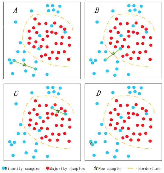
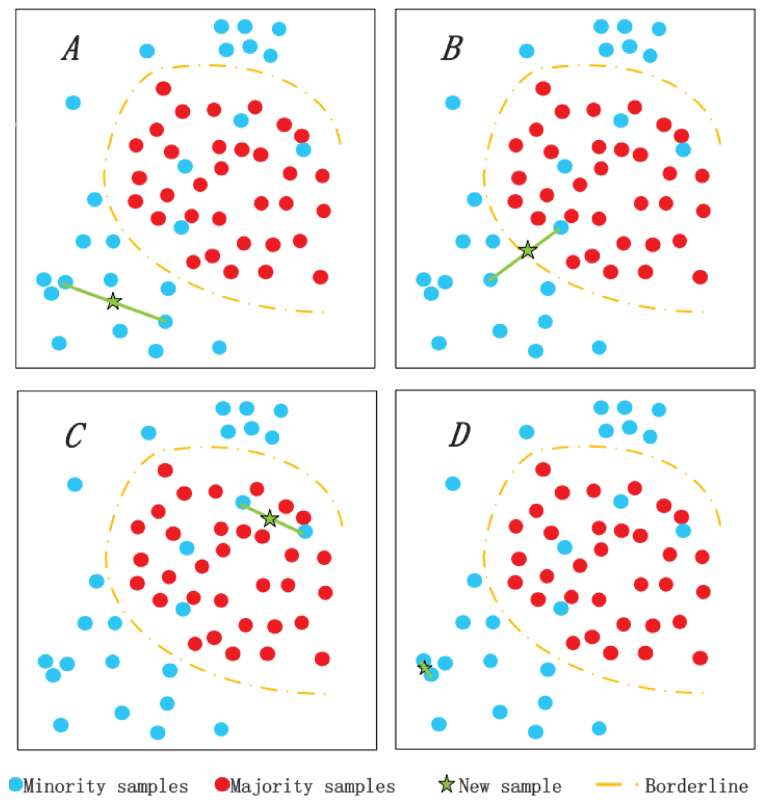
As one of the most effective approaches for addressing class imbalance, SMOTE has been widely applied. It synthesizes new minority samples by performing linear interpolation between existing minority samples, thereby balancing the class distribution and alleviating the class imbalance problem (see Figure 1A). Despite its simplicity and effectiveness, SMOTE still suffers from notable limitations (see Figure 1B–D).
Figure 1.
Major issues of SMOTE: The minority samples in majority regions are usually referred to as noise samples. Case (A) provides the sample synthesized by the SMOTE method under ideal conditions, where the new samples are located in the minority region. Cases (B,C) show noise samples that are precisely selected to participate in the synthesis. Case (B) leads to blurry boundaries, while case (C) results in the synthetic noise points. Case (D): Two minority samples participating in the synthesis are coincidence or particularly close. Although the samples are indeed synthesized in minority regions, it just brings duplicate information and might lead to overfitting.
Some recent SMOTE variants, such as KMeans–SMOTE and Density–SMOTE, have improved the performance of SMOTE to some extent, yet they still exhibit certain drawbacks. KMeans–SMOTE is highly sensitive to clustering quality, and noisy samples within the minority class can severely disrupt the clustering process [22]. Meanwhile, Density–SMOTE relies heavily on local density estimation; in regions with abrupt density variations, it may misjudge sample importance, leading to imbalanced sampling. Moreover, as data dimensionality increases, the accuracy of local density estimation deteriorates significantly, often resulting in overlapping synthetic samples near class boundaries.
To address the aforementioned limitations of SMOTE and its variants, we propose several improvements and introduce the following optimization strategies.
Firstly, PCA technology [23,24] is employed to reduce the dimensionality of the initial sample feature to three-dimensional space. Based on the distribution of the reduced-dimensional samples, the study selects symmetrical cubes with appropriate side length and arranges them closely together. In this way, the sample after dimensionality reduction will fall into only one cube. Then, samples are dynamically selected according to the established symmetrical cube scoring mechanism. Finally, the high-dimensional samples corresponding to the selected three-dimensional samples are found, which will be used to participate in the synthesis of minority samples. Since there are limitations on the side length of the cube, the CS-SMOTE method can effectively reduce the possibility of synthesizing noisy samples. In addition, CS-SMOTE simultaneously selects several samples to synthesize a novel sample, rather than using the linear interpolation of two samples in SMOTE.
The advantages of this approach are as follows. It eliminates reliance on K-nearest neighbors [25], and the constrained region size effectively reduces the generation of noisy synthetic samples. It enables the adaptive synthesis of varying numbers of new samples according to the local density of minority-class instances. It allows multiple existing samples to be jointly used for synthesizing each new sample, rather than being limited to interpolation between only two samples. During region construction, information from all available samples is leveraged to dynamically select appropriate points for synthesis, thereby achieving effective data augmentation and mitigating the impact of noise in the original dataset.
Numerical experiments on thirty-three datasets are carried out, which can be downloaded at https://sci2s.ugr.es/keel/imbalanced.php, accessed on 3 July 2025. The experimental results indicate that, compared with the conventional SMOTE and other improved SMOTE methods, the network model trained using samples synthesized by CS-SMOTE has better classification performance. Beside, to prevent accidental occurrence of only one classifier, the study tested the performances of each oversampling method on three usual classifiers: support vector machine (SVM) [26], extreme learning machine (ELM) [27], and multilayer perceptron (MLP) [28]. Therefore, CS-SMOTE can be effectively applied to solve class-imbalanced problems.
The rest of this paper is arranged as follows. In the next section, some related work is briefly introduced. A detailed description of the CS-SMOTE method is presented in Section 3. In Section 4, numerical simulations and the corresponding analysis are carried out. Some conclusions are drawn in Section 5.
2. Related Works
In this section, relevant work on dealing with class-imbalanced problems is briefly reviewed. These methods are basically address two aspects: algorithm improvement and data preprocessing. At the algorithm improvement level, an effective method for addressing class-imbalanced problems is cost-sensitive learning algorithms [29,30,31]. Data preprocessing involves manually generating minority samples (or deleting majority samples) to make the number of different classes approximately equal.
2.1. Algorithm Improvement (Cost-Sensitive Learning)
As one of the most effective methods in algorithm improvement, the classifier of cost-sensitive learning adopts the principle of minimizing expected costs for classification. The expected cost that a tested sample x is classified into the i-th class is as follows:
where denotes the posterior probability (or true risk) that sample x actually belongs to j-th class and represents the cost incurred when a sample truly belonging to j-th class is misclassified as i-th class.
Taking the binary classification problem as an example, the study uses 1 to represent positive classes and 0 to represent negative classes. The cost matrix for misclassification is as follows (see Table 1):
Table 1.
Cost matrix for misclassification.
In this cost matrix, each entry denotes the cost of predicting a sample as i-th class when its true class is j. and are the costs of correct classifications (often set to 0 or a small value). is the cost of a false negative—failing to detect a positive instance (e.g., missing a disease diagnosis). is the cost of a false positive—incorrectly labeling a negative instance as positive (e.g., unnecessary alarm or treatment).
In many real-world applications (e.g., medical diagnosis or fraud detection), false negatives or false positives may carry significantly higher costs than correct predictions, and cost-sensitive learning explicitly accounts for these asymmetric consequences during model training and decision-making.
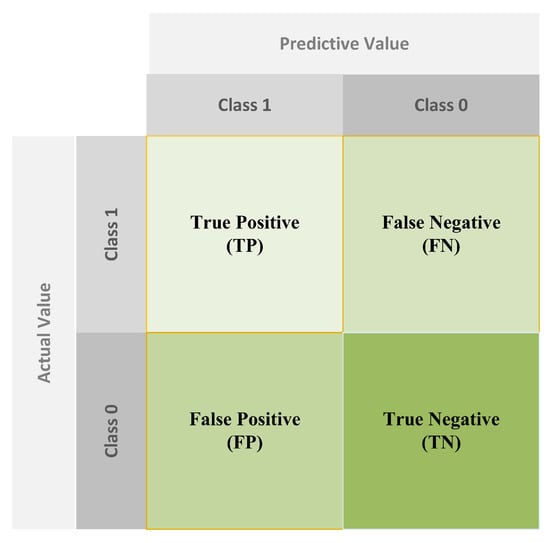
Here, the first number represents the predicted class, while the second number represents the actual class. Then, for a binary classification problem, the confusion matrix of classification results is as follows:
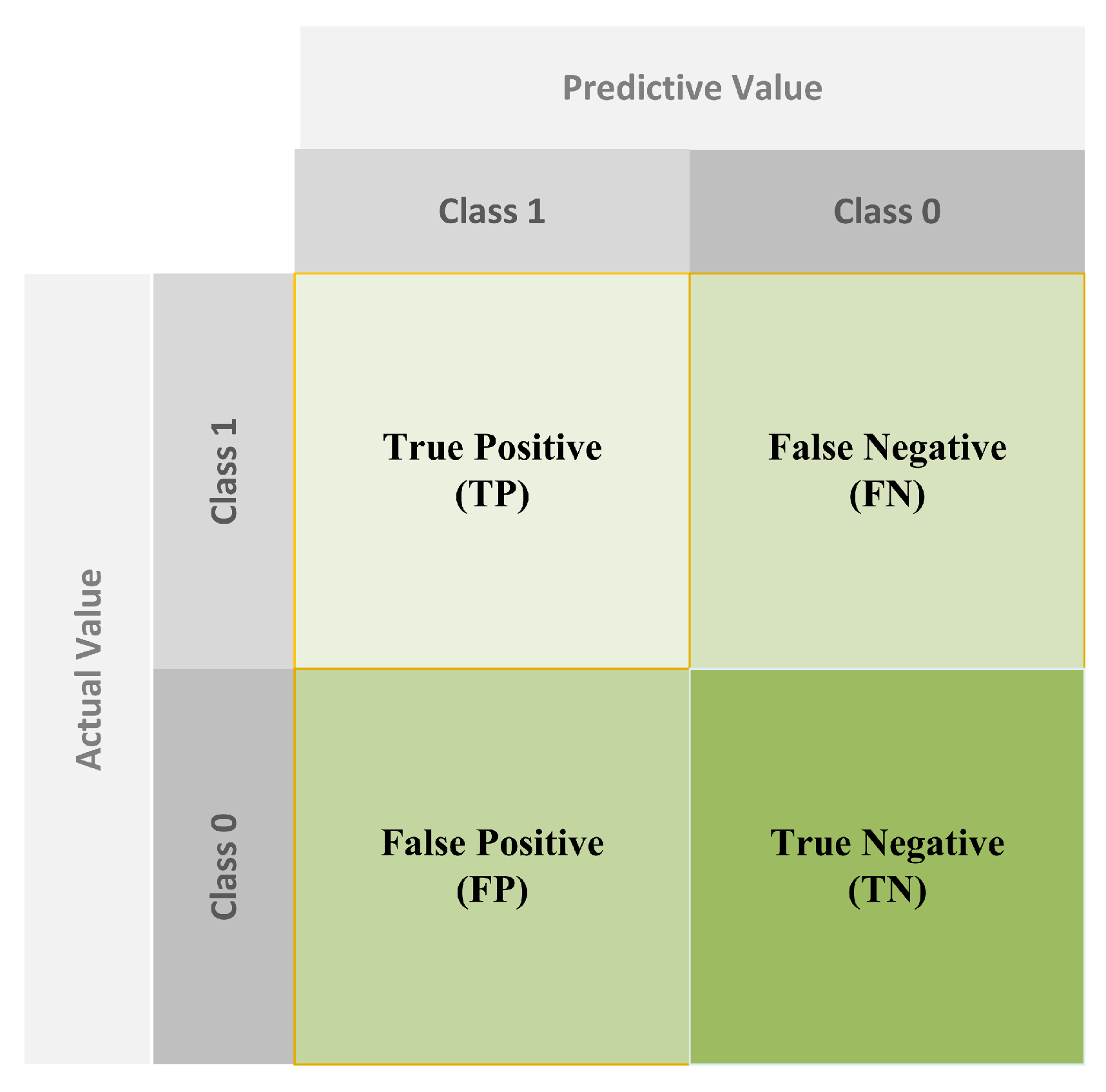
The confusion matrix summarizes the performance of a binary classifier by cross-tabulating actual and predicted labels. It contains four key components: True Positives (TP)—instances correctly predicted as positive (actual = 1; predicted = 1); False Negatives (FN)—positive instances incorrectly predicted as negative (actual = 1; predicted = 0); False Positives (FP)—negative instances incorrectly predicted as positive (actual = 0; predicted = 1); True Negatives (TN)—instances correctly predicted as negative (actual = 0; predicted = 0).
These counts directly correspond to the entries in the cost matrix; for example, FN relates to the cost and FP relates to . Understanding the confusion matrix (see Figure 2) is essential for evaluating classifier behavior—especially in cost-sensitive settings where the consequences of FP and FN errors differ significantly.
Figure 2.
Confusion matrix.
Therefore, the total cost of misclassification (TCM) [32,33] is as follows:
This equation quantifies the overall penalty incurred by a classifier due to incorrect predictions, weighted by the respective misclassification costs.
The direct cost-sensitive learning algorithm directly embeds the total misclassification cost of the classifier as the learning and optimization target into the learning process, so that the classifier has the property of cost sensitivity. The meta-learning algorithm for threshold adjustment converts cost insensitive classifiers into cost-sensitive classifiers by adjusting the discriminant threshold of the classifier.
The re-balanced meta-learning algorithm transforms cost-insensitive classifiers into cost-sensitive classifiers by re-balancing the total misclassification cost of different classes in the training sample set. The re-balancing ratio of positive and negative samples is as follows:
Through the above-outlined introduction to cost-sensitive learning algorithms, it is obvious that the improvements at the algorithm level are not intuitive enough. Next, let us take a look at the methods at the data preprocessing level.
2.2. Data Preprocessing
In cost-sensitive learning, classification decisions are guided by minimizing the expected misclassification cost rather than simply reducing error counts. This is particularly relevant in imbalanced scenarios where the consequences of misclassifying minority (e.g., positive) instances are far more severe than doing so for majority instances.
2.2.1. Undersampling and Oversampling
From the perspective of data preprocessing, a widely adopted strategy for handling class imbalance is resampling. The core idea is to adjust the class distribution so that classes with significantly different sample sizes become approximately balanced. Resampling methods fall into two main categories: undersampling and oversampling.
Undersampling achieves class balance by removing samples from the majority class. Common techniques include Random Undersampling (RUS) [34] and Focused Undersampling (FUS). While effective in reducing computational load and balancing class ratios, undersampling inevitably discards potentially useful information from the original dataset, which may lead to insufficient model training and loss of important decision boundaries.
In contrast, oversampling increases the number of minority-class samples to match the majority class, thereby preserving all original data. The simplest approach is Random Oversampling (ROS) [35,36], which duplicates existing minority samples to achieve balance. However, ROS often causes overfitting, as the model repeatedly sees identical instances, impairing its generalization ability.
2.2.2. SMOTE and Its Variants
To address the overfitting issue of ROS, the synthetic minority oversampling technique (SMOTE) has become the dominant oversampling method. SMOTE generates new synthetic minority samples by interpolating between existing minority instances and their nearest neighbors. Specifically, for each minority sample x, it identifies k nearest neighbors , randomly selects one neighbor , and creates a new sample along the line segment between x and :
This expands the minority class in the feature space, enabling the model to learn richer and more robust decision boundaries.
Building on SMOTE, several improved variants have been proposed:
Borderline–SMOTE [37,38] focuses on synthesizing samples near the decision boundary, where minority instances are most prone to misclassification, thereby enhancing boundary discrimination.
ADASYN (Adaptive Synthetic Sampling) [39] adaptively allocates more synthetic samples to minority regions with lower density, using local distribution as a weighting criterion. However, ADASYN does not account for correlations among minority samples and may introduce significant errors due to insufficient feature utilization.
Geometric–SMOTE (G-SMOTE) [40,41] defines a geometric region (e.g., a hyper-sphere or -cube) around each minority sample and synthesizes new points within this space. While innovative, G-SMOTE considers only minority samples and neglects the influence of majority-class and noisy samples.
KMeans–SMOTE [42] integrates clustering into the oversampling process. It first applies K-means clustering to the minority class and then performs SMOTE within each cluster to encourage more structured synthesis. However, this approach is highly sensitive to clustering quality; the presence of noisy or outlier samples in the minority class can severely disrupt the clustering process, leading to synthetic samples being generated in inappropriate regions.
Density–SMOTE [43] guides sample synthesis based on local density estimates of the minority class. It aims to generate more samples in sparse regions and fewer in dense ones to better reflect the underlying data distribution. Nevertheless, Density–SMOTE relies heavily on accurate local density estimation. In regions with abrupt density variations, it may misjudge the importance of certain samples, resulting in imbalanced or misleading synthesis. Moreover, as data dimensionality increases, the reliability of local density estimation deteriorates significantly, often causing synthetic samples to crowd or overlap near class boundaries—potentially harming classifier performance.
2.2.3. Limitations of Existing Methods
Despite these advances, current SMOTE-based methods still suffer from notable drawbacks. Most fail in the following areas:
- (1)
- Over-reliance on k-nearest neighbors: Most variants depend heavily on k-NN to define neighborhoods for synthesis [25], which is highly sensitive to noise and class overlap, often resulting in synthetic samples generated in ambiguous or misleading regions.
- (2)
- Restrictive interpolation mechanism: New samples are typically created by linear interpolation between only two points—the original minority sample and a single neighbor—failing to exploit richer contextual information from multiple surrounding instances.
- (3)
- Neglect of global class structure: Few methods account for the distributional relationships among all classes (both majority and minority), leading to synthetic samples that may distort true decision boundaries or exacerbate inter-class confusion.
- (4)
- Lack of adaptive synthesis control: Most approaches do not adjust the number of generated samples according to the local density of minority instances, causing either insufficient augmentation in sparse regions or excessive replication in dense areas.
- (5)
- Inadequate noise handling: During region construction, the synthesis process rarely leverages information from the full dataset to identify and suppress noisy or outlier minority samples, which can propagate errors and degrade model robustness.
To present a clearer comparison, we use Table 2 to contrast the aforementioned methods with the CS-SMOTE method.
Table 2.
Analytical comparison of SMOTE variants.
2.2.4. Summary and Motivation
To address these limitations, this paper proposes an improved SMOTE method based on a Cube Scoring mechanism (CS-SMOTE). CS-SMOTE is designed to minimize the generation of synthetic samples in noisy regions while explicitly considering the spatial distribution and inter-class relationships of all samples. This leads to higher-quality synthetic data and improved classifier robustness in imbalanced learning scenarios.
3. Proposed Improvement Method
3.1. Improvement Method
Several oversampling methods have been introduced in the previous section, especially the conventional SMOTE method. The drawback of the SMOTE method is that the samples involved in the synthesis are randomly selected with equal probability, which will lead to many noise points being synthesized in some special cases. In addition, SMOTE has issues with sample overlap and overgeneralization, which can quickly result in the expansion of the original noise samples. In order to address these shortcomings, some improved SMOTE methods have been proposed, such as MWSMOTE [44] and G-SMOTE. However, these methods also have their own limitations. This paper proposes the CS-SMOTE method, which is a multiple interpolation oversampling method based on a symmetrical cube scoring mechanism. The reason for reducing the dimensionality to 3D using PCA is that higher dimensions make it difficult to intuitively illustrate relevant concepts and produce visualizations, whereas 3D preserves more useful information compared to 2D. The detailed process of CS-SMOTE is as follows.
Step 1. Map the high-dimensional data dimensionality reduction to three-dimensional space.
First, PCA technology is applied to reduce all data features to three-dimensional space.
We primarily employ the commonly used Principal Component Analysis (PCA) method, which transforms the data into a new coordinate system through a linear transformation. It retains the most critical information by preserving the directions of maximum variance in the dataset. The core objective of PCA is to achieve dimensionality reduction while preserving as much of the essential data structure and information as possible.
To minimize the information loss caused by PCA, the transformed data are used only for sample selection. From this perspective, PCA can also help mitigate noise to some extent. Ultimately, the generation of new synthetic samples is performed in the original high-dimensional feature space.
Step 2. Overspread the entire three-dimensional space with cubes.
As is well known, countless adjacent cubes can cover the entire three-dimensional space. Therefore, the three-dimensional space is partitioned into identical cubes, and the dimensionality-reduced data obtained in Step 1 falls into exactly one cube. However, for different datasets, the distances between data points are diverse, which makes it impossible to select a fixed-size cube. The current problem is how long the side length of the cube should be for a certain dataset. Next, the selection of an appropriate cube size is introduced by defining four distances:
- : the average distance from each minority sample to other minority samples.
- : the average minimum distance from each minority sample to other minority samples.
- : the average distance from each sample to other samples.
- : the average minimum distance from each sample to other samples.
The specific mathematical calculation formulas are as follows:
where represents the i-th minority sample, is the i-th sample, and n and N represent the number of minority samples and the whole samples, respectively. Here, represents the minimum function and refers to the distance between two points A and B. With the above-outlined distance definitions, the proposed method can provide a method for calculating the edge length of the cube in three-dimensional space; that is,
Here, a is an adjustable parameter, satisfying the following inequality:
Formulas (6)–(8) provide an appropriate value for the edge length in the cube, with clear upper and lower bounds. In this algorithm, the upper bound in inequality (8) ensures that the cube is not too large, resulting in too many points being in one cube; on the other hand, the lower bound in inequality (8) ensures that the cube is not too small, which may result in too many cubes without sample points.
Step 3. Assimilate rules.
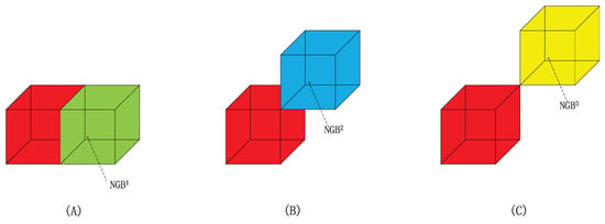
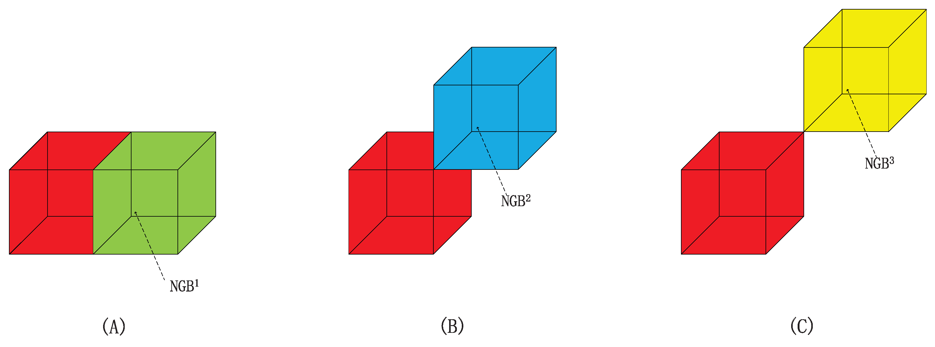
In three-dimensional space, each cube has 26 neighbors (NGB). Specifically, there are six co-planar neighbors, which are called first-type neighbors () in this paper; there are twelve co-linear neighbors, called second-type neighbors (); and there are eight co-vertex neighbors, named third-type neighbors (). Figure 3 shows three types of neighbor diagrams for a certain cube. It should be noted here that for a certain cube, the first type is closest and the third type is farthest. For the three figures in Figure 3, all of them possess symmetry and exhibit different symmetry manners with the red cube as the center. Specifically, Figure 3A shows the neighboring cubes co-planar with the red cube; if all the green neighboring cubes are depicted, there are 6 in total. Obviously, these 6 co-planar adjacent cubes are symmetrically distributed around the red cube as the center. Figure 3B and Figure 3C, respectively, show the co-linear neighbors and co-vertex neighbors of the red center cube. There are 12 co-linear neighbors and 8 co-vertex neighbors, respectively. If these neighbors are drawn in their entirety, then they are also symmetrical. The symmetry of these three types of neighbors gradually changes and they are different from each other.
Figure 3.
Three types of neighbor diagrams for a certain cube (red color). Green cube in (A) represents , blue cube in (B) belongs to , and yellow cube in (C) belongs to .
Next, the following part will introduce the meanings of several symbols:
- C: Each cube is recorded as an area C.
- : Co-planar, co-linear, or co-vertex cubes with C, called neighbors of C.
- : Co-planar cubes with C, called first-type neighbors of C.
- : Co-linear cubes with C, called second-type neighbors of C.
- : Co-vertex cubes with C, called third-type neighbors of C.
- : A cube only containing minority samples.
- : A cube only containing majority samples.
- : A cube without any samples.
- : A cube that contains both minority and majority samples is denoted by the confusing area . The confusing area is distributed at the boundary under normal conditions.
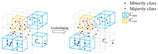
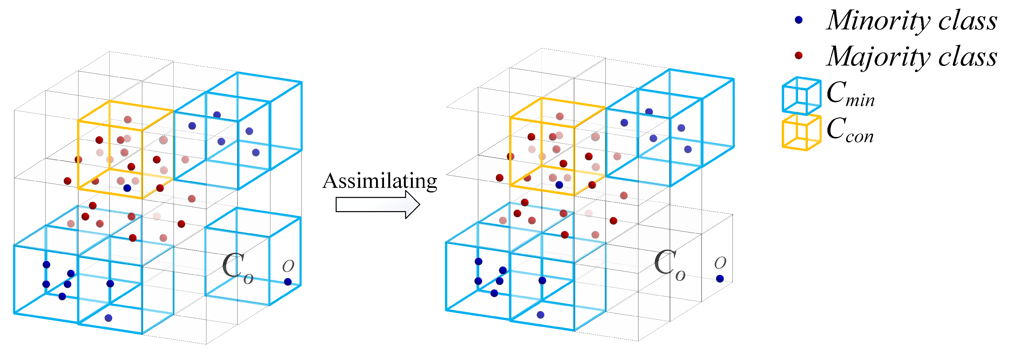
Finally, the following section introduces the assimilation rules. For a cube (), if all its twenty-six neighbors are (), then the cube C will be assimilated into . If the neighbors of C belong to different types of areas or some of these neighbors belong to , then C will not be assimilated. As shown in Figure 4, there is only one minority sample in cube , i.e., . Then, since all neighbors of belong to , the cube is assimilated into . Take cube as an example; if all its neighbors belong to , then will be assimilated into . Therefore, the minority samples in can be regarded as noise samples and not be selected to participate in the synthesis.
Figure 4.
Diagrams of naming and assimilation. When naming, the cube (blue cube), and all its neighbors ; so after assimilation.
Step 4. Establish scoring rules and select samples to participate in synthesis.
Before assimilation, only and areas have the minority samples. However, some of and areas will be assimilated into or , and the minority samples in these areas will not be selected to synthesize. Therefore, the minority samples in and areas after assimilation participate in the synthesis. These areas were assimilated only for the purpose of participating in scoring and weighting, and the classes of the samples in these areas are not changed. Then, the proposed method scores different areas and assigns the weights. A higher scoring area means that the corresponding weight will be greater. Finally, the selection probability is determined according to the weights. Specifically, for an area that can participate in the synthesis, the scoring rules are as follows:
- (1)
- The score of area consists of four parts: the score of itself and the scores of its three types of neighbors. Set the score of itself as . For the six first neighbors , the proposed method labels them as (), and the corresponding scores are denoted as . The naming rules of the other two types are similar, with the .
- (2)
- If , then .
- (3)
- If , then .
- (4)
- If , then , .
- (5)
- If , then , .
- (6)
- If , then , .
- (7)
- If , then , .
- (8)
- If , then , .
- (9)
- If , then , .
- (10)
- If the neighbor belongs to , the corresponding score is 0.
For two neighbors of , their contributions to the score of depend on both their spatial relationship and their class membership. If both neighbors belong to the same class, either or , the one that is spatially closer to receives a higher score. Moreover, when comparing neighbors with the same spatial relationship, a neighbor from contributes more to the score of than a neighbor from .
In addition to distance and class type, the type of geometric adjacency also affects the scoring. Specifically, among all neighboring cubes, those that share a face, also referred to as coplanar neighbors, with are considered the closest and thus earn the highest scores. Neighbors that share only an edge receive a lower score, and those that share only a vertex receive the lowest score among adjacent regions. This reflects the intuition that face-sharing neighbors exhibit stronger spatial correlation than edge-sharing or vertex-sharing neighbors.
Combining these principles, the scoring mechanism prioritizes neighbors that are geometrically proximate, where coplanar adjacency is scored higher than edge-sharing, and edge-sharing is scored higher than vertex-sharing. As a result, a coplanar neighbor from yields the highest possible contribution to the score of , while a vertex-sharing neighbor from contributes the least. This design ensures that sample synthesis focuses on regions that are both structurally cohesive and representative of the minority class.
With these scoring rules, the total score of cube can be calculated by
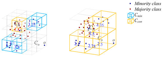
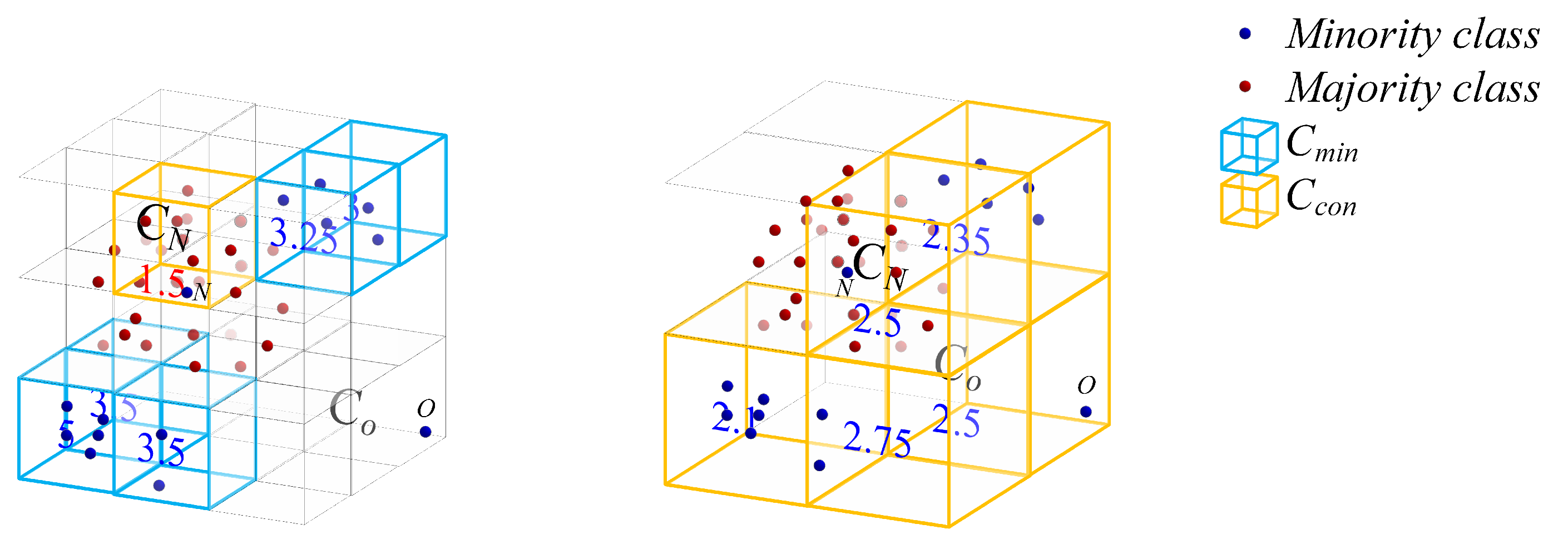
Under the scoring rules mentioned above, the proposed method can score all and areas. Figure 5 provides an example of the scoring method with different side lengths. Specifically, in the left figure, there are both minority and majority samples in . Thus, belongs to the confusing cube , and . As for the three types of the neighbors, only one belongs to , while the other twenty-five neighbors are either or . Therefore, the scores obtained by twenty-six neighbors of are as follows:
Figure 5.
The influence of side length selection on the cube . The numbers represent the total scores for all minority cubes and confusing cubes.
Finally, for the cube , the total score is . In the right figure of Figure 5, also belongs to the confusing cube . At this time, has four confusing neighbors: two and two . According to the scoring rules, . In summary, the position, size, samples, and score of the cube have changed under different side lengths.
However, there will definitely be some areas with low final scores. Then, CS-SMOTE determines that the weights of these areas are too small. In order to facilitate the subsequent synthesis of minority samples, we directly assign these areas a score of 0. Here, the proposed method takes a score of 1.5 as the measurement score. That is to say, if the score of an area is less than 1.5, then the samples in this area do not participate in the synthesis. Under this scoring mechanism, we can provide the score of each area, and the higher the score, the greater the possibility of ultimately selecting minority samples in this area for synthesis. Assuming that n, areas ultimately obtain scores, denoted as . The probability formula for selecting minority samples in the j-th area to participate in the synthesis is expressed as
Step 5. Synthesize novel minority samples.
The first area is selected based on the probability determined by Equation (10) in Step 4. To synthesize novel minority samples, it is necessary to select at least one more area. Next, the 26 neighbors of cube are examined. If at least one of belongs to or , then the area must contain minority samples that can participate in synthesis. It is assumed that the number of areas that meet the conditions is denoted by m. On the contrary, if none of can meet the conditions (with minority samples), then the cube will be abandoned.
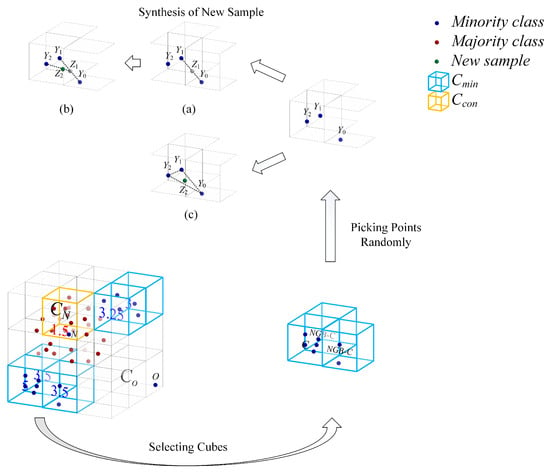
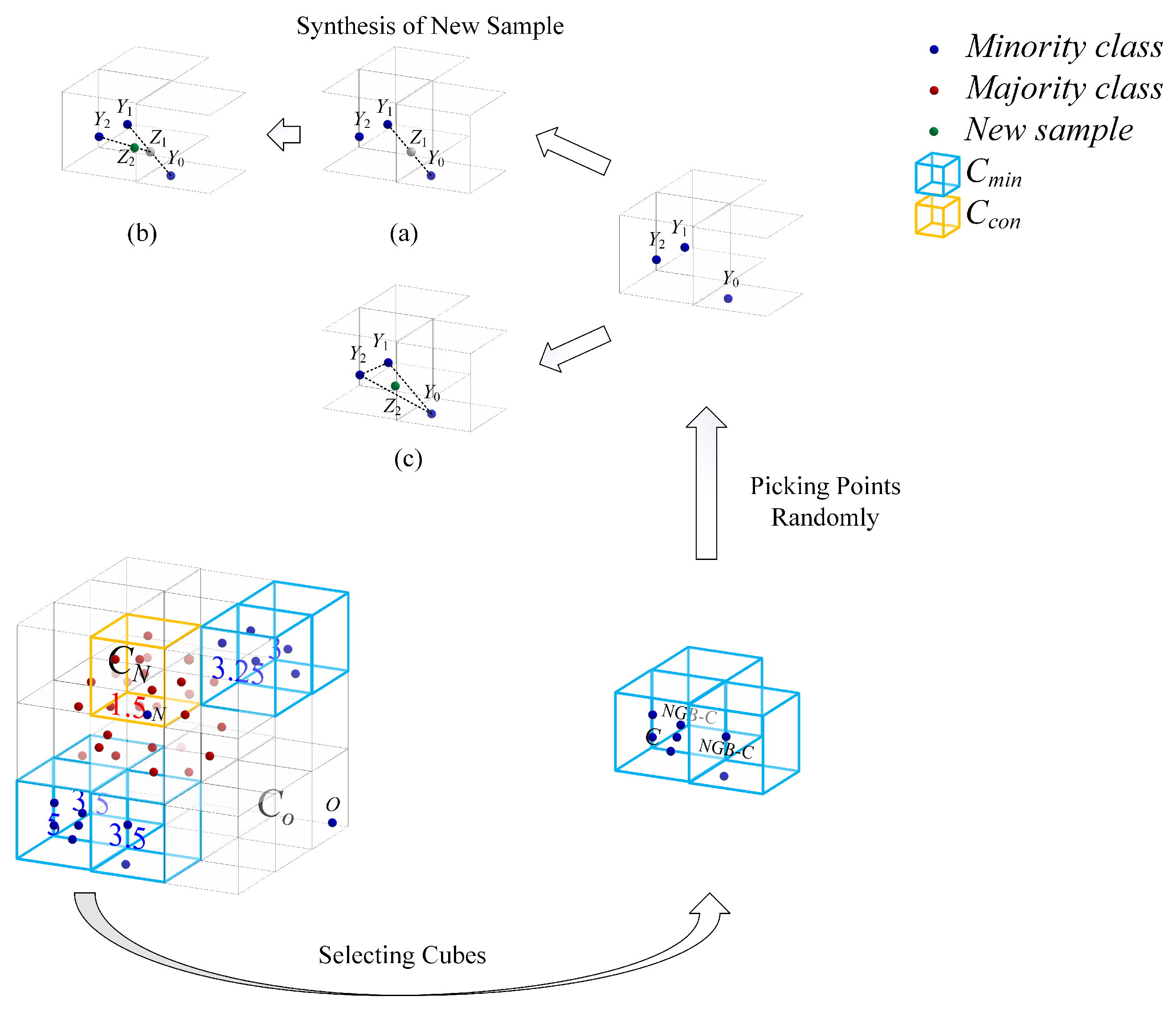
Next, CS-SMOTE will focus on synthesizing minority samples. As the first step, we randomly and equally select a minority sample from cube , denoted by ; in the second step, CS-SMOTE randomly selects one minority sample from each , denoted by . In the third step, the proposed method locates the high-dimensional samples corresponding to these three-dimensional samples, denoted by . Finally, in the fourth step, these high-dimensional samples are employed for multiple linear interpolation, and a novel minority sample can be synthesized. Specifically, let be random numbers ranging from 0 to 1, then the interpolation formulas are as follows:
The obtained is the final synthesized minority sample. Take a three-dimensional dataset as an example; Figure 6 shows the process diagram for the multiple interpolation of three points (, and ). Specifically, linear interpolation is applied to and to obtain . Similarly, we can obtain based on and . Obviously, will be located inside the triangle, surrounded by three points: , , and .
Figure 6.
Flow chart of sampling and synthesizing new sample. Blue points are minority samples, red points are majority samples, and green point is new synthesized sample. (a) is obtained through linear interpolation of and ; (b) is obtained through linear interpolation of and ; (c) The newly synthesized sample falls into the triangle surrounded by , and .
In summary, the cube scoring mechanism can select cubes based on probability and randomly select minority samples from neighbors, ultimately synthesizing samples from the original dimension. In addition, CS-SMOTE can prevent the interpolation of two samples that are too close to each other. Since the distance of the two samples is close, they will be allocated to the same cube. However, during the synthesis process, at most one sample is selected from each cube.
Step 6. Train the network based on the obtained class-balanced datasets.
In Step 5, this section has provided a detailed introduction on how to synthesize a minority sample. For a certain class-imbalanced dataset, as long as the class imbalance ratio is known, an appropriate number of minority samples is repeatedly synthesized until the dataset is balanced.
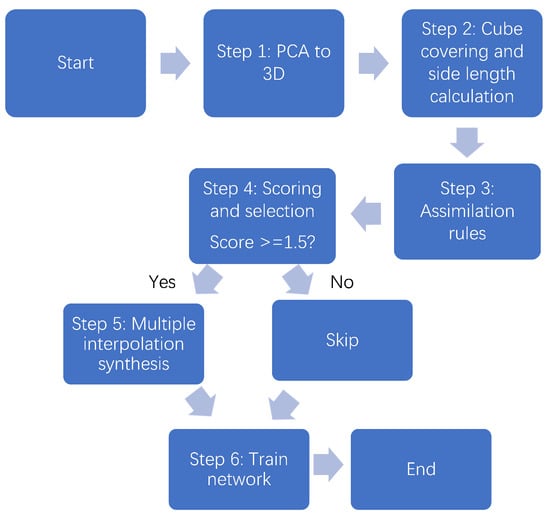
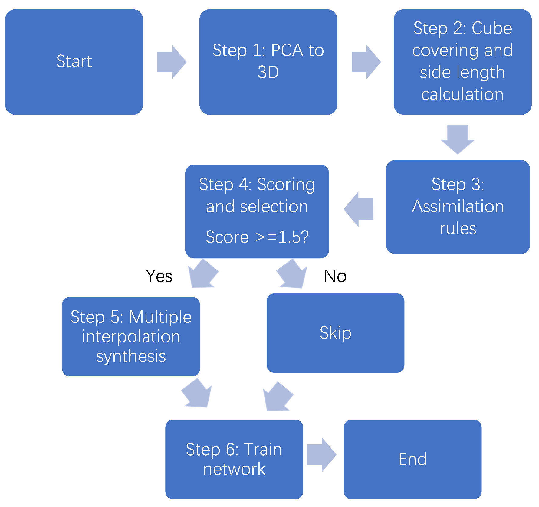
Figure 7 is a brief flowchart summarizing all the steps described above.
Figure 7.
A brief flowchart summarizing all the steps described above.
After obtaining the class-balanced dataset, it is crucial to evaluate the performance of the minority samples synthesized by CS-SMOTE method on various network models. In the subsequent numerical experiment part, we will train three networks under different oversampling methods, and compare the performance of these methods according to several indicators.
3.2. Computational Complexity Analysis
Factor a is an adaptive parameter that controls the side length of the cubic regions. We need to constrain the value of a within a reasonable range. If the side length is too small, a large number of minority-class regions will be filtered out, leaving almost no regions or samples available for synthesis. Conversely, if the side length is too large, the partitioning loses its meaning and becomes ineffective at filtering out noise.
Within this valid range, we investigate the optimal value of a from both performance and time complexity perspectives. Suppose the dataset contains n samples with an imbalance ratio of r. Assume that along the x, y, and z axes, there are i, j, and k cubic regions, respectively. Thus, the total number of cubic regions to be constructed is approximately .
Traditional SMOTE traverses all minority-class samples (whose number is ) and searches for the k-nearest neighbors of each minority sample among all samples, resulting in a time complexity of .
First, we employ PCA to formulate selection rules. Standard PCA requires full eigendecomposition of an matrix, which has a time complexity of . However, if the data are projected only onto the first q principal components, it suffices to compute the top q eigenvalues and eigenvectors, yielding a time complexity of . In our work, we reduce the dimensionality to three dimensions (), which is much smaller than n; hence, the PCA step in our algorithm can be considered to have a time complexity of .
Next, we consider the time complexity of generating the cubic regions. Approximately cubic regions are generated, with a time complexity of . Subsequently, operations such as assimilation, scoring, probability calculation, and sample synthesis are performed for each region. These operations involve traversing each region and its 26 neighboring regions, resulting in a time complexity of .
Finally, we consider the matching process between samples and regions. This step requires iterating over all samples and all regions, leading to a time complexity of .
In summary, the overall time complexity of our algorithm is
Therefore, we should choose a relatively large side length (i.e., a larger factor a) to ensure without compromising performance. Under this condition, the difference in time complexity between our algorithm and SMOTE is not significant. Based on this analysis, we conclude that, provided performance degradation is negligible, a larger value of factor a leads to lower time complexity.
3.3. The Performance Metrics and Basic Settings
To demonstrate the superiority of the CS-SMOTE, this paper compared it with the following commonly used oversampling methods: non-SMOTE, SMOTE, Borderline, ADASYN, G-SMOTE, MWMOTE, GAUSSIAN–SMOTE, DTO-SMOTE, and KNNOR. With the synthesized minority samples, the class-imbalanced problem is transformed into a regular binary classification problem. In our experiments, support vector machine (SVM), extreme learning machine (ELM) and multi-layer perceptron (MLP) networks are employed to detect whether the synthesized samples are reasonable under various methods.
In order to evaluate the performance of CS-SMOTE and other methods, this paper calculates several criteria. For a binary classification problem, the mathematical formulas of , , and [45] are
However, among the three evaluation indicators mentioned above, mainly leans towards the majority samples, while and only focus on the minority samples. Therefore, in order to evaluate the comprehensive classification ability, three additional indicators are employed to evaluate classification performance: F1-measure [46,47], G-mean [48], and area under curve (AUC) [49]. F1-measure is the weighted harmonic average of recall and precision, and G-mean is the weighted geometric average of recall and precision. The calculation methods for F1-measure and G-mean are as follows:
AUC is defined as the area enclosed by the ROC curve and the coordinate axis, which is evidence that the value of this area will not exceed 1. Since the fact that the ROC curve is generally above the line , the range of AUC values is between 0.5 and 1. The closer the AUC is to 1.0, the higher the authenticity of the detection method. When the AUC value is equal to 0.5, the authenticity is the lowest and has no application value.
For each class-imbalanced problem, a five-fold cross-validation technique [50,51] is applied. Specifically, the dataset is randomly divided into five parts, with equal or almost equal sample numbers. At each time, only one part is selected as the test sample, while the other four parts are the training samples. In this way, different parts are selected as the test sets and five results are obtained. Next, the above-outlined processes are repeated 20 times, yielding a total of 100 sets of experimental results. Finally, the average of these 100 result sets is used for subsequent comparison. Obviously, comparing the average values in experiments can avoid the possibility of particularly good or bad results in only one experiment, which will make the comparison results more convincing.
Finally, the process (see Algorithm 1) of the CS-SMOTE method is provided as follows:
| Algorithm 1 Oversampling method based on symmetrical cube scoring mechanism (CS-SMOTE). |
|
4. Experiment and Analysis
In this section, the advantages of the proposed CS-SMOTE method are demonstrated through experimental verification. The experimental settings are first introduced, including the datasets, classifiers, comparative methods, and related parameters. In next subsection, experimental results and corresponding analysis are presented.
4.1. Experiment Settings
This section mainly conducts the numerical experiments on thirty-three class-imbalanced problems, which are provided by the KEEL database. The specific information of these datasets are shown in Table 3.
Table 3.
Description of experimental datasets.
4.2. Experimental Results and Analysis
This section comprises three main subsections. Initially, this section provides the comparison and analysis of experimental results. Following this section, a data visualization is given to visually display the position of the synthesized samples. Lastly, the significance of the experimental results is assessed through statistical tests. Significantly, Borderline–SMOTE and Gaussian–SMOTE are denoted by Borderline and Gaussian in the tables.
4.2.1. Comparison and Analysis of Experimental Results
In this subsection, performance comparison results between the proposed CS-SMOTE method and eight other oversampling methods are presented. After obtaining a class-balanced dataset through different oversampling methods, the focus should be on evaluating which oversampling method performs better. In order to avoid the accidental phenomenon caused by using only one classifier, SVM, ELM, and MLP are employed to test the samples synthesized by these oversampling methods. These are three mainstream classifiers, which do not affect our subsequent evaluation; they merely serve as tools for generating the specific metric values. Table 4, Table 5, Table 6 are the performance comparison results of these oversampling methods on thirty-three datasets, of which three tables were trained under SVM, ELM, and MLP, respectively.
Table 4.
The result for mean cross-validation score of sampling across the dataset when using SVM as the classifier (The values marked in bold indicate that the corresponding method under this indicator is the best).
Table 5.
The result for mean cross-validation score of sampling across the dataset when using ELM as the classifier (The values marked in bold indicate that the corresponding method under this indicator is the best).
Table 6.
The result for mean cross-validation score of sampling across the dataset when using MLP as the classifier (The values marked in bold indicate that the corresponding method under this indicator is the best).
From Table 4, Table 5, Table 6, it can be observed that CS-SMOTE performs best more frequently than other oversampling methods. In a total of ninety-nine experiments with three classifiers and three estimators, the optimal performance numbers for F1-score, G-means, and AUC of CS-SMOTE are 61, 57, and 61, respectively. The results also indicate that the performance of the CS-SMOTE classifier with SVM is slightly better than the other two classifiers.
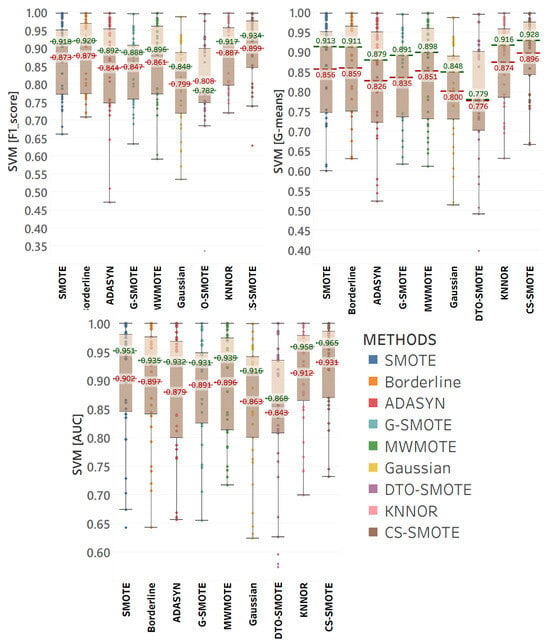
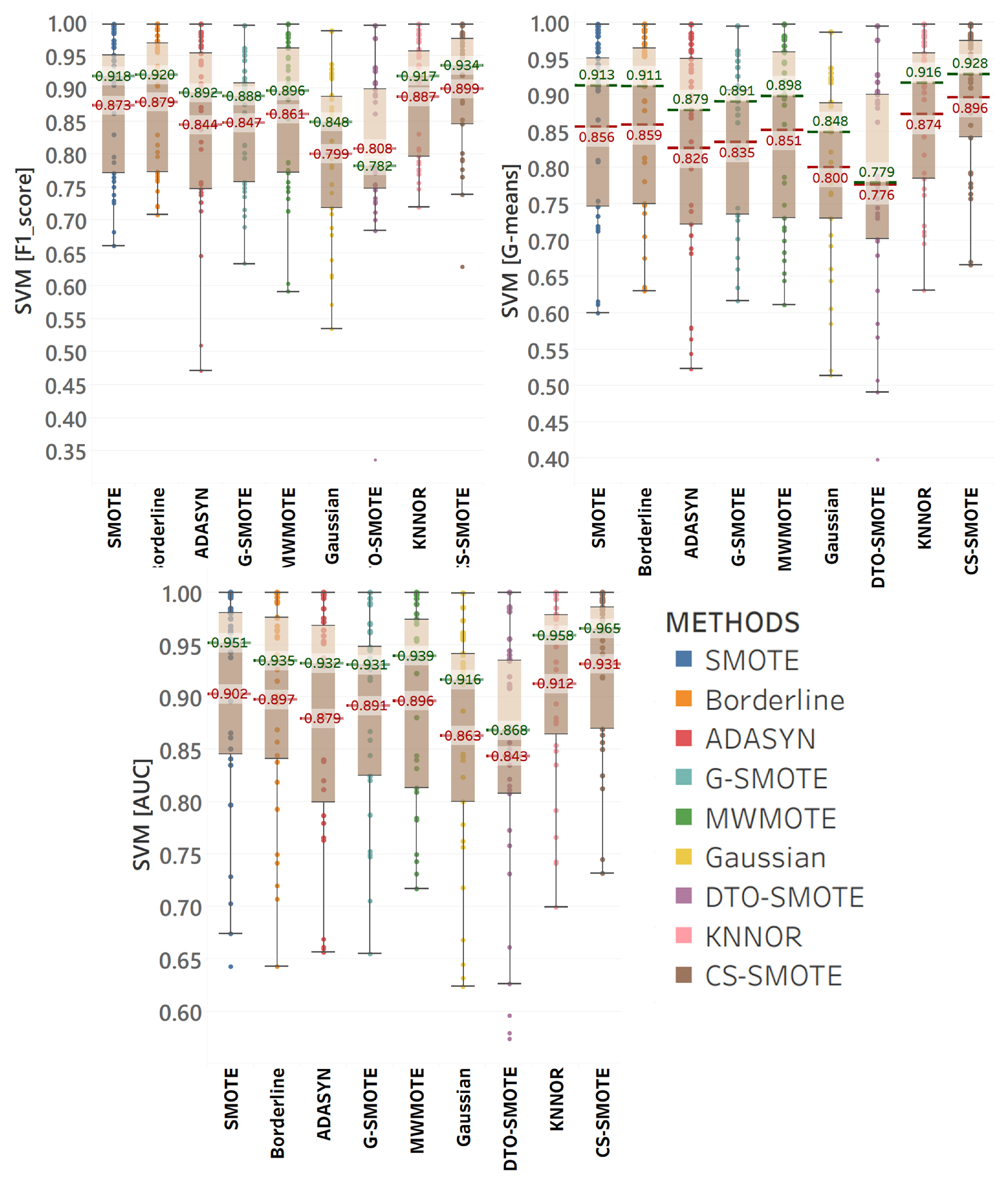
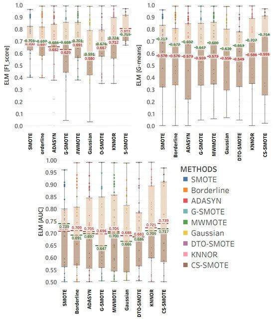
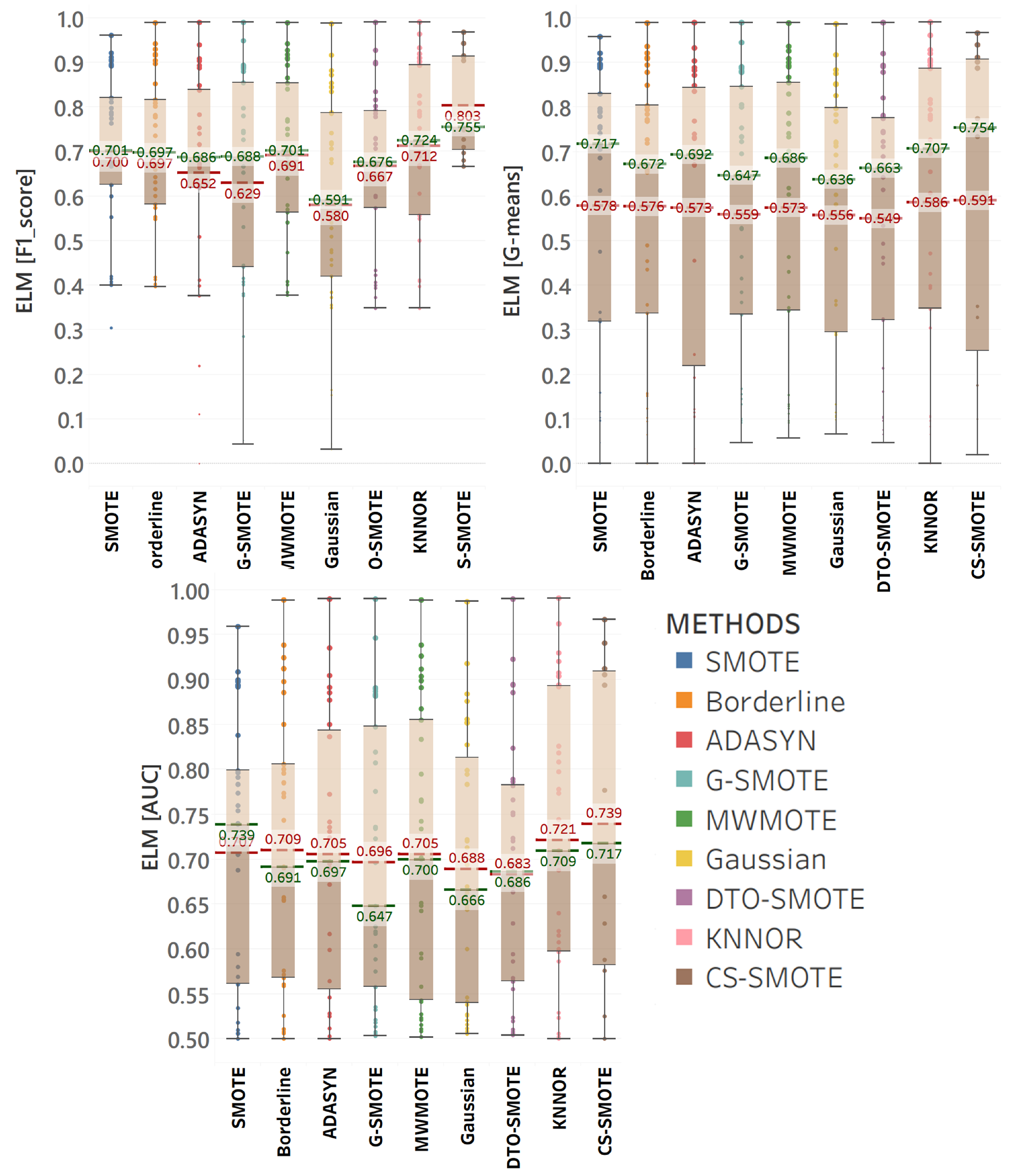
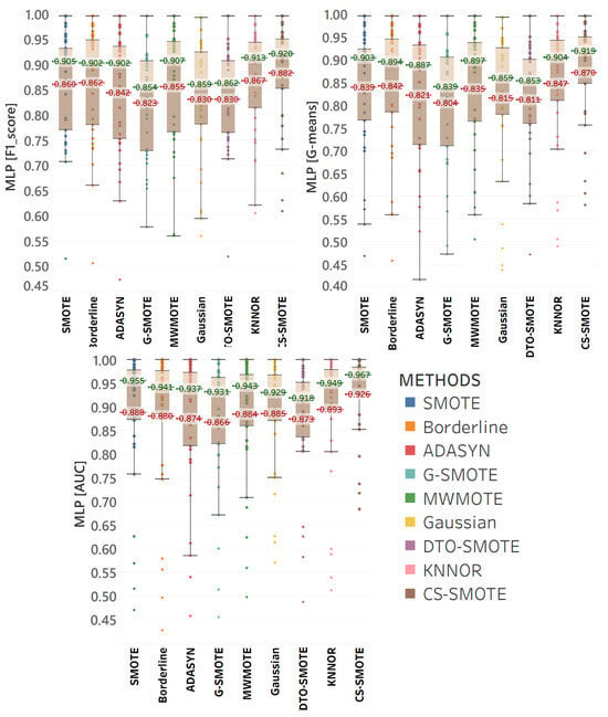
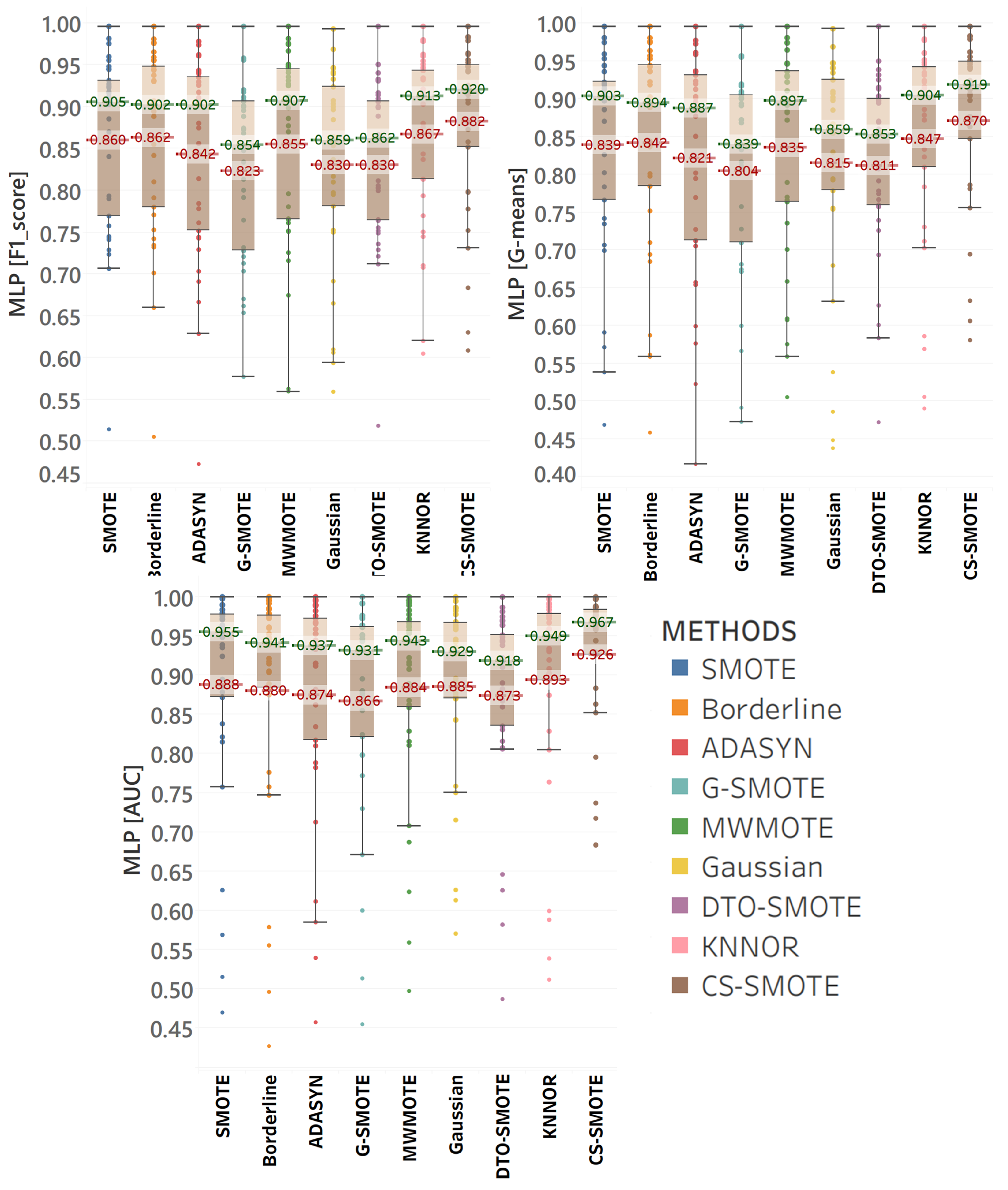
In addition, CS-SMOTE calculates the ranking of these oversampling methods under each evaluation estimator, and the mean ranking of thirty-three datasets is displayed in Table 7. It can be seen that regardless of which classifier was used, CS-SMOTE has the best rank in terms of classification performance. To more intuitively reflect the mean ranking, CS-SMOTE has also provided the ranking of three performance estimators (see Table 8). It is obvious that the top three oversampling methods are CS-SMOTE > KNNOR > Borderline. In order to more intuitively reflect the evaluation estimators, box charts have also been provided (as shown in Figure 8). Figure 8 demonstrates the comprehensive performance of different oversampling methods under three estimators in the SVM classifier. The solid line from top to bottom represents the maximum, upper quartile, median, lower quartile, and the minimum value of the result. Obviously, CS-SMOTE has the highest average value in each group. That is to say, the performance of CS-SMOTE is the best, and CS-SMOTE is usually superior to other oversampling methods. Figure 9 and Figure 10 provide box charts for ELM and MLP classifiers, respectively. While ELM is employed to measure the AUC performance, although the average value of CS-SMOTE is the best, the median value of CS-SMOTE is only slightly lower than that of SMOTE. Looking back at Table 8, the ranking of CS-SMOTE is , slightly better than the ranking of SMOTE , which means that CS-SMOTE is slightly better than SMOTE.
Table 7.
Results for mean ranking of different estimators across the dataset (The values marked in bold indicate that the corresponding method under this indicator is the best).
Table 8.
Results for mean ranking of different classifiers across the dataset (The values marked in bold indicate that the corresponding method under this indicator is the best).
Figure 8.
Box chart of results: This diagram shows the comprehensive performance of different oversampling methods under three estimators in SVM. The solid lines from top to bottom represent the maximum, upper quartile, median, lower quartile, and minimum values of the results, respectively. The green dashed line and number represent the median value of each group and the red dashed line and numbers represent the average value of each group. Some points are beyond the normal range and are usually considered as outliers.
Figure 9.
Box chart of results in ELM.
Figure 10.
Box chart of results MLP.
Finally, to demonstrate how much better CS-SMOTE is, CS-SMOTE provides a superior percentage improvement in performance estimators compared to other methods (see Table 9). The larger the value, the greater the difference between CS-SMOTE and this method. Obviously, all of the values are greater than 0, which means CS-SMOTE is the best among all of these nine oversampling methods.
Table 9.
Results for mean percentage difference between CS-SMOTE and the rest of the main samplers.
4.2.2. Data Visualization
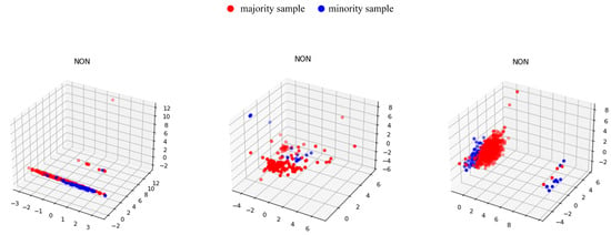
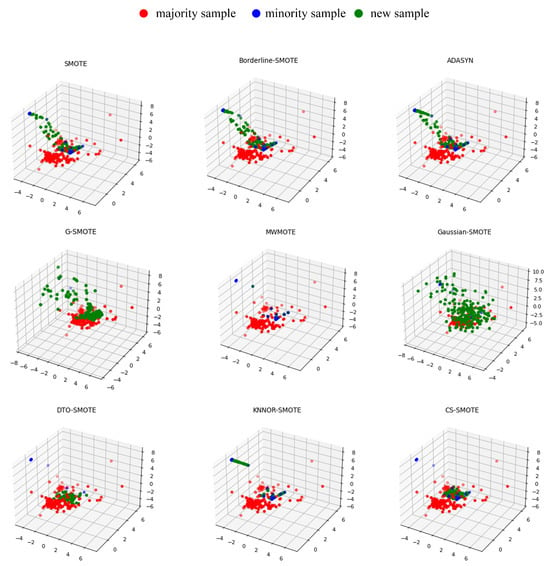
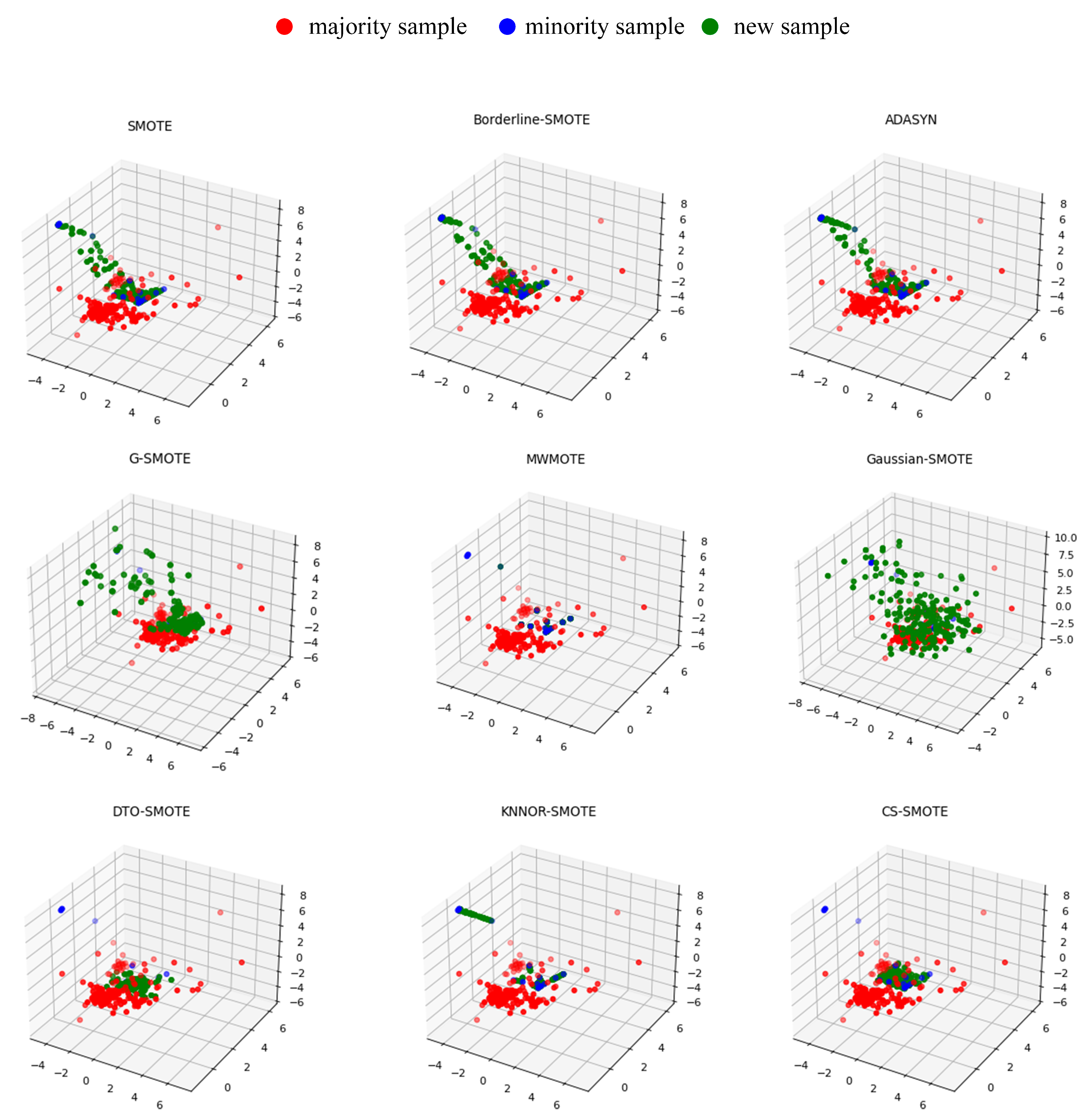
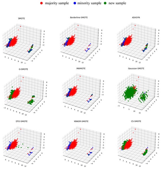
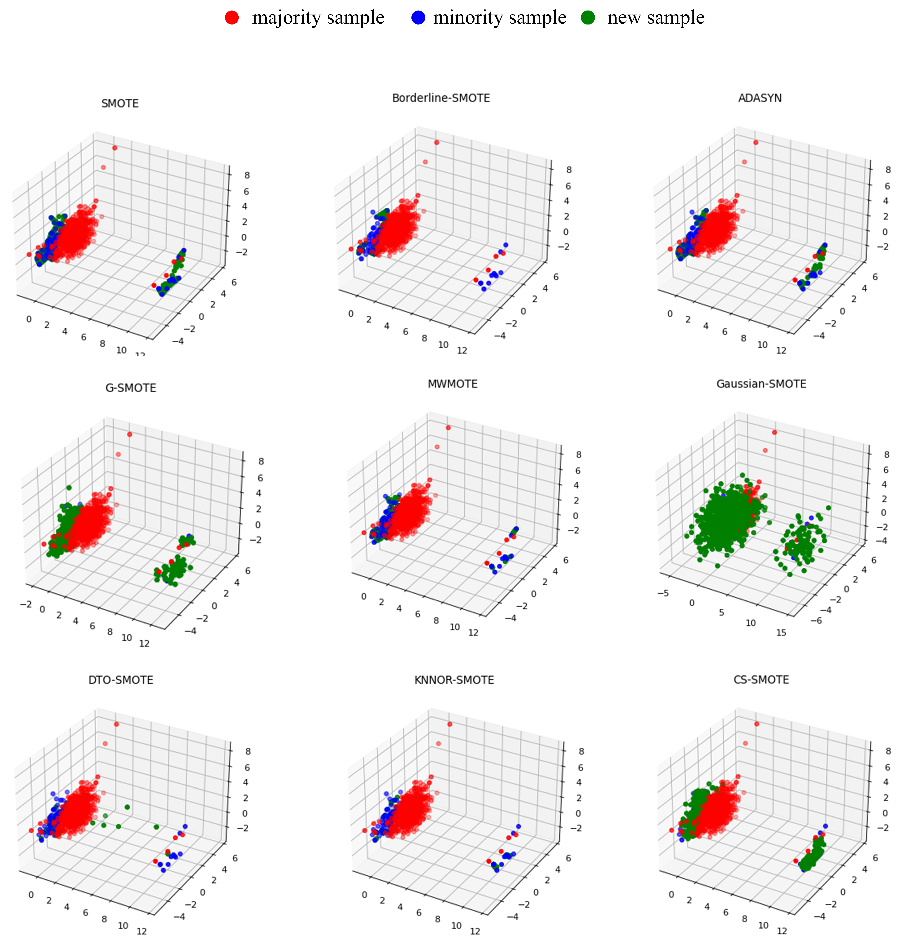
To visually display the position of the synthesized sample, the proposed method chooses ecoli_ 0_ 1_ 4_ 6_ Vs _ 5, Glass4, and Yeast_ 0_ 2_ 5_ 7_ 9_ Vs_ 3_ 6_ 8, three datasets to illustrate the synthesis results of different oversampling methods in a three-dimensional plane. The visualizations of these three datasets without oversampling are shown in Figure 11.
Figure 11.
The visualizations of three datasets without oversampling.
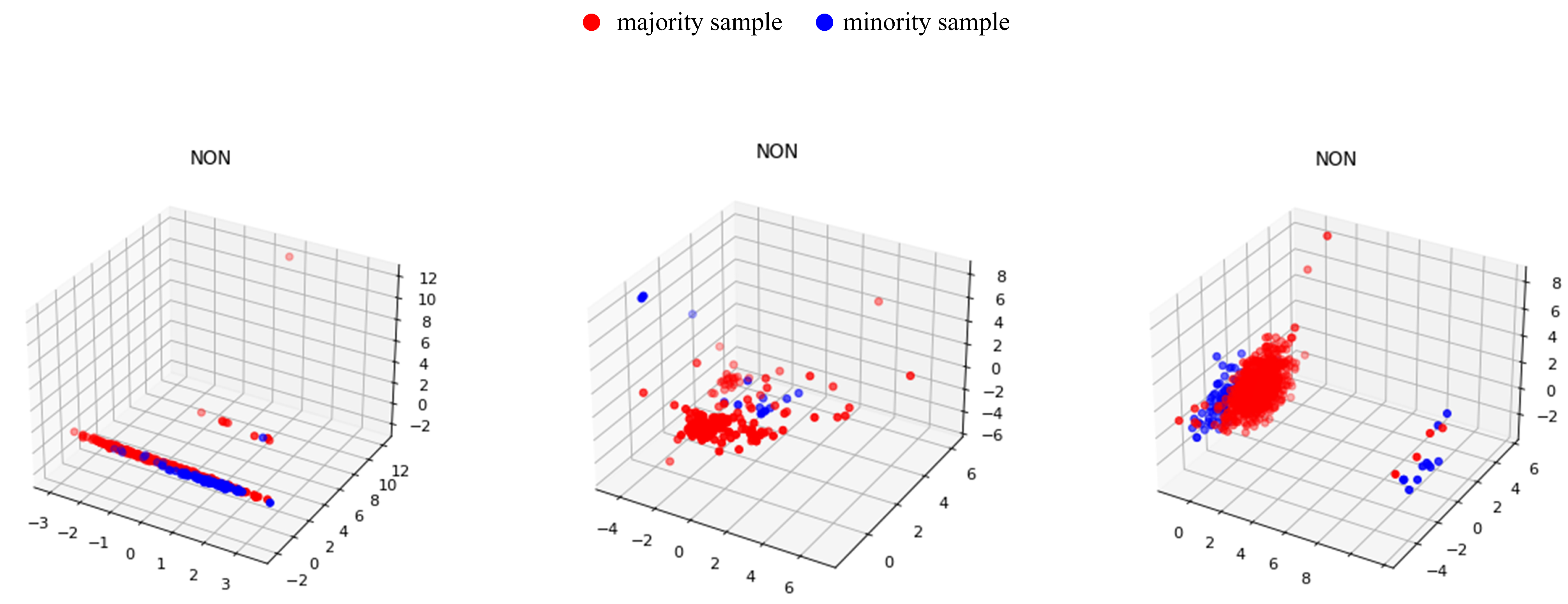
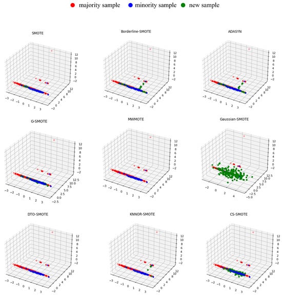
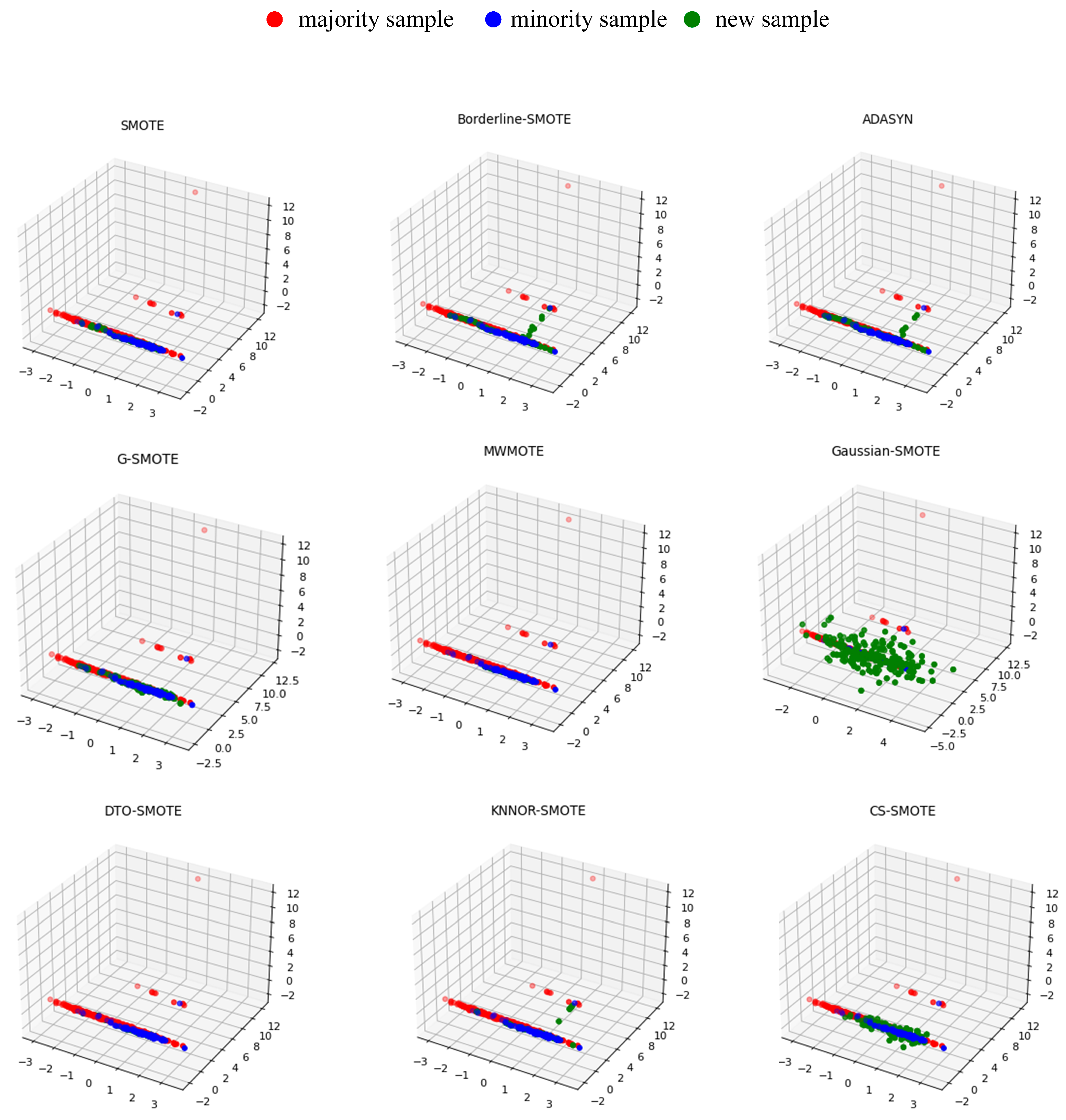
The distinctive styles employed by various sampling methods are shown in Figure 12, Figure 13 and Figure 14. Specifically, SMOTE employs random sampling between neighbors, Borderline–SMOTE concentrates on generating boundary samples, and ADASYN generates additional samples in regions with low sample density. G-SMOTE distributes new samples in a region that is in proximity to the original ones, whereas DTO-SMOTE primarily generates samples in partitioned spaces. The new samples of Gaussian-SMOTE conform to a Gaussian distribution, while MWMOTE and KNNOR-SMOTE synthesize samples based on probability and rule selection between selected samples. Finally, CS-SMOTE filtered noise and outliers, and then applied multiple linear interpolations to generate new samples in the selected area.
Figure 12.
Samples synthesized through sampling ecoli_0_1_4_6_vs_5 dataset with nine methods.
Figure 13.
Samples synthesized through sampling glass4 dataset with nine methods.
Figure 14.
Samples synthesized through sampling yeast_0_2_5_7_9_vs_3_6_8 dataset with nine methods.
Compared to the geometric regions of G-SMOTE, the field of CS-SMOTE effectively filters out noise samples, resulting in a more concentrated generation of new samples. Additionally, while both CS-SMOTE and MWMOTE utilize clusters or fields to generate new samples, the multiple interpolations of CS-SMOTE between the field ensures that the samples would not only concentrate in a few clusters, thus enhancing sample diversity and fitting to the sample distribution.
Especially for Figure 12 and Figure 13, when the samples are scattered in a main region with outliers. SMOTE, Borderline–SMOTE, ADASYN, G-SMOTE, Guassian–SMOTE, and DTO-SMOTE generated a large quantity of noise between the region and outliers. Then, Figure 12, Figure 13 and Figure 14 show that Borderline–SMOTE, MWMOTE, and KNNOR-SMOTE only generated new samples in a small geometric area, which can easily cause overfitting. Additionally, Borderline–SMOTE only generated samples around the boundary, so it lost a lot of original distribution information. In contrast to these methods, CS-SMOTE ensures that the samples are not generated between outliers and regions, or between distinct regions. The practice has proved that CS-SMOTE can effectively solve the imbalanced classification of multiple regions and outliers.
4.2.3. Results of Statistical Tests
Table 10 and Table 11 show the results of the Frideman test and the Wilcoxon signed rank test, and all the test results met p-value . The result of Table 10 means that different sampling methods can be compared and the result of Table 11 indicates significant differences between CS-SMOTE and other sampling methods. Therefore, combined with statistical tests and experimental results analysis, CS-SMOTE has the best overall performances.
Table 10.
Results for Friedman test of different estimators.
Table 11.
Results for the Wilcoxon signed rank test.
5. Conclusions
The proposed CS-SMOTE method addresses class imbalance by reducing noise in synthetic samples. After PCA-based dimensionality reduction, it introduces a symmetric cube scoring mechanism in 3D space to select regions for synthesis, then generates new minority samples via multi-point linear interpolation in the original feature space.
A key strength is the elimination of K-nearest neighbor dependency. Synthesis is guided by global sample distribution rather than local neighborhoods, and the number of new samples adapts to local minority density. Each synthetic instance leverages multiple real samples, unlike SMOTE, which interpolates only between pairs, thereby improving diversity and reducing noise.
However, this work also has certain limitations. The difference in time complexity between our algorithm and SMOTE is not significant; reducing computational complexity to achieve faster performance remains a direction for future improvement. In addition, the CS-SMOTE method is currently limited to binary classification scenarios. Extending it to multi-class imbalanced problems, particularly by designing a unified scoring mechanism for multiple minority classes, will be a key focus of future work.
Author Contributions
Conceptualization, S.S.; Methodology, S.S.; Software, S.S.; Validation, S.S.; Formal analysis, M.S.; Investigation, S.Y.; Resources, S.Y.; Data curation, S.Y.; Writing—original draft, S.S.; Writing—review & editing, S.Y.; Visualization, S.Y.; Supervision, M.S. All authors have read and agreed to the published version of the manuscript.
Funding
This research received no external funding.
Data Availability Statement
The original contributions presented in this study are included in the article. Further inquiries can be directed to the corresponding author(s).
Conflicts of Interest
The authors declare no conflicts of interest.
Abbreviations
The following abbreviations are used in this manuscript:
| Abbreviations | |
| SMOTE | Synthetic Minority Over-sampling Technique |
| CS-SMOTE | Cube-based Symmetric SMOTE |
| PCA | Principal Component Analysis |
| SVM | Support Vector Machine |
| ELM | Extreme Learning Machine |
| MLP | Multilayer Perceptron |
| Symbols | |
| C | A cubic region |
| All neighboring cubes of C | |
| Co-planar (face-sharing) neighbors of C | |
| Co-linear (edge-sharing) neighbors of C | |
| Co-vertex (corner-sharing) neighbors of C | |
| Cube containing only minority-class samples | |
| Cube containing only majority-class samples | |
| Cube containing no samples | |
| Confusing cube containing both minority and majority samples | |
| a | Adaptive factor controlling cube side length |
| n | Total number of samples |
| r | Class imbalance ratio |
| Number of minority samples () | |
| m | Total number of cubes () |
References
- Rasmussen, C.E.; Nickisch, H. Gaussian Processes for Machine Learning (GPML) Toolbox. J. Mach. Learn. Res. 2010, 11, 3011–3015. [Google Scholar]
- Bai, X.D.; Zhang, W. Machine learning for vortex induced vibration in turbulent flow. Comput. Fluids 2022, 235, 105266. [Google Scholar] [CrossRef] [Scilit]
- Zhang, H.; Zhao, H.; Fu, Y.; Ma, J.; Xiang, Y. The class labels and spatial information based fault diagnosis of air handling unit via combining kernel Fischer discriminant analysis with an improved graph convolutional neural network. Measurement 2026, 257, 118622. [Google Scholar] [CrossRef] [Scilit]
- Read, J.; Pfahringer, B.; Holmes, G.; Frank, E. Classifier chains for multi-label classification. Mach. Learn. 2011, 85, 333–359. [Google Scholar] [CrossRef] [Scilit]
- Kumar, A.; Singh, P.P.; Sharma, D.; Joshi, P. To solve multi-class pattern classification problems by grid neural network. Int. J. Comput. Sci. Math. IJCSM 2022, 15, 183–197. [Google Scholar] [CrossRef] [Scilit]
- Yang, S.; Zhang, C.; Bao, Y.; Yang, J.; Wu, W. Binary output layer of extreme learning machine for solving multi-class classification problems. Neural Process. Lett. 2020, 52, 153–167. [Google Scholar] [CrossRef] [Scilit]
- Dangut, M.D.; Skaf, Z.; Jennions, I.K. Handling imbalanced data for aircraft predictive maintenance using the BACHE algorithm. Appl. Soft Comput. 2022, 123, 108924. [Google Scholar] [CrossRef] [Scilit]
- Feng, S.; Zhao, C.; Fu, P. A cluster-based hybrid sampling approach for imbalanced data classification. Rev. Sci. Instrum. 2020, 91, 055101. [Google Scholar] [CrossRef] [Scilit] [PubMed]
- Shamji, F.M.; Beauchamp, G. Recent Advances in Small Cell and Non-Small Cell Lung Cancer, Diagnosis, Staging, and Surgical Treatment: A Tribute to Jean Deslauriers Preface. Thorac. Surg. Clin. 2021, 31, xv–xvi. [Google Scholar] [CrossRef] [Scilit]
- Zhu, R.; Guo, Y.; Xue, J.H. Adjusting the imbalance ratio by the dimensionality of imbalanced data. Pattern Recognit. Lett. 2020, 133, 217–223. [Google Scholar] [CrossRef] [Scilit]
- Guzmán-Ponce, A.; Sánchez, J.S.; Valdovinos, R.M.; Marcial-Romero, J.R. DBIG-US: A two-stage under-sampling algorithm to face the class imbalance problem. Expert Syst. Appl. 2021, 168, 114301. [Google Scholar] [CrossRef] [Scilit]
- Zheng, Y.; Li, G.; Zhang, W. A New Efficient Algorithm based on Multi-classifiers Model for Classification. Int. J. Uncertain. Fuzziness Knowl.-Based Syst. 2020, 28, 25–46. [Google Scholar] [CrossRef] [Scilit]
- Yang, J.; Liu, J.; Li, T.; Hu, J.; Wang, J.; Wu, Y.; Xie, S.; Zhao, X.; Zheng, Z. Dynamic spectroscopic characterization for fast spectral variations based on dual asynchronous undersampling with triple optical frequency combs. Opt. Lasers Eng. 2022, 156, 107077. [Google Scholar] [CrossRef] [Scilit]
- Goyal, S. Handling Class-Imbalance with KNN (Neighbourhood) Under-Sampling for Software Defect Prediction. Artif. Intell. Rev. Int. Sci. Eng. J. 2022, 3, 55. [Google Scholar] [CrossRef] [Scilit]
- Nekooeimehr, I.; Lai-Yuen, S.K. Adaptive semi-unsupervised weighted oversampling (A-SUWO) for Imbalanced Datasets. Expert Syst. Appl. 2016, 46, 405–416. [Google Scholar] [CrossRef] [Scilit]
- Tan, L.; Wang, L. Oversampling Technique for Obtaining Higher Order Derivative of Low-Frequency Signals. IEEE Trans. Instrum. Meas. 2011, 60, 3677–3684. [Google Scholar] [CrossRef] [Scilit]
- Li, Y.; Jia, X.; Wang, R.; Qi, J.; Jin, H.; Chu, X.; Mu, W. A new oversampling method and improved radial basis function classifier for customer consumption behavior prediction. Expert Syst. Appl. 2022, 199, 116982. [Google Scholar] [CrossRef] [Scilit]
- Luo, S. Synthetic Minority Oversampling Technique Based on Adaptive Noise Optimization and Fast Search for Local Sets for Random Forest. Int. J. Pattern Recognit. Artif. Intell. 2023, 37, 2259038. [Google Scholar] [CrossRef] [Scilit]
- Salam, F.; Cengiz, M.A. A novel SMOTE-based resampling technique trough noise detection and the boosting procedure. Expert Syst. Appl. 2022, 200, 117023. [Google Scholar] [CrossRef] [Scilit]
- Quan, Y.; Zhong, X.; Feng, W.; Chan, C.W.; Xing, M. SMOTE-Based Weighted Deep Rotation Forest for the Imbalanced Hyperspectral Data Classification. Remote Sens. 2021, 13, 464. [Google Scholar] [CrossRef] [Scilit]
- Maldonado, S.; Vairetti, C.; Fernandez, A.; Herrera, F. FW-SMOTE: A feature-weighted oversampling approach for imbalanced classification. Pattern Recognit. J. Pattern Recognit. Soc. 2022, 124, 108511. [Google Scholar] [CrossRef] [Scilit]
- Deng, L.; Yang, B.; Kang, Z.; Yang, S.; Wu, S. A noisy label and negative sample robust loss function for DNN-based distant supervised relation extraction. Neural Netw. 2021, 473, 358–370. [Google Scholar] [CrossRef] [Scilit]
- Cao, L.J.; Chua, K.S.; Chong, W.K.; Lee, H.P.; Gu, Q.M. A comparison of PCA, KPCA and ICA for dimensionality reduction in support vector machine. Neurocomputing 2003, 55, 321–336. [Google Scholar] [CrossRef] [Scilit]
- Liu, H. Big data precision marketing and consumer behavior analysis based on fuzzy clustering and PCA model. J. Intell. Fuzzy Syst. Appl. Eng. Technol. 2021, 40, 6529–6539. [Google Scholar] [CrossRef] [Scilit]
- Wang, Q.; Kulkarni, S.R.; Verdú, S. Divergence estimation for multidimensional densities via k-Nearest-Neighbor distances. IEEE Trans. Inf. Theory 2009, 55, 2392–2405. [Google Scholar] [CrossRef] [Scilit]
- Cauwenberghs, G.; Poggio, T. Incremental and Decremental Support Vector Machine Learning. Adv. Neural Inf. Process. Syst. 2001, 13, 409–412. [Google Scholar]
- Huang, G.B.; Zhu, Q.Y.; Siew, C.K. Extreme learning machine: Theory and applications. Neurocomputing 2006, 70, 489–501. [Google Scholar] [CrossRef] [Scilit]
- Almeida, L.B. Multilayer perceptrons. In Handbook of Neural Computation; CRC Press: Boca Raton, FL, USA, 2020; pp. C1–C2. [Google Scholar]
- Johnson, J.M.; Khoshgoftaar, T.M. Cost-sensitive ensemble learning for highly imbalanced classification. In Proceedings of the 2022 21st IEEE International Conference on Machine Learning and Applications (ICMLA), Nassau, Bahamas, 12–14 December 2022; IEEE: New York, NY, USA, 2022; pp. 1427–1434. [Google Scholar]
- Araf, I.; Idri, A.; Chairi, I. Cost-sensitive learning for imbalanced medical data: A review. Artif. Intell. Rev. 2024, 57, 80. [Google Scholar] [CrossRef] [Scilit]
- Ren, Z.; Zhu, Y.; Kang, W.; Fu, H.; Niu, Q.; Gao, D.; Yan, K.; Hong, J. Adaptive cost-sensitive learning: Improving the convergence of intelligent diagnosis models under imbalanced data. Knowl.-Based Syst. 2022, 241, 108296. [Google Scholar] [CrossRef] [Scilit]
- Wang, H.; Kou, G.; Peng, Y. Multi-class misclassification cost matrix for credit ratings in peer-to-peer lending. J. Oper. Res. Soc. 2021, 72, 923–934. [Google Scholar] [CrossRef] [Scilit]
- Wang, Z.; Chu, X.; Li, D.; Yang, H.; Qu, W. Cost-sensitive matrixized classification learning with information entropy. Appl. Soft Comput. 2022, 116, 108266. [Google Scholar] [CrossRef] [Scilit]
- Haoman, W.; Yunhe, L.; Changchun, Y.; Xiuyan, R.; Bin, X. Fast 3D time-domain airborne EM forward modeling using random under-sampling. J. Appl. Geophys. 2021, 3, 104357. [Google Scholar]
- Moreo, A.; Esuli, A.; Sebastiani, F. Distributional Random Oversampling for Imbalanced Text Classification. In Proceedings of the SIGIR’16: 39th International ACM SIGIR Conference on Research and Development in Information Retrieval, Pisa, Italy, 17–21 July 2016; pp. 805–808. [Google Scholar]
- Ding, X.W.; Liu, Z.T.; Li, D.Y.; He, Y.; Wu, M. Electroencephalogram Emotion Recognition Based on Dispersion Entropy Feature Extraction Using Random Oversampling Imbalanced Data Processing. IEEE Trans. Cogn. Dev. Syst. 2022, 14, 882–891. [Google Scholar] [CrossRef] [Scilit]
- Li, Y.; Chen, J.; Tan, C.; Li, Y.; Gu, F.; Zhang, Y.; Mehmood, Q. Application of the borderline-SMOTE method in susceptibility assessments of debris flows in Pinggu District, Beijing, China. Nat. Hazards 2021, 105, 2499–2522. [Google Scholar] [CrossRef] [Scilit]
- Song, L.; Xu, Y.; Wang, M.; Leng, Y. PreCar_Deep: A deep learning framework for prediction of protein carbonylation sites based on Borderline-SMOTE strategy. Chemom. Intell. Lab. Syst. 2021, 218, 104428. [Google Scholar] [CrossRef] [Scilit]
- Dai, F.; Song, Y.; Si, W.; Yang, G.; Wang, X. Improved CBSO: A Distributed Fuzzy-Based Adaptive Synthetic Oversampling Algorithm for Imbalanced Judicial Data. Inf. Sci. 2021, 569, 70–89. [Google Scholar] [CrossRef] [Scilit]
- Camacho, L.; Douzas, G.; Bacao, F. Geometric SMOTE for regression. Expert Syst. Appl. 2022, 193, 116387. [Google Scholar] [CrossRef] [Scilit]
- Douzas, G.; Rauch, R.; Bacao, F. G-SOMO: An oversampling approach based on self-organized maps and geometric SMOTE. Expert Syst. Appl. 2021, 183, 115230. [Google Scholar] [CrossRef] [Scilit]
- Song, X.; Li, Y.; Wu, H. Research on random forest drug classification prediction model based on KMeans-SMOTE. In Proceedings of the International Conference on Biomedical and Intelligent Systems (IC-BIS 2022), Chengdu, China, 24–26 June 2022; SPIE: Shanghai, China, 2022; Volume 12458, pp. 402–408. [Google Scholar]
- Li, K.; Ren, B.; Guan, T.; Wang, J.; Yu, J.; Wang, K.; Huang, J. A hybrid cluster-borderline SMOTE method for imbalanced data of rock groutability classification. Bull. Eng. Geol. Environ. 2022, 81, 39. [Google Scholar] [CrossRef] [Scilit]
- Barua, S.; Islam, M.M.; Yao, X.; Murase, K. MWMOTE–Majority Weighted Minority Oversampling Technique for Imbalanced Data Set Learning. IEEE Trans. Knowl. Data Eng. 2013, 26, 405–425. [Google Scholar] [CrossRef] [Scilit]
- He, H.; Garcia, E.A. Learning from Imbalanced Data. IEEE Trans. Knowl. Data Eng. 2009, 21, 1263–1284. [Google Scholar] [CrossRef] [Scilit]
- Lipton, Z.C.; Elkan, C.; Naryanaswamy, B. Optimal Thresholding of Classifiers to Maximize F1 Measure; Springer: Berlin/Heidelberg, Germany, 2014; pp. 225–239. [Google Scholar]
- Wang, R.; Li, J. Bayes Test of Precision, Recall, and F1 Measure for Comparison of Two Natural Language Processing Models. In Proceedings of the Meeting of the Association for Computational Linguistics, Florence, Italy, 28 July–2 August 2019. [Google Scholar]
- Kulkarni, R.; Revathy, S.; Patil, S. A Novel Approach to Maximize G-mean in Nonstationary Data with Recurrent Imbalance Shifts. Int. Arab J. Inf. Technol. 2021, 18, 103–113. [Google Scholar]
- Rachakonda, A.R.; Bhatnagar, A. A Ratio: Extending area under the ROC curve for probabilistic labels. Pattern Recognit. Lett. 2021, 150, 265–271. [Google Scholar] [CrossRef] [Scilit]
- Mabuni, D.; Babu, S.A. High Accurate and a Variant of k-fold Cross Validation Technique for Predicting the Decision Tree Classifier Accuracy. Int. J. Innov. Technol. Explor. Eng. 2021, 10, 105–110. [Google Scholar] [CrossRef] [Scilit]
- Agbadze, O.K.; Qiang, C.; Jiaren, Y. Acoustic impedance and lithology-based reservoir porosity analysis using predictive machine learning algorithms. J. Pet. Sci. Eng. 2022, 208, 109656. [Google Scholar] [CrossRef] [Scilit]

Disclaimer/Publisher’s Note: The statements, opinions and data contained in all publications are solely those of the individual author(s) and contributor(s) and not of MDPI and/or the editor(s). MDPI and/or the editor(s) disclaim responsibility for any injury to people or property resulting from any ideas, methods, instructions or products referred to in the content. |
© 2025 by the authors. Licensee MDPI, Basel, Switzerland. This article is an open access article distributed under the terms and conditions of the Creative Commons Attribution (CC BY) license (https://creativecommons.org/licenses/by/4.0/).