Enhance Stability of Successive Over-Relaxation Method and Orthogonalized Symmetry Successive Over-Relaxation in a Larger Range of Relaxation Parameter

Abstract

The successive over-relaxation method and its symmetric extension to the symmetric successive over-relaxation method inherit the advantages of direct method and iterative method; they are simple iterative algorithms to solve the linear systems. We derive the equivalent forms of successive over-relaxation method and symmetric successive over-relaxation method in terms of residual vector and descent vector. Then a new orthogonalized technique is developed to stabilize the successive over-relaxation and symmetric successive over-relaxation methods. For the orthogonalized successive over-relaxation method, the range of relaxation parameter can be extended, even with a negative value. Based on the maximal projection technique, the sub-optimal value of the relaxation parameter for the orthogonalized successive over-relaxation method is derived to enhance its accuracy; the golden section search algorithm is used to find the minimal point of a derived merit function. The orthogonalized successive over-relaxation and orthogonalized symmetric successive over-relaxation methods show absolute convergence. According to the new form of successive over-relaxation method, a new approach of the accelerated over-relaxation method can be achieved by multiplying the descent vector of the successive over-relaxation method by a stabilization factor. Numerical examples confirm that the orthogonalized successive over-relaxation and orthogonalized symmetric successive over-relaxation methods outperform the successive over-relaxation and symmetric successive over-relaxation methods.

1. Introduction

In this paper, we improve the successive over-relaxation (SOR) method for solving a linear equations system:

$$\mathbf{A}\mathbf{x}=\mathbf{b},\mathbf{b},\mathbf{x}\in {\mathbb{R}}^n,\mathbf{A}\in {\mathbb{R}}^{n\times n}.$$

(1)

The successive over-relaxation (SOR) method was developed in 1950 by Young and Frankel; it was modified from the Gauss–Seidel method and inherited the advantages of the Gaussian elimination method and the iterative method. Let $\mathbf{A}=\left[a_{ij}\right]$ and $a_{ii}\ne 0,$ $i=1,\dots ,n$. The SOR method can be written as [1,2]

$$x_i^{(k+1)}=\left[(1-w)x_i^{\left(k\right)}+\frac{w}{a_{ii}}\sum _{j=i+1}^n{a}_{ij}{x}_i^{\left(k\right)}\right]+\frac{w}{a_{ii}}\left[b_i-\sum _{j=1}^{i-1}{a}_{ij}{x}_i^{(k+1)}\right],$$

(2)

where $0<w<2$ is a relaxation parameter. That in the first brace is the iteration part, while that in the second brace is the elimination part.

The progress of SOR up to 2003 can be seen in [3]. Owing to its efficiency and simplicity in numerical implementation, as shown in Equation (2), the SOR method is an important solver for Equation (1). Among many methods which used the same philosophy to introduce more parameters in the iteration formula, the accelerated over-relaxation (AOR) method is a two-parameter generalization of SOR [4]. Albrecht and Klein [5] considered an extrapolated iterative technique by extending SOR to an extrapolated SOR (ESOR) method.

It is known that the matrix $\mathbf{A}$ can be uniquely decomposed into

$$\mathbf{A}=\mathbf{D}-\mathbf{U}-\mathbf{L},$$

(3)

where $\mathbf{D}$ is a diagonal nonsingular matrix, $\mathbf{U}$ is a strict upper triangular matrix, and $\mathbf{L}$ is a strict lower triangular matrix.

The SOR iterative method with the matrix-vector form is expressed as follows [6]:

$$(\mathbf{D}-w\mathbf{L}){\mathbf{x}}_{k+1}=w\mathbf{b}+(1-w)\mathbf{D}{\mathbf{x}}_k+w\mathbf{U}{\mathbf{x}}_k.$$

(4)

In SOR, the value of relaxation parameter plays a key role to control the stability and convergent property. The optimal relaxation parameter has been chosen from different methods [7,8,9,10]. When $\mathbf{A}$ is a symmetric positive definite matrix,

$$w_{opt}=\frac{2}{1+\sqrt{1-{\rho }^2({\mathbf{I}}_n-{\mathbf{D}}^{-1}\mathbf{A})}}$$

(5)

is the optimal value for the SOR method [11], where $\rho$ is the spectral radius of ${\mathbf{I}}_n-{\mathbf{D}}^{-1}\mathbf{A}$.

The analysis of the convergence behavior of SOR, SSOR, AOR, and SAOR methods can be seen in [4,12,13,14]. Testing on the Poisson linear equations, Liu et al. [15] proposed the dynamical optimal values of parameters used in the methods of SSOR, AOR, and SAOR. The different extensions of SOR and AOR for different kinds of linear systems were reported in [16,17,18,19,20,21,22,23,24,25,26].

The technique of refinement was considered in [27,28]. They introduced the composite refinement approach in which two different iterative techniques are considered consecutively. Basically, the refinement is a two-step iterative algorithm; such as RJSOR is the refinement of Jacobi method in the first step and the SOR method in the second step; for RSORJ, the SOR method in used the first step and the Jacobi method is used in the second step. The speed of convergence of the refinement method dominates the increase in computational costs that appeared in the first step [28].

2. New Forms of SOR and AOR; Sub-Optimal Values of w

The accelerated over-relaxation (AOR) method was proposed by Hadjidimos [4]:

$$(\mathbf{D}-w\mathbf{L}){\mathbf{x}}_{k+1}=\sigma \mathbf{b}+(1-\sigma )\mathbf{D}{\mathbf{x}}_k+\sigma \mathbf{U}{\mathbf{x}}_k+(\sigma -w)\mathbf{L}{\mathbf{x}}_k,$$

(6)

which can be viewed as an extrapolation of SOR with an extrapolation parameter $\eta =\sigma /w$ [5,29,30].

2.1. A New Form of SOR

In terms of an initial guess ${\mathbf{x}}_0$ and the initial residual ${\mathbf{r}}_0=\mathbf{b}-\mathbf{A}{\mathbf{x}}_0$, Equation (1) is equivalent to

$$\mathbf{A}\mathbf{u}={\mathbf{r}}_0,$$

(7)

where

$$\mathbf{u}=\mathbf{x}-{\mathbf{x}}_0$$

(8)

is the descent vector.

To minimize the following merit function:

$$\underset{\mathbf{u}}{min}\left\{f_0=\frac{{\parallel {\mathbf{r}}_0\parallel }^2{\parallel \mathbf{A}\mathbf{u}\parallel }^2}{{[{\mathbf{r}}_0·\left(\mathbf{A}\mathbf{u}\right)]}^2}\right\},$$

(9)

we can find the best descent vector $\mathbf{u}$ by

$$\mathbf{u}={\mathbf{A}}^{-1}{\mathbf{r}}_0,$$

(10)

which leads to $f_0=1$; at this moment, $\mathbf{u}$ exactly satisfies Equation (7), and meanwhile $\mathbf{x}=\mathbf{u}+{\mathbf{x}}_0$ exactly satisfies Equation (1) as the exact solution. Unfortunately, in Equation (10), ${\mathbf{A}}^{-1}$ is hard to compute. If ${\mathbf{A}}^{-1}$ is available, we already have an exact solution of Equation (1) given by $\mathbf{x}={\mathbf{A}}^{-1}\mathbf{b}$.

Rather than that in Equation (10), the SOR method provides a simple forward solution of $\mathbf{u}$ to seek the descent vector at each iteration step given below. We begin with Equation (4) and derive the following result.

Theorem 1.

A new iterative form of the SOR method is

$${\mathbf{x}}_{k+1}={\mathbf{x}}_k+{\mathbf{u}}_k,$$

(11)

where ${\mathbf{u}}_k$ is the kth step descent vector, and is obtained from a forward solution of

$$(\mathbf{D}-w\mathbf{L}){\mathbf{u}}_k=w{\mathbf{r}}_k,$$

(12)

in which

$${\mathbf{r}}_k=\mathbf{b}-\mathbf{A}{\mathbf{x}}_k$$

(13)

is the kth step residual vector.

Proof. 

We rewrite Equation (4) to

$$(\mathbf{D}-w\mathbf{L}){\mathbf{x}}_{k+1}=(\mathbf{D}-w\mathbf{L}){\mathbf{x}}_k+w\mathbf{b}+[(1-w)\mathbf{D}+w\mathbf{U}-(\mathbf{D}-w\mathbf{L})]{\mathbf{x}}_k,$$

(14)

which can be rearranged to

$$(\mathbf{D}-w\mathbf{L}){\mathbf{x}}_{k+1}=(\mathbf{D}-w\mathbf{L}){\mathbf{x}}_k+w\mathbf{b}+w(\mathbf{U}+\mathbf{L}-\mathbf{D}){\mathbf{x}}_k.$$

(15)

In view of Equations (3) and (13), we have

$$(\mathbf{D}-w\mathbf{L}){\mathbf{x}}_{k+1}=(\mathbf{D}-w\mathbf{L}){\mathbf{x}}_k+w\mathbf{b}-w\mathbf{A}{\mathbf{x}}_k=(\mathbf{D}-w\mathbf{L}){\mathbf{x}}_k+w{\mathbf{r}}_k.$$

(16)

Upon removing $(\mathbf{D}-w\mathbf{L}){\mathbf{x}}_k$ to the left-hand side yields

$$(\mathbf{D}-w\mathbf{L})({\mathbf{x}}_{k+1}-{\mathbf{x}}_k)=w{\mathbf{r}}_k.$$

(17)

By Equation (11), we can derive Equation (12).    □

Corollary 1.

The SOR method in Equations (11)–(13) diverges, if

$${\eta }_k<\frac{1}{2},$$

(18)

where

$${\eta }_k=\frac{{\mathbf{r}}_k^T\mathbf{A}{\mathbf{u}}_k}{\parallel \mathbf{A}{\mathbf{u}}_k{\parallel }^2}.$$

(19)

Proof. 

Equation (11) is multiplied by $\mathbf{A}$; using Equation (13) yields

$${\mathbf{r}}_{k+1}={\mathbf{r}}_k-\mathbf{A}{\mathbf{u}}_k;$$

(20)

the squared norm is

$${\parallel {\mathbf{r}}_{k+1}\parallel }^2={\parallel {\mathbf{r}}_k\parallel }^2-2{\mathbf{r}}_k^T\mathbf{A}{\mathbf{u}}_k+{\parallel \mathbf{A}{\mathbf{u}}_k\parallel }^2.$$

(21)

In terms of ${\eta }_k$ in Equation (19), it can be written as

$${\parallel {\mathbf{r}}_{k+1}\parallel }^2={\parallel {\mathbf{r}}_k\parallel }^2+(1-2{\eta }_k){\parallel \mathbf{A}{\mathbf{u}}_k\parallel }^2.$$

(22)

If ${\eta }_k<1/2$,

$$(1-2{\eta }_k){\parallel \mathbf{A}{\mathbf{u}}_k\parallel }^2>0.$$

Hence, $\parallel {\mathbf{r}}_{k+1}{\parallel }^2 >{\parallel {\mathbf{r}}_k\parallel }^2$; as a consequence, SOR is divergent.    □

2.2. New Approaches of AOR and EOR

Motivated by the new form of SOR in Equations (11) and (12), we can prove the following result.

Theorem 2

(AOR). If a stabilization factor η is inserted preceding $\mathbf{u}$ in Equation (11) of the new form of SOR, then the following iterative method:

$$\begin{array}{ccc}\hfill & & {\mathbf{x}}_{k+1}={\mathbf{x}}_k+\eta {\mathbf{u}}_k,\hfill \end{array}$$

(23)

$$\begin{array}{ccc}\hfill & & (\mathbf{D}-w\mathbf{L}){\mathbf{u}}_k=w{\mathbf{r}}_k,\hfill \end{array}$$

(24)

is equivalent to the AOR method in Equation (6), where $\sigma =w\eta$.

Proof. 

Applying $\mathbf{D}-w\mathbf{L}$ to Equation (23) yields

$$(\mathbf{D}-w\mathbf{L}){\mathbf{x}}_{k+1}=(\mathbf{D}-w\mathbf{L}){\mathbf{x}}_k+\eta (\mathbf{D}-w\mathbf{L}){\mathbf{u}}_k;$$

(25)

in view of Equation (24), it becomes

$$(\mathbf{D}-w\mathbf{L}){\mathbf{x}}_{k+1}=(\mathbf{D}-w\mathbf{L}){\mathbf{x}}_k+\sigma {\mathbf{r}}_k;$$

(26)

where $\sigma =w\eta$.

Inserting ${\mathbf{r}}_k=\mathbf{b}-\mathbf{A}{\mathbf{x}}_k$ into Equation (26), we have

$$(\mathbf{D}-w\mathbf{L}){\mathbf{x}}_{k+1}=(\mathbf{D}-w\mathbf{L}){\mathbf{x}}_k+\sigma (\mathbf{b}-\mathbf{A}{\mathbf{x}}_k),$$

(27)

which, by using Equation (3), is changed to

$$\begin{array}{ccc}\hfill & & (\mathbf{D}-w\mathbf{L}){\mathbf{x}}_{k+1}=(\mathbf{D}-w\mathbf{L}){\mathbf{x}}_k+\sigma [\mathbf{b}-(\mathbf{D}-\mathbf{U}-\mathbf{L}){\mathbf{x}}_k]\hfill \\ & & =\sigma \mathbf{b}+(1-\sigma )\mathbf{D}{\mathbf{x}}_k+\sigma \mathbf{U}{\mathbf{x}}_k+(\sigma -w)\mathbf{L}{\mathbf{x}}_k.\hfill \end{array}$$

(28)

This is just the AOR method in Equation (6).    □

Notice that, in Theorem 2, if we take ${\mathbf{x}}_{k+1}={\mathbf{x}}_k+{\mathbf{u}}_k$ rather than that in Equation (23), then from Equation (26), we can derive

$$(\mathbf{D}-w\mathbf{L}){\mathbf{u}}_k=\sigma {\mathbf{r}}_k.$$

Therefore, the AOR method can also be presented as

$$\begin{array}{c}{\mathbf{x}}_{k+1}={\mathbf{x}}_k+{\mathbf{u}}_k,\hfill \end{array}$$

(29)

$$\begin{array}{c}(\mathbf{D}-w\mathbf{L}){\mathbf{u}}_k=\sigma {\mathbf{r}}_k.\hfill \end{array}$$

(30)

Basically, the AOR method does not modify the orientation of $\mathbf{u}$ obtained from SOR, but it modifies the length of the descent vector from $\parallel \mathbf{u}\parallel$ to $\eta \parallel \mathbf{u}\parallel$.

The extrapolated SOR (ESOR) method is explored in [5]; replacing ${\mathbf{x}}_{k+1}$ in Equation (4) by $\beta {\mathbf{x}}_{k+1}+(1-\beta ){\mathbf{x}}_k$, it leads to

$$(\mathbf{D}-w\mathbf{L})[\beta {\mathbf{x}}_{k+1}+(1-\beta ){\mathbf{x}}_k]=w\mathbf{b}+(1-w)\mathbf{D}{\mathbf{x}}_k+w\mathbf{U}{\mathbf{x}}_k,$$

(31)

where $\beta$ is an extrapolated parameter.

Theorem 3

(ESOR). The ESOR method in Equation (31) can be written as

$$\begin{array}{c}{\mathbf{x}}_{k+1}={\mathbf{x}}_k+\frac{1}{\beta }{\mathbf{u}}_k,\hfill \end{array}$$

(32)

$$\begin{array}{c}(\mathbf{D}-w\mathbf{L}){\mathbf{u}}_k=w{\mathbf{r}}_k,\hfill \end{array}$$

(33)

which is equivalent to AOR in Theorem 2 by setting $\beta =1/\eta =w/\sigma$.

Proof. 

It follows from Equation (31) that

$$\beta (\mathbf{D}-w\mathbf{L})({\mathbf{x}}_{k+1}-{\mathbf{x}}_k)=w\mathbf{b}-w\mathbf{D}{\mathbf{x}}_k+w\mathbf{U}{\mathbf{x}}_k+w\mathbf{L}{\mathbf{x}}_k.$$

(34)

Using Equations (3) and (32), we have

$$(\mathbf{D}-w\mathbf{L}){\mathbf{u}}_k=w(\mathbf{b}-\mathbf{A}{\mathbf{x}}_k),$$

(35)

which derives Equation (33) after inserting $\mathbf{b}-\mathbf{A}{\mathbf{x}}_k={\mathbf{r}}_k$.    □

2.3. A Sub-Optimal Value of w

One needs to compute the spectral radius of ${\mathbf{I}}_n-{\mathbf{D}}^{-1}\mathbf{A}$ as shown in Equation (5) for a better convergence of the SOR method [31,32]. In this section, we propose a simple method to choose the proper values of w using the minimization technique.

In Equation (21), we take $k=0$ to obtain

$${\parallel \mathbf{r}\parallel }^2={\parallel {\mathbf{r}}_0\parallel }^2-[2{\mathbf{r}}_0^T\mathbf{A}\mathbf{u}-{\parallel \mathbf{A}\mathbf{u}\parallel }^2],$$

(36)

where $\mathbf{u}$ is solved from Equation (12) with ${\mathbf{r}}_0$ to replace ${\mathbf{r}}_k$. After giving ${\mathbf{r}}_0$, we search w such that the length of residual vector can be decreased maximally at the next step:

$$\underset{w\in (0,2)}{max}[2{\mathbf{r}}_0^T\mathbf{A}\mathbf{u}-{\parallel \mathbf{A}\mathbf{u}\parallel }^2].$$

Therefore, we propose a new minimization technique

$$\underset{w\in (0,2)}{min}\{{\parallel \mathbf{A}\mathbf{u}\parallel }^2-2{\mathbf{r}}_0^T\mathbf{A}\mathbf{u}\}$$

(37)

to obtain a sub-optimal value of w. We can apply the 1D golden section search algorithm (GSSA) in a range of $w\in (0,2)$ to determine the minimal point of Equation (37). If there exists no theoretical optimal value of w for the linear system at hand, the method of GSSA, with a loose convergence criterion, say 0.1, is rather simple to obtain a suitable value of w, which is executed once before the SOR iteration process.

3. An Orthogonalized SOR

The factor ${\eta }_k$ in Equation (19) is very important, which controls the convergent property of the iterative algorithm SOR. For the convergence of SOR, we must guarantee that ${\eta }_k>1/2$. We will give an example to show that ${\eta }_k$ is negative for SOR, if w is not properly chosen. In this situation, the residual grows fast, as shown in Equation (22), and meanwhile, the SOR will blow up.

It is interesting that when ${\eta }_k=1$, we have

$$({\mathbf{r}}_k-\mathbf{A}{\mathbf{u}}_k)·\left(\mathbf{A}{\mathbf{u}}_k\right)=0;$$

(38)

hence, by Equation (20),

$${\mathbf{r}}_{k+1}\perp \mathbf{A}{\mathbf{u}}_k.$$

(39)

This property is well-known in the literature as an orthogonality of the residual vector for iterative algorithm. The orthogonal property guarantees that the residual length is decreased step-by-step. Next, we will improve the SOR method, such that the new SOR automatically satisfies the orthogonal property in Equation (39); the newly resulting SOR method is thus named an orthogonalized SOR (OSOR) method.

3.1. Absolute Convergence of OSOR

Instead of a constant value of $\eta$ in Equation (23) for the AOR method, in this section we propose a new methodology by adaptively adjusting the value of $\eta$ at each iteration step; it guarantees that the newly developed iterative algorithm based on the SOR method is absolutely convergent.

Lemma 1.

The iterative scheme in Equation (11) for the SOR method can be improved by

$${\mathbf{x}}_{k+1}={\mathbf{x}}_k+\frac{{\mathbf{r}}_k^T\mathbf{A}{\mathbf{u}}_k}{\parallel \mathbf{A}{\mathbf{u}}_k{\parallel }^2}{\mathbf{u}}_k.$$

(40)

Proof. 

Let

$${\mathbf{x}}_{k+1}={\mathbf{x}}_k+\eta {\mathbf{u}}_k.$$

(41)

Then, it follows that

$${\mathbf{r}}_{k+1}={\mathbf{r}}_k-\eta \mathbf{A}{\mathbf{u}}_k.$$

(42)

Taking the squared norms of both sides yields

$${\parallel {\mathbf{r}}_{k+1}\parallel }^2={\parallel {\mathbf{r}}_k\parallel }^2-(2\eta {\mathbf{r}}_k^T\mathbf{A}{\mathbf{u}}_k-{\eta }^2\parallel \mathbf{A}{\mathbf{u}}_k{\parallel }^2).$$

(43)

We will maximally reduce the residual length by considering a maximization problem, given by

$$\underset{\eta }{max}\left\{h=2\eta {\mathbf{r}}_k^T\mathbf{A}{\mathbf{u}}_k-{\eta }^2{\parallel \mathbf{A}{\mathbf{u}}_k\parallel }^2\right\},$$

(44)

which, using the maximality condition, leads to Equation (19). Inserting that ${\eta }_k$ into Equation (41), we prove Equation (40).    □

Lemma 2.

In Equation (40) the following orthogonal property holds:

$${\mathbf{r}}_{k+1}·\left(\mathbf{A}{\mathbf{u}}_k\right)=0.$$

(45)

Proof. 

Applying $\mathbf{A}$ to Equation (40) generates

$$\mathbf{A}{\mathbf{x}}_{k+1}=\mathbf{A}{\mathbf{x}}_k+\frac{{\mathbf{r}}_k^T\mathbf{A}{\mathbf{u}}_k}{\parallel \mathbf{A}{\mathbf{u}}_k{\parallel }^2}\mathbf{A}{\mathbf{u}}_k.$$

(46)

Using $\mathbf{A}{\mathbf{x}}_{k+1}=\mathbf{b}-{\mathbf{r}}_{k+1}$ and $\mathbf{A}{\mathbf{x}}_k=\mathbf{b}-{\mathbf{r}}_k$, it changes to

$${\mathbf{r}}_{k+1}={\mathbf{r}}_k-\frac{{\mathbf{r}}_k^T\mathbf{A}{\mathbf{u}}_k}{\parallel \mathbf{A}{\mathbf{u}}_k{\parallel }^2}\mathbf{A}{\mathbf{u}}_k.$$

(47)

Taking the inner product with $\mathbf{A}{\mathbf{u}}_k$ yields

$${\mathbf{r}}_{k+1}·\left(\mathbf{A}{\mathbf{u}}_k\right)={\mathbf{r}}_k^T\mathbf{A}{\mathbf{u}}_k-\frac{{\mathbf{r}}_k^T\mathbf{A}{\mathbf{u}}_k}{\parallel \mathbf{A}{\mathbf{u}}_k{\parallel }^2}{\parallel \mathbf{A}{\mathbf{u}}_k\parallel }^2=0.$$

(48)

Equation (45) is proven.    □

With the aids of Theorem 1 and Lemma 1, we develop a new modification of the SOR method, namely an orthogonalized SOR (OSOR) method to improve the property of SOR, which is given below.

Theorem 4.

The orthogonalized successive over-relaxation (OSOR) method is

$$\begin{array}{ccc}\hfill & & (\mathbf{D}-w\mathbf{L}){\mathbf{u}}_k=w{\mathbf{r}}_k,\hfill \end{array}$$

(49)

$$\begin{array}{ccc}\hfill & & {\eta }_k=\frac{{\mathbf{r}}_k^T\mathbf{A}{\mathbf{u}}_k}{\parallel \mathbf{A}{\mathbf{u}}_k{\parallel }^2},\hfill \end{array}$$

(50)

$$\begin{array}{ccc}\hfill & & {\mathbf{x}}_{k+1}={\mathbf{x}}_k+{\eta }_k{\mathbf{u}}_k.\hfill \end{array}$$

(51)

If ${\mathbf{u}}_k$ is bounded, i.e., $\parallel {\mathbf{u}}_k\parallel <\infty$, the OSOR method is absolute convergence:

$$\parallel {\mathbf{r}}_{k+1}\parallel <\parallel {\mathbf{r}}_k\parallel .$$

(52)

Proof. 

If $\parallel {\mathbf{u}}_k\parallel <\infty$, ${\eta }_k$ in Equation (50) is well defined. Left-multiplying Equation (51) by $\mathbf{A}$ yields

$${\mathbf{r}}_{k+1}={\mathbf{r}}_k-{\eta }_k\mathbf{A}{\mathbf{u}}_k.$$

(53)

Taking the squared norm of Equation (53), and inserting ${\eta }_k$ in Equation (50), generates

$$\begin{array}{c}{\parallel {\mathbf{r}}_{k+1}\parallel }^2 = {\parallel {\mathbf{r}}_k\parallel }^2-2{\eta }_k{\mathbf{r}}_k^T\mathbf{A}{\mathbf{u}}_k+{\eta }_k^2{\parallel \mathbf{A}{\mathbf{u}}_k\parallel }^2\hfill \\ = {\parallel {\mathbf{r}}_k\parallel }^2-\frac{{\left({\mathbf{r}}_k^T\mathbf{A}{\mathbf{u}}_k\right)}^2}{{\parallel \mathbf{A}{\mathbf{u}}_k\parallel }^2}={\parallel {\mathbf{r}}_k\parallel }^2-{\eta }_k^2{\parallel \mathbf{A}{\mathbf{u}}_k\parallel }^2.\hfill \end{array}$$

(54)

Due to ${\left({\mathbf{r}}_k^T\mathbf{A}{\mathbf{u}}_k\right)}^2/{\parallel \mathbf{A}{\mathbf{u}}_k\parallel }^2>0$, Equation (52) is proven.   □

Theorem 5.

In the OSOR method, let

$${\mathbf{w}}_k=\frac{{\mathbf{r}}_k^T\mathbf{A}{\mathbf{u}}_k}{\parallel \mathbf{A}{\mathbf{u}}_k{\parallel }^2}{\mathbf{u}}_k$$

(55)

be the new descent vector in Equation (51). The following identity holds:

$${\eta }_k^w=\frac{{\mathbf{r}}_k^T\mathbf{A}{\mathbf{w}}_k}{\parallel \mathbf{A}{\mathbf{w}}_k{\parallel }^2}=1;$$

(56)

such that the OSOR method can automatically maintain the orthogonality of the residual vector, and achieve the maximality of the decreasing quantity of residual’s length.

Proof. 

Let

$$\gamma =\frac{{\mathbf{r}}_k^T\mathbf{A}{\mathbf{u}}_k}{\parallel \mathbf{A}{\mathbf{u}}_k{\parallel }^2};$$

(57)

Equation (55) is written as

$${\mathbf{w}}_k=\gamma {\mathbf{u}}_k.$$

(58)

Inserting it into Equation (56) produces

$${\eta }_k^w=\frac{1}{\gamma }\frac{{\mathbf{r}}_k^T\mathbf{A}{\mathbf{u}}_k}{\parallel \mathbf{A}{\mathbf{u}}_k{\parallel }^2};$$

(59)

hence, by means of Equation (57), it follows that

$${\eta }_k^w=\frac{\parallel \mathbf{A}{\mathbf{u}}_k{\parallel }^2}{{\mathbf{r}}_k^T\mathbf{A}{\mathbf{u}}_k}\frac{{\mathbf{r}}_k^T\mathbf{A}{\mathbf{u}}_k}{\parallel \mathbf{A}{\mathbf{u}}_k{\parallel }^2}=1.$$

(60)

Thus, Equation (56) is proven. The proof to satisfy the orthogonality condition of the residual vector and the maximality of h are the same to that given in Lemmas 1 and 2.   □

The absolute convergence is a crucial property for the OSOR method; in the theory of SOR, the absolute convergence is not guaranteed, if the value of relaxation parameter is not properly chosen. Correspondingly, the Algorithm 1 based on Theorem 3 is given as follows.

Algorithm 1 OSOR

1: Give ${\mathbf{x}}_0$, w, and $\epsilon$

2: Do $k=0,1,\dots$

3: ${\mathbf{r}}_k=\mathbf{b}-\mathbf{A}{\mathbf{x}}_k$

4: Solve $(\mathbf{D}-w\mathbf{L}){\mathbf{u}}_k=w{\mathbf{r}}_k$

5: ${\eta }_k=\frac{{\mathbf{r}}_k^T\mathbf{A}{\mathbf{u}}_k}{\parallel \mathbf{A}{\mathbf{u}}_k{\parallel }^2}$

6: ${\mathbf{x}}_{k+1}={\mathbf{x}}_k+{\eta }_k{\mathbf{u}}_k$

7: If $\parallel {\mathbf{r}}_{k+1}\parallel <\epsilon$, stop

8: Otherwise, go to 2

The Algorithm 1 is slightly more complex than the Algorithm 2 given as follows.

Algorithm 2 SOR

1: Give ${\mathbf{x}}_0$, w, and $\epsilon$ 2: Do $k=0,1,\dots$ 3: ${\mathbf{r}}_k=\mathbf{b}-\mathbf{A}{\mathbf{x}}_k$ 4: Solve $(\mathbf{D}-w\mathbf{L}){\mathbf{u}}_k=w{\mathbf{r}}_k$ 5: ${\mathbf{x}}_{k+1}={\mathbf{x}}_k+{\mathbf{u}}_k$ 6: If $\parallel {\mathbf{r}}_{k+1}\parallel <\epsilon$, stop 7: Otherwise, go to 2

3.2. A Sub-Optimal Value of Relaxation Parameter for OSOR

Applying $\mathbf{D}-w\mathbf{L}$ to Equation (51) yields

$$(\mathbf{D}-w\mathbf{L}){\mathbf{x}}_{k+1}=(\mathbf{D}-w\mathbf{L}){\mathbf{x}}_k+{\eta }_k(\mathbf{D}-w\mathbf{L}){\mathbf{u}}_k,$$

(61)

in view of Equations (13) and (49), which becomes

$$(\mathbf{D}-w\mathbf{L}){\mathbf{x}}_{k+1}=(\mathbf{D}-w\mathbf{L}){\mathbf{x}}_k+{\eta }_{k}w(\mathbf{b}-\mathbf{A}{\mathbf{x}}_k);$$

(62)

The OSOR method is basically a nonlinear iterative algorithm, since ${\eta }_k$ is a nonlinear function of ${\mathbf{x}}_k$, as shown by Equation (19).

From Equation (62) the step-by-step iteration matrix for the OSOR method can be derived as follows:

$${\mathbf{G}}_k={\mathbf{I}}_n-{\eta }_{k}w{(\mathbf{D}-w\mathbf{L})}^{-1}\mathbf{A}.$$

(63)

In the later the spectral radii ${\rho }_k$ of ${\mathbf{G}}_k$ for some examples are plotted. The value of ${\rho }_k$ is not necessary smaller than one when $w<0$. Under such value of $w<0$, OSOR is still stable, but SOR is divergent. A total contraction rate (TCR) can be evaluated by

$$TCR={\mathrm{\Pi }}_{k=1}^{\mathrm{NS}}{\rho }_k,$$

(64)

where NS is the number of steps for the convergence. A sufficient condition for the convergence of OSOR is $\mathrm{TCR}<1$.

Like that in Equation (37) for SOR, we develop the GSSA method for OSOR. In Equation (54), we take $k=0$ to obtain

$${\parallel \mathbf{r}\parallel }^2={\parallel {\mathbf{r}}_0\parallel }^2-\frac{{\left({\mathbf{r}}_0^T\mathbf{A}\mathbf{u}\right)}^2}{{\parallel \mathbf{A}\mathbf{u}\parallel }^2},$$

(65)

where $\mathbf{u}$ is solved from Equation (49) with ${\mathbf{r}}_0$ to replace ${\mathbf{r}}_k$. After giving ${\mathbf{r}}_0$, we search w such that the length of residual vector can be decreased maximally at the next step as shown by Equation (65):

$$\underset{w\in (0,2)}{max}\frac{{\left({\mathbf{r}}_0^T\mathbf{A}\mathbf{u}\right)}^2}{{\parallel \mathbf{A}\mathbf{u}\parallel }^2}.$$

(66)

The merit function is the orthogonal projection of ${\mathbf{r}}_0$ on the direction of $\mathbf{A}\mathbf{u}$. We can minimize

$$\underset{w\in (0,2)}{min}f=\frac{{\parallel \mathbf{A}\mathbf{u}\parallel }^2}{{\left({\mathbf{r}}_0^T\mathbf{A}\mathbf{u}\right)}^2}$$

(67)

to obtain a sub-optimal value of w. Then, GSSA can be applied to Equation (67) to search this value of w, which is the minimal point of f.

4. Orthogonalized SSOR

The SSOR method is given in [33]:

$$\begin{array}{ccc}\hfill & & (\mathbf{D}-w\mathbf{L}){\mathbf{x}}_{k+1/2}=w\mathbf{b}+(1-w)\mathbf{D}{\mathbf{x}}_k+w\mathbf{U}{\mathbf{x}}_k,\hfill \end{array}$$

(68)

$$\begin{array}{ccc}\hfill & & (\mathbf{D}-w\mathbf{U}){\mathbf{x}}_{k+1}=w\mathbf{b}+(1-w)\mathbf{D}{\mathbf{x}}_{k+1/2}+w\mathbf{L}{\mathbf{x}}_{k+1/2},\hfill \end{array}$$

(69)

which is a two-step iterative algorithm.

With the aid of Theorem 1, we can derive a new form of the SSOR method as follows.

Theorem 6.

A new iterative form of the SSOR method is

$$\begin{array}{ccc}\hfill & & (\mathbf{D}-w\mathbf{L}){\mathbf{u}}_k=w{\mathbf{r}}_k,\hfill \end{array}$$

(70)

$$\begin{array}{ccc}\hfill & & {\mathbf{x}}_{k+1/2}={\mathbf{x}}_k+{\mathbf{u}}_k,\hfill \end{array}$$

(71)

$$\begin{array}{ccc}\hfill & & (\mathbf{D}-w\mathbf{U}){\mathbf{u}}_{k+1/2}=w{\mathbf{r}}_{k+1/2},\hfill \end{array}$$

(72)

$$\begin{array}{ccc}\hfill & & {\mathbf{x}}_{k+1}={\mathbf{x}}_{k+1/2}+{\mathbf{u}}_{k+1/2}.\hfill \end{array}$$

(73)

Proof. 

Equations (70) and (71) were proven in Theorem 1. We rewrite Equation (69) to

$$(\mathbf{D}-w\mathbf{U}){\mathbf{x}}_{k+1}=(\mathbf{D}-w\mathbf{U}){\mathbf{x}}_{k+1/2}+w\mathbf{b}+[(1-w)\mathbf{D}+w\mathbf{U}-(\mathbf{D}-w\mathbf{L})]{\mathbf{x}}_{k+1/2},$$

(74)

which, in view of Equations (3) and (13), can be rearranged to

$$(\mathbf{D}-w\mathbf{U}){\mathbf{x}}_{k+1}=(\mathbf{D}-w\mathbf{U}){\mathbf{x}}_{k+1/2}+w{\mathbf{r}}_{k+1/2}.$$

(75)

By moving $(\mathbf{D}-w\mathbf{L}){\mathbf{x}}_{k+1/2}$ to the left-hand side yields

$$(\mathbf{D}-w\mathbf{U})({\mathbf{x}}_{k+1}-{\mathbf{x}}_{k+1/2})=w{\mathbf{r}}_{k+1/2}.$$

(76)

In terms of ${\mathbf{u}}_{k+1/2}$ in Equation (73), we can derive Equation (72).    □

Theorem 7.

An orthogonalized symmetric successive over-relaxation (OSSOR) method is

$$\begin{array}{ccc}\hfill & & (\mathbf{D}-w\mathbf{L}){\mathbf{u}}_k=w{\mathbf{r}}_k,\hfill \end{array}$$

(77)

$$\begin{array}{ccc}\hfill & & {\eta }_k=\frac{{\mathbf{r}}_k^T\mathbf{A}{\mathbf{u}}_k}{\parallel \mathbf{A}{\mathbf{u}}_k{\parallel }^2},\hfill \end{array}$$

(78)

$$\begin{array}{ccc}\hfill & & {\mathbf{x}}_{k+1/2}={\mathbf{x}}_k+{\eta }_k{\mathbf{u}}_k,\hfill \end{array}$$

(79)

$$\begin{array}{ccc}\hfill & & (\mathbf{D}-w\mathbf{U}){\mathbf{u}}_{k+1/2}=w{\mathbf{r}}_{k+1/2},\hfill \end{array}$$

(80)

$$\begin{array}{ccc}\hfill & & {\eta }_{k+1/2}=\frac{{\mathbf{r}}_{k+1/2}^T\mathbf{A}{\mathbf{u}}_{k+1/2}}{\parallel \mathbf{A}{\mathbf{u}}_{k+1/2}{\parallel }^2},\hfill \end{array}$$

(81)

$$\begin{array}{ccc}\hfill & & {\mathbf{x}}_{k+1}={\mathbf{x}}_{k+1/2}+{\eta }_{k+1/2}{\mathbf{u}}_{k+1/2}.\hfill \end{array}$$

(82)

Proof. 

We omit the proof, which is an extension of Theorem 1 to Equations (70)–(73).    □

Theorem 8.

If ${\mathbf{u}}_k$ and ${\mathbf{u}}_{k+1/2}$ are bounded, the OSSOR method is absolute convergence:

$$\parallel {\mathbf{r}}_{k+1}\parallel <\parallel {\mathbf{r}}_{k+1/2}\parallel <\parallel {\mathbf{r}}_k\parallel .$$

(83)

Proof. 

We omit the proof, which is an extension of Theorem 4 to Equations (70)–(73).   □

We have the following Algorithm 3 for OSSOR.

Algorithm 3 OSSOR

1: Give ${\mathbf{x}}_0$, w, and $\epsilon$ 2: Do $k=0,1,\dots$ 3: ${\mathbf{r}}_k=\mathbf{b}-\mathbf{A}{\mathbf{x}}_k$ 4: Solve $(\mathbf{D}-w\mathbf{L}){\mathbf{u}}_k=w{\mathbf{r}}_k$ 5: ${\eta }_k=\frac{{\mathbf{r}}_k^T\mathbf{A}{\mathbf{u}}_k}{\parallel \mathbf{A}{\mathbf{u}}_k{\parallel }^2}$ 6: ${\mathbf{x}}_{k+1/2}={\mathbf{x}}_k+{\eta }_k{\mathbf{u}}_k$ 7: ${\mathbf{r}}_{k+1/2}=\mathbf{b}-\mathbf{A}{\mathbf{x}}_{k+1/2}$ 8: Solve $(\mathbf{D}-w\mathbf{U}){\mathbf{u}}_{k+1/2}=w{\mathbf{r}}_{k+1/2}$ 9: ${\eta }_{k+1/2}=\frac{{\mathbf{r}}_{k+1/2}^T\mathbf{A}{\mathbf{u}}_{k+1/2}}{\parallel \mathbf{A}{\mathbf{u}}_{k+1/2}{\parallel }^2}$ 10: ${\mathbf{x}}_{k+1}={\mathbf{x}}_{k+1/2}+{\eta }_{k+1/2}{\mathbf{u}}_{k+1/2}$ 11: If $\parallel {\mathbf{r}}_{k+1}\parallel <\epsilon$, stop 12: Otherwise, go to 2

5. Numerical Tests

In order to compare the performance of the SOR, AOR, and SSOR methods to the newly developed OSOR and OSSOR methods, some linear problems were tested.

5.1. Example 1

In Equation (1), we take

$$\mathbf{A}=\left[\begin{array}{cccccc}4& -1& 0& 0& 0& 0\\ 2& 2& 1.5& 0& 0& 0\\ 0& 1& 3& -1& 0& 0\\ 0& 0& 1.5& 2& 2& 0\\ 0& 0& 0& 1& 4& -1\\ 0& 0& 0& 0& 2& 2\end{array}\right],\mathbf{b}=\left[\begin{array}{c}3\\ 5.5\\ 3\\ 5.5\\ 4\\ 4\end{array}\right],\mathbf{x}=\left[\begin{array}{c}1\\ 1\\ 1\\ 1\\ 1\\ 1\end{array}\right].$$

(84)

For this problem, $w_{opt}$ is found to be

$$w_{opt}=1.016288735.$$

(85)

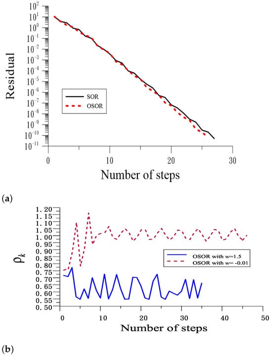
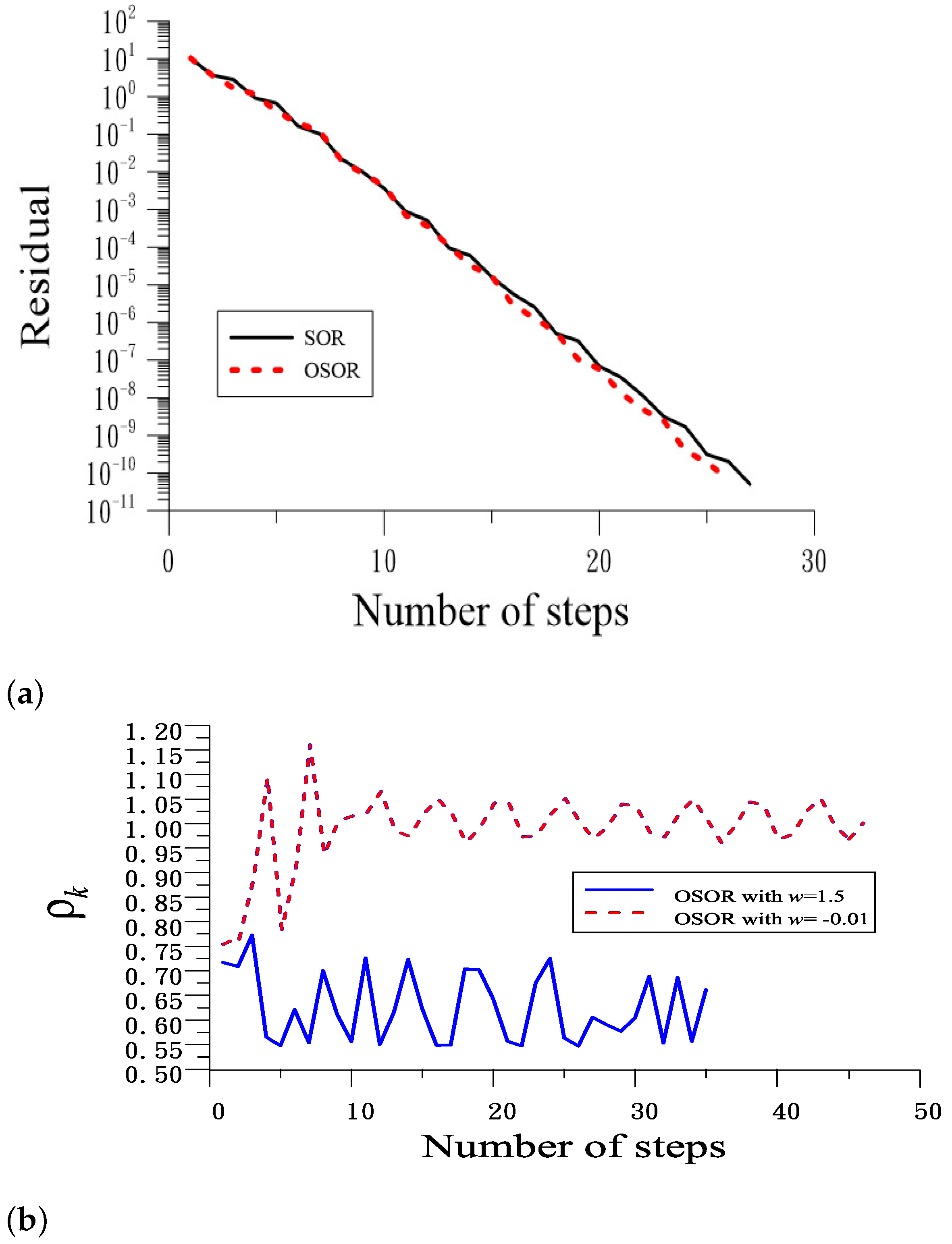
With the initial guess $x_i^0=0,i=1,\dots ,6$ and under $\epsilon ={10}^{-10}$, SOR is convergence with 27 iterations, as shown in Figure 1a. The maximum error (ME) is $1.38\times {10}^{-11}$.

Figure 1. For example 1, (a) comparing the convergence residuals obtained by SOR and OSOR, and (b) the step-by-step spectral radius of OSOR with $w=1.5$ and $w=-0.01$.

By using the OSOR with the optimal value w in Equation (85), through 26 iterations it converges, as shown in Figure 1a; ME = $2.12\times {10}^{-11}$ is obtained. In Figure 1a, the residuals obtained by SOR and OSOR with the optimal value w in Equation (85) are compared.

It is well known that, for SOR, the relaxation parameter must be $0<w<2$ for the stability of the iterative algorithm. When we take $w=1.5$, SOR is unstable, as shown in Table 1; however, as shown in Figure 1b, the spectral radius of OSOR is smaller than one at each step. Table 1 reveals that OSOR can converge with 35 steps.

Table 1. For Example 1, comparing ME and number of steps (NSs) obtained by SOR and OSOR for different values of w.

w	0.1	0.3	0.8	1.3	1.5	1.9
NS (SOR)	367	111	30	199	Divergent	Divergent
NS (OSOR)	43	39	30	30	35	47
ME (SOR)	3.91 × 10−11	3.85 × 10−11	2.22 × 10−11	2.13 × 10−11	×	×
ME (OSOR)	2.73 × 10−11	2.42 × 10−11	2.49 × 10−11	1.62 × 10−11	1.36 × 10−11	1.75 × 10−11

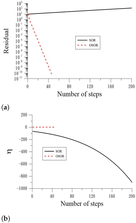
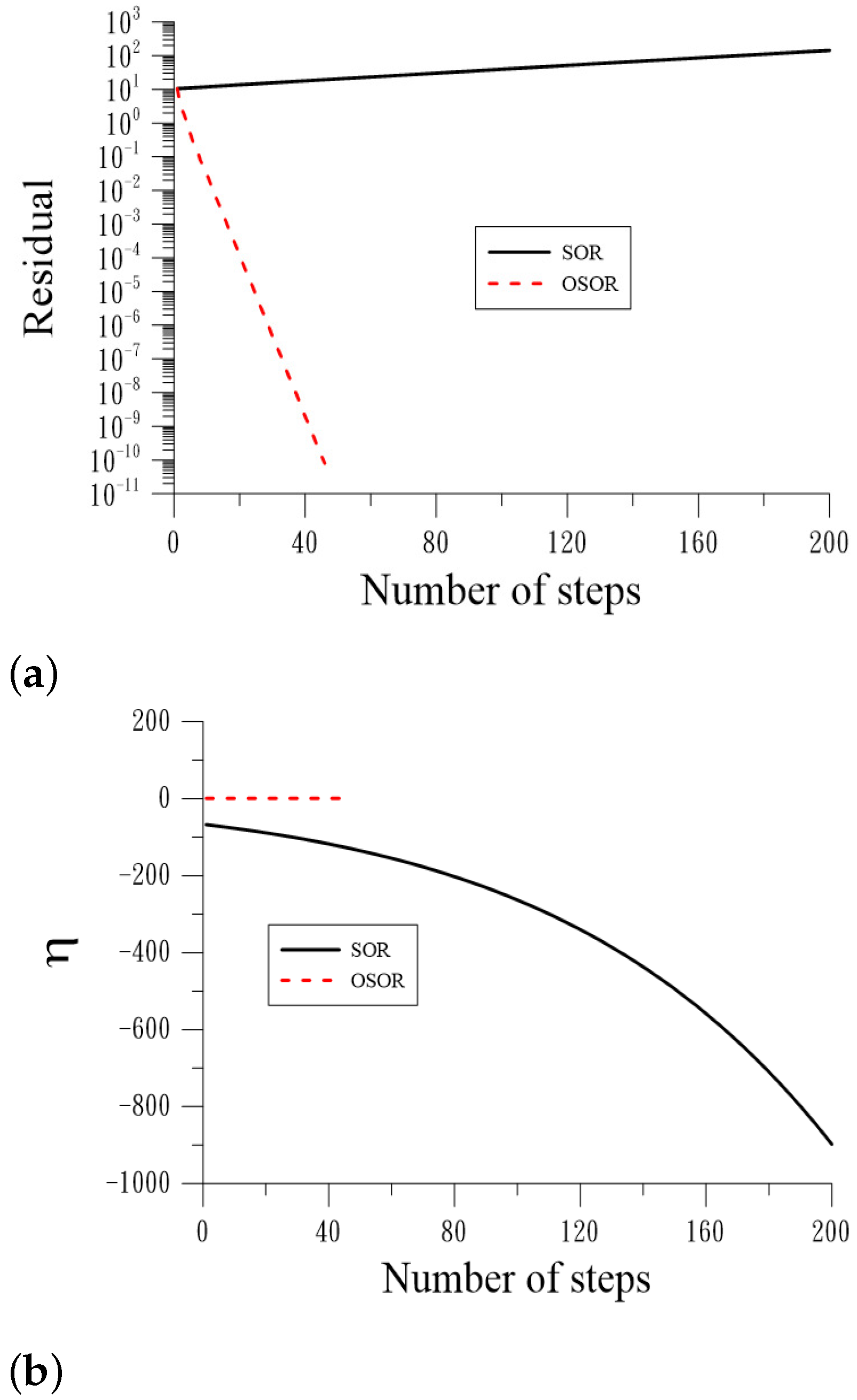
To further test the stability of SOR and OSOR, we take $w=-0.01$. In Figure 2a, we can see that SOR blows up very rapidly. Its values of ${\eta }_k$, as shown in Figure 2b, also tend to large negative values. In contrast, the OSOR method as a stabilization of SOR can seek an accurate solution with ME = $3.36\times {10}^{-11}$ within 46 steps. The values of ${\eta }_k=1$ are kept constant, as seen in Figure 2b.

Figure 2. For example 1, comparing (a) residuals and (b) $\eta$ obtained by SOR and OSOR with $w=-0.01$.

As shown in Figure 1b, the step-by-step spectral radii are oscillatory around the value of one when $w=-0.01$ is negative. The total contraction rate defined in Equation (64) is 0.6528, which is smaller than one; the OSOR iteration is convergent.

Table 1 compares ME and number of steps (NSs) obtained by SOR and OSOR for different values of w. It can be seen that SOR is sensitive to the values of w; when $w\le 0.3$, it requires more than 100 steps for the convergence, and when $w\ge 1.5$, it blows up. When $w=0.1$, we find that many ${\eta }_k$ in SOR are negative, which cause the slow convergence of SOR with 367 steps. In contrast to SOR, OSOR is very stable, not sensitive to the values of w. The OSOR method can not only stabilize SOR and also enhance the accuracy. For OSOR, w can range in a large interval $w\in (-2,2.5]$.

For SSOR, the optimal value like that in Equation (85) is not available. It is interesting that, when we use the sun-optimal value of $w=0.90169944$ in SSOR obtained from Equation (37), we can achieve a highly accurate solution within 19 steps to obtain ME = $1.50\times {10}^{-11}$.

Table 2 compares the ME and NS obtained by SSOR and OSSOR for different values of w. The improvement of NS made by OSSOR is obvious. For SSOR, the range is $w\in (0,2)$. For OSSOR, w can range in a large interval $w\in [-2.2,2.6]$.

Table 2. For Example 1, comparing ME and NS obtained by SSOR and OSSOR for different values of w.

w	0.1	0.3	0.8	1.3	1.5	1.9
NS (SSOR)	183	55	15	26	40	238
NS (OSSOR)	22	20	16	16	20	24
ME (SSOR)	3.59 × 10−11	3.03 × 10−11	1.67 × 10−11	8.29 × 10−12	8.59 × 10−12	8.59 × 10−12
ME (OSSOR)	2.74 × 10−11	1.15 × 10−11	2.57 × 10−11	1.41 × 10−11	1.02 × 10−11	1.70 × 10−11

We take $\epsilon ={10}^{-15}$. Table 3 compares NS and ME obtained by using the optimal value of $w_{opt}=1.016288735$ for SOR, and the sub-optimal values of w obtained from Equation (37) for SOR, and from Equation (67) for OSOR. $w=0.90169944$ is obtained for SOR; $w=1.00251249$ is obtained for OSOR.

Table 3. For Example 1, comparing ME and NS obtained by OSOR for optimal and sub-optimal values of w.

w	1.01628874	Equation (37)	Equation (67)
NS	39	35	37
ME	2.22 × 10−16	2.22 × 10−16	1.11 × 10−16

Table 4 extends the results in Table 3 to that for OSSOR.

Table 4. For Example 1, comparing ME and NS obtained by OSSOR for optimal and sub-optimal values of w.

w	1.01628874	Equation (37)	Equation (67)
NS	31	27	23
ME	2.22 × 10−16	2.22 × 10−16	2.22 × 10−16

As an application of Theorem 2, we can apply AOR to stabilize SOR, when SOR is unstable with $w=1.5$, as shown in Table 1.

From Equation (27), the iteration matrix for AOR is given by

$$\mathbf{G}={\mathbf{I}}_n-\sigma {(\mathbf{D}-w\mathbf{L})}^{-1}\mathbf{A}.$$

(86)

Unlike ${\mathbf{G}}_k$ for the OSOR method, the above $\mathbf{G}$ is a constant matrix.

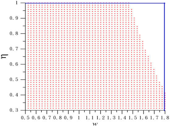
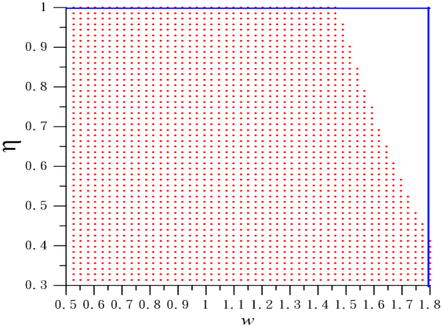
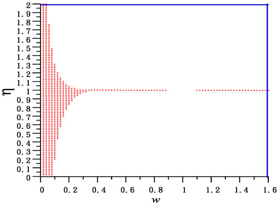
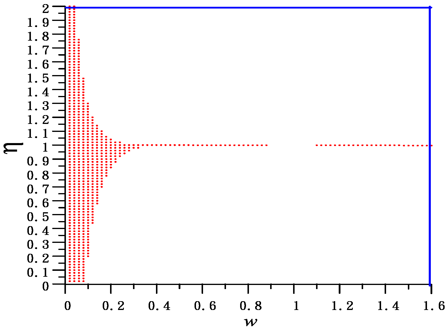
For the stability of AOR, the spectral radius $\rho \left(\mathbf{G}\right)$ must be smaller than one. We plot the stability region in Figure 3. When SOR, corresponding to $\eta =1$, is unstable with $w>1.488$, AOR can be stabilized by taking a suitable value of $\eta =\sigma /w$, such that $(w,\eta )$ locates inside the stable region.

Figure 3. For example 1, the stable region of AOR in the plane $(w,\eta )$. When $(w,\eta )$ locates inside the blank part, AOR is unstable.

In Table 5, we fix $\epsilon ={10}^{-10}$ and $w=1.5$, but with different values of $\eta =\sigma /w$ in AOR to compute the solution.

Table 5. For Example 1, comparing ME and NS obtained by the AOR with a fixed value $w=1.5$, but for different values of $\eta =\sigma /w$.

$\mathit{\eta }$	0.3	0.4	0.6	0.7
NS	66	45	43	76
ME	1.73 × 10−11	1.63 × 10−11	2.46 × 10−11	2.03 × 10−11

5.2. Example 2

We apply SOR, OSOR, and OSSOR to solve the following boundary value problem:

$$u^{″}\left(x\right)=f\left(x\right),u\left(0\right)=0,u\left(1\right)=0.$$

(87)

The exact solution is supposed to be

$$u\left(x\right)=sin\pi x.$$

(88)

The finite difference discretization of Equation (87) is

$$\begin{array}{c}\frac{1}{{\left(\mathrm{\Delta }x\right)}^2}(u_{i+1}-2u_i+u_{i-1})-f\left(x_i\right)=0,i=1,\dots ,n,\hfill \\ u_0=0,u_{n+1}=0,\hfill \end{array}$$

(89)

where $\mathrm{\Delta }x=1/(n+1)$ and $x_i=i\mathrm{\Delta }x=i/(n+1),i=1,\dots ,n$.

We take $n=99$ and $\epsilon ={10}^{-5}$. On the other hand, we have [32,34,35]

$$w_{opt}=\frac{2}{1+sin\left(\pi \mathrm{\Delta }x\right)}=1.939091659.$$

(90)

Table 6 compares the ME and NS obtained by SOR and OSOR for different values of w. It is apparent that OSOR is convergent faster than SOR when w is not the optimal value. Due to the fact that the coefficient matrix is symmetric, SSOR and SSOR are not convergent faster than SOR and OSOR.

Table 6. For Example 2, comparing ME and NS obtained by SOR and OSOR for different values of w.

w	1.5	1.6	1.7	1.8	1.9
NS (SOR)	>2000	1748	1292	855	411
NS (OSOR)	1363	1154	943	671	378
ME (SOR)	8.80 × 10−4	2.76 × 10−4	1.69 × 10−4	7.66 × 10−5	2.34 × 10−5
ME (OSOR)	5.29 × 10−4	3.44 × 10−4	2.31 × 10−4	1.57 × 10−4	2.54 × 10−5

Table 7 compares the NS and ME obtained by using the optimal value of $w_{opt}=1.939091659$ for SOR, and the sub-optimal values of $w=1.9381966$ obtained from Equation (37) for SOR, and $w=1.9381966$ from Equation (67) for OSOR.

Table 7. For Example 2, comparing ME and NS obtained by SOR and OSOR for optimal and sub-optimal values of w.

	SOR	SOR	OSOR	OSOR
w	Equation (90)	GSSA	Equation (90)	GSSA
NS	202	201	229	229
ME	9.27 × 10−5	9.25 × 10−5	9.14 × 10−5	9.04 × 10−5

5.3. Example 3

Consider an example of Equation (1) with $\mathbf{A}=\left[a_{ij}\right],a_{ij}=2i+3j,i,j=1,\dots ,n$. Suppose that $b_i=1,i=1,\dots ,n$, and exact solutions of $x_i^0$ are unknown. The initial values are $x_i^0=0,i=1,\dots ,n$.

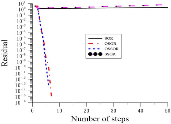
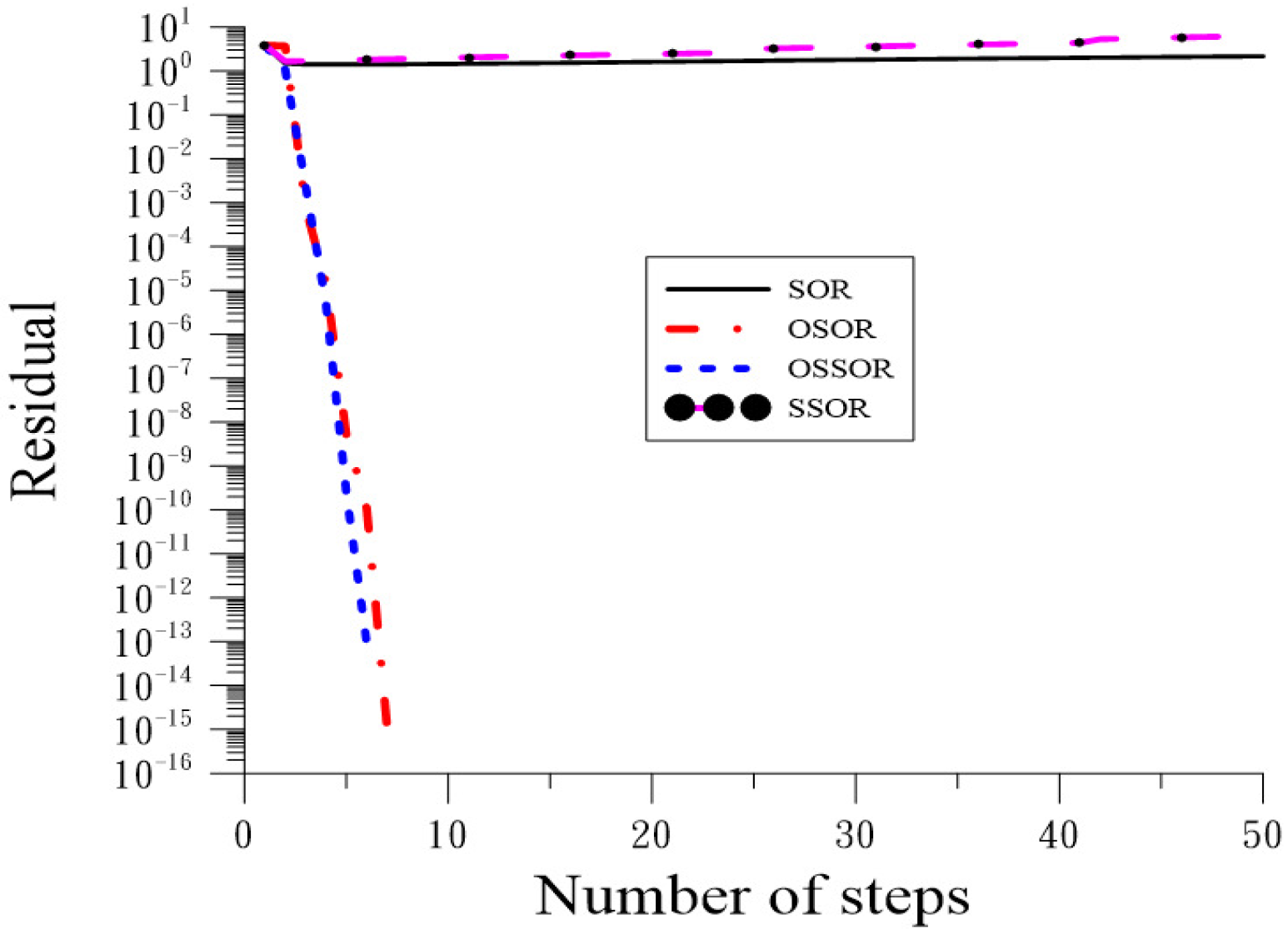
With $n=15$, under $\epsilon ={10}^{-10}$, OSOR and OSSOR using GSSA at each step are convergent with seven and six steps, respectively, as shown in Figure 4. However, both SOR and SSOR are not convergent.

Figure 4. For Example 3, comparing the convergence residuals obtained by SOR, OSOR, SSOR, and OSSOR. SOR and SSOR do not converge.

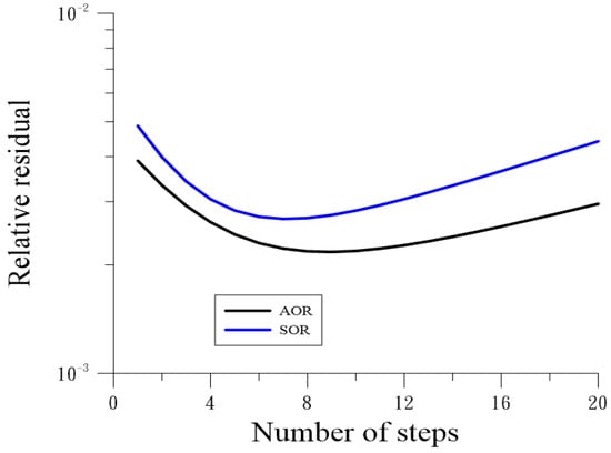
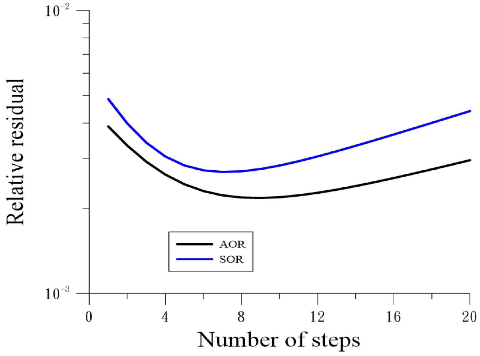
For the stability of AOR, the spectral radius $\rho \left(\mathbf{G}\right)$ must be smaller than one. We plot the stability region in Figure 5. Although we take $w=0.02$ and $\eta =1$ in the stable region in Figure 4, SOR is divergent under $\epsilon =2.8\times {10}^{-3}$. Therefore, we take the convergence criterion for the relative residual $\parallel {\mathbf{x}}_{k+1}-{\mathbf{x}}_k\parallel <2.8\times {10}^{-3}$. As shown in Figure 6, SOR is convergent with six steps, and the AOR with $w=0.02$ and $\eta =0.8$ is convergent with four steps. However, the residual errors 1.287 and 1.685 indicate that they are incorrect solutions obtained by SOR and AOR.

Figure 5. For Example 3, the stable region of AOR in the plane $(w,\eta )$. When $(w,\eta )$ locates inside the blank part, AOR is unstable.

Figure 6. For Example 3, comparing the convergence relative residuals obtained by SOR and AOR. If residual was taken, both SOR and AOR are not convergent.

If ${10}^{-3}$ is taken as the convergence criterion of the relative residuals obtained by SOR and AOR, they are divergent again, as shown in Figure 6. In contrast, as shown in Table 8, OSOR and OSSOR can compute accurate solutions very fast.

Table 8. For Example 3, comparing NS obtained by OSOR and OSSOR for different values of n.

n	10	30	50	100
OSOR	6	6	6	10
OSSOR	6	6	6	7

5.4. Example 4

We consider a linear system in Equation (1) with [28]

$$\begin{array}{c}\mathbf{A}=\left[\begin{array}{cccccccc}-4.2& 0& 1& 1& 0& 0& 1& 1\\ 1& -4.2& 0& 1& 1& 0& 0& 1\\ 1& 1& -4.2& 0& 1& 1& 0& 0\\ 0& 1& 1& -4.2& 0& 1& 1& 0\\ 0& 0& 1& 1& -4.2& 0& 1& 1\\ 1& 0& 0& 1& 1& -4.2& 0& 1\\ 1& 1& 0& 0& 1& 1& -4.2& 0\\ 0& 1& 1& 0& 0& 1& 1& -4.2\end{array}\right],\hfill \\ \mathbf{b}=\left[\begin{array}{c}-6.1\\ -5.4\\ 9.2\\ 0\\ -6.2\\ -1.2\\ 13.4\\ -4.2\end{array}\right],\mathbf{x}=\left[\begin{array}{c}1\\ 2\\ -1\\ 0\\ 1\\ 1\\ -2\\ 1\end{array}\right].\hfill \end{array}$$

(91)

By using GSSA, the sub-optimal value $w=0.9975$ for OSOR is found.

The initial values are $x_i^0=0,i=1,\dots ,8$, and under $\epsilon ={10}^{-7}$ for the relative residual, OSOR is convergent with 40 steps. In Table 9, ME and NS are compared to that obtained in [28] by using the RSORJ and RJSOR methods; they used the two-step techniques, and the optimal value $w=1.85$ is used.

Table 9. For Example 4, comparing ME and NS obtained by OSOR, OSSOR, RSORJ, and RJSOR.

	OSOR	OSSOR	RSORJ	RJSOR
ME	3.06 × 10−7	4.48 × 10−7	5.20 × 10−7	2.42 × 10−7
NS	40	22	38	38

In Table 10, the NSs obtained by OSOR and OSSOR are compared to those obtained in [36] by using the algorithms of Gauss–Seidel (GS), refinement of Gauss–Seidel (RGS), second refinement of Gauss–Seidel (SRGS), and third refinement of Gauss–Seidel (TRGS).

Table 10. For Example 4, comparing NS obtained by OSOR, OSSOR, GS, RGS, SRGS, and TRGS.

	OSOR	OSSOR	GS	RGS	SRGS	TRGS
NS	40	22	88	44	30	22

6. Conclusions

In this paper, we have re-examined the SOR method from the aspects of preserving the orthogonality of consecutive residual vector and maximizing the decreasing length of residual vector. They can significantly accelerate the convergence speed by using the OSOR method. If ${\eta }_k={\mathbf{r}}_k^T\mathbf{A}{\mathbf{u}}_k/{\parallel \mathbf{A}{\mathbf{u}}_k\parallel }^2$ in SOR was ${\eta }_k<1/2$ during the iterations, it is unstable. For the SOR method, we can improve it such that the orthogonality is preserved automatically, and simultaneously the length of the residual vector is reduced maximally. It brings the SOR method to an orthogonalized successive over-relaxation (OSOR) method. Meanwhile, the orthogonalized symmetric successive over-relaxation (OSSOR) method was developed. The OSOR and OSSOR methods preserved the orthogonality automatically and had the property of absolute convergence.

The main features of the present paper are pointed out as follows:

(a)

A new form of SOR was derived in terms of descent vector and residual vector.

(b)

We proved that the AOR method can be generated from the new form of SOR, by inserting $\eta$ preceding the descent vector in the SOR method.

(c)

The OSOR method was developed by using the extrapolated parameter $\eta$ varying step-by-step, which controlled the stability of the OSOR algorithm.

(d)

The convergence behavior of OSOR is superior than SOR; for OSOR even with a negative value of w was permitted. Hence, the stability region of OSOR was enlarged significantly.

(e)

For non-symmetric linear systems, the orthogonalized SSOR (OSSOR) method outperforms the SSOR method.

(f)

We proposed minimization techniques to choose the sub-optimal values of the relaxation parameter, which can improve the accuracy of the OSOR and OSSOR methods.

In the near future, we may examine other splitting iteration methods including two or more parameters, as well as the general $(\mathbf{M},\mathbf{N})$ splitting methods for two-block linear systems from the two aspects of preserving the orthogonality and maximally reducing the length of the residual vector by using the stabilizing factor ${\eta }_k$ in the iterative formulas.

References

- Young, D.M. Iterative methods for solving partial difference equations of elliptic type. Trans. Am. Math. Soc. 1954, 76, 92–111. [Google Scholar] [CrossRef]
- Young, D.M. Iterative Solution of Large Linear Systems; Academic Press: New York, NY, USA, 1971. [Google Scholar]
- Kincaid, D.R. Celebrating fifty years of David M. Young’s successive overrelaxation method. In Numerical Mathematics and Advanced Applications: Proceedings of ENUMATH 2003 the 5th European Conference on Numerical Mathematics and Advanced Applications, Prague, August 2003; Springer: Berlin/Heidelberg, Germany, 2004; pp. 549–558. [Google Scholar]
- Hadjidimos, A. Accelerated overrelaxation method. Math. Comput. 1978, 32, 149–157. [Google Scholar] [CrossRef]
- Albrecht, P.; Klein, M.P. Extrapolated iterative methods for linear systems. SIAM J. Numer. Anal. 1984, 21, 192–201. [Google Scholar] [CrossRef] [Scilit]
- Hadjidimos, A. Successive overrelaxation (SOR) and related methods. J. Comput. Appl. Math. 2000, 123, 177–199. [Google Scholar] [CrossRef] [Scilit]
- Bai, Z.Z.; Chi, X.B. Asymptotically optimal successive overrelaxation method for systems of linear equations. J. Comput. Math. 2003, 21, 603–612. [Google Scholar]
- Wen, R.P.; Meng, G.Y.; Wang, C.L. Quasi-Chebyshev accelerated iteration methods based on optimization for linear systems. Comput. Math. Appl. 2013, 66, 934–942. [Google Scholar] [CrossRef] [Scilit]
- Meng, G.Y. A practical asymptotical optimal SOR method. Appl. Math. Comput. 2014, 242, 707–715. [Google Scholar] [CrossRef] [Scilit]
- Miyatake, Y.; Sogabe, T.; Zhang, S.L. Adaptive SOR methods based on the Wolfe conditions. Numer. Algo. 2020, 84, 117–132. [Google Scholar] [CrossRef] [Scilit]
- Quarteroni, A.; Sacco, R.; Saleri, F. Numerical Mathematics; Springer Science: New York, NY, USA, 2000. [Google Scholar]
- Hadjidimos, A.; Yeyios, A. Symmetric accelerated overrelaxation (SAOR) method. Math. Comput. Simul. 1982, XXIV, 72–76. [Google Scholar] [CrossRef] [Scilit]
- Yeyios, A. A necessary condition for the convergence of the accelerated overrelaxation (AOR) method. J. Comput. Appl. Math. 1989, 26, 371–373. [Google Scholar] [CrossRef] [Scilit]
- Liu, C.S. A feasible approach to determine the optimal relaxation parameters in each iteration for the SOR method. J. Math. Res. 2021, 13, 1–9. [Google Scholar] [CrossRef] [Scilit]
- Liu, C.S.; El-Zahar, E.R.; Chang, C.W. Dynamical optimal values of parameters in the SSOR, AOR and SAOR testing using the Poisson linear equations. Mathematics 2023, 11, 3828. [Google Scholar] [CrossRef] [Scilit]
- Darvishi, M.T.; Hessari, P. Symmetric SOR method for augmented systems. Appl. Math. Comput. 2006, 183, 409–415. [Google Scholar] [CrossRef] [Scilit]
- Zhang, G.F.; Lu, Q.H. On generalized symmetric SOR method for augmented systems. J. Comput. Appl. Math. 2008, 219, 51–58. [Google Scholar] [CrossRef] [Scilit]
- Darvishi, M.T.; Hessari, P. A modified symmetric successive overrelaxation method for augmented systems. Comput. Math. Appl. 2011, 61, 3128–3135. [Google Scholar] [CrossRef] [Scilit]
- Chao, Z.; Zhang, N.; Lu, Y. Optimal parameters of the generalized symmetric SOR method for augmented systems. J. Comput. Appl. Math. 2014, 266, 52–60. [Google Scholar] [CrossRef] [Scilit]
- Li, C.L.; Ma, C.F. An accelerated symmetric SOR-like method for augmented systems. Appl. Math. Comput. 2019, 341, 408–417. [Google Scholar] [CrossRef] [Scilit]
- Li, Y.; Dai, P. Generalized AOR methods for linear complementarity problem. Appl. Math. Comput. 2007, 188, 7–18. [Google Scholar] [CrossRef] [Scilit]
- Huang, Z.G.; Xu, Z.; Lu, Q.; Cui, J.J. Some new preconditioned generalized AOR methods for generalized least-squares problems. Appl. Math. Comput. 2015, 269, 87–104. [Google Scholar] [CrossRef] [Scilit]
- Zhang, C.H.; Wang, X.; Tang, X.B. Generalized AOR method for solving a class of generalized saddle point problems. J. Comput. Appl. Math. 2019, 350, 69–79. [Google Scholar] [CrossRef] [Scilit]
- Darvishi, M.T.; Khosro-Aghdam, R. Symmetric successive overrelaxation methods for rank deficient linear systems. Appl. Math. Comput. 2006, 173, 404–420. [Google Scholar] [CrossRef] [Scilit]
- Darvishi, M.T.; Khani, F.; Hamedi-Nezhad, S.; Zheng, B. Symmetric block-SOR methods for rank-deficient least squares problems. J. Comput. Appl. Math. 2008, 215, 14–27. [Google Scholar] [CrossRef] [Scilit]
- Bai, Z.Z.; Parlett, B.N.; Wang, Z.Q. On generalized successive overrelaxation methods for augmented linear systems. Numer. Math. 2005, 102, 1–38. [Google Scholar] [CrossRef] [Scilit]
- Laskar, A.H.; Behera, S. Refinement of iterative methods for the solution of system of linear equations Ax=b. IOSR J. Math. 2014, 10, 70–73. [Google Scholar] [CrossRef] [Scilit]
- Meligy, S.A.; Youssef, I.K. Relaxation parameters and composite refinement techniques. Results Appl. Math. 2022, 15, 100282. [Google Scholar] [CrossRef] [Scilit]
- Hadjidimos, A.; Yeyios, A. The principle of extrapolation in connection with the accelerated overrelaxation method. Linear Alg. Appl. 1980, 30, 115–128. [Google Scholar] [CrossRef] [Scilit]
- Missirlis, N.M.; Evans, D.J. The extrapolated successive overrelaxation (ESOR) method for consistently ordered matrices. Int. J. Math. Math. Sci. 1984, 7, 361–370. [Google Scholar] [CrossRef] [Scilit]
- Milewski, S.; Orkisz, J. In search of optimal acceleration approach to iterative solution methods of simultaneous algebraic equations. Comput. Math. Appl. 2014, 68, 101–117. [Google Scholar] [CrossRef] [Scilit]
- Yang, S.; Gobbert, M.K. The optimal relaxation parameter for the SOR method applied to the Poisson equation in any space dimensions. Appl. Math. Lett. 2009, 22, 325–331. [Google Scholar] [CrossRef] [Scilit]
- Golub, G.H.; Van Loan, C.F. Matrix Computations; The Johns Hopkins University Press: Baltimore, MA, USA, 1996. [Google Scholar]
- Watkins, D.S. Fundamentals of Matrix Computations, 2nd ed.; Wiley: New York, NY, USA, 2002. [Google Scholar]
- Demmel, J.W. Applied Numerical Linear Algebra; SIAM: Philadelphia, PA, USA, 1997. [Google Scholar]
- Audu, K.J.; Essien, J.N. An accelerated iterative technique: Third refinement of Gauss-Seidel algorithm for linear systems. Comput. Sci. Math. Forum 2023, 7, 7. [Google Scholar] [CrossRef] [Scilit]
Disclaimer/Publisher’s Note: The statements, opinions and data contained in all publications are solely those of the individual author(s) and contributor(s) and not of MDPI and/or the editor(s). MDPI and/or the editor(s) disclaim responsibility for any injury to people or property resulting from any ideas, methods, instructions or products referred to in the content. |
© 2024 by the authors. Licensee MDPI, Basel, Switzerland. This article is an open access article distributed under the terms and conditions of the Creative Commons Attribution (CC BY) license (https://creativecommons.org/licenses/by/4.0/).