1. Introduction
The discrete choice model (DCM) has rapidly become popular due to its practical applicability and theoretical robustness under individual preferences. The primary interest in the DCM was in the context of transportation. The contribution of [
1] played a vital role from the 1970s to 1990. Since that time, the DCM has only been considered a realistic behavior of choice model when used as a closed-form model like nested logit, an open-form model like mixed logit, and a latent class model.
The satisfaction of occupants in office buildings is linked to various factors, including the indoor environmental quality (such as thermal, visual, and air quality and acoustic conditions), as well as the characteristics of the workspace and the building itself, such as the size, esthetics, furniture, and cleanliness. The ten studies listed in
Table 1 have acknowledged the parameters that constitute occupants’ satisfaction with buildings (see, e.g., [
2,
3,
4,
5,
6,
7,
8,
9,
10,
11,
12,
13,
14,
15,
16]).
The studies did not provide a consistent definition of occupant satisfaction. However, all of them approached occupant satisfaction broadly, linking it to either their satisfaction and well-being with the indoor environmental quality or their fulfillment and comfort with their workspace. Specifically, some studies [
2,
5,
6,
10] concentrated solely on how the indoor environmental quality influenced the satisfaction of building occupants.
Their findings indicated that the thermal, visual, and acoustic atmosphere and superior air quality influenced the building occupants’ sense of fulfillment. While the significance of various indoor environmental factors in building occupants’ satisfaction showed slight variations across studies, the thermal environment was consistently ranked as slightly more important than the air quality and the acoustic environment, and significantly more important than the visual environment.
A literature review conducted by [
17] highlighted that various non-environmental factors significantly influence building occupants’ satisfaction alongside indoor environmental factors. Factors such as occupants’ control over the indoor environment, view satisfaction, privacy levels, and office layout have been identified as crucial determinants ([
3,
4,
8,
18]). Moreover, recent advancements propose the application of machine learning techniques to enhance the examination of medical data, potentially surpassing traditional methods [
19]. The complexity of human decision making has recently highlighted the need to comprehend risky options. One study, for example, used the choices 13k dataset to train neural networks in a unique way that revealed information about decision noise and dataset bias [
20]. For various other applications, one should refer to ([
16,
21,
22,
23,
24,
25,
26]). Further, [
27] promote the development of the agent decision model and provide a new way to solve complex decision problems.
This research aims to present a latent class choice model with participant environmental feedback data in an authentic setting. In order to overcome several issues with the conventional approaches, we developed a novel hybrid latent class choice model in this study that combines a Gaussian negative binomial mixture model [
28]. To evaluate the performance of the suggested model with more conventional models, we employed micro-ecological momentary assessments (EMA) as secondary feedback data in this investigation.
Micro-EMA is a technique that utilizes a smartwatch interface to elicit and gather immediate, in-the-moment subjective feedback from an individual over several weeks [
16]. We gained insight into that person’s comfort preference patterns by obtaining an extensive volume of feedback from a single individual in various environments and comfort conditions. It is suggested that these behavioral patterns can be employed to categorize individuals into clusters based on their environmental perceptions. Consequently, grouping individuals with comparable comfort preferences could enhance the precision of forecasting where a person will feel comfortable and how the system can respond without extra sensors. Moreover, accumulating substantial quantities of subjective preference data from numerous individuals in a specific area can help define the comfort-related characteristics of that space to complement the data obtained from the installed sensors.
If it is theoretically feasible and minimally disruptive to the occupants, incorporating humans as sensors within buildings can revolutionize post-occupancy evaluations and building and system design, as well as controls and automation procedures. This opens up opportunities for individuals to contribute feedback in various scenarios, whether for short-term episodic purposes (spanning days or weeks), building commissioning extending to long-term assessments (over months or years), or continuous system control and management. This research aligns with the growing interest in other fields that leverage human input as sensors, such as event detection using cybersecurity [
18], social media data [
24], ecological momentary assessment [
29] and emergency detection [
30].
In the context of environmental measurements, previous efforts have involved the use of specific sensors mounted on mobile carts [
31,
32]. However, these sensors were not cost-effective for many building operation scenarios and the affordability issue led to the development of low-cost continuous-sensing sensors, albeit with the requirement for frequent calibration [
1,
33,
34]. Nonetheless, the placement of these sensors within buildings and the interpretation of their readings remained challenging in the literature, primarily due to the heterogeneous nature of indoor spaces [
34]. Conversely, surveys introduced their own set of challenges, such as determining the appropriate questions to ask, selecting the right respondents, and interpreting the survey results [
1]. Furthermore, [
35] explored the concept of ‘survey fatigue’, wherein survey participants become overwhelmed by the volume of questions, potentially resulting in misrepresentations in responses and decreased response rates.
The literature on choice modeling in the context of environmental perspectives is estimated to have exceeded 14,200 publications. Some of the articles related to occupant preferences and satisfaction with their findings are listed below.
The attention to discrete choice models as a hypothetically sound and practical tool for investigating choice behavior, particularly behavioral outcomes like willingness to pay, has grown rapidly. This development initially took place in the context of transportation, which was where McFadden made his initial contributions. The authors of [
1] offer a historical indication of these contributions from the 1970s to the early 1990s. Since then, there has been a significant expansion of research in the various aspects of choice modeling. This includes the development of more behaviorally realistic discrete choice model forms, such as closed-form models like nested logit, and open-form models like mixed logit, latent class, and generalized mixed logit. New data paradigms have also emerged, including mixed data approaches and expressed preference and choice studies. Additionally, process heuristics have been incorporated by researchers into choice models, such as hybrid logit models, to handle attribute endogeneity and account for attribute non-attendance [
36].
2. Model Framework
The subject model, namely the Gaussian negative binomial mixture with a latent class choice model, is presented in this section. Then, we give an extensive comparison with benchmark models, i.e., mixed logit, Multinomial Logit, and latent class choice models. We observe that our subject model efficiently performs better than the benchmark models. By including negative binomial distribution, the subject model effectively addresses overdispersion. Additionally, the presence of a latent class choice model makes it more reliable for decision making under heterogeneity. The subject model performed better under the circumstances of heterogeneity in classes and data variability.
2.1. Latent Class Choice Model
LCCM contains two models: a class membership model and a class-specific choice model. The class membership model is defined as a function of the features of decision-makers associated with a particular class. The utility
of a decision-maker ‘
m’ associated with class ‘
l’ is stated as follows:
where
is a vector of the features of decision-makers ‘
m’ and
is the corresponding vector of unknown parameters.
is an error term that follows Extreme Value Type-I distribution over decision-makers and classes, which is assumed to be i.i.d.
The probability of decision-makers ‘
m’ associated with class
‘l’ is specified decision-makers as follows:
The second model, namely, the class-specific model, is defined as the probability of selecting a particular option as a function of the observed exogenous feature option, conditioned on the person associated with class ‘
l’. The utility of an individual ‘
m’ selecting an option ‘
k’ at a time
is expressed as follows:
where
is a vector of the observed features of selecting an option ‘
k’ at the time
,
is the corresponding unknown parameter’s vector, and
is an error term that follows Extreme Value Type-I distribution. At the same time, it is assumed to be i.i.d.; the conditional probability of decision-makers ‘
m’ selecting an option ‘
k’ at a time
is given as follows:
where
K is the number of available options.
Let
be a matrix of all the individual options at time
, consisting of
order and
be
order matrix, where
The conditional probability of observing
associated with class ‘
l’ is expressed as follows:
The likelihood of an individual ‘m’ selecting an option ‘k’ can be defined by combining the conditional option probability with the probability of an individual associated with class ‘l’ as follows:
The resulting likelihood of all the decision-makers ‘
m’ can be obtained as follows:
2.2. Proposed Model
The proposed model can be obtained by replacing the class membership probability with the Gaussian negative binomial mixture model. The subject model is a hybrid machine learning approach, as it combines the advantages of two types of models (i.e., discrete and continuous) into one. For this purpose, GMM and NBMM are used for continuous and discrete variables. The vector, consisting of ‘m’ decision-makers attributes, is split into two sub-vectors, i.e., and . These two sub-vectors contain the dimensions and which equals the number of elements in and (continuous or discrete attributes) respectively.
Gaussian Negative Binomial Mixture Model
GMM is a collection of ‘L’ Gaussian densities, where each density is a segment of the mixture and has its mean and covariance matrix. The overall likelihood that it represents the mixing coefficient comes from the component ‘l’.
A useful and reliable distribution to incorporate count data is the negative binomial distribution. It is a versatile statistical tool that has gained popular significance for dealing with count data with overdispersion. The presence of multiple latent classes within the data allows the model to assume observation counts that are generated from a mixture of negative binomial models. This model can effectively capture the heterogeneity and excess variation within the data through the parameter estimation of the negative binomial mixture model and mixing proportion.
Marginal and posterior probability is estimated using Bayes’ theorem after estimating subject model probability assuming Gaussian and negative binomial distributions are independent on continuous and discrete datasets, after considering the conditional independence properties on the graphical structure of the proposed model. The joint probability can be formulated by taking the product of four terms. The first term is class/label probability, and the second and third are the conditional probabilities of
and
. The fourth term contains the choice probability conditional on the class. We can represent the joint probability as follows:
where
where
vectors of favorable features and
is the discrete characteristics of decision-makers ‘
m’,
is the number of
and
which are the corresponding mean vectors of continuous and discrete distributions.
2.3. Joint Probability
The joint probability of
,
, and
can be accessed by using Equation (8)’s overall component ‘
k’:
where
and
are matrices containing the ‘
L’ mean vectors of continuous and discrete variables,
is a matrix containing ‘
L’ covariance matrices
, and
is a matrix containing the
L vectors of
. By omitting the dependencies on the left-hand side of the equation to make the notation more assembled,
The overall joint probability can be estimated by using different methods (i.e., maximum likelihood estimation, Hessian Matrix, and Expectation Maximization Algorithm). The traditional maximum likelihood estimation method is inscrutable due to the summation over ‘
L’ that will appear inside the equation on both LCCM and GNBM-LCCM. However, as the number of parameters increases in the model, the MLE becomes more burdensome and lengthened. In addition, the empirical singularity problems might arise during the Hessian Matrix procedures and become numerically challenging, [
37]. Therefore, the EM algorithm is an effective way to overcome all these problems. Moreover, it is a powerful technique to estimate the parameters with latent variables.
2.4. EM Algorithm
The EM algorithm is divided into two steps, expectation and maximization steps, respectively, as follows:
E-step: This step starts first by taking the joint likelihood function as follows:
Then, taking the logarithm of the likelihood, the probability breaks the function into two separate terms, i.e., the class membership model and the class-specific choice model.
Now, we find the value of
by taking the expectation using the Bayes theorem.
It is important to note that in Equation (9) and in Equation (16) contemplate prior probability and corresponding posterior probabilities, respectively.
M-step: In this step, the unknown parameters are estimated, since, in the presence of latent variable
, Equation (16) cannot be estimated directly. Making use of Equations (16) and (19), it gives the following:
By taking the derivatives of unknown parameters and setting them to zero, we obtained the following:
where
Overall, the EM algorithm revolves between E-step and M-step until convergence is attained. First, the unknown parameters are estimated. Second, the latent variable (Equation (19)) is estimated by taking the expectation using the Bayes Theorem. In addition, the closed-form solution of the parameters is derived (from Equation (21) to Equation (24)). Finally, the log-likelihood is examined by utilizing the obtained values of the unknown parameters and then scrutinized for convergence. If the convergence benchmark is not reached, we return to E-step. From Equation (21) to Equation (24), the closed-form solution is available for maximizing coefficient, the Gaussian mean matrix, the negative binomial mean matrix, and Gaussian covariance matrix, respectively. Regarding Equation (25), we cannot obtain any closed-form solution for the parameter . For this purpose, the Gradient-Based Numerical Optimization method is used.
2.5. Final Likelihood
After attaining convergence, the marginal probability of observing a vector of ‘
t’ options of all the decision-makers ‘
M’ is examined as follows:
where
is the posterior probability of the vector
being obtained by the cluster ‘
l’.
The posterior probability can be expressed using Bayes theorem as follows:
The above posterior probability of Equation (27) can be used to compare the GNBM-LCCM and traditional LCCM from Equation (7). Further, it is used to compute extrapolated sample prediction accuracy.
2.6. Real-Life Application with Discussion
Dataset Overview: This dataset comprises data collected from the BUDS lab deployments of the Cozie Fitbit smartwatch platform. It involves collecting intensive longitudinal subjective feedback regarding comfort-based preferences through micro-ecological momentary assessments on a smartwatch platform. In an experiment conducted over two weeks with 30 occupants, a total of 4378 field-based surveys were generated to assess thermal, noise, and acoustic preferences.
Throughout the entire study, the environmental variables (such as temperature and relative humidity) in three different buildings were observed. The participants used an open-source application called Cozie on their smartwatches to complete comfort surveys. Additionally, a custom-designed smartphone application constantly tracked their indoor locations. This location data allowed us to accurately synchronize the timing and spatial aspects of environmental measurements with the thermal preference responses provided by the participants.
In order to extract valuable insights from the dataset, we initiated the exploration by carefully reviewing the features and their corresponding descriptions (refer to
Table 2). This preliminary examination served as an informative starting point, granting us a holistic understanding of the dataset’s contents. It facilitated the identification of essential variables that play a pivotal role in shaping user choice behavior. These key variables were subsequently selected for more in-depth analysis and model development.
Table 3 presents the mean matrix illustrating the class membership model of the subject data. This matrix offers valuable insights into the distribution of the occupants among the different latent classes within the dataset. Through an examination of this mean matrix, we can gain an understanding of the likelihood of users belonging to each class and identify the underlying class structure within our hybrid model.
Figure 1 graphically represents the majority of the data attributes in the case where the distribution of Environmental Light values already exhibits a noticeable overlap for various visual feedback (located at the top-middle distribution in
Figure 2).
The variable ‘time’ was generated by employing feature engineering techniques on the timestamps corresponding to when the occupants provided feedback. This engineered feature represents the time cyclically, taking into account both the hour of the day and the day of the week. This straightforward feature type was integrated into all the scenarios to identify potential cyclical patterns or factors influencing preference prediction. The attribute ‘time’ is used to categorize the class membership model into distinct classes, as follows: Class L = 1: This initial latent class corresponds to environmental data recorded from September 28th to October 10th. These applications represent a specific group characterized by an early time frame. Class L = 2: The second class is associated with applications recorded from October 11th to October 22nd. Class L = 3: The third class is related to periods spanning from October 23rd to November 3rd. Class L = 4: The fourth and final class comprises applications with a time frame from November 4th to November 15th, representing the last observation period for the occupants. These class assignments help delineate the temporal structure of the dataset and provide a meaningful segmentation of the occupant observations. This finding strengthens the argument that relying solely on environmental measurements is insufficient for characterizing an individual’s preferences, thus leading to less accurate predictions, as has been observed in earlier research [
7].
Table 4 provides an overview of the parameter estimation in the class-specific choice model. This table offers insights into the estimated parameters for each latent class within the hybrid model. These estimated parameters enable us to quantitatively assess the influence of different variables on the choice behavior of users within each class. The proposed model facilitated the division and categorization of these zones, now based on the various comfort praeferences exhibited by the occupants in those areas. This outcome primarily offered facility managers an overview of the office spaces they oversee, equipping them with insights to enhance comfort and take necessary actions.
In
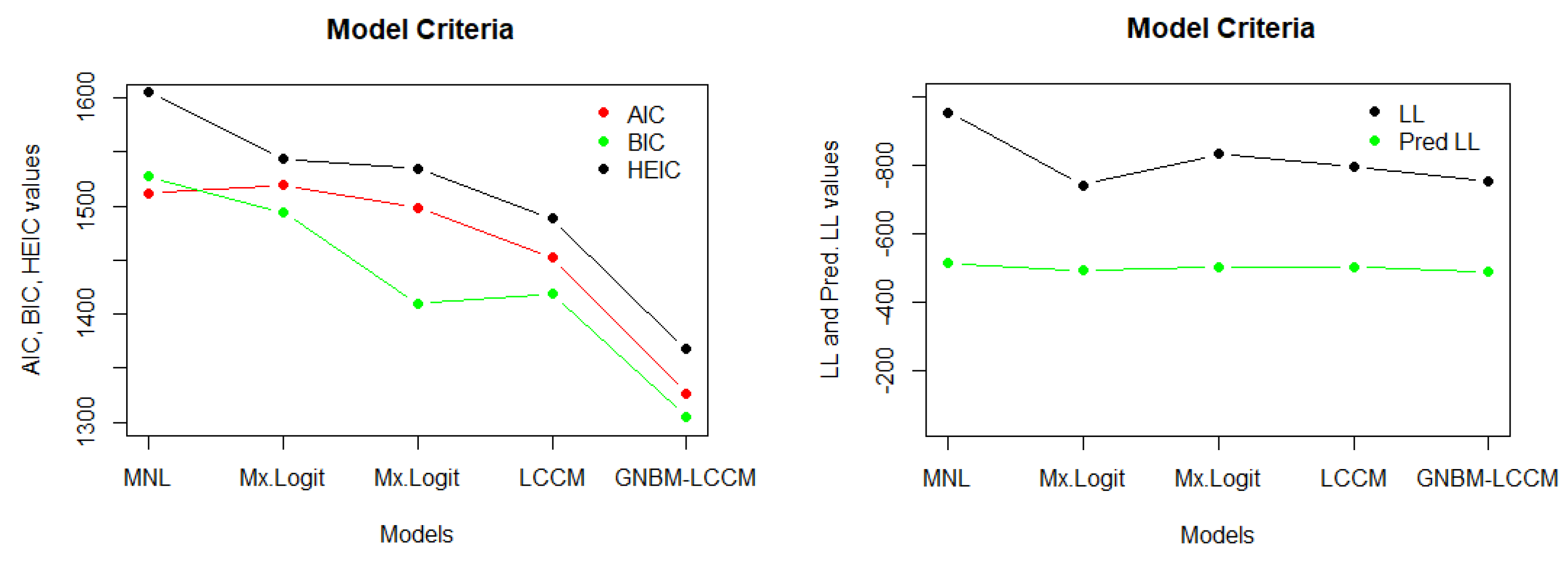
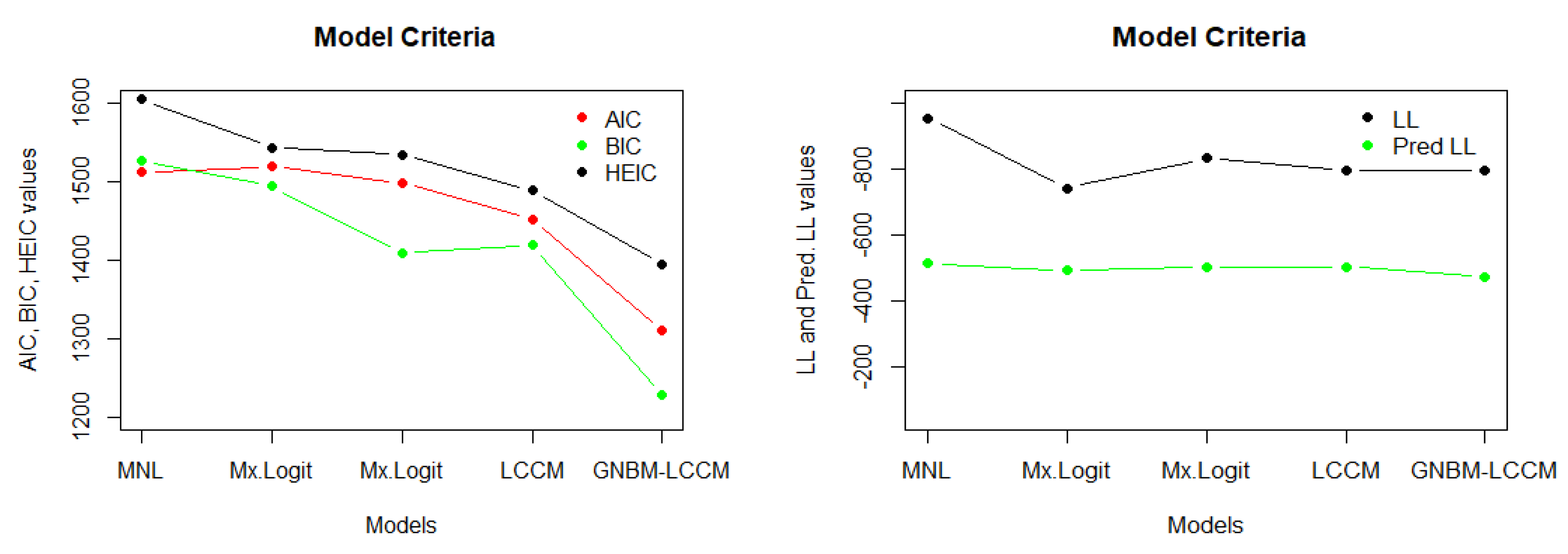
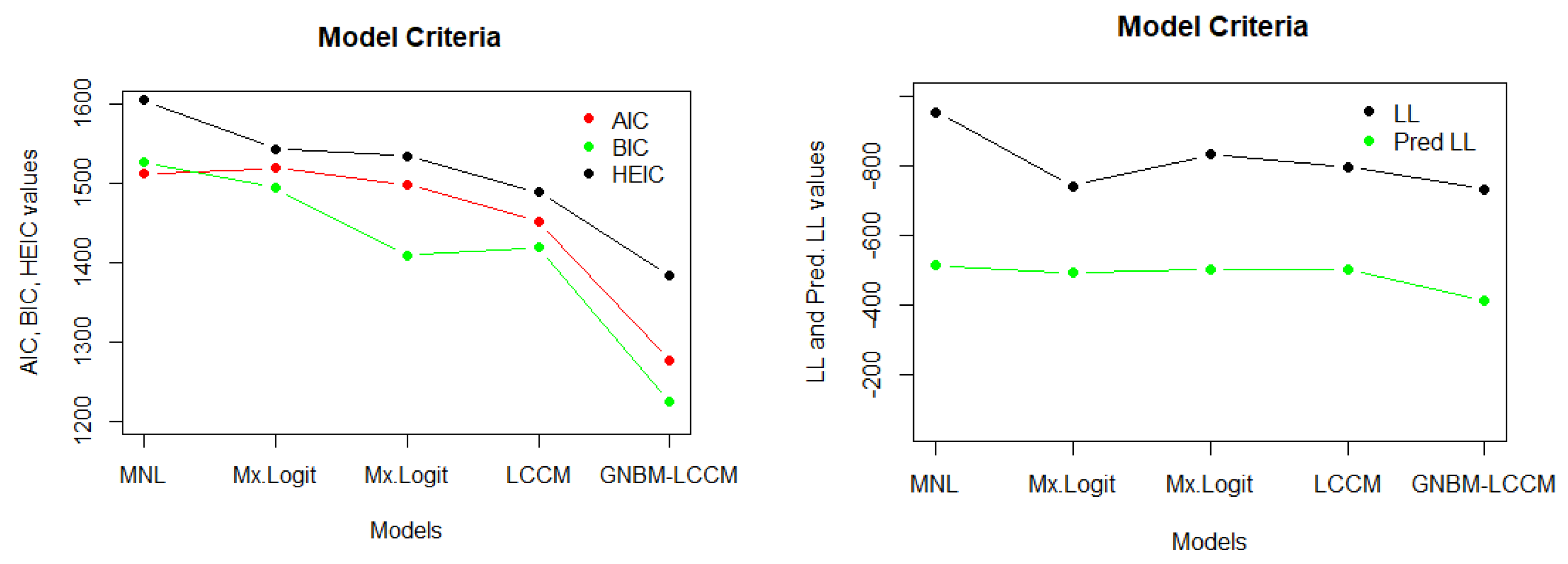
Table 5, we compare the proposed Gaussian negative binomial mixture with a latent class choice model (GNBM-LCCM) and traditional models. Our evaluation involves the use of various metrics, including AIC (Akaike Information Criterion), BIC (Bayesian Information Criterion), HEIC (Hannan–Quinn Information Criterion), LL (log-likelihood), Joint LL (Joint Log-Likelihood), and Pred LL (Predictive Log-Likelihood). This comparative assessment allows us to determine the superiority of our GNBM-LCCM over traditional models in terms of model fit, complexity, and predictive accuracy. The visual representations of these benchmark comparisons are also provided in
Figure 3,
Figure 4 and
Figure 5.
Considering the preference feedback in this methodology occurred at a notably higher frequency compared to typical surveys or occupants’ interactions with thermostats, this study possessed preference data characterized by a relatively diverse temporal and spatial nature. In the initial observation, it is apparent that the office space generally provided a comfortable environment, whereas outdoor seating areas exhibited an overall higher preference for cooling. The study also captured time-dependent fluctuations, revealing the model’s capability to predict comfort preferences that varied across different times of the day or days of the week. Notably, within the office environment, there was a peak in warmer preference around mid-day. However, it is worth noting that the model sometimes attempted to predict comfort preferences inaccurately during periods when no data were available. The square peaks observed in the office area for aural and visual prediction, particularly between the hours of 22:00 and 7:00, were a result of the absence of data to make accurate predictions during those times.
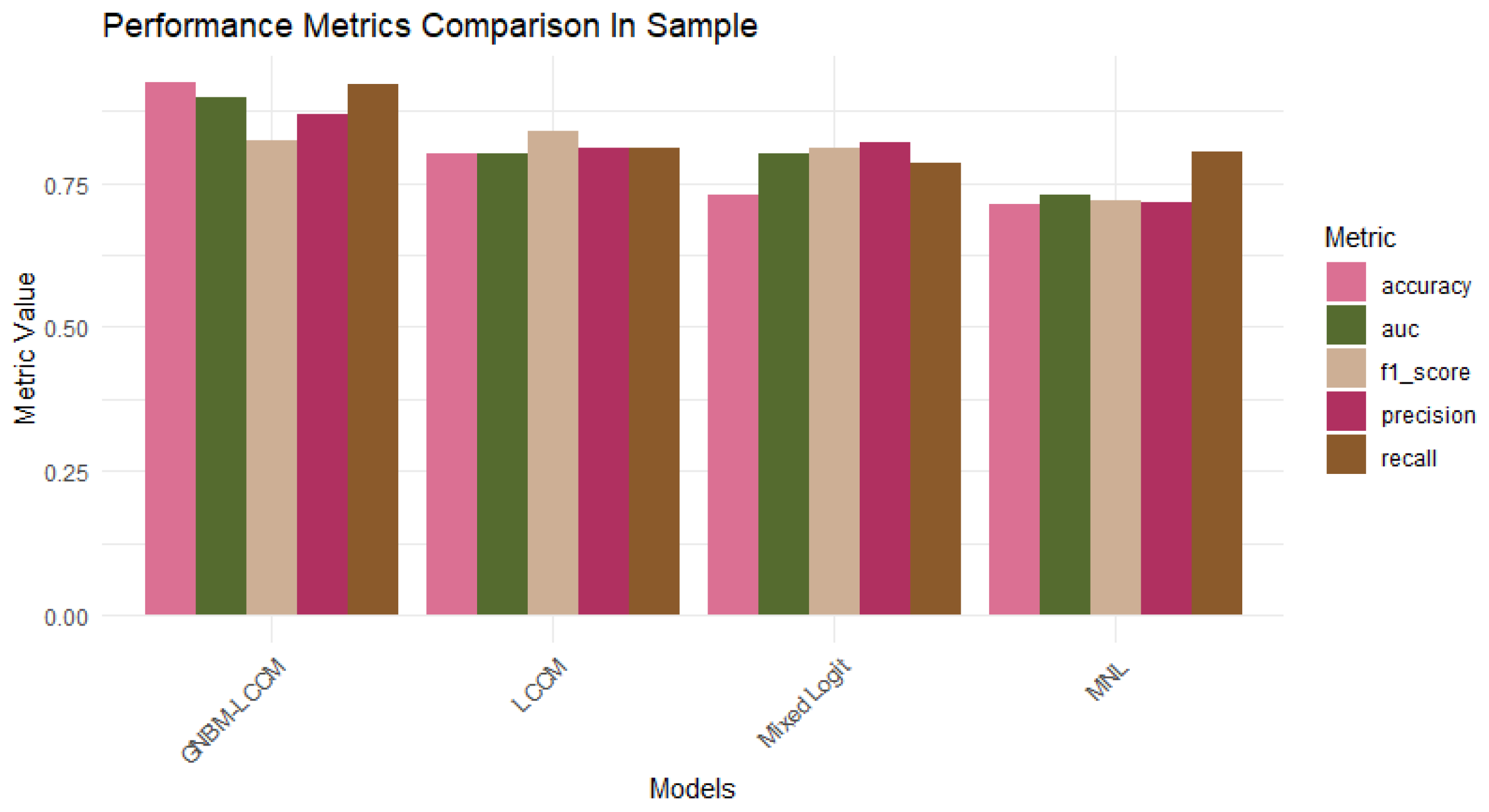
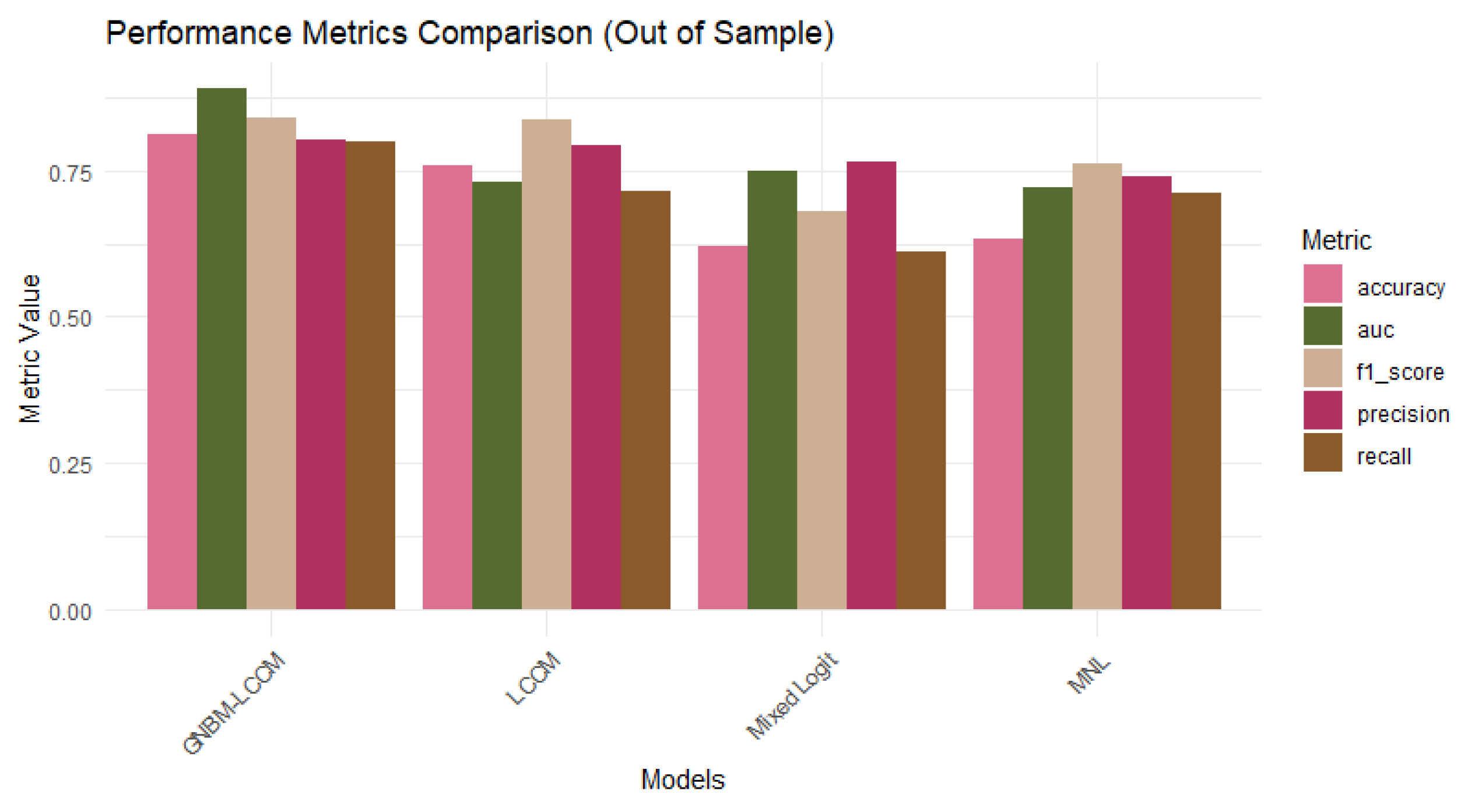
Figure 6 and
Figure 7 provide a comprehensive comparison of the performance metrics for four models: MNL, mixed logit, LCCM, and GNBM-LCCM, evaluated both in-sample and out-of-sample.
Table 6 illustrates the in-sample evaluation criteria, where the GNBM-LCCM consistently outperforms the benchmark models across most metrics. Specifically, the GNBM-LCCM demonstrates superior accuracy (0.9246), Recall (0.9204), precision (0.8693), and AUC (0.8971), with only a slight dip in the F1 Score (0.8249) compared to LCCM (0.8396). These results indicate that the GNBM-LCCM not only enhances the predictive accuracy but also effectively captures the intricacies of decision-making processes within the sample data.
Table 7 extends this evaluation to out-of-sample performance, where the GNBM-LCCM maintains its dominance over the traditional models. The GNBM-LCCM achieves the highest accuracy (0.8103), AUC (0.8901), competitive Recall (0.7983), F1 Score (0.8398), and precision (0.8024). These metrics suggest that the GNBM-LCCM is robust and generalizes well to unseen data, thus providing reliable predictions beyond the training dataset. In contrast, the mixed logit model shows the weakest performance out-of-sample, with lower accuracy (0.6197) and Recall (0.6115), highlighting its limitations in generalizability. The reliable performance of both the in-sample and out-sample evaluation criteria of the subject model makes it a more robust and accurate choice model.
3. Conclusions
In this study, an innovative hybrid choice model has been introduced, namely the Gaussian negative binomial mixture with latent class choice model (GNBM-LCCM). Further, we have checked its practical application by implementing this to environmental preference data. Our primary objective was to make it more reliable as compared to benchmark studies, i.e., Multinomial Logit model, mixed logit model, and latent class choice model (LCCM). By this comparison, we have proved the superior performance of our subject model. The results demonstrate that the proposed model not only outperforms in-sample evaluation, but it also shows superior performance for out-of-sample criteria.
All of the previous studies effectively represent the heterogeneity in individual preferences, but they fail to deal with the overdispersion situation. The benchmark models such as the Multinomial Logit and latent class choice models could easily depict the decision-making process, but it is not accurate in complex criteria like the subject model. We fill the gap of the restricted comprehension of individual preferences and latent classes with overdispersion data by incorporating the hybrid model.
The decision-making process is being scrutinized by implementing GNBM-LCCM in the analysis of environmental preference data. These data are more extensively examined through GNBM with the presence of latent classes in it. These results highlight how important it is to take latent classes into account and correct for overdispersion in a choice model that not only increases its accuracy but also plays a vital role in capturing heterogeneity in individual preferences.
The subject model is a robust framework for analyzing the decision-making process; however, it faces some limitations. For example, it may give over-generalized results as the latent class follows an independent assumption. Secondly, the model performance might oversimplify the input data, especially with sparse or noisy datasets. Additionally, in large-scale applications, parameter estimation may lead to false predictions, which require more consideration of computational complexity.
Therefore, future research could focus on the GNBM-LCCM for large dataset scalability and model performance. The applicability and robustness of the subject model could investigate different areas using different datasets. Finally, the advancement of the subject model could be enhanced by adding an alternative regularization technique with sparse or noisy data.


 and
and 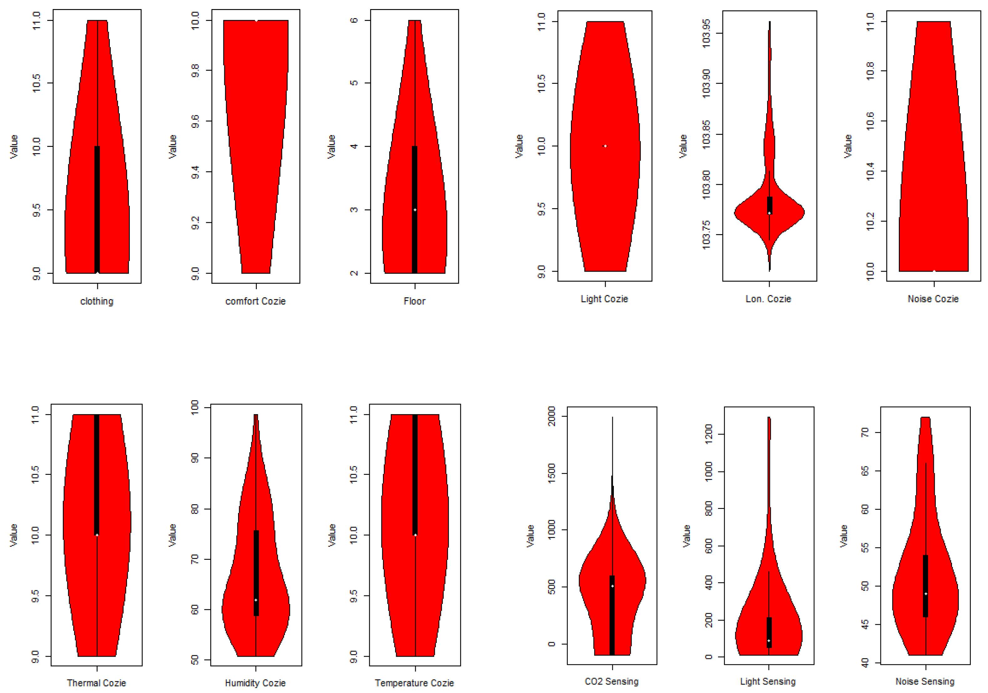

