An Improved Simulated Annealing Sampling Method for Land-Cover Accuracy Assessment

Abstract

Landscape heterogeneity is the core attribute of land cover landscape patterns, and a critical factor that must be considered in land cover accuracy assessment. This paper regards sampling in land cover accuracy assessment as essentially a multi-objective optimization problem, where uniform distribution avoids spatial autocorrelation while accounting for landscape heterogeneity to enhance the robustness of evaluation results. This paper proposes a land cover accuracy assessment method based on landscape index-improved simulated annealing sampling. By adopting a perturbation function that considers spatial equilibrium, it uses the Aggregation Index (AI) and Landscape Shape Index (LSI) to modify the objective function, optimizing the sample uniformity in low-heterogeneity areas and increasing the sample coverage in high-heterogeneity regions to achieve dual sampling optimization. Taking Jiangxi Province as the study area, the performance of the proposed method is verified through two experiments. In the first experiment, accuracy assessment is carried out on three sets of 30 m land cover products, namely GlobeLand30, CLCD and GLC_FCS. The two sample sets generated by LSI optimization and AI optimization yield highly consistent results in terms of User’s Accuracy (UA), Producer’s Accuracy (PA), area-weighted overall accuracy and Kappa coefficient, which demonstrates that the proposed method has stable cross-product generality. The second comparative experiment with four types of traditional sampling methods shows that the traditional methods cannot complete the accuracy assessment of three rare land categories including wetland, shrubland and bare land, and supplementary samples are required through secondary sampling. The optimized method can complete the PA and UA assessment of all land categories in a single run, while ensuring that the global overall accuracy and Kappa coefficient are consistent with those of traditional methods.

1. Introduction

Land-cover data and changes in land cover are fundamental inputs for research on food security, greenhouse gas emissions, ecosystem structure and function, water cycling and redistribution, and biogeochemical cycles [1,2,3]. The process of remote-sensing mapping of land cover involves extracting thematic attributes and spatial distributions by integrating the rich spectral and textural information, as well as spatiotemporal relationships found in airborne and satellite imagery, with ancillary data and domain knowledge. This is accomplished using methods such as mathematical statistics and interactive interpretation [4]. Owing to limitations in production techniques, land-cover datasets contain commission and omission errors, which can directly affect their effectiveness in downstream applications [5,6,7,8]. Consequently, accuracy assessment is an essential component of land-cover data production and has emerged as a significant research topic in the production and application of remote-sensing data worldwide [9,10,11,12].

Land-cover accuracy assessment typically involves the selection of a set of representative validation sample locations across geographic space, the determination of their reference labels, the construction of a confusion matrix, and the estimation of various metrics, including overall accuracy (OA), producer’s accuracy (PA), user’s accuracy (UA), and the kappa coefficient [13,14,15,16,17]. The main technical steps include sampling, determining sample labels, and calculating accuracy measures. Validation sampling, which is the first stage of land-cover validation, employs statistical sampling theory to select representative samples within the study area [18]. This stage directly influences the accuracy and objectivity of the validation process and involves two primary tasks: calculating the required sample size and spatially allocating samples spatially [19,20]. The fundamental principles of validation sampling consist of probabilistic selection, feasibility, adequate representation of rare classes, spatial heterogeneity, and spatial correlation [21,22,23,24]. The collection of reference data and determination of sample labels involve identifying the actual ground-cover class at each sample location and assessing whether the mapped classification is accurate. This stage is generally the most time-consuming and costly part of the accuracy assessment process. Reference data should be selected based on criteria such as temporal proximity, seasonal consistency, high spatial resolution, high geometric accuracy, semantic compatibility, and authoritative provenance [3]. Common measures include OA, the kappa coefficient, PA, UA, commission and omission errors, and the F1 score [17,25,26,27,28], all of which are derived from the confusion matrix. Geographic regionalization or stratification is a common practice when validating large-area land-cover datasets, and sampling probabilities may vary across regions or strata. Weighted confusion matrices have been developed to accommodate unequal-probability sampling. Parameters such as the areal proportions of geographic regions and strata are used as weights to account for differences in the importance or sample sizes of classes, strata, and regions, thereby facilitating a more comprehensive assessment [13,29,30].

Landscape heterogeneity, a fundamental attribute of land cover patterns, refers to the diversity and fragmentation of land cover types in spatial distribution, as well as the complexity of interactions among patches. It is a critical factor that must be considered in land cover accuracy assessment [31,32]. Extremely rare land cover types are manifestations of landscape heterogeneity, and such categories often lack sufficient samples, resulting in unreliable user’s accuracy and producer’s accuracy for these classes. Therefore, additional samples for rare land types are required [33,34]. Furthermore, areas with fragmented landscapes face greater classification challenges, necessitating relatively more samples to ensure the reliability of evaluation results [31,35]. To balance the cost of accuracy assessment, a common practice is to allocate more samples in fragmented landscapes and fewer samples in homogeneous areas [22,23,24]. However, most existing studies only take landscape heterogeneity as the basis for geographical stratification, continuing to employ traditional random or systematic sampling as the primary method within geographical zones or strata [31,36]. This approach makes it difficult to adequately address both spatial autocorrelation and landscape heterogeneity simultaneously. Considering landscape heterogeneity during the sampling stage essentially presents a multi-objective optimization problem: uniform sample distribution avoids spatial autocorrelation, while incorporating landscape heterogeneity enhances the robustness of evaluation results [37]. The simulated annealing sampling algorithm can integrate multiple objectives into a unified optimization framework [38], allowing for the determination of optimal sampling points by defining a cost function based on multi-objective optimization. This algorithm has been widely applied in the optimization of spatial sampling design [39,40,41].

Based on this understanding, this paper proposes a land cover accuracy assessment method using landscape index-improved simulated annealing sampling. The method introduces a perturbation function that accounts for spatial balance, modifying the objective function using the Aggregation Index (AI) and Landscape Shape Index (LSI). This approach aims to optimize sample uniformity in low-heterogeneity areas while increasing sample coverage in high-heterogeneity regions for dual sampling optimization. Finally, two experiments were conducted to demonstrate the feasibility of this method. The first experiment utilized this method to evaluate the accuracy of three different land cover products separately. The second experiment compared the impact of this method against simple random sampling, systematic sampling, spatial balanced sampling, and traditional simulated annealing sampling on the accuracy assessment results of the same land cover data.

2. Methods

2.1. Sample Size Calculation

The sample size directly influences the cost of an accuracy assessment: a larger sample increases cost, while an insufficient sample can lead to significant estimation bias and fail to reliably characterize overall accuracy. To determine an appropriate sample size, conventional probability sampling theory is often employed in accuracy assessments for small and medium-sized regions. In this study, the total sample size is calculated using a method based on the acceptance quality limit (AQL), which specifies the maximum allowable defective rate for an accepted lot. This method has been applied in several land cover accuracy assessments [13,20,24], as follows:

$$n={\displaystyle \frac{\frac{{\mu }_{1-\alpha /2}^2(1-q)}{r^{2}q}}{1+\frac{1}{N}\left(\frac{{\mu }_{1-\alpha /2}^2(1-q)}{r^{2}q}-1\right)}}$$

(1)

Here, n is the required sample size and N is the total population size. At a confidence level of 97.5%, ${\mu }_{1-\alpha /2}^2$ represents the critical value of the standard distribution; q denotes the acceptable quality limit; and r indicates the sampling error.

User’s accuracy and producer’s accuracy for land cover classes are essential components of land cover accuracy assessment. To effectively manage the estimation error for each class, it is essential to determine in advance the number of effective samples that can be allocated to each class. In traditional methods of allocating samples based on the proportion of class area, rare classes with a very small area proportion may receive only one or even zero samples, which impacts the estimation of their user’s and producer’s accuracies. To address this issue, we employ a nonlinear adjustment formula during the allocation process to modify the area proportion of each class. This method increases the number of samples allocated to rare classes while moderately reducing the sample allocation for classes with larger area proportions, leading to a more appropriate sample distribution.

$${ns}_i={\displaystyle \frac{p_i^{\alpha }}{{\displaystyle {\sum }_{j=1}^8}{p}_j^{\alpha }}}\times n$$

(2)

Here, $p_i^{\alpha }$ is the adjusted area proportion of class i, and $\alpha$ is an adjustment parameter that controls the increase assigned to rare classes. ${ns}_i$ is the final number of samples allocated to class i, and n is the total sample size. $\alpha$ is utilized to adjust the influence weight of each land class’s area during the process of allocating sample sizes to land classes. A lower $\alpha$ value indicates a weaker constraint imposed by the proportion of land type area on the allocation of sample sizes. When $\alpha$ equals 1, sample sizes are strictly allocated based on the proportional area of each land class. In this scenario, the sample sizes available for rare land types with extremely low area proportions will be obviously insufficient, making it challenging to support subsequent accuracy verification. Conversely, as $\alpha$ approaches 0, the sample sizes will be nearly equally distributed among all land classes. This allocation mechanism could result in inadequate sample sizes for land types that have very high area proportions and dominate the landscape, thus failing to provide sufficient objective verification support for the accuracy assessment of that category. Experimental results from this study indicate that when the sample size $n$ is moderate, an $\alpha$ value of 0.3 is considered a relatively reasonable choice for sample allocation. When the sample size is small, for instance, below 500, the value of $\alpha$ should be even smaller.

2.2. Landscape-Metric-Enhanced Simulated Annealing Sampling Algorithm

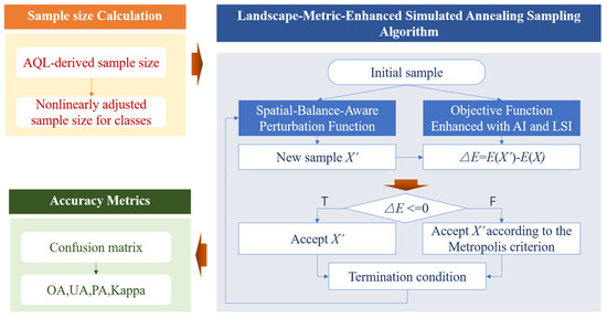
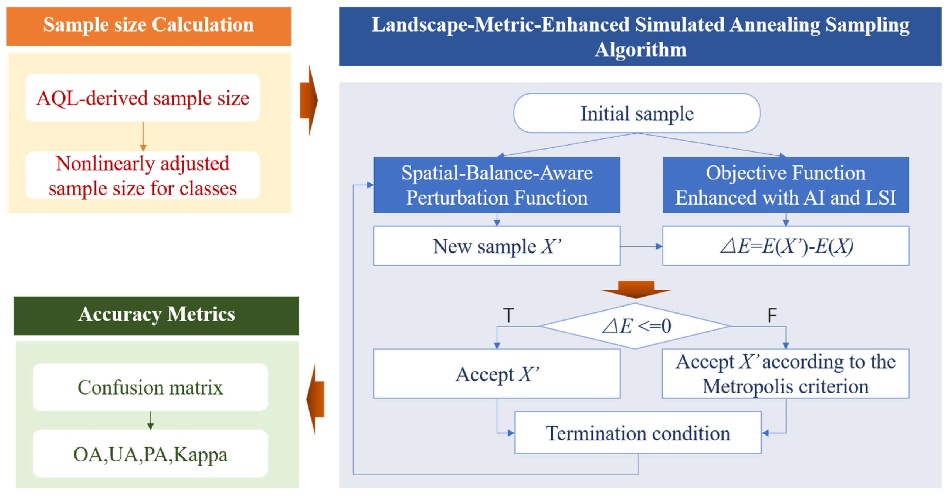
To achieve multi-objective optimization that accounts for both landscape heterogeneity and the spatial balance of samples, we propose a landscape-metric-enhanced simulated annealing sampling algorithm. The principal improvements comprise a spatial-balance-aware perturbation function, an energy function that incorporates landscape metrics, and a termination condition. The technical workflow is shown in Figure 1.

Figure 1. Technical workflow.

2.2.1. Spatial-Balance-Aware Perturbation Function

In conventional simple random perturbation strategies, the perturbation magnitude is generally either fixed or determined by a straightforward random step. Since this approach cannot be dynamically adjusted to the current state, it may lead to inefficient exploration of the solution space and can even result in invalid searches. To address this issue, the proposed algorithm introduces an adaptive perturbation magnitude, a feasible region constraint, and a maximum number of attempts to enhance the spatial balance of the sample distribution.

(1) Adaptive perturbation magnitude

The perturbation magnitude refers to the maximum allowable displacement (step length) between a new solution and the current solution in the solution space. It governs the step length of the neighborhood search and determines the magnitude of the random displacement of candidate solution X′ relative to the current solution X, specifically the order of |X′ − X|.

In our approach, we implement a neighborhood generation strategy where the perturbation magnitude ΔX of the new solution is not fixed; instead, its random interval is adaptively adjusted based on the algorithm’s state. Under this strategy, ΔX decreases more gradually with the current temperature T, facilitating large-scale exploration during most stages and transitioning to a fine search only once T falls below a certain threshold. This methodology maintains perturbation diversity, broadens the search range within the solution space, and reduces the risk of convergence to a local optimum.

Let X denote the coordinates of the current solution and X′ those of the perturbed solution. Their relationship is expressed as:

$$X^{\prime }=X+\Delta X \Delta X\in [-{\mathrm{R}}_0{\left({\displaystyle \frac{T_{k+1}}{T_k}}\right)}^k,{\mathrm{R}}_0{\left({\displaystyle \frac{T_{k+1}}{T_k}}\right)}^k]$$

(3)

Here, ${\mathrm{R}}_0$ represents the initial perturbation radius, while $T_k$ denotes the current temperature at iteration $k$. $\Delta X$ is a random variable drawn from a specified distribution within a defined interval, which establishes the limits and distribution of $\Delta X$. In the early iterations, a broad interval allows for quick coverage of the solution space, helping to identify promising areas. During the later iterations, a narrow interval facilitates a more refined search within those regions, enabling the accurate identification of the optimal solution.

(2) Feasible-region constraint

To ensure that each generated solution is admissible, a feasible-region constraint operator is incorporated into the perturbation function. A newly generated sample must lie within the valid region and must not duplicate any existing sampling point. This constraint guarantees that new solutions generated during the perturbation process are valid, thereby preventing the occurrence of infeasible or duplicate solutions. The feasible-region constraint C is expressed as:

$$C=max(L,min(X^{\prime },U\left)\right)$$

(4)

$X^{\prime }$ represents the newly generated candidate solution or the perturbed variable value. The value of $X^{\prime }$ is constrained within the closed interval [$L$,$U$], where $L$ denotes the lower bound and $U$ denotes the upper bound. In this paper, $L$ and $U$ refer to the boundaries of the experimental area.

(3) Maximum number of attempts

The inner loop of simulated annealing algorithm repeatedly executes the sequence “generate a new solution through perturbation → calculate the energy difference → apply the Metropolis criterion”, while maintaining a constant current temperature T. To enhance the stability of the perturbation strategy, we introduce a maximum number of attempts, denoted as K_max. If a valid solution cannot be generated within this limit, the current perturbation process is terminated, thereby preventing infinite loop and improving computational efficiency.

The maximum number of attempts is generally proportional to the sample size n:

$$K_{max}=t·n$$

(5)

The proportionality coefficient t is an empirical constant. A larger value of t leads to more thorough search, but also results in longer computation time; a smaller value of t enables faster calculation, but the algorithm may fall into a local optimum. In this paper, t is defined as a multiple of 10, which is set to 1, 3 and 5 times for low, medium and high heterogeneity partitions espectively, so as to ensure stable convergence even under complex landscape indices.

In summary, the perturbation function in the landscape-metric-enhanced simulated annealing algorithm is:

$$X^{\prime }=C\left\{X+\Delta X \Delta X\in [-{\mathrm{R}}_0{\left({\displaystyle \frac{T_{k+1}}{T_k}}\right)}^k,{\mathrm{R}}_0{\left({\displaystyle \frac{T_{k+1}}{T_k}}\right)}^k]\right\} (K_{max}=t·n)$$

(6)

2.2.2. Objective Function Enhanced with AI and LSI

(1) Base energy function

To address the landscape heterogeneity of mapped classes, we stratify the validation area into high-, medium-, and low-heterogeneity regions based on the heterogeneity represented in the data. Fixed weights in the energy function are subsequently replaced with dynamic weights assigned according to the differences in heterogeneity among strata. This adjustment increases the emphasis placed on highly heterogeneous regions during the optimization process.

We examine the Aggregation Index (AI) and Landscape Shape Index (LSI) for geographic stratification by landscape heterogeneity and evaluate the suitability of the two landscape metrics.

The Aggregation Index ($AI$) measures the degree to which landscape patches are spatially aggregated. It quantifies whether patches of a land-cover class are clustered or dispersed in space and is calculated as follows:

$$AI=\left({\displaystyle \frac{g_i}{g_{max,i}}}\right)\times 100$$

(7)

where g_i is the length of boundaries shared by pixels of the same class within a patch; g_max,i is the corresponding boundary length when patch aggregation is maximized; and AI represents the degree of aggregation of a land-cover class, ranging from 0 to 100.

The Landscape Shape Index ($LSI$) measures the shape complexity of landscape patches and primarily characterizes their boundary configuration and geometric complexity. It is calculated as:

$$LSI={\displaystyle \frac{E}{4\sqrt{A}}}$$

(8)

where E is the total boundary length of the patches, typically measured in pixel or grid units, and A is their total area, measured in grid-cell area units. Because the standard LSI has no fixed upper bound, it is normalized to the interval 0–1 to facilitate statistical analysis. The normalized $LSI$ is calculated as:

$${LSI}^{\prime }={\displaystyle \frac{LSI-1}{LS{I}_{\mathrm{m}\mathrm{a}\mathrm{x}}-1}}$$

(9)

where $LS{I}_{\mathrm{m}\mathrm{a}\mathrm{x}}$ is the maximum LSI value among all patches in the study area.

Based on the classification criteria specified in Table 1, a simple stratification process was implemented for all land classes. The stratification process first adopts the natural breakpoint method to complete the preliminary clustering division. To enhance the engineering practicability and operational convenience, the initially calculated non-integer stratification thresholds are manually adjusted to the nearest rounded integers, without altering the inherent sample distribution characteristics of each stratum.

Table 1. Landscape-heterogeneity strata based on AI and normalized LSI.

Landscape-Heterogeneity Stratum	AI	LSI′	w
High	0–50	0.8–1.0	$w_h$
Medium	50–80	0.5–0.8	$w_m$
Low	80–100	0–0.5	$w_l$

Within each stratum, the weight is determined from the standard deviation of the landscape metric:

$$\mathrm{w}=\sqrt{{\displaystyle \frac{1}{m}}{\sum }_{i=1}^m{(LI-\overline{LI})}^2}(LI=AI or LI={LSI}^{\prime })$$

(10)

LI denotes the landscape metric, either AI or LSI′ in this study, and m is the number of moving windows within the geographic stratum. After the weights have been determined, the base energy function becomes:

$$E\left(S\right)=w_{h}C\left(X_h\right)+w_{m}C\left(X_m\right)+w_{l}C\left(X_l\right)+w_{d}D\left(X_T\right)$$

(11)

$X$ is the sample set; $X_h$, $X_m$, and $X_l$ are the corresponding solutions in the high-, medium-, and low-heterogeneity strata, respectively. $C\left(X\right)$ is a spatial clustering metric for the set of sampling points. It quantifies the evenness of their spatial dispersion; a smaller value indicates a more uniform distribution and a higher-quality sampling design.

$$\mathrm{C}(X)={\sum }_{i=1}^N{\sum }_{j=i+1}^N{\displaystyle \frac{1}{d_{ij}^2}}$$

(12)

d_ij is the Euclidean distance between the ith and jth sampling points. $D\left(X\right)$ is the global coverage-error metric, defined as:

$$D\left(X\right)={\sum }_{i=1}^u{d}_i$$

(13)

m is the total number of grid cells into which the study area is divided, and d_i is the Euclidean distance from the center of the ith grid cell to its nearest sampling point. The target area within the experimental zone is partitioned into equal-area grids, and m is strictly equal to the preset sample size.

(2) Sample-size penalty term

To ensure that the number of samples in each region reaches its prescribed target, a penalty term for sample-size deviation is added to the energy function. This term guides the optimization toward a better global solution while promoting a more uniform spatial distribution and stronger regional represent ativeness.

$R$ is the number of strata into which the study area is divided. $n_r$ is the actual number of sampling points in the rth region under the current design, and $N_r^{target}$ is the prescribed target number of samples for that region.

$${\mathrm{P}}_{\mathrm{b}\mathrm{a}\mathrm{l}\mathrm{a}\mathrm{n}\mathrm{c}\mathrm{e}}\left(\mathrm{X}\right)={\sum }_{r=1}^R{(n_r-N_r^{target})}^2$$

(14)

(3) Spatial-balance penalty term

To improve the uniformity of the spatial distribution, the sum of the inverse squared nearest-neighbor distances is introduced into the energy function as a penalty term. This mechanism penalizes excessive spatial concentration and therefore produces a more even distribution of sampling points.

$$P_{nn}(\mathrm{S})={\sum }_{i=1}^n{\displaystyle \frac{1}{d_{min,i}^2+\epsilon }}$$

(15)

Here, $n$ is the number of samples, $d_{min,i}$ is the Euclidean distance from the $i$th point to its nearest neighbor, and $\epsilon$ is a small positive constant that prevents a zero denominator and numerical overflow when two points coincide.

The energy function of the AI/LSI-enhanced simulated annealing sampling algorithm is therefore summarized as:

$$E\left(S\right)=w_{h}C\left(S_h\right)+w_{m}C\left(S_m\right)+w_{l}C\left(S_l\right)+w_{d}D\left(S_T\right)+{\lambda }_1{P}_{nn}\left(S_T\right)+{\lambda }_2{\mathrm{P}}_{\mathrm{b}\mathrm{a}\mathrm{l}\mathrm{a}\mathrm{n}\mathrm{c}\mathrm{e}}\left(S_T\right)$$

(16)

2.2.3. Termination Condition

To reduce the number of algorithm iterations, this paper proposes a flexible termination condition, which mainly includes the following three parts.

First, maximum consecutive rejection count: If no better sample solution is found within a specified number of attempts, the algorithm stops automatically. This prevents the algorithm from falling into useless solution spaces, saving computing power and accelerating convergence.

Second, non-improvement count: If the sample solution does not show any improvement within a certain number of iterations, the algorithm stops in advance. This avoids unnecessary continuous operation after convergence and saves computing resources.

Third, energy change threshold: An extremely small value is introduced as the energy change threshold. When the difference between the energy of the current solution and the optimal solution is smaller than this threshold, the algorithm is considered to have converged. This convergence condition ensures optimization accuracy while effectively avoiding excessive computation.

Apart from the traditional maximum iteration number judgment, this paper combines multiple conditions including energy change, rejection count and non-improvement count to jointly determine the convergence timing. This multi-condition convergence strategy allows the algorithm to flexibly adjust the stop timing, which not only ensures sufficient algorithm operation, but also prevents invalid computation. This study determines three core termination control parameters of the simulated annealing algorithm through multiple sets of repeated controlled verification experiments: the maximum consecutive rejection count is set to 50, the non-improvement count is set to 30, and the energy change threshold is set to 0.1.

2.3. Accuracy Metrics

Reference labels are collected through expert interpretation of high-resolution imagery. For a mixed pixel, the land-cover class that occupies the largest area is designated as the primary class. Samples are used to construct the confusion matrix and calculate the accuracy metrics. Classification accuracy is evaluated from the confusion matrix using weighted overall accuracy ($\widehat{OA}$), user’s accuracy (UA), producer’s accuracy (PA), and the kappa coefficient. Let the confusion matrix contain C classes, let n_ij denote the number of samples classified as class i with a reference class is j and let N represent the total number of samples. Due to significant differences in the sampling probabilities of different land cover classes, this study employs a weighted overall accuracy ($\widehat{OA}$) calculation based on the area proportion of land cover types to eliminate the interference of sample distribution bias on the accuracy assessment results. This method involves the ratio of the diagonal elements ($n_{ii}$) to the sum of the elements in that row, weighted by the area proportion (${\mathrm{w}}_{\mathrm{i}}$) of the respective land cover type.

$$\widehat{OA}={\displaystyle {\sum }_{i=1}^C}{\mathrm{w}}_{\mathrm{i}}{\displaystyle \frac{n_{ii}}{{\displaystyle {\sum }_{j=1}^C}{n}_{ij}}}$$

(17)

The user’s accuracy for class i is the proportion of samples classified as class i that actually belong to that class and is calculated as:

$${UA}_i={\displaystyle \frac{n_{ii}}{{\displaystyle {\sum }_{j=1}^C}{n}_{ij}}}$$

(18)

The producer’s accuracy for class i is the proportion of reference samples that belong to class i and are classified correctly and is calculated as:

$${PA}_i={\displaystyle \frac{n_{ii}}{{\displaystyle {\sum }_{j=1}^C}{n}_{ji}}}$$

(19)

The kappa coefficient measures agreement between the classification and the reference data after accounting for chance agreement and is calculated as:

$$\kappa ={\displaystyle \frac{{\sum }_{i=1}^m{n}_{ii}-{\sum }_{i=1}^m{n}_{+i}{n}_{i+}}{1-{\sum }_{i=1}^m{n}_{+i}{n}_{i+}}}$$

(20)

3. Experiments

3.1. Study Area and Data

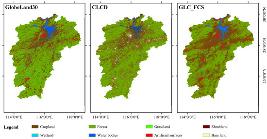
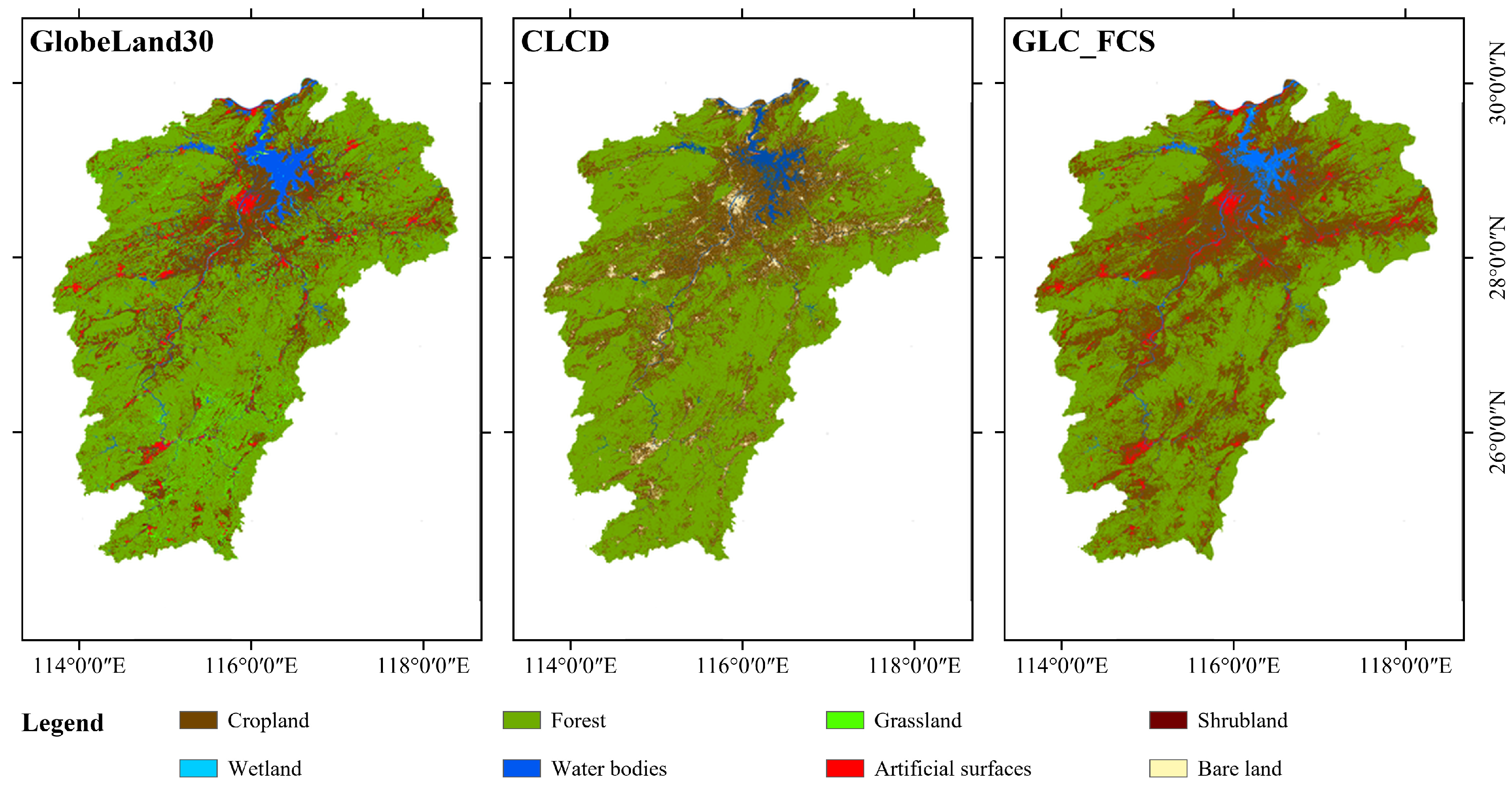
Jiangxi Province is located in southeastern China, near the middle and lower reaches of the Yangtze River. Its terrain consists mainly of mountains, hills, and plains, characterized by diverse ecological landscapes and an extensive river network. For our analysis, we utilized three land-cover products for the year 2020: GlobeLand30, CLCD, and GLC_FCS. The spatial distributions of these products are illustrated in Figure 2. Forest cover is the dominant class, primarily concentrated in the mountainous regions of eastern, southern, and western Jiangxi. This distribution aligns with the regional topographic pattern, where higher elevations are found in the southeast and lower elevations in the northwest. Cropland is predominantly located in the plains of central and northern Jiangxi, including the Poyang Lake Plain.

Figure 2. Spatial distributions of the three land-cover products in Jiangxi Province.

This study conducts two sets of controlled experiments across the full jurisdiction of Jiangxi Province to compare the proposed method with selected sampling methods and assess its performance across three land-cover products. In the first experiment, the improved simulated annealing sampling method optimized by LSI and AI heterogeneity zoning is applied to carry out independent accuracy evaluation on GlobeLand30, CLCD and GLC_FCS. The consistency of performance across different datasets is analyzed to verify the universality and robustness of the proposed method when applied to different data sources. In the second experiment, five sampling methods, namely simple random sampling, systematic sampling, spatial balanced sampling, traditional simulated annealing sampling, and the proposed improved simulated annealing sampling optimized by landscape heterogeneity zoning, are adopted to generate sample sets—GlobeLand30. The accuracy reliability of different sampling schemes is compared to verify the performance advantages of the improved simulated annealing sampling method. The sample size is 1778, with a 95% confidence interval and a relative error of 0.1.

3.2. Experiments on Multiple Datasets

3.2.1. Sampling Results Optimized by LSI and AI

(1) Sample Size Calculation

GlobeLand30 and CLCD both adopt a completely consistent classification system for land cover products, encompassing ten land cover types: cultivated land, forest land, grassland, shrubland, wetland, water bodies, tundra, artificial surfaces, bare land, and permanent ice and snow. The original GLC_FCS data uses the LCCS secondary classification standard, which includes 30 subcategories. To achieve comparability among the three products in the Jiangxi Province research area, this study employs semantic mapping of land cover types and attribute aggregation methods to convert the 30 subcategories of GLC_FCS into a unified classification system of 10 benchmark categories that completely matches those of GlobeLand30 and CLCD, thereby eliminating differences in land cover definitions among different products. After achieving this unified land cover classification system, the statistical results of the land cover area for the three products in Jiangxi Province are fully presented in Table 2, which can provide fundamental data support for subsequent sampling method probability calculations and area-weighted overall accuracy derivations. GlobeLand30 covers 8 land cover types. Due to the highly fragmented nature of wetland patches in Jiangxi Province, the CLCD product overlooked wetland during the classification production process; GLC_FCS, when converting across classification systems, missed the bare land type. Ultimately, both products only contain 7 land cover types in Jiangxi Province. All three products indicate that cropland and forests are the main categories, accounting for 85% to 90% of the total area. Grassland, shrubland, wetland, and bare land have a very small coverage area in Jiangxi Province, with each type accounting for less than 1% of the total area in different datasets.

Table 2. Sample-size calculations for the three land-cover products.

	GlobeLand30		CLCD		GLC_FCS
Class	Area Proportion (%)	Sample Size	Area Proportion (%)	Sample Size	Area Proportion (%)	Sample Size
Cropland	27.67	456	29.26	547	31.66	531
Forest	59.43	669	63.40	805	59.10	726
Grassland	2.99	150	0.01	12	0.01	7
Shrubland	1.47	106	0.03	19	1.17	102
Wetland	0.01	13	0.00	0	0.16	37
Water	4.33	180	3.42	187	3.64	180
Artificial surfaces	3.99	175	0.01	9	4.27	195
Bare land	0.11	29	3.87	199	0.00	0

Using Formula (2), the sample size for each category was calculated, with results shown in Table 2. If samples were allocated based on area proportion or equal-area geographical stratification, these categories might only receive one or even no samples, a phenomenon that will be thoroughly validated in the subsequent second control experiment. After conducting nonlinear adjustments, sufficient sample sizes were obtained even for grassland, shrubland, and wetland, allowing for the estimation of user and producer accuracy.

(2) Analysis of Spatial Sampling Optimization

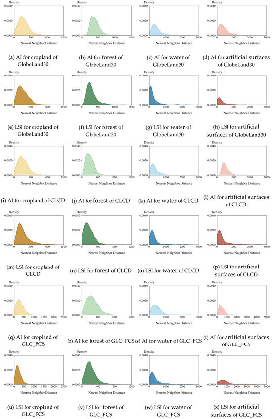
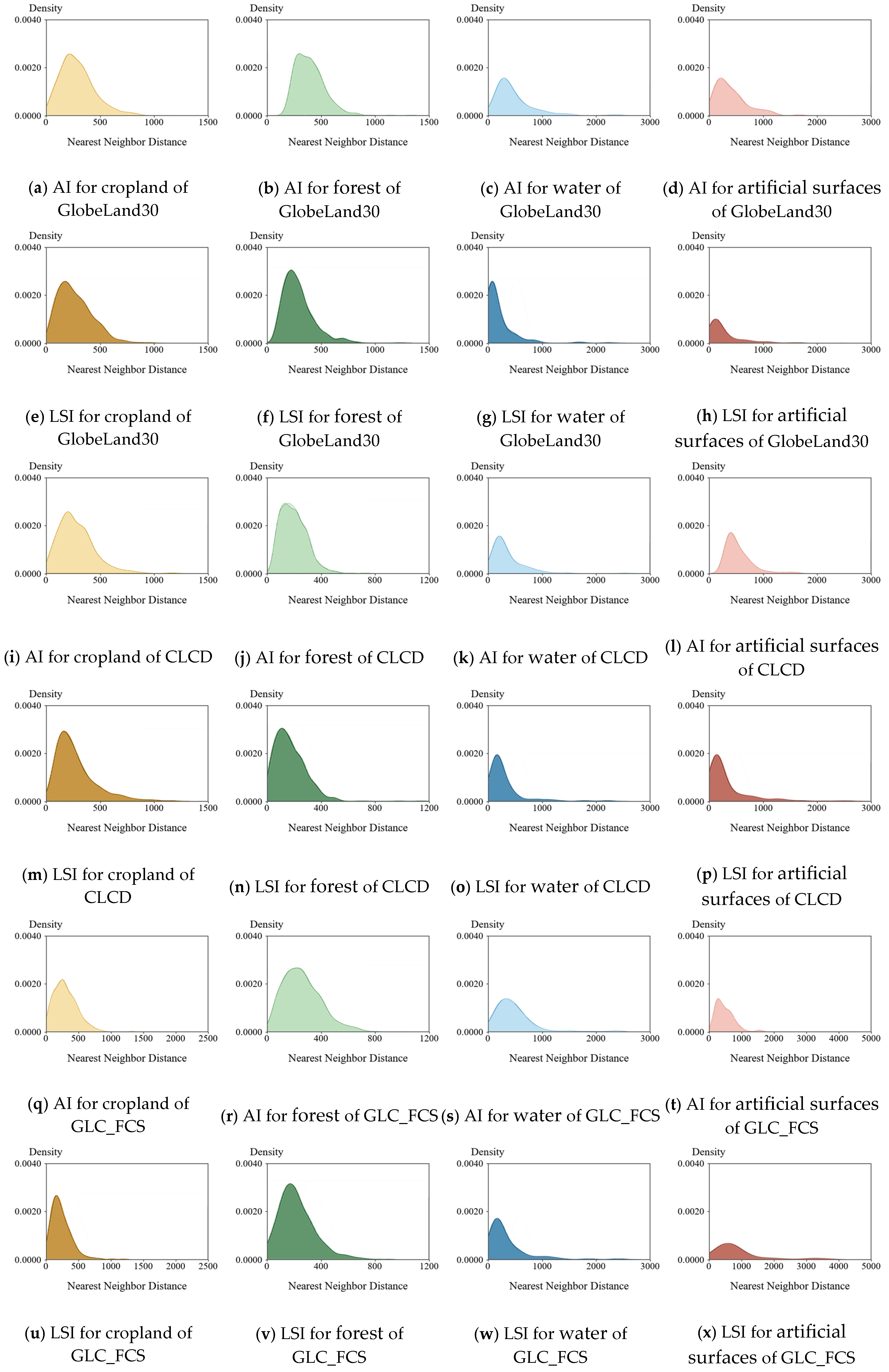
The AI and LSI were applied separately to generate two sets of samples for each of the GlobeLand30, CLCD, and GLC_FCS land-cover products. The kernel density estimation (KDE) curves for the AI- and LSI-optimized sample distributions are shown in Figure 3. Among all classes, cropland and forest are widely distributed and highly continuous matrix classes, while water bodies and artificial surfaces occupy smaller areas and exhibit more complex shapes. Consequently, these four classes were chosen as representative examples for further analysis.

Figure 3. Kernel density estimation curves.

For both sample sets of the three products, the KDE curves for the four representative classes exhibit a general leftward shift, indicating that the optimized samples are more concentrated in highly heterogeneous areas. This concentration enhances the ability to capture land cover characteristics in complex regions. Pairwise comparison of the AI- and LSI-based KDE curves reveal that the profiles under LSI optimization are narrower and more concentrated for all four classes across all three products. This suggests that LSI optimization allocates a higher density of samples to highly heterogeneous areas and places greater emphasis to regions with complex boundary shapes.

3.2.2. GlobeLand30 Accuracy Assessment

To verify the reference labels of the sampled points, we utilized contemporaneous Sentinel-2 imagery with a spatial resolution of 10 m. For difficult samples in the Sentinel-2 imagery where land cover boundaries are ambiguous and cannot be clearly identified, we further conducted a secondary manual review and interpretation using high-resolution historical images from Google Earth.

Table 3 and Table 4 present the confusion matrices for GlobeLand30 based on samples optimized using AI and LSI, respectively. In Table 4, cropland, forest, and water body are classified relatively accurately, while grassland and shrubland exhibit high of misclassification rates. Significant confusion is observedbetween forest and cropland, as well as between grassland and shrubland. Grassland is particularly susceptible to misclassification, with 72 samples classified incorrectly as forest.

Table 3. Confusion matrix for GlobeLand30 based on AI-optimized samples.

Class	Cropland	Forest	Grassland	Shrubland	Wetland	Water	Artificial Surfaces	Bare Land	Total	User’s Accuracy (UA)
Cropland	392	45	8	3	6	2	0	0	456	85.96%
Forest	1	641	14	7	0	5	1	0	669	95.81%
Grassland	6	72	60	7	0	0	5	0	150	40.00%
Shrubland	5	48	0	53	0	0	0	0	106	50.00%
Wetland	2	0	0	0	8	3	0	0	13	61.54%
Water	8	6	4	0	5	148	0	9	180	82.22%
Artificial surfaces	16	8	1	2	0	0	143	5	175	81.71%
Bare land	4	1	0	0	1	0	4	19	29	65.52%
Total	434	821	87	72	20	158	153	33	1778	—
Producer’s accuracy (PA)	90.32%	78.08%	68.97%	73.61%	40.00%	93.67%	93.46%	57.58%	—	—

Table 4. Confusion matrix for GlobeLand30 based on LSI-optimized samples.

Class	Cropland	Forest	Grassland	Shrubland	Wetland	Water	Artificial Surfaces	Bare Land	Total	User’s Accuracy (UA)
Cropland	382	49	10	6	7	2	0	0	456	83.77%
Forest	3	637	14	9	0	6	0	0	669	95.22%
Grassland	6	64	70	4	0	0	5	1	150	46.67%
Shrubland	6	38	0	60	0	0	0	2	106	56.60%
Wetland	2	0	0	0	7	4	0	0	13	53.85%
Water	8	6	4	0	5	148	0	9	180	82.22%
Artificial surfaces	13	12	4	2	0	0	134	10	175	76.57%
Bare land	4	3	0	0	2	0	5	15	29	51.72%
Total	424	809	102	81	21	160	144	37	1778	—
Producer’s accuracy (PA)	90.09%	78.74%	68.63%	74.07%	33.33%	92.50%	93.06%	40.54%	—	—

Table 4 also demonstrates strong classification performance for cropland, forest, and water, while the accuracy for grassland, shrubland, wetland, and bare land remains relatively low. Significant confusion is observed between cropland and either forest or grassland, as well as between forest and grassland, and between forest and shrubland.

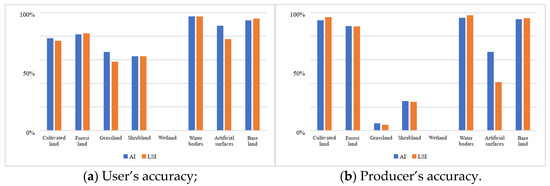
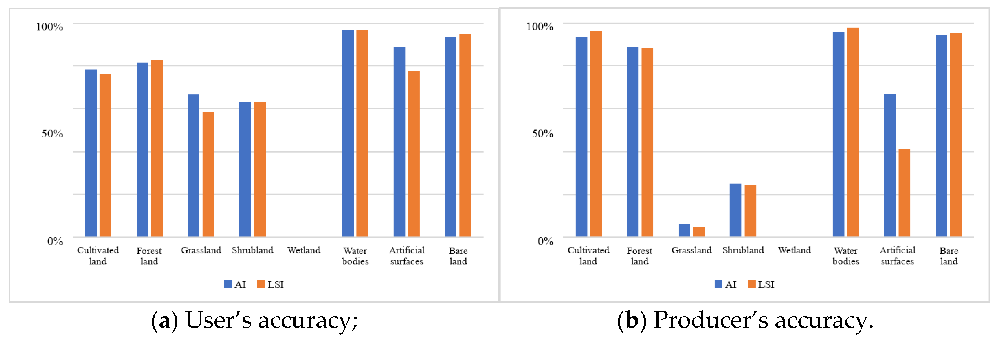
Figure 4 compares the user’s and producer’s accuracies derived from the AI- and LSI-optimized samples. Both sample sets yield very similar assessment results for GlobeLand30. The producer’s accuracies for cropland, forest, grassland, shrubland, water, and artificial surfaces are nearly identical, with a more significant difference observed only for bare land. In terms of user’s accuracy, the differences for cropland and fores-which cover the largest areas are minimal, and the discrepancies for the other classes remain minor; bare land again exhibits the largest difference. The areas classified as bare-land areas possess fragmented and complex surface and terrain characteristics. If insufficient samples are allocated to this class, local extremes may be easily be overlooked, leading to greater variability in the resulting accuracy estimates.

Figure 4. User’s and producer’s accuracies of GlobeLand30.

3.2.3. CLCD Accuracy Assessment

Table 5 and Table 6 display the confusion matrices for the CLCD based on AI- and LSI-optimized samples. In Table 6, the CLCD demonstrates more accurate classification for water and bare land compared to GlobeLand30, but exhibits higher misclassification rates for forest and grassland. Misclassified samples are spread across several classes, with notable occurrences in grassland (98 samples) and shrubland (21 samples). It is worth noting that wetland is excluded from the CLCD product.

Table 5. Confusion matrix for CLCD based on AI-optimized samples.

Class	Cropland	Forest	Grassland	Shrubland	Wetland	Water	Artificial Surfaces	Bare Land	Total	User’s Accuracy (UA)
Cropland	428	79	25	10	0	0	0	5	547	78.24%
Forest	21	657	98	21	0	8	0	0	805	81.61%
Grassland	1	2	8	1	0	0	0	0	12	66.67%
Shrubland	1	1	2	12	0	0	0	3	19	63.16%
Wetland	0	0	0	0	0	0	0	0	0	—
Water	0	0	0	4	0	181	0	2	187	96.79%
Artificial surfaces	0	0	0	0	0	0	8	1	9	88.89%
Bare land	6	3	0	0	0	0	4	186	199	93.47%
Total	457	742	133	48	0	189	12	197	1778	—
Producer’s accuracy (PA)	93.65%	88.54%	6.02%	25.00%	—	95.77%	66.67%	94.42%	—	—

Table 6. Confusion matrix for CLCD based on LSI-optimized samples.

Class	Cropland	Forest	Grassland	Shrubland	Wetland	Water	Artificial Surfaces	Bare Land	Total	User’s Accuracy (UA)
Cropland	417	85	26	18	0	0	0	1	547	76.23%
Forest	12	665	106	14	0	4	4	0	805	82.61%
Grassland	1	2	7	1	0	0	0	1	12	58.33%
Shrubland	1	1	3	12	0	0	0	2	19	63.16%
Wetland	0	0	0	0	0	0	0	0	0	—
Water	0	0	0	3	0	181	0	3	187	96.79%
Artificial surfaces	0	0	0	0	0	0	7	2	9	77.78%
Bare land	2	1	0	1	0	0	6	189	199	94.97%
Total	433	754	142	49	0	185	17	198	1778	—
Producer’s accuracy (PA)	96.30%	88.20%	4.93%	24.49%	—	97.84%	41.18%	95.45%	—	—

The results presented in Table 6 are consistent with those in Table 5. Water and bare land continue to be classified accurately, while grassland and shrubland show poor performance. Out of 187 water samples, 181 are correctly classified, yielding an accuracy of 96.8% which represents the best performance among all classes. Classification confusion is observed between forest and grassland.

Figure 5 compares the user’s and producer’s accuracies for the two CLCD sample sets. The AI- and LSI-optimized samples yield highly consistent results in the accuracy assessment of the CLCD. With the exception of artificial surfaces, the user’s and producer’s accuracies for every class are very similar across the two sets. Artificial surfaces constitute a very small proportion of the CLCD dataset. Although the nonlinear adjustment strategy increases their sample size, significant differences in spatial distribution remain between the AI- and LSI-optimized samples. The LSI approach places greater emphasis on class boundaries, where mixed pixels are concentrated, directly resulting in lower accuracy estimates for the LSI-optimized samples compared to the AI-optimized samples.

Figure 5. User’s and producer’s accuracies of CLCD.

3.2.4. GLC_FCS Accuracy Assessment

Table 7 and Table 8 present the confusion matrices for GLC_FCS based on AI- and LSI-optimized samples. In Table 7, GLC_FCS demonstrates greater accuracy in classifying wetland and artificial surfaces compared to other products, while its performance regarding cropland and forest is on par with that of CLCD. Among the cropland samples, 81 are misclassified as forest and 19 as shrubland, indicating a slightly lower performance relative to CLCD. In Table 8, GLC_FCS shows relatively strong performance for shrubland and artificial surfaces, although its accuracy for wetland is reduced. Of the 37 wetland samples, 24 are correctly classified, yielding an accuracy rate of 64.9%.

Table 7. Confusion matrix for GLC_FCS based on AI-optimized samples.

Class	Cropland	Forest	Grassland	Shrubland	Wetland	Water	Artificial Surfaces	Bare Land	Total	User’s Accuracy (UA)
Cropland	405	81	14	19	0	0	12	0	531	76.27%
Forest	24	603	61	29	0	1	8	0	726	83.06%
Grassland	0	1	6	0	0	0	0	0	7	85.71%
Shrubland	2	6	12	81	0	0	1	0	102	79.41%
Wetland	0	0	1	2	26	8	0	0	37	70.27%
Water	0	0	0	4	12	164	0	0	180	91.11%
Artificial surfaces	17	4	0	0	0	0	174	0	195	89.23%
Bare land	0	0	0	0	0	0	0	0	0	—
Total	448	695	94	135	38	173	195	0	1778	—
Producer’s accuracy (PA)	90.40%	86.76%	6.38%	60.00%	68.42%	94.80%	89.23%	—	—	—

Table 8. Confusion matrix for GLC_FCS based on LSI-optimized samples.

Class	Cropland	Forest	Grassland	Shrubland	Wetland	Water	Artificial Surfaces	Bare Land	Total	User’s Accuracy (UA)
Cropland	411	74	20	12	0	0	14	0	531	77.40%
Forest	28	591	59	26	0	1	21	0	726	81.40%
Grassland	0	1	6	0	0	0	0	0	7	85.71%
Shrubland	2	2	11	87	0	0	0	0	102	85.29%
Wetland	0	0	0	4	24	9	0	0	37	64.86%
Water	0	0	1	8	14	157	0	0	180	87.22%
Artificial surfaces	10	8	6	0	0	0	171	0	195	87.69%
Bare land	0	0	0	0	0	0	0	0	0	—
Total	451	676	103	137	38	167	206	0	1778	—
Producer’s accuracy (PA)	91.13%	87.43%	5.83%	63.50%	63.16%	94.01%	83.01%	—	—	—

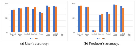
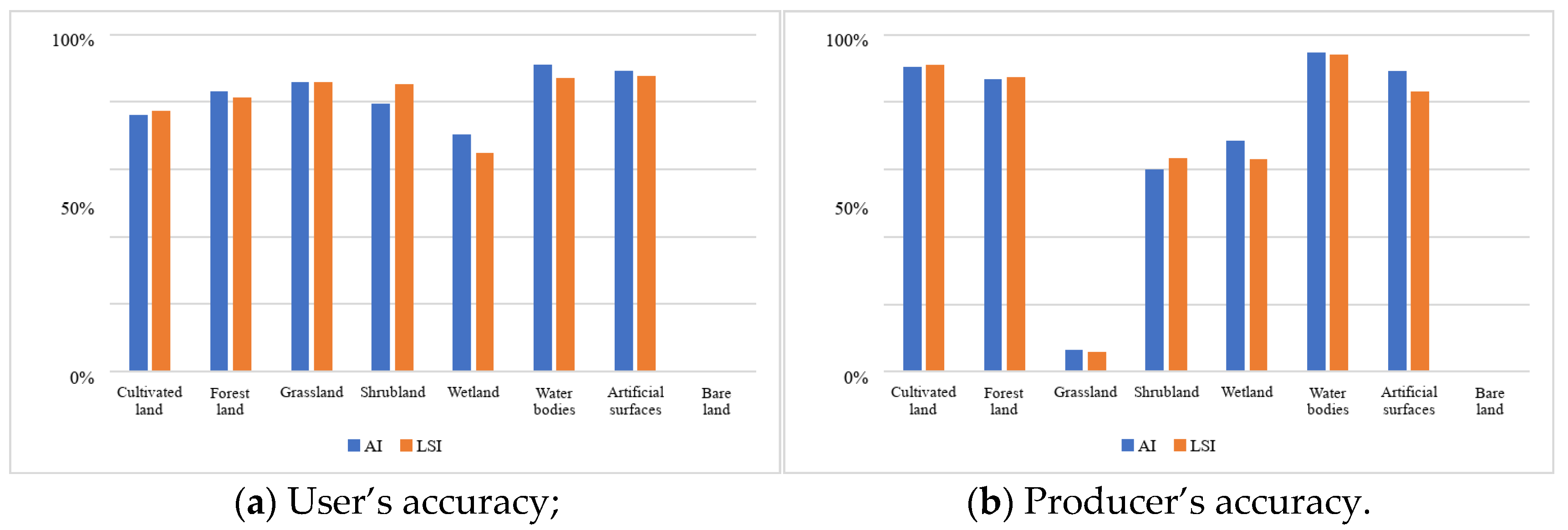
Figure 6 presents the accuracy-assessment results for GLC_FCS. The user’s and producer’s accuracies derived from both AI- and LSI-optimized sample sets are notably similar, with differences of less than 0.05 for most classes. Overall, the accuracy estimates from the LSI-optimized samples are slightly lower than those obtained from the AI-optimized samples.

Figure 6. User’s and producer’s accuracies of GLC_FCS.

3.2.5. Kappa Coefficient and Overall Accuracy Comparison

Table 9 reports the kappa coefficients and weighted overall accuracy ($\widehat{\mathrm{O}\mathrm{A}}$) values calculated from the confusion matrices. The weighted OA values ranged from 80.64% to 89.55%, and the kappa coefficients ranged from 0.749 to 0.763 across the three products and two sampling configurations. In Jiangxi Province, with $\widehat{\mathrm{O}\mathrm{A}}$ values of 82–83% and kappa coefficients between 0.75 and 0.76. For each product, the overall accuracy and kappa coefficient derived from the two sample sets are very similar. The difference in kappa is below 0.01 and differences in $\widehat{\mathrm{O}\mathrm{A}}$ is below 0.5 percentage points. These results highlight the high stability and consistency of the two optimized sample sets for assessing land-cover accuracy, thereby supporting the reliability of the experimental results.

Table 9. Kappa coefficients and overall accuracies for the three land-cover products.

Sample Set	Metric	GlobeLand30	CLCD	GLC_FCS
AI	Kappa coefficient	0.761	0.763	0.757
LSI		0.754	0.762	0.749
AI	$\widehat{\mathrm{O}\mathrm{A}}$ (%)	89.55	81.6	81.41
LSI		88.67	81.7	80.64

While the overall accuracies of the two sample sets are highly consistent, LSI optimization tends to favor transition zones between land-cover classes. These zones often contain numerous mixed pixels and are significantly more challenging to classify than homogeneous core areas. Consequently, both the kappa coefficient and $\widehat{\mathrm{O}\mathrm{A}}$ from the LSI-optimized samples are slightly lower than those from the AI-optimized samples. Nevertheless, the differences are minimal—below 0.01 for kappa and below 0.5 percentage points for $\widehat{\mathrm{O}\mathrm{A}}$—reflecting reasonable variation attributed to differing sampling preferences rather than indicating a change in the conclusion that the two sample sets provide highly consistent assessments.

3.2.6. User’s and Producer’s Accuracy Comparison

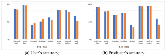
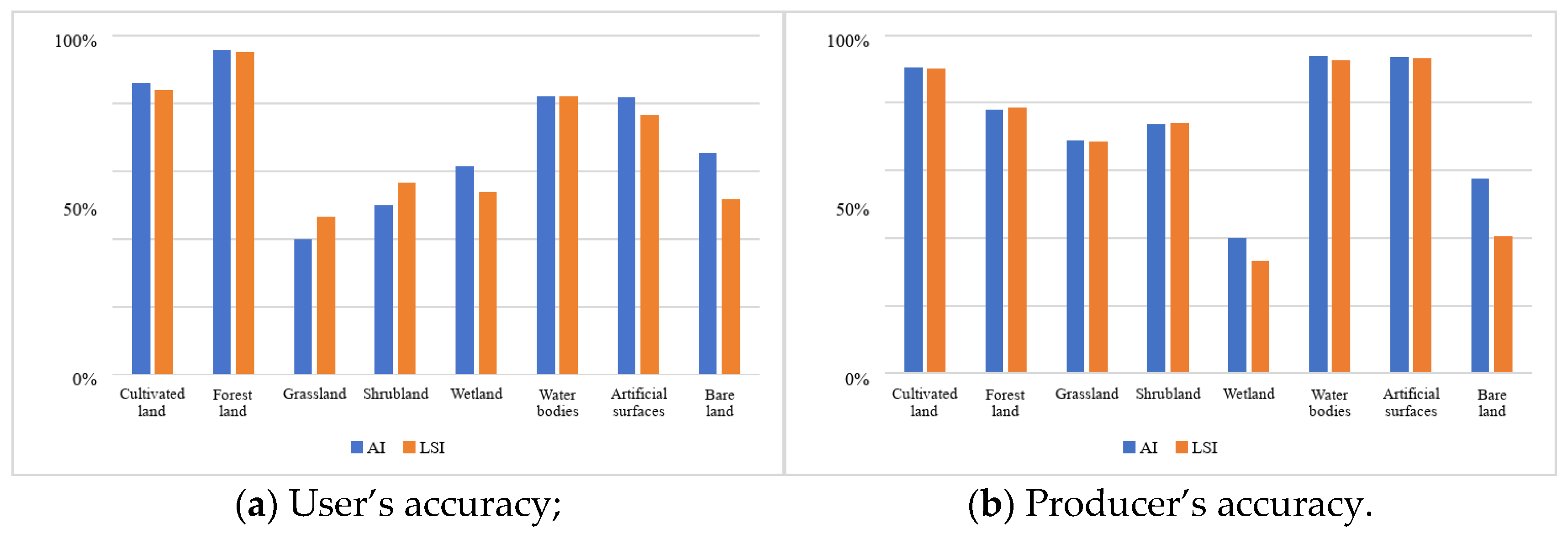
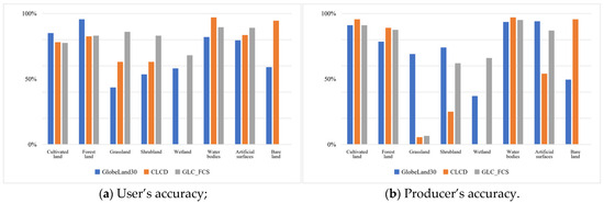
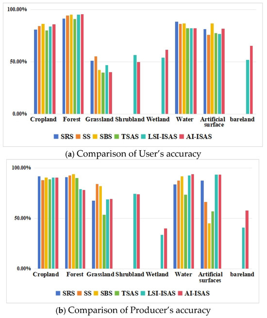
Averaging the assessment results from the two sample sets yields the user’s and producer’s accuracies for GlobeLand30, CLCD, and GLC_FCS shown in Figure 7. GlobeLand30 demonstrates strong performance for cropland, forest, water, and artificial surfaces. CLCD also exhibits high user’s and producer’s accuracies for cropland, forest, water, and bare land. Similarly, GLC_FCS performs well in cropland, forest, water, and artificial surfaces. For these classes, both user’s and producer’s accuracies are approximately 80%.

Figure 7. Mean user’s and producer’s accuracies.

All three products perform poorly for grassland, shrubland, and wetland. For GlobeLand30, the user’s and producer’s accuracies for these classes range only from 40% to 60%. CLCD shows user’s accuracies of approximately 60%, but its producer’s accuracies are below 25%, indicating particularly poor. For GLC_FCS, the user’s and producer’s accuracies for shrubland and wetland also fall within the range of 40% to 60%, while the producer’s accuracy for grassland is notably low.

3.3. Inter-Method Performance Comparison on GlobeLand30

Using GlobeLand30 as experimental data, simple random sampling (SRS), systematic sampling (SS), spatial balanced sampling (SBS), and traditional simulated annealing sampling (TSAS) were conducted in Jiangxi Province, followed by accuracy assessment. The comparison of the experimental results with LSI and AI improved simulated annealing sampling (ISAS) is as follows.

3.3.1. Comparison of Sampling Results

The summary of the sample quantities for each land type corresponding to the five sampling methods is detailed in Table 10. The statistical results show that the samples generated by the four traditional sampling methods are concentrated in the two dominant types, cultivated land and forest land, while the sample quantities for other land types are extremely low. In all sampling schemes, the number of samples for shrubland and wetlands is only 1 or even 0. The sample quantity for bare land is only 2 in simple random sampling, systematic sampling, and traditional simulated annealing sampling, while it is even 0 in spatial balanced sampling. The above sample sizes do not meet the calculation requirements for user accuracy and producer accuracy, leading to a significant deviation of their accuracy evaluation results from the actual classification errors, and they cannot provide reliable support for the accuracy verification of subsequent land cover products.

Table 10. Sample quantities for each class.

	SRS	SS	SBS	TSAS	ISAS
Cropland	488	484	479	459	456
Forest	1002	1019	1060	1058	669
Grassland	125	125	107	111	150
Shrubland	1	0	0	1	106
Wetland	0	0	2	0	13
Water	91	73	84	84	180
Artificial surfaces	69	75	46	63	175
Bare land	2	2	0	2	29
ALL	1778	1778	1778	1778	1778

3.3.2. User’s and Producer’s Accuracies

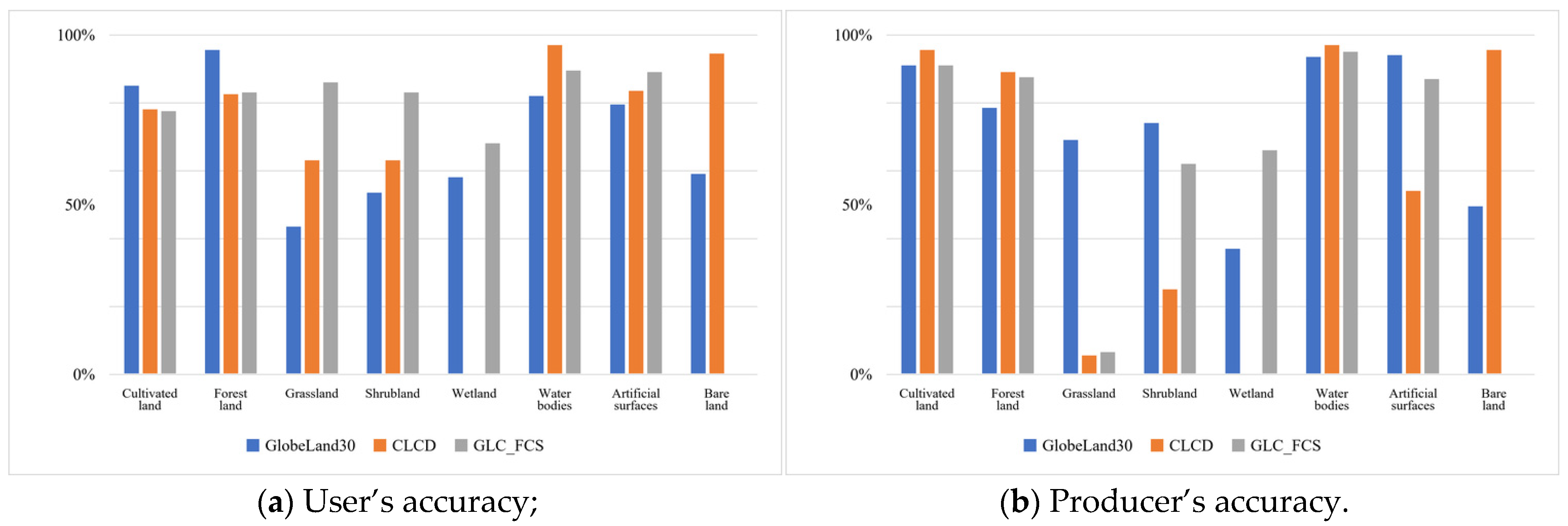
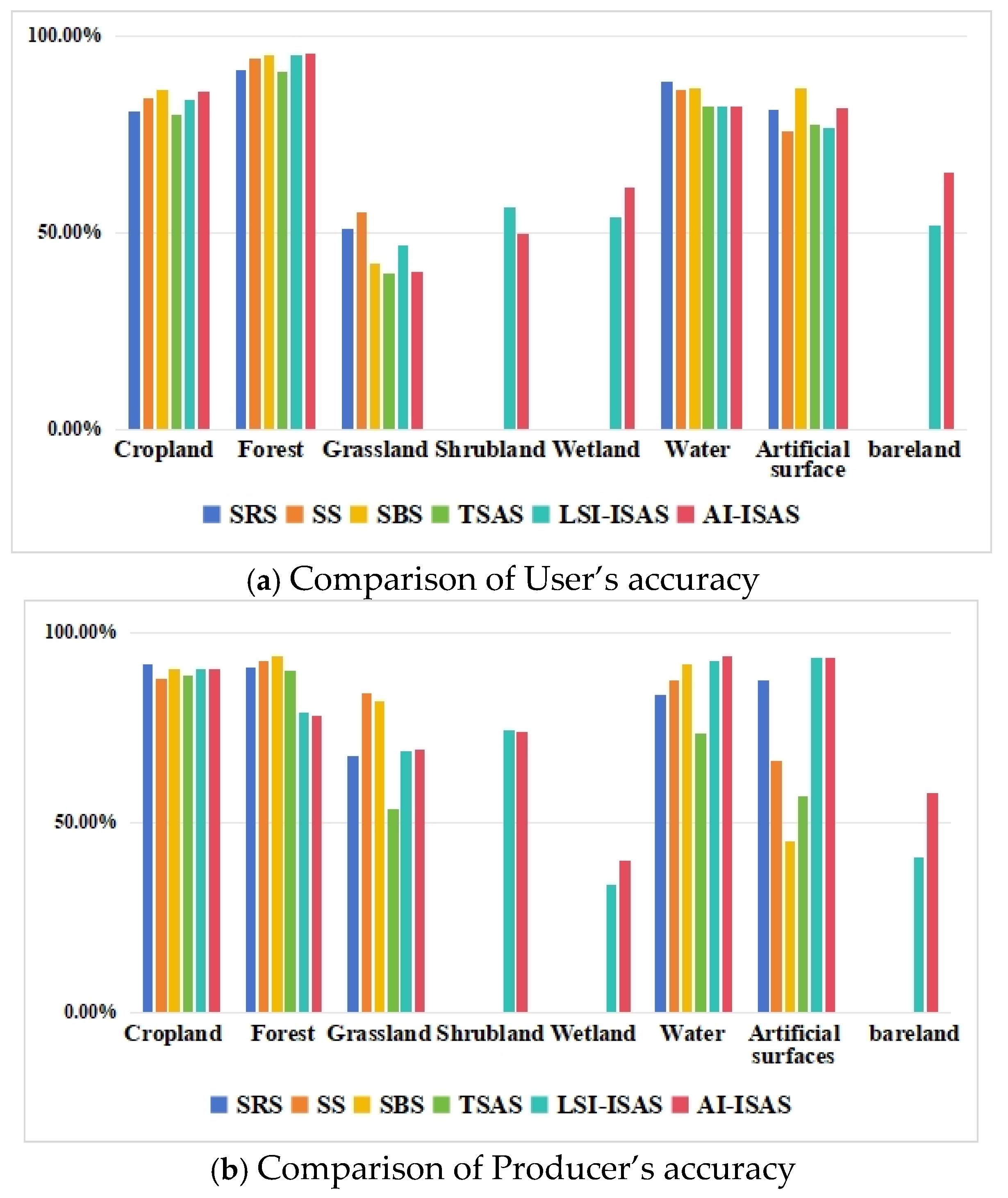
For the sample sets obtained from the four traditional sampling methods mentioned above, the same high-resolution remote sensing imagery was used as the visual interpretation data source to complete manual interpretation and land cover labeling. Based on the labeling results, the User’s Accuracy (UA) and Producer’s Accuracy (PA) for the four groups of samples were calculated, and these were compared with the UA and PA obtained from the LSI and AI-improved simulated annealing sampling method. The comparison chart is shown in Figure 8.

Figure 8. Comparison of user’s and producer’s accuracies.

In each sample set, the number of samples for cropland and forest land is sufficient, resulting in similar evaluation results for both categories. In the LSI-ISAS and AI-ISAS sample sets, the user accuracy (UA) and producer accuracy (PA) for cropland and forest land differ only slightly from those of other sample sets. The classification difficulty for water bodies is relatively low, and the UA and PA of the six sample sets are also similar, with the PA of the TSAS sample exhibiting a significantly low value. Grassland and artificial cover exhibit high fragmentation, and the number of distributed samples is limited, leading to considerable fluctuations in UA and PA across different sample sets. Specifically, for grassland, the difference in UA reaches 15%, with the grassland UA for LSI-ISAS and AI-ISAS samples being close to that of SBS and TSAS samples. The UA for artificial cover in LSI-ISAS and AI-ISAS samples is similar to that of SRS, SS, and TASA, while the SBS sample set shows the highest UA. The PA for artificial cover shows substantial variability, with only the SRS, LSI-ISAS, and AI-ISAS sample sets being similar.

In summary, the LSI-ISAS and AI-ISAS sample sets can complete the PA and UA assessments for all classifications without extreme high or low evaluation results. Other sample sets lack PA and UA assessments for three classifications and also show variations in UA and PA in the evaluations of grassland, water bodies, and artificial cover.

3.3.3. Kappa Coefficient and Overall Accuracy

The weighted overall accuracy and Kappa coefficients inferred from sample sets under different sampling strategies are summarized in Table 11, along with comparisons of the evaluation results of the improved sample sets optimized by LSI and AI. From the comparison results of OA, the differences in accuracy of the sample sets generated by the LSI-ISAS and AI-ISAS methods compared to the SBS method are controlled within 1%, and the differences with the SRS and SS methods do not exceed 2.5%; however, the weighted overall accuracy obtained by the TSAS method shows a difference of 5% compared to all the aforementioned methods. Under the condition that the total sample size reaches 1778, the weighted overall accuracy obtained by all sampling methods converges to the true value, and the overall differences between the different methods remain within a controllable range, indicating that the impact of the sampling methods on the weighted overall accuracy is relatively small.

Table 11. Comparison of $\widehat{\mathrm{O}\mathrm{A}}$ and Kappa coefficient.

	SRS	SS	SBS	TSAS	LSI-ISAS	AI-ISAS
Kappa coefficient	0.7833	0.7961	0.8065	0.716	0.754	0.761
$\widehat{\mathrm{O}\mathrm{A}}$ (%)	87.10%	87.79%	88.91%	83.52%	88.67%	89.55%

Further comparison of the Kappa coefficients obtained by different sampling methods reveals that the Kappa values for all methods fall within the range of 0.71 to 0.79, with the maximum difference not exceeding 0.1, indicating a high level of consistency overall. Similar to OA, the impact of sampling methods on the Kappa coefficient is also relatively low. Comparatively, the Kappa coefficients of the LSI-ISAS and AI-ISAS methods are at the median, while the Kappa coefficients obtained from the three traditional sampling methods SRS, SS, and SBS are slightly higher. This phenomenon may be attributed to the presence of five rare classes in the error matrices of LSI-ISAS and AI-ISAS, which have a relatively low sample proportion, whereas the SRS, SS, and SBS methods exhibit only two rare types due to the absence of shrubland, wetland and bareland classes. This structural difference in the matrices leads to a slight influence.

These results further confirm that the LSI-ISAS and AI-ISAS methods, while reducing the proportion of redundant samples in large areas of homogeneous distribution such as cultivated land and forest, simultaneously direct more samples to high fragmentation areas like grasslands, shrubs, wetlands, water bodies, and artificial covers. Due to the optimized spatial distribution characteristics, they can still produce stable and reliable weighted overall accuracy evaluation results, fully meeting the reliability requirements for accuracy validation of land cover products.

4. Discussion

This study proposes a simulated annealing sampling method optimized by AI and LSI for land cover accuracy assessment. Taking Jiangxi Province as the study area, a series of accuracy assessment experiments were carried out and the main conclusions are summarized as follows.

(1)

The AI- and LSI-optimized simulated annealing sampling method can simultaneously take into account landscape heterogeneity and spatial evenness. Under the premise of a fixed total sample size, the sampling design is optimized by improving the sample uniformity in low-heterogeneity areas and increasing the sample coverage in high-heterogeneity areas.

(2)

Accuracy assessment was implemented on three land cover datasets including GlobeLand30, CLCD and GLC_FCS using the proposed method. The two sets of sample sets derived with the AI index and LSI index yielded nearly identical values of weighted Overall Accuracy (OA) and Kappa coefficient, and the User’s Accuracy (UA) and Producer’s Accuracy (PA) of each land cover class also showed very limited differences. The results indicate that the proposed method is applicable across different land cover products and is barely affected by sampling randomness.

(3)

Horizontal comparison with the accuracy evaluation results of simple random sampling, systematic sampling, spatial balanced sampling and traditional simulated annealing sampling shows that traditional methods cannot complete the accuracy assessment for three rare land cover types including wetland, shrubland and bare land, and supplementary samples via secondary sampling are required. In contrast, the simulated annealing sampling method collaboratively optimized by AI and LSI can complete the PA and UA assessment of all land cover types in a single sampling run. Meanwhile, the global overall accuracy and Kappa coefficient remain consistent with the results of traditional sampling methods, and no degradation of global accuracy metrics occurs even when the sample proportion of fragmented and rare land cover types is increased.

During experimental validation, this study also reveals several limitations of the proposed method, as outlined below.

(1)

Although this study has solved the problem of UA and PA assessment for rare land cover types, the evaluation result stability of the proposed method under multiple independent sampling runs still needs further verification through a large number of repeated controlled experiments.

(2)

Some core parameters involved in the methodology of this study are scene-adaptive values calibrated through multiple rounds of experiments for 30 m-resolution land cover sampling scenarios. Subsequent research will further clarify the quantitative mapping relationships between these parameters and core constraint indicators such as regional landscape heterogeneity, spatial distribution evenness, and spatial resolution, so as to establish an objective parameter calibration system that can be generalized across different regions and scales, and avoid subjective bias in scenario adaptation.

(3)

Although the selected study area in Jiangxi Province is sufficiently large with complex landscape pattern heterogeneity, covering both large contiguous homogeneous areas and numerous fragmented land cover mosaic ecotones, which is a typical comprehensive landscape study area. Limited by the current research progress, controlled experiments have not been carried out for two landscape scenarios, i.e., the homogeneous landscape area and the highly fragmented landscape area. The quantitative evaluation of the method’s application performance in different landscape contexts and the targeted parameter adaptation optimization will be continuously promoted as the core research direction in the next stage.

5. Conclusions

To meet the dual objective of accounting for landscape heterogeneity and spatial uniformity in land-cover accuracy-assessment sampling, this study develops a simulated annealing sampling method enhanced with landscape metrics. A spatial-balance-aware perturbation function and an AI/LSI-enhanced objective function increase sample uniformity in low-heterogeneity areas and sample coverage in high-heterogeneity areas, thereby achieving dual optimization of the sampling design. Experimental results verify the good cross-product universality of this method, which can operate stably on multiple mainstream 30 m land cover datasets, and addresses the issue that traditional sampling methods cannot reliably estimate the UA and PA of rare fragmented land classes.

References

- Lin, J.Y.; Huang, J.L.; Prell, C.; Bryan, B.A. Changes in supply and demand mediate the effects of land-use change on freshwater ecosystem services flows. Sci. Total Environ. 2021, 763, 143012. [Google Scholar] [CrossRef] [Scilit]
- Karimi, N.; Sheshangosht, S.; Rashtbari, M.; Torabi, O.; Sarbazvatan, A.; Lari, M.; Aminzadeh, H.; Abolhoseini, S.; Eftekhari, M. An advanced high-resolution land use/land cover dataset for Iran (ILULC-2022) by focusing on agricultural areas based on remote sensing data. Comput. Electron. Agric. 2025, 228, 109677. [Google Scholar] [CrossRef] [Scilit]
- Li, C.; Lei, L.; Jia, X.; Xiong, X.; Zhang, X. Accuracy and applicability assessment of vegetation types of the land cover products produced in China. Ecol. Indic. 2025, 174, 113506. [Google Scholar] [CrossRef] [Scilit]
- Phiri, D.; Simwanda, M.; Salekin, S.; Nyirenda, V.R.; Murayama, Y.; Ranagalage, M. Sentinel-2 data for land cover/use mapping: A review. Remote Sens. 2020, 12, 2291. [Google Scholar] [CrossRef] [Scilit]
- Congalton, R.G.; Gu, J.Y.; Yadav, K.; Thenkabail, P.; Ozdogan, M. Global land cover mapping: A review and uncertainty analysis. Remote Sens. 2014, 6, 12070–12093. [Google Scholar] [CrossRef] [Scilit]
- Sahbeni, G.; Ngabire, M.; Musyimi, P.K.; Székely, B. Challenges and opportunities in remote sensing for soil salinization mapping and monitoring: A review. Remote Sens. 2023, 15, 2540. [Google Scholar] [CrossRef] [Scilit]
- Tubiello, F.N.; Conchedda, G.; Casse, L.; Hao, P.Y.; Chen, Z.X.; De Santis, G.; Fritz, S.; Muchoney, D. Measuring the world’s cropland area. Nat. Food 2023, 4, 30–32. [Google Scholar] [CrossRef] [Scilit]
- Foody, G.M. Challenges in the real-world use of classification accuracy metrics: From recall and precision to the Matthews correlation coefficient. PLoS ONE 2023, 18, e0291908. [Google Scholar] [CrossRef] [Scilit]
- Chen, J.; Chen, L.J.; Chen, F.; Ban, Y.F.; Li, S.N.; Han, G.; Tong, X.H.; Liu, C.; Stamenova, V.; Stamenov, S. Collaborative validation of GlobeLand30: Methodology and practices. Geo-Spat. Inf. Sci. 2021, 24, 134–144. [Google Scholar] [CrossRef] [Scilit]
- Chen, F.; Zhang, Z.W. Research progress on accuracy assessment methods for land cover data. Geomat. World 2025, 32, 630–640. [Google Scholar]
- Liu, L.; Zhang, X.; Gao, Y.; Chen, X.; Shuai, X.; Mi, J. Finer-resolution mapping of global land cover: Recent developments, consistency analysis, and prospects. J. Remote Sens. 2021, 2021, 5289697. [Google Scholar] [CrossRef] [Scilit]
- Tsendbazar, N.E.; Herold, M.; Li, L.; Tarko, A.; de Bruin, S.; Masiliunas, D.; Lesiv, M.; Fritz, S.; Buchhorn, M.; Smets, B.; et al. Towards operational validation of annual global land cover maps. Remote Sens. Environ. 2021, 266, 112686. [Google Scholar] [CrossRef] [Scilit]
- Chen, J.; Tong, X.H.; Xie, H.; Chen, L.J.; Li, S.N. (Eds.) Global Land Cover Validation: Methodology, Tools, and Practices; ISPRS Book Series; CRC Press: Boca Raton, FL, USA, 2024. [Google Scholar]
- Stehman, S.V.; Foody, G.M. Key issues in rigorous accuracy assessment of land cover products. Remote Sens. Environ. 2019, 231, 111199. [Google Scholar] [CrossRef] [Scilit]
- Tsendbazar, N.E.; Herold, M.; Mayaux, P.; Achard, F.; Kirches, G.; Brockmann, C.; Boettcher, M.; Lamarche, C.; Bontemps, S.; Defourny, P. CCI Land Cover Product Validation and Inter-Comparison Report; UCL-Geomatics: Louvain-la-Neuve, Belgium, 2014. [Google Scholar]
- Zhu, R.; Tan, Y.; Luo, Z.; Shi, Y.; Wang, J.; Jing, G.; Wang, X. WenSiM: A relative accuracy assessment method for land cover products based on optimal transportation theory. Remote Sens. 2024, 16, 257. [Google Scholar] [CrossRef] [Scilit]
- Li, Z.; Chen, X.; Qi, J.; Xu, C.; An, J.; Chen, J. Accuracy assessment of land cover products in China from 2000 to 2020. Sci. Rep. 2023, 13, 12936. [Google Scholar] [CrossRef] [Scilit]
- Tyukavina, A.; Stehman, S.V.; Pickens, A.H.; Potapov, P.; Hansen, M.C. Practical global sampling methods for estimating area and map accuracy of land cover and change. Remote Sens. Environ. 2025, 324, 114714. [Google Scholar] [CrossRef] [Scilit]
- Congalton, R.G. A review of assessing the accuracy of classifications of remotely sensed data. Remote Sens. Environ. 1991, 37, 35–46. [Google Scholar] [CrossRef] [Scilit]
- Wang, Z.H.; Xu, L.Z.; Ji, Q.; Song, W.; Wang, L.Q. A multi-level non-uniform spatial sampling method for accuracy assessment of remote sensing image classification results. Appl. Sci. 2020, 10, 5568. [Google Scholar] [CrossRef] [Scilit]
- Stehman, S.V. Sampling designs for accuracy assessment of land cover. Int. J. Remote Sens. 2009, 30, 5243–5272. [Google Scholar] [CrossRef] [Scilit]
- Stehman, S.V.; Olofsson, P.; Woodcock, C.E.; Herold, M.; Friedl, M.A. A global land-cover validation data set, II: Augmenting a stratified sampling design to estimate accuracy by region and land-cover class. Int. J. Remote Sens. 2012, 33, 6975–6993. [Google Scholar] [CrossRef] [Scilit]
- Chen, F.; Chen, J.; Wu, H.; Hou, D.Y.; Zhang, W.W.; Zhang, J.; Zhou, X.G.; Chen, L.J. A landscape shape index-based sampling approach for land cover accuracy assessment. Sci. China Earth Sci. 2016, 59, 2263–2274. [Google Scholar] [CrossRef] [Scilit]
- Xie, H.; Wang, F.; Gong, Y.L.; Tong, X.H.; Jin, Y.M.; Zhao, A.; Wei, C.; Zhang, X.Y.; Liao, S.C. Spatially balanced sampling for validation of GlobeLand30 using landscape pattern-based inclusion probability. Sustainability 2022, 14, 2479. [Google Scholar] [CrossRef] [Scilit]
- Congalton, R.G.; Balogh, M.; Bell, C.; Green, K.; Milliken, J.A.; Ottman, R. Mapping and monitoring agricultural crops and other land cover in the Lower Colorado River Basin. Photogramm. Eng. Remote Sens. 1998, 64, 1107–1113. [Google Scholar]
- Stamenova, V.; Stamenov, S. Integrated method for global land cover products’ validation on the example of Bulgaria. Acta Geogr. Slov. 2022, 62, 63–83. [Google Scholar] [CrossRef] [Scilit]
- Pontius, R.G., Jr.; Millones, M. Death to Kappa: Birth of quantity disagreement and allocation disagreement for accuracy assessment. Int. J. Remote Sens. 2011, 32, 4407–4429. [Google Scholar] [CrossRef] [Scilit]
- Xu, X.L.; Li, D.; Liu, H.X.; Zhao, G.; Cui, B.S.; Yi, Y.J.; Yang, W.; Du, J.Z. Comparative validation and misclassification diagnosis of 30-meter land cover datasets in China. Remote Sens. 2024, 16, 4330. [Google Scholar] [CrossRef] [Scilit]
- Olofsson, P.; Foody, G.M.; Stehman, S.V.; Woodcock, C.E. Making better use of accuracy data in land change studies: Estimating accuracy and area and quantifying uncertainty using stratified estimation. Remote Sens. Environ. 2013, 129, 122–131. [Google Scholar] [CrossRef] [Scilit]
- Wang, Y.; Zhang, J.X.; Liu, D.; Yang, W.J.; Zhang, W.L. Accuracy assessment of GlobeLand30 2010 land cover over China based on geographically and categorically stratified validation sample data. Remote Sens. 2018, 10, 1213. [Google Scholar] [CrossRef] [Scilit]
- Wang, Y.; Zhang, J.X.; Liu, D.; Yang, W.J.; Zhang, W.L. Accuracy assessment of GlobeLand30 (2010) over China with a landscape shape index-based sampling approach. J. Glob. Change Data Discov. 2018, 2, 29–34. [Google Scholar] [CrossRef] [Scilit]
- Wang, Z.X.; Liu, C.; Tun, W.N. Google Earth images based land cover data validation dataset for GlobeLand30 (2010) in the region of the Roof of the World. J. Glob. Change Data Discov. 2019, 3, 259–267. [Google Scholar] [CrossRef] [Scilit]
- Wickham, J.; Stehman, S.V.; Sorenson, D.G.; Gass, L.; Dewitz, J.A. Thematic accuracy assessment of the NLCD 2019 land cover for the conterminous United States. GISci. Remote Sens. 2023, 60, 2181143. [Google Scholar] [CrossRef] [Scilit]
- Zhang, W.; Tian, J.; Zhang, X.; Cheng, J.; Yan, Y. Which land cover product provides the most accurate land use land cover map of the Yellow River Basin? Front. Ecol. Evol. 2023, 11, 1275054. [Google Scholar] [CrossRef] [Scilit]
- Uuemaa, E.; Antrop, M.; Roosaare, J.; Marja, R.; Mander, Ü. Landscape metrics and indices: An overview of their use in landscape research. Living Rev. Landsc. Res. 2009, 3, 1–28. [Google Scholar] [CrossRef] [Scilit]
- Ursu, C.-D.; Benedek, J.; Temerdek-Ivan, K. Accuracy assessment of four land cover datasets at urban, rural and metropolitan area level. Remote Sens. 2025, 17, 756. [Google Scholar] [CrossRef] [Scilit]
- Yi, C.; Zhao, X.; Sun, Q.; Wang, Z. Assessing the accuracy of remote sensing data products: A multi-granular spatial sampling method. Future Gener. Comput. Syst. 2024, 159, 151–160. [Google Scholar] [CrossRef] [Scilit]
- Wang, J.; Zhai, Z.; Xu, G.; Zhang, R.; Zhang, X.; Hu, R. Optimizing sampling points and path planning for soil monitoring in agricultural land. Agronomy 2024, 14, 2947. [Google Scholar] [CrossRef] [Scilit]
- Tang, R.; Wu, X.; Wang, J.; Zeng, Q.; Li, Z.; Wen, J. Evaluation of several recently developed sampling strategies within the coarse pixel scale for validation of coarse-resolution satellite albedo products. Int. J. Digit. Earth 2022, 15, 2319–2334. [Google Scholar] [CrossRef] [Scilit]
- Gao, B.; Chen, Z.; Gao, Y.; Hu, M.; Li, X.; Pan, Y. Optimization of the sampling design for multiobjective soil mapping using the multiple path SSA (MP-SSA) method. Catena 2022, 217, 106479. [Google Scholar] [CrossRef] [Scilit]
- Molla, A.; Zuo, S.; Zhang, W.; Qiu, Y.; Ren, Y.; Han, J. Optimal spatial sampling design for monitoring potentially toxic elements pollution on urban green space soil: A spatial simulated annealing and k-means integrated approach. Sci. Total Environ. 2022, 802, 149728. [Google Scholar] [CrossRef] [Scilit]
Disclaimer/Publisher’s Note: The statements, opinions and data contained in all publications are solely those of the individual author(s) and contributor(s) and not of MDPI and/or the editor(s). MDPI and/or the editor(s) disclaim responsibility for any injury to people or property resulting from any ideas, methods, instructions or products referred to in the content. |
© 2026 by the authors. Licensee MDPI, Basel, Switzerland. This article is an open access article distributed under the terms and conditions of the Creative Commons Attribution (CC BY) license.