


Abstract
Although nocturnal surface urban heat islands, which impede physiological recovery during rest, have been characterized in many cities worldwide, Syria’s capital, Damascus, situated in the Eastern Mediterranean region, remains without a quantitative, multi-time assessment of its nocturnal thermal behavior. This study delivers that assessment for the city and its surroundings during 2023–2025, using 138 MOD11A2 (Collection 6.1) nighttime scenes processed within Google Earth Engine and Python. Six complementary axes were integrated: the thermal gradient across functional classes, the anomaly field, SUHI intensity (SUHII) against three rural references, the Getis–Ord Gi* statistic, a multivariate topographic regression, and the Urban Thermal Field Variance Index (UTFVI). A consistent nocturnal gradient emerged (urban: 16.28 °C; bare land: 14.74 °C), with an annual intensity of 1.50 °C, about 36% above the global mean. A genuine seasonal crossover between the bare-land and agricultural references occurred in June, reflecting the phenological cycle of soil thermal inertia. Topography explained only ~10% of the spatial variance (R2 = 0.102), and the topographically corrected intensity retained about 90% of its original value. The Gi* statistic identified a single central hot spot (p < 0.01 after false-discovery-rate correction, with significance adjusted for spatial autocorrelation) that coincided spatially with the “poor” thermal-stress nucleus delineated by UTFVI, covering 11.92% of the study area. The convergence of these complementary lines of evidence confirms the persistence of the phenomenon and provides a scientific basis for climate-aware urban planning in semi-arid Mediterranean cities.
1. Introduction
The world is undergoing an unprecedented acceleration of urbanization, with the share of the global population living in cities surpassing 55% and projected to reach about 68% by 2050 [1]. This expansion is accompanied by a profound transformation of land-surface properties, as built materials such as concrete and asphalt replace vegetation and natural soils, disrupting local energy balances and producing what is known as the Urban Heat Island (UHI). Oke [2] defined this phenomenon as the relative elevation of temperatures in urban areas compared with their rural surroundings, attributing it to the radiative and dynamic imbalance generated by changes in surface properties and urban morphology. The health and environmental implications of this phenomenon manifest in elevated heat-related mortality [3], increased cooling-energy demand [4], and degraded urban air quality [5]. These implications are intensifying under accelerating climate change, particularly in arid and semi-arid regions, which are classified among the most vulnerable regions worldwide to future warming [6].
The scientific literature distinguishes two main types of urban heat island: the Atmospheric (or Canopy) Urban Heat Island, measured through air temperature within the near-surface urban canopy layer, and the Surface Urban Heat Island (SUHI), derived from Land Surface Temperature (LST) using thermal remote sensing [7]. Advances in space-borne thermal sensors have provided extensive capabilities for monitoring urban thermal contrasts across spatial and temporal scales unattainable through traditional, sparsely distributed ground-based networks [7,8].
At the global scale, Peng et al. [9] analyzed the surface UHI in 419 major cities using MODIS data, estimating the average SUHI intensity at about 1.5 °C during the day and 1.1 °C at night, with clear variability associated with climatic conditions and surrounding land-cover patterns. Imhoff et al. [10] demonstrated a strong relationship between the degree of urbanization and properties of the urban canopy, on the one hand, and SUHI intensity, on the other, across different bioregions of the contiguous United States. Clinton & Gong [11] further examined the global distribution of surface hot and cold spots detected from MODIS data, analyzing the environmental and climatic factors controlling their spatial distribution.
The SUHI footprint differs substantially between day and night, a distinction with significant methodological implications for urban climate studies. During daytime, a complex set of surface factors controls the LST signal, including albedo, solar-incidence angle, surface moisture, and evapotranspiration rates, making the thermal signal compound and difficult to isolate to the net urban component [8,12]. In some environments, this complexity may even reverse the thermal signal, as documented by studies that recorded a Surface Urban Cool Island (SUCI) during the day in arid and semi-arid environments, where the bare surrounding rural land is more strongly heated than the urban fabric [13,14].
At night, by contrast, the solar radiative signal driving daytime contrasts vanishes, and the dominant control becomes the release of heat stored in urban materials with high heat capacity and thermal mass. This makes the nocturnal SUHI more stable, more coherent, and more directly linked to urban morphology and the properties of the built fabric [9,12,15]. For this reason, the nocturnal signal is, in many studies, considered a more stable and reliable indicator of the net urban thermal effect, particularly in arid and semi-arid environments, where rural bare surfaces cool rapidly at night and amplify the urban–rural contrast, giving it high diagnostic value. Recent reviews further indicate that nocturnal LST is a fundamental indicator for understanding heat storage and release within the urban fabric, and that it provides a more suitable framework than daytime measurements (which are more influenced by instantaneous radiative variability) for studying urban thermal risks and climate adaptation [16]. The nocturnal signal also has an important health dimension: elevated nighttime temperatures prevent the human body from restoring its thermal balance during sleep, a documented risk factor for heat-related morbidity and mortality during severe heatwaves [3]. Beyond mortality, sustained nocturnal heat amplifies cumulative heat stress among vulnerable groups, such as the elderly and outdoor workers, keeps cooling-energy demand elevated overnight [4], and interacts synergistically with heatwaves to intensify their health burden [17]. These health and urban-environment dimensions make the nocturnal SUHI a matter of direct planning concern and constitute the principal rationale for focusing the present study on the nighttime signal.
SUHI analysis in arid and semi-arid environments acquires additional methodological specificity, since the properties of rural surfaces in these environments exhibit sharp seasonal variability between an active spring vegetation cover and intensely heated bare summer surfaces. This makes the choice of an appropriate rural reference for SUHI computation methodologically sensitive [13,18]. Rasul et al. [14] documented, in Erbil (Iraq), a dual thermal pattern consisting of a daytime surface cool island offset by a nocturnal surface heat island reaching an intensity of about 2.67 ± 0.72 °C around 22:00 local time, with greater clarity in spring and summer. Lazzarini et al. [13] showed that the daytime inversion of the urban heat island in desert environments is closely linked to contrasts in surface albedo and land-cover properties between the urban fabric and the surrounding desert surfaces.
Theoretical literature indicates that the energetic basis of the urban heat island is rooted in heat storage and release within building materials of high heat capacity, alongside the morphological structure of the city that controls energy exchange between the surface and the atmosphere [2]. Global studies further confirm that local climatic background plays an important role in shaping SUHI intensity and its diurnal-nocturnal variability across different regions, including arid and semi-arid environments [19].
Studies in arid and semi-arid cities such as Tehran [20] show that the distribution of vegetation cover and surface spatial properties clearly affect LST variability, limiting the transferability of UHI patterns derived from humid and temperate environments to arid settings. Accordingly, nocturnal LST analysis provides a more stable and comparable framework in these environments, owing to the reduced influence of direct solar radiation and diminished daytime contrasts associated with surface properties, a position reaffirmed by recent reviews, which identify nocturnal LST data as one of the most widely used indicators for characterizing urban thermal structure and tracking its environmental and climatic impacts [16,21].
MODIS data, particularly the MOD11A2 LST product, constitute one of the principal sources in the SUHI literature, owing to their integrated methodological characteristics. The product provides 8-day temporal averages of LST, balancing reduced cloud contamination with improved temporal stability of the thermal signal [22]. It also offers twice-daily temporal coverage (daytime and nighttime) available since 2000, allowing the construction of long, climatologically meaningful time series.
Methodological assessments indicate that the retrieval accuracy of MODIS LST typically lies within ±1 K under ideal conditions, with surface- and land-cover-dependent variations [22]. The product has undergone global field validation in diverse climatic environments encompassing deserts, urban areas, and forests, reinforcing its reliability in large-scale climatic applications [23].
Operationally, this product has been widely adopted in global SUHI studies, including multi-city analyses [9,11,15] and regional studies of arid and semi-arid environments [13,14], enabling systematic comparisons among different climatic regions. By contrast, Landsat data provide higher spatial resolution (30–100 m), but their limited temporal frequency (16 days) makes them more vulnerable to instantaneous timing biases than time-composite products such as MODIS, which may affect the representation of stable climatic variability in the phenomenon [18]. This limitation is particularly important in studies targeting a long-term climatological characterization of the SUHI. A further alternative, ASTER, provides 90 m thermal imagery with a nighttime acquisition capability and might therefore appear better suited to the study area; however, ASTER acquires imagery on demand (by tasking) rather than systematically, so its nighttime thermal archive over Damascus is sparse and temporally irregular. This precludes the construction of the continuous, multi-time nocturnal series and seasonal composites that constitute the core requirement of the present analysis, and ASTER was therefore not used; MOD11A2 remains the most appropriate data source for this purpose despite its coarser spatial resolution.
Despite the breadth of global and regional SUHI literature, systematic studies of the nocturnal SUHI in Damascus remain extremely limited, despite the city being one of the oldest continuously inhabited cities in the world and lying within a semi-arid basin with a continental climate. The importance of this research gap is amplified by the extensive urban transformations the city has undergone over the past two decades, accompanied by population pressures and rapid land-use changes tied to internal displacement and unplanned urban expansion. Damascus also lies within the Middle East and eastern Mediterranean region, identified in climate studies as among the most exposed regions worldwide to escalating warming under future climate scenarios [6]. Regional climate models further indicate that the eastern Mediterranean may experience warming rates exceeding the global average over the twenty-first century [23], reinforcing the need to understand the current urban thermal characteristics of cities in this region in spatially and temporally resolved detail. Characterizing the spatial and temporal structure of the nocturnal SUHI in Damascus, estimating its intensity using multiple rural references, analyzing the relative contribution of urban and topographic drivers, and evaluating spatially significant thermal clustering patterns therefore represent a necessary step for supporting climate-aware urban planning in a city already burdened by accumulated environmental and urban pressures. The novelty of the present study is accordingly twofold: it provides a systematic, multi-time quantification of the nocturnal SUHI of Damascus, a major eastern Mediterranean capital that has remained absent from the global comparative SUHI literature, and it exploits the rare juxtaposition, around a single city, of two sharply contrasting rural environments (the irrigated agricultural Ghouta and the semi-arid bare steppe) to implement a three-reference SUHII design that explicitly quantifies the sensitivity of intensity estimates to the choice of rural reference. Beyond this data gap, Damascus offers a distinctive empirical setting for nocturnal SUHI analysis: the regulatory containment of horizontal sprawl has produced an unusually sharp and temporally stable urban edge, while the post-2011 influx of displaced population has driven pronounced internal densification rather than outward expansion. Together, these processes create a near-natural experiment in which a spatially frozen but internally intensifying built fabric is embedded between two sharply contrasting rural matrices, a configuration uncommon among the cities of the global comparative literature and precisely what makes Damascus analytically informative rather than merely an additional case.
This study aims to contribute to closing this gap through an integrated analysis of nocturnal LST in Damascus and its surroundings during 2023–2025, based on the MOD11A2 product (Collection 6.1) within Google Earth Engine. The principal objectives are: (1) to characterize the spatial pattern of the nocturnal surface urban heat island and analyze its gradient across different functional classes; (2) to analyze its seasonal, monthly, and inter-annual variability; (3) to estimate nocturnal surface urban heat-island intensity (SUHII) using multiple rural references and assess the sensitivity of the results to the choice of reference; (4) to test the spatial statistical significance of thermal clusters using the Getis–Ord Gi* statistic; (5) to analyze the relative contribution of urban and topographic drivers via a multivariate regression model; and (6) to evaluate the environmental thermal stress using UTFVI. The study thus provides a systematic quantitative characterization of the nocturnal surface urban heat island in Damascus, enriching the regional literature on semi-arid environments and offering a scientific basis for urban policies and planning adapted to local climatic conditions. Although these six objectives span several analytical steps, they are not independent studies but complementary analytical axes that converge on a single overarching research question: how intense, how spatially organized, and how temporally persistent is the nocturnal surface urban heat island of Damascus, and to what extent is it attributable to the properties of the built surface rather than to topography or to the choice of rural reference? In this framing, climate-aware urban planning is understood as the spatially explicit allocation and management of urban and peri-urban land cover (built fabric, vegetation, and open surfaces) to moderate the surface energy balance and the resulting nocturnal thermal stress. Each objective supplies one line of evidence bearing on this question, and their convergence is evaluated explicitly in Section 5.5.
2. Study Area
2.1. Geographic and Climatic Setting
Damascus is located in southwestern Syria, within the Ghouta of Damascus Basin, at approximately 33.51° N and 36.29° E, at an elevation ranging between 680 and 720 m above sea level in its central districts. It is bounded to the northwest by Mount Qasioun, which forms a prominent topographic barrier, while the city has expanded westward along the Barada River valley beyond this barrier to encompass urban settlements such as Dummar, Qudsaya, and Al-Hama. To the east and south, the city opens onto the Syrian Badia and the Hauran Plateau.
Damascus is dominated by a cold desert climate (Köppen–Geiger classification: BWk), based on the climate normals issued by the General Directorate of Meteorology of Syria through the World Weather Information Service of the World Meteorological Organization [24], which represent the average observed record over the past fifty years. According to these data, the mean annual temperature is approximately 16.7 °C, and the total annual precipitation is about 134 mm, more than 90% of which falls in the winter half of the year (October–March), while June through August is entirely rainless. The thermal regime is sharply seasonal: the mean daily maximum temperature in July is about 36.5 °C, while the mean daily minimum in January falls to about 0.4 °C, with a high daily temperature range exceeding 12 °C in most months.
2.2. Urban Character and Landscape Structure
Damascus is one of the oldest continuously inhabited cities in the world, harboring a historically layered urban fabric that extends from the walled Old City at its core to modern, high-density residential districts. Over the past two decades, regulatory policies that constrained expansion beyond the master-plan boundaries, combined with limited horizontal sprawl, have driven growth inward, producing internal densification of the built fabric and a sharp, relatively stable urban edge at its contact with the surrounding countryside. For the purposes of this study, urban character denotes the qualitative built-form identity of the city (its historically layered fabric, building density, and material composition), whereas landscape structure refers to the spatial configuration and connectivity of the principal surface types (built-up, agricultural, and bare) across the study area. Both descriptive notions are operationalized for the thermal analysis through the discrete functional units formally defined and delineated in Section 2.3. This structural character is reinforced by an independent environmental factor. In this semi-arid setting, the transitions among built-up, agricultural, and bare surfaces are governed by sharp moisture thresholds rather than by gradual ecotones: the irrigation limit, the Barada River axis, and the edge of the Ghouta each impose an abrupt boundary between a water-supported surface and its arid surroundings. The convergence of this hydrological control with the structurally stable urban edge yields well-defined, spatially crisp boundaries between the principal surface types, which are consequently amenable to precise visual delineation even at moderate spatial resolution. This landscape configuration provides the physical basis for the delineation approach adopted in Section 2.3.
2.3. Delineation of Functional Units and Rural References
The study area covers approximately 650 km2 (computed in the UTM Zone 37N projection) and was delineated to encompass the contiguous urban fabric of Damascus and its connected built-up extensions, together with the surrounding rural environment in both its agricultural and bare forms. The purpose of this layer is not to produce a detailed land-cover classification, but to identify functionally and thermally coherent spatial units that support the formulation of the surface urban heat island intensity (SUHII) equation, which requires an explicit spatial definition of the urban domain on one hand and of the rural references on the other. On-screen visual digitizing was adopted as the analytical unit because it preserves the spatial connectivity of the urban clusters, the defining property in heat island analysis. This is a topological property that per-pixel classification cannot reproduce, since it labels each pixel independently of its neighbors and thereby introduces artificial edge fragmentation, precisely at the sharp class boundaries that characterize this landscape.
The delineation was carried out on a Sentinel-2 MSI Level-2A (harmonized) surface-reflectance composite at 10 m spatial resolution, generated in Google Earth Engine as the per-pixel median of the autumn 2025 archive (1 September to 27 November 2025). Seventy-seven scenes distributed over MGRS tiles 36SYC, 37SBS and 37SBT met a scene-level cloud-cover threshold below 1% (mean 0.15%, maximum 0.91%), and residual cloud and shadow were removed on a per-pixel basis using the Cloud Score+ dataset (cs_cdf band, threshold ≥ 0.60) supplemented by the Scene Classification Layer, leaving a minimum of 17 and a mean of 25 clear observations per pixel across the study area. High-spatial-resolution imagery from Google Earth acquired within the same autumn 2025 window was examined alongside this composite for visual verification. The delineation was guided by visual and structural criteria, including building spacing and density, the share of green cover, and the road-network pattern. Four functional classes were distinguished (Figure 1). Urban dominates the city center and its contiguous extensions; the main road network, being spatially embedded within and contiguous to this fabric, is subsumed within this class as a paved surface. Transition comprises areas in which built-up cover intermingles with green cover along the city margins and within enclosed agricultural pockets, such as the Barzeh farms and the Barada axis. Agriculture is concentrated to the east and south within the irrigated, orchard-rich Ghouta of Damascus. Bare land dominates the northern and western sectors and represents the prevailing semi-arid rural character of that side. The approximate cover proportions that guided visual discrimination (a built-up or agricultural share exceeding roughly 70% for the two pure classes, and ranging between 30% and 70% for Transition) were interpretive criteria rather than automatically measured quantities. This ≈70% criterion was applied as an interpretive threshold of expert visual judgement rather than as an automatically measured quantity, and it was set so that a unit is retained as a “pure” thermal end-member only when it is unambiguously dominated by a single surface type, while intermediate shares (30–70%) correspond to a genuinely mixed fabric and are assigned to the Transition class. The threshold is deliberately conservative with respect to the 1 km footprint of the thermal signal: it ensures that the urban domain and the two rural references entering the SUHII computation are not contaminated by the adjacent surface type, since a dominance below this level would allow a non-negligible fraction of the contrasting cover to enter the class mean. Sensitivity to the exact value of the threshold is therefore limited, because the delineated boundaries follow the sharp moisture- and edge-controlled transitions described in Section 2.2 rather than a continuous cover gradient.
Figure 1.
Study area: (a) location within Syria, showing the governorate centres, the Barada River and the study-area frame on an SRTM elevation background; (b) topography of the study area with the built-up domain and the administrative districts of Damascus city, the Barada River and the Ghouta of Damascus annotated (built-up fabric beyond the district boundaries belongs administratively to the Rural Damascus governorate); (c) functional classes (Urban, Transition, Agricultural, Bare land); (d) 2025 annual median OSAVI composite with the functional-unit boundaries overlaid and Mount Qasioun, the Barada River and the Ghouta labelled. All map panels are oriented north-up and projected in UTM Zone 37N (WGS-84 datum).
This study distinguishes two independent rural reference types rather than a single one: Agricultural (the irrigated countryside) and Bare land (the semi-arid surfaces). The surface thermal behavior of these two types differs substantially, particularly under nocturnal conditions, as the irrigated agricultural surface retains higher heat capacity and moisture, whereas bare land exhibits more rapid nocturnal heat loss owing to its lower heat capacity. Because SUHII is computed from the thermal difference between the urban domain and its rural reference, adopting one type to the exclusion of the other yields systematically different intensity estimates, an effect that can be large enough to influence the interpretation of the phenomenon. Each type was therefore defined explicitly and separately in space, and the effect of reference selection on the resulting intensity is treated in detail in the methodology. Transition was excluded from any rural reference to avoid contamination by built cover.
The consistency of this manual delineation with the actual surface properties was verified independently using an annual OSAVI composite; that procedure and its results are presented in the methodology. This diversity of surface cover within a single geographic area provides a suitable setting to analyze the thermal gradient between classes and to estimate SUHI intensity against two independent and thermally contrasting rural references, as developed in detail in the methodology.
Figure 1c,d are deliberately two different kinds of maps, and their edges are not expected to coincide. Figure 1c is a partition: every pixel is assigned to exactly one functional unit, so its boundaries are hard lines placed where the dominant surface type changes. Figure 1d is a continuous measurement: OSAVI varies pixel by pixel with the actual amount of photosynthetically active cover, so the same landscape appears as a gradient, with a broad fringe of intermediate values along the city margin and pronounced speckle inside the orchards of the Ghouta. The agreement to be sought between the two panels is therefore statistical rather than geometric: the class means of OSAVI must separate in the expected order, and Transition must fall between Urban and Agricultural, and that comparison is reported in Section 3.1.4. Where a sharp line in (c) crosses a gradient in (d), the line marks the position at which one cover type ceases to dominate the 1 km thermal footprint; it does not assert a discontinuity in the vegetation field itself.
3. Materials and Methods
The overall analytical framework is summarised in Figure 2, which traces the three input datasets through their respective preprocessing chains to the co-registered analysis stack on which every result reported below rests, and from there to the five analyses and the outputs each of them produces. The subsections that follow describe each element of this framework in turn.
Figure 2.
Methodological flowchart of the study. Three input datasets (MODIS Terra nocturnal land surface temperature, Sentinel-2 surface reflectance together with high-spatial-resolution Google Earth imagery, and the SRTM digital elevation model) are carried along parallel preprocessing chains and merged into a single co-registered analysis stack, from which five analyses and their corresponding outputs are derived. The section numbering of the text follows the same order.
3.1. Data Used
3.1.1. Land Surface Temperature Data
This study used the MOD11A2 product (Collection 6.1) from the MODIS sensor aboard the Terra satellite, a standard product that provides 8-day averages of LST at a native spatial resolution of 1 km. The product includes both daytime and nighttime measurements linked to the two main satellite overpasses; the analysis here is restricted to the nighttime overpass (around 22:30 local time), since the nocturnal thermal signal is less affected by radiative factors associated with direct solar heating and is more stable in representing the urban–rural thermal contrast, particularly in arid and semi-arid environments [9,25]. This choice aligns with recent trends in urban climate research, which consider nocturnal LST more suitable for characterizing the structural thermal features of cities owing to the diminished influence of direct solar radiation and instantaneous radiative effects, and the closer coupling of the nocturnal signal with heat storage and release processes within the urban fabric. Such data also enable a better understanding of thermal patterns relevant to health risks and urban adaptation to climate change [16].
The analyzed time series covered January 2023 to December 2025, totaling 138 eight-day scenes forming the principal database. Validation and calibration studies indicate that MOD11A2 provides reliable LST estimates and has undergone field validation across diverse climatic environments, supporting its adoption in long-term climatological and environmental applications [22,23]. This product has been widely used in global and regional SUHI studies [9,11,14,15], enabling direct methodological comparisons between the present results and prior literature. The restriction of the analysis to the three most recent complete years was a deliberate design choice: the aim of the study is to characterize the current thermal state of the city following the profound urban transformations of the past two decades, and extending the series into the earlier archive would blend substantially different urban configurations into a single composite. Accordingly, the results are presented throughout as a multi-time characterization of the 2023–2025 period rather than as a long-term climatology.
3.1.2. Topographic Data
The SRTM (Shuttle Radar Topography Mission) digital elevation model was used at a 30 m spatial resolution, from which three principal topographic variables were derived: elevation, slope, and aspect. These variables were incorporated into the multiple-regression model as control variables in order to isolate the topographic contribution from the urban contribution in explaining the spatial variance of LST. Topography acts on nocturnal land surface temperature as well as on daytime temperature, but through a different set of mechanisms. By day, relief modulates the surface energy balance chiefly through differential exposure to direct solar radiation and through control of the vertical thermal gradient. After sunset, that pathway closes, and the topographic control operates instead through the environmental lapse rate, through the gravitational drainage of cold air along slopes and its pooling on basin and valley floors, and through the restriction of the sky view factor by the surrounding relief, which limits longwave loss at enclosed sites. The premise adopted here is therefore not that nocturnal temperature is free of topographic influence (in a basin bounded by Mount Qasioun such an assumption would be untenable), but that this influence is secondary to the land-cover and built-fabric signal [15]. That premise is not assumed; it is estimated, and its magnitude is reported in Section 4.5. As Stewart et al. [26] note, the temporal evolution of the nocturnal heat island is governed by heat-release mechanisms within the urban fabric and the narrowing of the sky view factor, rather than by topographic-radiative differentiation. Accordingly, recent studies confirm that urban morphology, building geometry, urban form, and the spatial structure of land cover are the dominant factors explaining the spatial heterogeneity of nocturnal heat in complex environments [27,28], making it necessary to statistically control for topographic effects to ensure accurate assessment of the pure urban signal. The control takes the form of a multivariate ordinary least-squares regression of the annual mean nocturnal LST on four topographic predictors (elevation, slope, and the sine and cosine of aspect) fitted at the native 1 km resolution of the thermal product over n = 864 grid cells, with the terrain derivatives computed from the 30 m SRTM DEM and block-averaged to that grid. Because the residuals of such a model are strongly spatially autocorrelated, inference is adjusted through an effective sample size and diagnosed by the global Moran’s I of the residuals, and the residual field is used to recompute a topographically corrected heat-island intensity. The full specification is set out in Section 3.3.4 and the resulting estimates in Section 4.5.
3.1.3. Processing Platform and Analysis Tools
The extraction and initial filtering of LST data were carried out on the Google Earth Engine cloud platform (Google LLC, Mountain View, CA, USA) [29], which provided direct access to the full MODIS archive without local downloading. All subsequent statistical and spatial analysis, mapping, and figure production were performed in (version 3.13; Python Software Foundation, Wilmington, DE, USA) within the Google Colab environment (Google LLC, Mountain View, CA, USA). The libraries used were NumPy 2.4.0 for array operations, Pandas 3.0.0 for tabular and time-series data, GeoPandas 1.1.3 for vector geographic data, Rasterio 1.5.0 for raster I/O and processing, SciPy 1.17.0 for statistical analysis, Matplotlib 3.10.3 for figures and maps, Shapely 2.1.0 for geometric operations, and Scikit-learn 1.8.0 for multivariate regression.
3.1.4. Functional-Unit Layer and Its Verification
The spatial units used to partition the study area were delineated manually as described in Section 2.3, yielding four functional classes (Urban, Transition, Agricultural, Bare land). Because this layer defines the domains over which all thermal statistics are aggregated, its consistency with the actual surface properties was verified independently before the thermal analysis, using a vegetation index that played no role in the delineation.
The Optimized Soil-Adjusted Vegetation Index (OSAVI) was selected because it suppresses the soil-brightness signal that dominates sparsely vegetated arid surfaces. It was computed following the equation [30]:
where PNIR and PRed are the surface-reflectance values in the near-infrared and red bands, corresponding to Sentinel-2 bands B8 and B4, respectively, and 0.16 is the soil-adjustment coefficient. The computation was carried out on the full Sentinel-2 surface-reflectance archive (Level-2A, harmonized collection) for the calendar year 2025, from which the per-pixel median composite of OSAVI was derived.
Scenes with a tile-level cloud cover exceeding 3% were discarded, and, within the retained scenes, cloud- and shadow-contaminated pixels were masked using the Cloud Score+ dataset (cs_cdf band, threshold ≥ 0.60) supplemented by the Scene Classification Layer for cloud shadows; 267 scenes met these criteria. The year was represented by the per-pixel median of the masked OSAVI time series, chosen for its robustness to residual outliers and its representation of the stable, typical surface state across the full phenological cycle. Although the thermal analysis spans 2023–2025, the delineation reflects the stable built configuration of this period, for which 2025 provides a representative and cloud-rich reference year; the sharp, structurally frozen urban edge described in Section 2.2 did not change materially over the analyzed years.
To confirm that the manually delineated units are consistent with their actual surface properties, an independent check was performed using the 2025 annual median composite of the Optimized Soil-Adjusted Vegetation Index (OSAVI), a variable that played no role in the delineation. Zonal statistics of this composite over the four functional units (Table 1) yielded class means in a physically coherent phenological order: Urban (0.073) < Bare land (0.079) < Transition (0.141) < Agricultural (0.177). This ordering is notable given the semi-arid setting: despite the low overall vegetation signal, the vegetation-bearing units (Agricultural, Transition) rank distinctly above the non-vegetated ones, while the slight elevation of Bare land above Urban reflects the ephemeral herbaceous response to winter–spring rainfall captured by the annual composite and absent over built surfaces. The consistency of this ordering with the field-known surface nature of each unit supports the validity of the manual delineation. The purpose here is corroborative, not discriminative: OSAVI is used to verify that the delineated units carry the expected relative vegetation signal, not as a tool to separate or classify them. It should be emphasized that OSAVI enters no classification decision: no index threshold is applied, no pixel is assigned to a functional unit on the basis of its index value, and the delineated boundaries would be identical had the index never been computed. The index is therefore not a classifier whose decision thresholds could be perturbed, and a threshold-based sensitivity analysis is not defined for it. The robustness question that is meaningful here is whether the corroborative ordering itself depends on the analytical choices behind the composite.
Table 1.
Zonal statistics of the 2025 annual median OSAVI composite within the manually delineated functional units. Coverage is expressed as a proportion of the total delineated area.
This was tested by recomputing the zonal statistics of the four functional units under four alternative index specifications and four alternative composites: OSAVI with soil-adjustment coefficients of 0.10, 0.16 and 0.25, together with NDVI, which carries no soil-adjustment term, each evaluated on the 2025 annual median composite, the 2025 annual mean, the autumn (September–November) 2025 median and the spring (March–May) 2025 median, at 30 m spatial resolution, a scale at which unit-level means are stable (Figure A1). Across all sixteen combinations, the two vegetation-bearing units remain separated from the two non-vegetated ones by a margin of at least 0.052 index units, approximately six times the largest difference observed between Urban and Bare land, and the complete ordering Urban < Bare land < Transition < Agricultural is reproduced in fourteen of the sixteen. The two exceptions are both NDVI, on the annual and on the autumn median composite, where Urban exceeds Bare land by 0.0015 and 0.0016, respectively; all twelve OSAVI specifications preserve the ordering in full. The corroboration is therefore insensitive to the value of the soil-adjustment coefficient, to the compositing statistic and to the season, and depends only marginally on the presence of the soil-adjustment term itself, precisely the property for which OSAVI was preferred to NDVI in a semi-arid setting where exposed soil dominates the background reflectance of both the Urban and the Bare land units. The Urban–Bare land contrast is in any case the weakest element of the comparison, separated by less than 0.01 index units under every specification tested, and no result reported in this manuscript depends on its direction.
3.1.5. Accuracy Assessment of the Functional-Unit Layer
Because the functional units underpin every subsequent zonal statistic, their thematic reliability was quantified through a formal accuracy assessment. A stratified random sample was drawn, using the four mapped classes as strata and an equal allocation of 75 units per class (300 units in total). Equal allocation was preferred over proportional allocation so that the spatially restricted Transition class (5.8% of the study area) would be estimated with a usable sample size rather than the seventeen units proportional allocation would have assigned it.
The assessment unit was a 100 m × 100 m square rather than a dimensionless point. This choice follows from the way the classes are defined: each class is specified by the areal proportion of a cover type within a neighbourhood, so a point carries no information about the property being mapped. Sample squares were constrained to lie wholly within a single mapped class by eroding each class polygon by the circumradius of the square (70.71 m) before sampling, and a minimum centre-to-centre separation of 500 m was imposed to limit spatial autocorrelation between units. After erosion, 75.6%, 77.6%, 86.7% and 91.2% of the Urban, Transition, Agricultural and Bare land areas respectively remained available for sampling.
Interpretation was performed blind. The file supplied to the interpreter carried only an anonymous identifier and coordinates; the mapped class was withheld in a separate key that was not opened until every unit had been labelled, and identifiers were randomly shuffled so that class membership could not be inferred from their order. For each square, the interpreter judged the composition of the whole square against high-resolution imagery and assigned one of the four classes, together with a subjective confidence score.
Accuracy was estimated using the design-based, area-weighted estimators of Olofsson et al. [31]. Because the sample is stratified with equal allocation, the classes are not represented in the sample in proportion to their mapped extent, and raw sample proportions would therefore be biased; each stratum was accordingly reweighted by its mapped area share. Overall, user and producer accuracies are reported with 95% confidence intervals, alongside the kappa coefficient and the quantity/allocation disagreement decomposition of Pontius and Millones [32], the latter because kappa alone conveys little beyond overall accuracy. Area proportions and their confidence intervals were obtained from the same estimator. The results are reported in Section 4.7.
3.2. LST Data Preprocessing
3.2.1. Quality Filtering
All MOD11A2 scenes underwent strict quality filtering based on the QC (Quality Control) layer accompanying the product. Pixels affected by clouds were excluded, as these are among the most prominent sources of error in LST retrievals from thermal remote sensing [22].
3.2.2. Value Conversion and Resampling
Raw values were converted to degrees Celsius using the standard equation provided in the MOD11A2 documentation: (LSTK × 0.02 − 273.15), after applying the scale factor and converting from Kelvin to Celsius [22]. To ensure spatial consistency between the LST layers and the land-cover layers used in the analysis, LST data were resampled from their native 1 km resolution to 30 m using bilinear interpolation, owing to the continuous nature of surface-temperature data [33]. This step was used to facilitate spatial overlays and the extraction of thermal statistics within the polygons of the different functional classes. It should be emphasized that resampling is a purely geometric operation to harmonize spatial grids and does not generate new spatial or physical information; the thermal signal remains governed by the native spatial resolution of MOD11A2 (1 km), a consideration taken into account when interpreting the results and discussing study limitations [33]. Accordingly, the 30 m grids were used exclusively for cartographic presentation and for descriptive zonal statistics (class means and areas), which are insensitive to bilinear resampling of a continuous field. All inferential statistics reported in this study (hot-/cold-spot significance and regression inference) were computed at the native 1 km resolution, as described in Section 3.3.3 and Section 3.3.4, thereby avoiding the artificial inflation of the sample size (pseudo-replication) that resampling would otherwise introduce.
3.3. Analytical Methodology
The six analytical axes are organized as a single convergent-evidence workflow rather than as a set of independent analyses, and each axis maps directly onto one of the study objectives. The spatial and statistical characterization (Section 3.3.1) establishes the descriptive thermal gradient and anomaly field (Objectives 1–2); the SUHII estimation against three rural references (Section 3.3.2) quantifies the intensity of that gradient and its sensitivity to the choice of reference (Objective 3); the Getis–Ord Gi* statistic (Section 3.3.3) tests whether the resulting warm core is a statistically significant spatial cluster rather than random noise (Objective 4); the multivariate topographic regression (Section 3.3.4) partitions the spatial variance in order to quantify and remove the topographic contribution, thereby testing whether the observed gradient can be explained by terrain rather than by the built surface (Objective 5); and the UTFVI (Section 3.3.5) translates the validated thermal field into a standardized, planning-ready thermal-stress classification (Objective 6). The axes are therefore sequential and complementary, first describing the field, then quantifying its intensity, then testing its statistical significance, then eliminating topography as a competing explanation, and finally rendering the result as an environmental-stress map, so that the substantive conclusion rests on the convergence of these stages rather than on any single test (Section 5.5).
3.3.1. Spatial and Statistical Characterization
Annual, seasonal, and monthly averages of nocturnal LST were computed for each pixel in the study area, and descriptive statistics (mean, standard deviation, median, minimum, and maximum) were extracted for each of the four functional classes. The four seasons followed the standard astronomical convention: winter (December, January, February), spring (March, April, May), summer (June, July, August), and autumn (September, October, November). A thermal anomaly field was computed at the pixel level by subtracting the overall mean of the study area from each individual value, in order to highlight the net spatial variability irrespective of the absolute temperature level.
3.3.2. Surface Urban Heat Island Intensity (SUHII) Estimation
SUHII was computed as the difference between the mean LST in urban areas and the mean LST in the chosen rural reference, following the approach widely used in the SUHI literature [9]:
SUHII = LSTUrban − LSTRural
Given the documented sensitivity of SUHII to the choice of rural reference, particularly in arid and semi-arid environments where non-urban surfaces differ markedly in their thermal properties [13,18], and consistent with the two physically distinct rural types defined in Section 2.3, intensity was computed against these two independent references and against their composite:
- •
- SUHIIBL: urban minus the semi-arid Bare land reference;
- •
- SUHIIAG: urban minus the irrigated Agricultural reference;
- •
- SUHIIRU: urban minus a composite reference pooling the two rural types.
The two single-type references (SUHIIAG, SUHIIBL) quantify the intensity against each thermally contrasting rural surface, while the composite (SUHIIRU) is a derived aggregate that summarizes the overall urban–rural contrast and tests the stability of the estimate across reference definitions [13,18]. It is not a third physical rural type but a weighted combination of the two.
3.3.3. Hot-Spot Analysis (Getis–Ord Gi*)
To statistically test spatial thermal clustering and move beyond a purely visual description of the thermal distribution, the Getis–Ord Gi* statistic was applied to the annual mean nocturnal LST layer. This statistic is among the most widely used spatial-analysis tools for detecting hot spots and cold spots: for each location, it measures the degree of concentration of high or low values within its spatial neighborhood relative to the overall distribution, expressed as standardized z-scores with associated statistical significance levels [34]. The statistic was applied using a moving 7 × 7-pixel spatial window, and results were classified at three confidence levels (90%, 95%, and 99%). This approach is widely used in environmental and urban studies to identify statistically significant spatial clusters and distinguish them from random spatial noise [35,36]. Because resampling to 30 m artificially multiplies the number of tested locations without adding physical information, the 30 m Gi* surface (7 × 7 window) was retained for cartographic visualization only. Formal significance testing was repeated on the native 1 km LST grid (n = 864 valid cells) using a 3 × 3 moving window, and the resulting p-values were corrected for multiple testing with the Benjamini–Hochberg false-discovery-rate (FDR) procedure at q = 0.10, 0.05, and 0.01. All statements of statistical significance in Section 4.4 refer to this native-resolution, FDR-corrected analysis (Appendix A) [37]. The two neighbourhood structures are not intended to represent the same spatial scale, and they serve distinct and non-competing purposes. At the native 1 km resolution, the 3 × 3 window is the smallest neighbourhood definable on the thermal grid; it spans approximately 3 km and captures first-order contiguity among genuinely independent thermal observations, which is the requirement for formal inference. The 7 × 7 window applied to the resampled 30 m grid spans only ≈210 m, far less than a single native thermal pixel, and therefore operates entirely within the footprint of one MODIS observation, adding no physical information; its sole function is to render the morphology of the cluster as a visually continuous surface for cartographic display. Because no statistical claim is derived from the 30 m surface, this difference in neighbourhood extent does not affect the comparability of the reported results: every significance statement rests exclusively on the native-resolution, 3 × 3, FDR-corrected analysis, and the 30 m map is retained only because it reproduces the same spatial nucleus in a smoother cartographic form.
3.3.4. Method for Separating the Urban and Topographic Effects
To rule out the hypothesis that the observed thermal gradient merely reflects the topographic gradient rather than the urban signal, a multivariate ordinary least-squares (OLS) regression model was fitted linking the annual mean nocturnal LST to four topographic predictors: elevation, slope, and the sine and cosine of aspect. The model was estimated at the native 1 km resolution of the thermal product, on n = 864 grid cells covering the study area; terrain derivatives (slope and aspect) were first computed from the 30 m SRTM DEM and then block-averaged to the 1 km grid. Because nocturnal LST residuals are strongly spatially autocorrelated, statistical inference was adjusted using the effective sample size, computed following [38]:
where n is the number of grid cells, and Px and Py are the lag-1 autocorrelations of the model residuals along the two grid directions. The global Moran’s I of the residuals (queen contiguity, 999 permutations) was additionally computed as a diagnostic of residual spatial dependence. An identical regression fitted to the resampled 30 m grid (n = 830,802) was retained solely to verify that the explained-variance fraction is insensitive to grid resolution. The residual map resulting from the model (that is, the nocturnal heat unexplained by topography) was used to recompute the topographically corrected SUHII and to evaluate what fraction of the urban signal remained after removing the elevation component.
3.3.5. Urban Thermal Field Variance Index (UTFVI)
To translate the quantitative thermal results into an environmental assessment usable in urban planning, UTFVI was computed following the equation [39]:
where LST is the surface temperature of each pixel, and LSTmean is the arithmetic mean of LST over the entire study area. In line with thresholds adopted in the literature [39], the cells of the study area were classified into three main environmental categories imposed by the thermal dynamics of the nighttime data; the index range was compressed (the maximum value did not exceed 0.0099) owing to the relative thermal homogeneity and the absence of direct solar radiation at night. Accordingly, the observed categories were: “Good”, encompassing pixels with negative values (absence of an urban heat island); “Normal”, including values close to zero; and “Poor”, encompassing the highest positive values observed (0.005–0.0099), which represent the zones most exposed to nocturnal thermal stress within the study area. These class boundaries were not redefined from the observed minimum and maximum values of the study area; they are the standard UTFVI thresholds established in the literature [39], in which UTFVI < 0 indicates the absence of an urban heat island and the successive positive bands (0–0.005, 0.005–0.010, 0.010–0.015, 0.015–0.020, and >0.020) indicate increasing degrees of thermal-field degradation. Because the nocturnal index range is intrinsically compressed (its maximum did not exceed 0.0099), only the first three standard bands are populated in the present data. The categories reported here as “Good” (<0), “Normal” (0–0.005) and “Poor” (0.005–0.010) therefore correspond exactly to the first three standard classes, and the four higher standard classes are simply empty in the nocturnal field rather than merged, rescaled, or redefined.
UTFVI = (LST − LSTmean)/LSTmean
4. Results
The results are reported in the order in which the evidence accumulates rather than in order of importance, and it is useful to state at the outset which of them carry the argument and which corroborate it. Three findings are primary: the nocturnal thermal gradient across the four functional units and its spatial expression as a single coherent urban core (Section 4.1 and Section 4.2); the magnitude of the heat-island intensity and its dependence on the choice of rural reference, which governs how the Damascus value may legitimately be compared with published figures for other cities (Section 4.3); and the demonstration that this signal is not a topographic artefact, topography explaining about one tenth of the spatial variance and its removal leaving nine tenths of the intensity intact (Section 4.5). The remaining results are corroborative rather than independent. The Getis–Ord Gi* analysis (Section 4.4) and the UTFVI classification (Section 4.6) are both transformations of the same thermal field, so their agreement with the primary findings measures the internal coherence of that field rather than adding new information; the accuracy assessment (Section 4.7) bears on the reliability of the spatial units over which every statistic is aggregated, and therefore conditions all of the above without itself being a thermal result. A reader concerned only with the principal outcome may confine attention to Section 4.1, Section 4.3 and Section 4.5.
4.1. General Spatial Pattern of the Nocturnal Heat Island
4.1.1. Thermal Gradient Across Functional Classes
The annual mean nocturnal temperature revealed a coherent and consistent thermal gradient aligned with the expected urban-to-rural sequence (Table 2). The urban class recorded the highest annual mean at 16.28 °C, followed by the transition class at 15.38 °C, the agricultural class at 14.81 °C, and finally bare land with the lowest mean of 14.74 °C. The total range between the warmest and coldest classes is about 1.54 °C, a clearly meaningful difference in the nocturnal context specifically. In the absence of solar radiation, differences arising from surface albedo and incidence-angle variations vanish, and the dominant control becomes the rate of release of heat stored during the day, which is markedly slower in urban materials with high heat capacity and thermal mass.
Table 2.
Descriptive statistics of the annual mean nocturnal LST (C°) by functional classes, 2023–2025.
Notably, the gradient between means is not limited to the central values but extends to the structure of spatial dispersion itself. The urban class recorded both the highest maximum (18.01 °C) and the highest minimum (13.53 °C), indicating that the built fabric raises the lower thermal bound of the entire city, not only its peaks. Conversely, bare land showed the lowest spatial standard deviation (0.74 °C), reflecting its radiatively homogeneous surface, whereas the urban and transition classes exhibited higher dispersion (0.99 °C and 1.03 °C, respectively), reflecting internal heterogeneity in building density and materials. The mean and median are also close within each class, indicating an approximately symmetric distribution free from distorting extreme values and reinforcing the reliability of the means as representative indicators.
4.1.2. Spatial Distribution of Nocturnal LST: Annual Mean
The annual nocturnal thermal distribution organizes itself into a single, central, high-temperature urban core where values exceed 17.5 °C. This core extends along a northeast-southwest axis paralleling the urban expansion of the Damascus basin and the eastern Lebanon mountains (Figure 3). Temperatures gradually decline outward through a smooth transitional belt, before stabilizing at values below 14 °C over the agricultural and bare peripheries. The absence of any secondary, detached thermal nucleus indicates a monocentric urban thermal structure consistent with the city’s morphology, distinguishing the nocturnal heat island of Damascus from the multi-nuclear patterns often observed in fragmented urban morphologies.
Figure 3.
Spatial distribution of the annual mean nocturnal LST in the study area, 2023–2025.
Notably, the edge of the urban core is relatively sharp and closely aligned with the delineated boundary of the built fabric. This rules out the hypothesis that the thermal signal is broadened artificially by pixel mixing during resampling, since the precise spatial coincidence between thermal and urban boundaries supports the authenticity of the observed signal.
4.1.3. Thermal Anomaly Field
The anomaly field reveals an explicit spatial polarity (Figure 4): a positive anomaly exceeding +2 °C at the city core and a negative anomaly approaching −2 °C at the periphery, i.e., a total anomaly range of about 4 °C. The transition between poles takes the form of an approximately concentric central gradient, with the highest anomaly concentrated in the dense commercial-residential sector. This continuous gradient, free of fragmentation, reinforces the reading of the heat island as a structurally coherent phenomenon rather than a random aggregate of warm pixels.
Figure 4.
Annual nocturnal thermal anomaly field (deviation of each pixel from the study-area mean).
4.2. Seasonal, Monthly, and Inter-Annual Variability
4.2.1. Seasonal Thermal Strategy
Decomposing the thermal signal into the four seasons shows that the thermal ranking among classes remains fully stable across all seasons: the urban class is always the warmest, and bare or agricultural land is always the coldest, in every season without exception (Figure 4 and Figure 5). This seasonal stability is a strong indicator that the thermal gradient is not a transient response to particular synoptic conditions but a persistent property of the urban surface maintained throughout the study period. In absolute terms, summer (JJA) marks the thermal peak, with the urban-class mean reaching 26.81 °C, followed by autumn (SON) (17.26 °C), then spring (MAM) (14.95 °C), while winter (DJF) represents the trough (6.06 °C).
Figure 5.
Seasonal heatmap of mean nocturnal LST by land-use class and season.
The seasonal range for the urban class (i.e., the difference between summer and winter means) reaches about 20.75 °C, a large amplitude reflecting the continental, semi-arid character of the Damascus climate. Notably, this amplitude varies among classes: 20.75 °C for urban versus 20.59 °C for bare land, meaning the natural surface nearly rivals the urban surface in annual oscillation amplitude. The decisive difference lies, however, in the timing of the peak in the difference between classes, an aspect detailed in the third axis on heat-island intensity.
The heatmap in Figure 5 condenses the two-dimensional structure (class × season) into a single color field. A vertical reading of the columns confirms the stability of the thermal ranking, while a horizontal reading reveals the divergence of rows in summer and their convergence in winter: the range between urban and bare land narrows to 1.41 °C in winter and widens to its peak in spring. This variation in the seasonal range is the direct visual expression of the fact that SUHI intensity is itself a seasonally variable quantity rather than an annual constant.
The seasonal maps in Figure 6 complement this reading by adding the spatial dimension. The warm urban core remains distinguishable across all four seasons, but its contrast with the surroundings reaches its clearest expression in spring and summer, while the winter contrast is muted by the narrower overall thermal range. The urban edge remains spatially stable across seasons, indicating that the season modulates the intensity of the contrast but not its spatial geometry.
Figure 6.
Four seasonal nocturnal LST maps of the study area: (a) Winter, (b) Spring, (c) Summer, (d) Autumn.
4.2.2. Monthly Climatology and Seasonal Oscillation Amplitude
On the monthly scale, the 2023–2025 multi-time monthly means show that July is by far the warmest month, with the urban-class mean reaching 27.81 °C, while February marks the annual trough (5.69 °C), giving a total monthly range exceeding 22 °C.
The summer–winter contrast is shown in Figure 7 together with the two seasonal fields from which it is derived, so that the difference can be read against its sources. Panel (a) is the mean summer nocturnal LST and panel (b) the mean winter nocturnal LST. Because the two seasons are separated by roughly 20 °C, a single pooled colour scale would flatten each panel into a uniform tone and hide the intra-urban pattern; each panel is therefore scaled on its own robust (2nd–98th percentile) range, exactly as the seasonal maps in Figure 6 already are, and the quantitative comparison between the two seasons is carried by panel (c). Panel (c), the summer minus winter difference, shows that the seasonal oscillation amplitude ranges between 19 °C and 22 °C across the study area, peaking over the northern peripheries where bare and naked lands dominate. Densely built-up urban blocks register high values exceeding 20.5 °C, while the lowest values (less than 19.25 °C) are recorded in the eastern parts, where extensive cultivated land forms broad green masses. Reading panel (c) against panels (a) and (b) confirms that this low-amplitude eastern belt is not an artefact of the differencing: the irrigated Ghouta surface is both the coolest surface in summer (25.11 °C, against 25.24 °C for bare land) and the warmer of the two in winter (5.00 °C, against 4.65 °C), so its annual swing is genuinely damped at both ends by soil moisture and evaporative buffering.
Figure 7.
Seasonal nocturnal thermal fields and the amplitude they generate: (a) mean summer nocturnal LST; (b) mean winter nocturnal LST; (c) the summer minus winter difference, i.e., the seasonal oscillation amplitude. Panels (a,b) are each scaled on their own robust (2nd–98th percentile) range because the two seasons differ by about 20 °C; the comparison of magnitudes between seasons is carried by panel (c). North is at the top of every panel; the panel label is in the upper-left corner and the north arrow in the upper-right corner throughout.
4.2.3. Inter-Annual Variability and Temporal Stability
Figure 8 separates the inter-annual behaviour of the nocturnal thermal signal into its two constituent transitions and its total spread. Panels (a) and (b) are the year-to-year differences of the annual mean nocturnal LST, each annual mean being the pixel-wise mean of that year’s twelve monthly composites; the two panels share one symmetric diverging scale centred on zero, so warming and cooling are directly comparable between transitions. The 2023→2024 transition in panel (a) is a spatially uniform warming averaging +0.56 °C (median +0.57 °C; 5th–95th percentile range +0.37 to +0.74 °C) and affecting 100% of the pixels in the study area. The 2024→2025 transition in panel (b) is by contrast essentially neutral, averaging −0.02 °C (median −0.02 °C; 5th–95th percentile range −0.27 to +0.20 °C), with only 45.2% of pixels warming. The three-year record therefore contains a single step change rather than a monotonic trend, which is why no linear trend is fitted to so short a series and why the standard deviation, not a slope, is used to summarise temporal spread. Panel (c) is that summary: the pixel-wise standard deviation of all 36 monthly composites. The deviation ranges between 7.4 °C and 8.1 °C, with a highly significant spatial pattern: the urban core registers the highest variability values, while the eastern green peripheries register the lowest, even as the latter consistently record the lowest temperatures.
Figure 8.
Inter-annual behaviour of the nocturnal thermal signal, 2023–2025: (a) change in annual mean nocturnal LST, 2024 minus 2023; (b) change in annual mean nocturnal LST, 2025 minus 2024; (c) pixel-wise standard deviation of the 36 monthly nocturnal LST composites. Panels (a,b) share a common symmetric diverging scale centred on zero; annual means are the pixel-wise means of the twelve monthly composites of each year.
This confirms that thermal stability is strongly linked to the green-cover fraction—the inter-annual standard deviation of nocturnal LST decreases over green areas and increases over built and bare areas, and the step warming of 2024 was absorbed almost equally everywhere rather than being concentrated in the urban core.
4.3. Surface Urban Heat Island Intensity (SUHII)
4.3.1. Annual Intensity Across the Three References
Table 3 presents annual values of nocturnal SUHII for Damascus computed against the three rural references. SUHIIBL (bare-land reference) yielded the highest values, with an annual mean of 1.54 °C, while SUHIIAG (agricultural reference) yielded a lower value of 1.47 °C; SUHIIRU (composite reference) lay between them at 1.50 °C. The closeness of these three values indicates that the urban thermal signal in Damascus is strong enough to overcome the sensitivity to the choice of rural reference at the annual scale, though this annual agreement masks a more substantive seasonal variability, as the next section shows.
Table 3.
Annual nocturnal SUHII against the three references.
4.3.2. Seasonal and Monthly Variability of Nocturnal Heat-Island Intensity
The temporal analysis at both the seasonal and detailed monthly scales revealed a richer and more complex pattern of nocturnal SUHII than the aggregated annual view (Table 4 and Figure 9 and Figure 10). The two single-reference intensity indicators (SUHIIBL and SUHIIAG) follow divergent temporal trajectories that cross around June. This behavior is most plausibly attributed to the seasonal variability of soil moisture and vegetation cover and their associated changes in soil thermal inertia, one of the principal physical drivers of nocturnal LST dynamics in the city’s surroundings.
Table 4.
Seasonal SUHII (°C) against the three references.
Figure 9.
Seasonal nocturnal SUHII (°C) against the three rural references (SUHIIBL, SUHIIAG, SUHIIRU).
Figure 10.
Monthly trajectories of nocturnal SUHII against the three rural references (SUHIIBL, SUHIIAG, SUHIIRU), highlighting the two crossover points: the first in June, when SUHIIAG overtakes SUHIIBL, and the second in November–December, when the ranking reverts.
In the period preceding the crossover (winter and spring), SUHIIBL prevails and reaches a spring peak of 1.83 °C in April and May, exceeding its SUHIIAG counterpart over the same period (1.55 °C). This is explained by the fact that agricultural soils at this stage are covered by active vegetation and retain relatively higher moisture than the neighboring bare lands, granting them higher thermal inertia and slowing their nocturnal radiative cooling. They therefore remain closer in temperature to the urban fabric, reducing the thermal difference and lowering SUHIIAG. In contrast, the drier bare lands, with lower thermal inertia, lose heat faster at night and undergo stronger cooling, which widens their thermal contrast with the city and raises SUHIIBL.
After the crossover (summer and autumn), the pattern reverses: SUHIIAG prevails, reaching a summer peak of 1.70 °C, while SUHIIBL declines to its summer value of 1.54 °C. This is explained by the loss of agricultural soil moisture following the harvest and the persistence of hot, dry summer conditions, which reduce its thermal inertia and accelerate its nocturnal cooling; the thermal gap with the urban fabric widens, and SUHIIAG reaches its highest values. On the other hand, the bare lands, owing to intense and sustained daytime solar heating that raises their heat storage up to the satellite overpass time (22:30), retain enough nocturnal warmth in summer to catch up with the agricultural surfaces, having been the colder of the two in spring. Their thermal contrast with the urban fabric is thereby reduced relative to spring, and SUHIIBL declines. The monthly trajectories additionally display a second, weaker crossover between November and December, when SUHIIAG falls back below SUHIIBL, and the winter–spring regime is re-established. This transition is the mirror image of the June crossover and follows from the same soil-moisture control operating in the opposite direction: the first autumn rains re-wet the agricultural soils of the Ghouta and initiate an early herbaceous cover, restoring their moisture-dependent thermal inertia so that they cool more slowly at night and remain closer to the urban fabric, which depresses SUHIIAG. The surrounding bare steppe, whose ephemeral vegetation response is delayed and whose daytime heat storage has by then declined sharply with the shortening day length and the lower solar elevation, resumes its rapid nocturnal cooling, so that SUHIIBL again exceeds SUHIIAG. Consistently with this gradual, moisture-driven handover, the two curves converge closely over these months, and the autumn values of the two references (1.38 °C and 1.56 °C, Table 4) are the closest of any warm season, so the November–December crossing is best interpreted as a smooth seasonal transfer of dominance between the two rural references rather than as an abrupt reversal.
Amid these contrasts between single-reference indicators, the composite indicator SUHIIRU follows a more balanced and stable course, as it is less exposed to overshoot from the thermal properties of either of the two rural reference environments (agricultural or bare). Seasonal values of SUHIIRU range from a winter minimum of 1.25 °C (December–January) to a spring maximum of 1.66 °C, yielding a seasonal standard deviation of 0.17 °C, lower than its bare-land counterpart (0.24 °C) and higher than its agricultural counterpart (0.09 °C), reflecting its intermediate nature resulting from the combination of the two rural references.
On closer inspection of the monthly pattern of the composite indicator (Figure 10), the spring-to-early-summer peak (April–June) appears sharper and narrower than the summer–autumn plateau extending from July through November. This points to a possible difference in the physical mechanisms governing the two periods. The spring peak reflects the marked seasonal contrast between relatively moister agricultural land and dry bare land during a thermally mild transition period, which amplifies the relative thermal differences. The summer–autumn plateau, however, reflects more strongly the cumulative effect of heat stored in high-heat-capacity urban materials (urban thermal capacity), which continues to be released gradually through the night relative to the surrounding rural environments.
4.3.3. Inter-Annual Variability of Nocturnal Heat-Island Intensity
The annual intensity shows striking stability across the three years: SUHIIRU was 1.48 °C in 2023, 1.52 °C in 2024, and 1.51 °C in 2025, with inter-annual variability not exceeding 0.04 °C. This consistency confirms that the observed intensity is not the product of an exceptional year or an anomalous event, but rather an expression of a thermally stable multi-time pattern tied to the persistent structure of the built surface rather than to transient meteorological fluctuations.
4.4. Hot-Spot Analysis Using Getis–Ord Gi*
4.4.1. Results of the Getis–Ord Gi* Statistic Applied to Annual Mean Nocturnal LST
Application of the Getis–Ord Gi* statistic to the annual mean nocturnal LST yielded results of high statistical significance and clearly delineated spatial structure (Figure 11). A single, coherent central hot spot emerged, almost completely overlapping the dense urban fabric of Damascus, whose core remains significant at the 99% confidence level after false-discovery-rate correction at the native 1 km resolution (Section 4.4.2; Appendix A). In contrast, statistically significant cold spots are distributed over the agricultural and bare peripheries, particularly in the eastern sector and the extensions of the Damascus Ghouta, and in the northwest where bare lands prevail.
Figure 11.
Map of statistically significant hot and cold spots (Getis–Ord Gi*) for the annual mean nocturnal LST at 90%, 95%, and 99% confidence levels.
4.4.2. Statistical Significance and Quantitative Distribution of z-Values
The z-score range spans from below −10 in some bare peripheries to above +15 in the heart of the urban core, a wide spread that reflects the depth of the thermal contrast between the two most extreme classes in the study area. The 30 m z-scores are, however, inflated by pseudo-replication of the 1 km signal and are shown for spatial morphology only; formal inference was conducted at the native resolution. At the native 1 km grid, 23.0% of cells remain significant hot spots and 25.8% significant cold spots after Benjamini–Hochberg FDR correction (compared with 26.9% and 33.1% under uncorrected per-cell thresholds). Within the urban class, 37.0% of native cells are FDR-significant hot spots (25.6% of them at the 99% level), while FDR-significant cold spots concentrate over the agricultural (≈39% of cells) and bare-land peripheries. The central urban cluster therefore survives the most conservative treatment of multiple testing at the sensor’s native resolution (Figure A2, Appendix A).
The histogram of z-scores in Figure 12 reveals a bimodal distribution, with a positive peak representing the warm urban cluster and a negative peak representing the cold peripheries, a typical pattern for cities with marked urban–rural contrasts.
Figure 12.
Distribution of Getis–Ord Gi* z-scores across the study area. Dashed lines indicate the two-tailed 90% (±1.645), 95% (±1.960), and 99% (±2.576) confidence thresholds; pixels beyond the positive/negative thresholds are significant hot/cold spots, respectively.
4.4.3. Consistency Between the Gi* Statistic and the Anomaly Field
The coincidence between the Gi* hot-spot nucleus and the positive-anomaly nucleus in the thermal anomaly field (Figure 4) constitutes an internal-consistency check between two related analytical transformations: the first compares each pixel with the mean of the study area (anomaly field), and the second relies on spatial relationships within the neighborhood through a spatial weights matrix (Gi*). Since both indicators are ultimately derived from the same resampled thermal surface, their agreement should be read as robustness of the delineated nucleus to the choice of analytical transformation rather than as confirmation by fully independent methods; it nevertheless increases confidence that the nucleus is not an artifact of a single computational choice.
4.5. Separating the Urban Effect from the Topographic Effect
4.5.1. Multiple-Regression Results
The multiple linear regression was estimated at the native 1 km resolution on n = 864 grid cells (Section 3.3.4), using the annual mean nocturnal LST as the dependent variable and four topographic predictors: elevation, slope, sin(Aspect), and cos(Aspect). The model yielded a coefficient of determination R2 = 0.102, meaning that the four topographic variables jointly explain only 10.2% of the spatial variance of nocturnal LST across the study area, with 89.8% of this variance remaining unexplained by topography. An identical regression fitted to the resampled 30 m grid returns a nearly identical R2 = 0.104, confirming that this variance partition is a property of the thermal field itself and not of the analysis grid. It is important to stress that this model is not intended to predict nocturnal LST; it is a control analysis whose sole purpose is to quantify (and subsequently remove) the topographic component of the spatial variance. The low coefficient of determination is therefore the substantively meaningful result: it demonstrates that topography is only a minor driver of the nocturnal thermal field, so that the dominant share of the spatial variance must be attributed to non-topographic surface factors, chiefly the land-cover and built-fabric properties analyzed in the preceding sections.
At the level of individual coefficients, no topographic predictor remained statistically significant once inference was adjusted for spatial autocorrelation: the model residuals are highly autocorrelated (lag-1 ρx = 0.93, ρy = 0.88; global Moran’s I = 0.90, p = 0.001), reducing the effective sample size from n = 864 to n_eff ≈ 10 and raising all adjusted p-values above 0.59. Notably, the elevation coefficient at the native resolution is essentially zero (+3.3 × 10⁻⁵ °C/m), whereas the 30 m grid had suggested an apparently strong effect (−0.0032 °C/m, p < 0.001, n = 830,802); that effect is thus an artifact of pseudo-replication. This outcome reinforces, rather than weakens, the control analysis: topography neither explains the variance (R2 ≈ 0.10) nor contributes any coefficient that survives autocorrelation-adjusted inference, while the residuals remain dominated by the spatially coherent urban thermal structure itself. Table 5 presents the regression coefficients and significance levels.
Table 5.
Multiple-regression coefficients for separating the topographic effect from the nocturnal thermal field. Coefficients estimated at the native 1 km resolution (n = 864); the last column reports p-values adjusted for spatial autocorrelation through the effective sample size (n_eff ≈ 10; Section 3.3.4).
4.5.2. Residual Map and Topographically Corrected Intensity
The residual map in Figure 13 reveals a spatially meaningful pattern: the largest positive residuals, meaning higher temperatures than topography alone would predict, are concentrated specifically over the dense urban fabric, while negative residuals dominate over the agricultural and bare peripheries. This spatial distribution of residuals almost perfectly reproduces the SUHI pattern, demonstrating that the urban thermal signal persists clearly after removing the full topographic component from the signal.
Figure 13.
Regression residual map: the topographically unexplained nocturnal LST.
Figure 13 maps, for each pixel, the difference between the observed annual mean nocturnal LST and the value predicted for that pixel by the four-predictor topographic model, that is, the part of the nocturnal thermal field that elevation, slope and aspect cannot account for. The surface is rendered on the 30 m grid, which is used here for cartographic legibility only; the coefficients underpinning the inferential claims of Section 4.5.1 are those estimated on the native 1 km grid, the two fits agreeing to within 0.002 in R2. The topographically corrected intensity reported below is then obtained by recomputing the zonal means of this residual surface over the same four functional units and re-forming the urban-minus-rural differences exactly as in Section 3.3.2, so that the only quantity differing between the corrected and the uncorrected intensity is the surface on which the zonal means are taken.
Recomputing SUHII on the basis of residuals rather than absolute values yielded a topographically corrected intensity of SUHIIRU = 1.35 °C, compared with 1.50 °C before correction; that is, the topographic correction reduced the intensity by only 0.15 °C (about 10% of the original value). The corrected intensity thus retains about 90% of its original value, ruling out the hypothesis of a spurious topographic effect and confirming that the principal driver of the nocturnal heat island in Damascus is the nature of the built surface rather than the topographic position. Given that no topographic coefficient remains significant after adjustment for spatial autocorrelation (Section 4.5.1), this 0.15 °C reduction should be read as a conservative upper bound on the possible topographic contamination of SUHII.
4.6. UTFVI Analysis
4.6.1. Annual Spatial Distribution
Figure 14 shows the annual UTFVI distribution, producing three distinct environmental zones that closely track the functional classes. The “Good” category (UTFVI < 0) covers the agricultural and bare peripheries, representing areas where surface temperature is lower than the study-area mean. The “Normal” category (UTFVI ≈ 0) is concentrated in the transition belt. The “Poor” category (UTFVI > 0) coincides with the dense urban core and covers a total area of about 77.51 km2, representing 11.92% of the study area.
Figure 14.
Map of the annual spatial distribution of UTFVI with the three environmental category classifications, generalized from the six-level scheme adapted from Zhang et al. [40].
4.6.2. Seasonal Variability of the Index
The distribution of the environmental categories varies systematically between seasons (Figure 15). The “Poor” category, representing the zones most exposed to nocturnal thermal stress, reaches its maximum extent in autumn (89.41 km2) and spring (88.64 km2), contracts in summer (76.71 km2), and falls to its minimum in winter (62.89 km2), about 30% below the autumn value. The “Good” category follows the inverse order, being most restricted in summer (338.35 km2) and most extensive in winter (359.51 km2), while the “Normal” category ranges from 206.48 km2 in spring to 234.94 km2 in summer. The “Poor” area remains substantial across all seasons, including the coldest months, indicating that elevated nocturnal thermal stress in the dense urban core is a year-round feature.
Figure 15.
Seasonal and annual distribution of UTFVI by area (km2) in the three environmental categories.
The areas plotted in Figure 15 are obtained as follows. For each season, the mean nocturnal LST composite of that season over 2023–2025 is formed on the 30 m grid; UTFVI is computed pixel by pixel as the relative deviation of the pixel from the spatial mean of that same seasonal composite across the study area, with temperatures expressed in kelvin; each pixel is assigned to one of the three categories using the fixed thresholds of Section 3.3.5, which are taken from the literature and are not re-derived from the data; and the area of a category is its pixel count multiplied by the 900 m2 pixel footprint, within a study area of 650 km2. Two consequences follow for the interpretation. Because each season is referenced to its own spatial mean, the figure measures the internal thermal contrast of the field within that season and not the absolute warmth of the season: the winter minimum of the “Poor” category does not indicate that winter nights are cool, but that the winter field is spatially more homogeneous, so that fewer pixels exceed their own seasonal mean by the required margin. And because the thresholds are held fixed while the reference mean moves with the season, the seasonal comparison is one of relative dispersion; the conclusions drawn from it are accordingly confined to the extent and the persistence of the internally hottest zone, whereas seasonal change in absolute thermal load is read from the LST and SUHII results of Section 4.2 and Section 4.3.
A sensitivity re-computation of the UTFVI directly on the native 1 km grid reproduces this seasonal pattern within ≈1–3 percentage points (annual “Poor” share 12.9% at 1 km versus 11.9% at 30 m) and preserves both the winter minimum and the autumn–spring maxima. The differences among the three warm seasons at the native grid amount to only a few cells and lie within the discretization uncertainty of the coarse grid; the robust seasonal signal is therefore the pronounced winter reduction relative to the autumn–spring maximum, rather than the fine ordering among spring, summer, and autumn.
4.6.3. Spatial Consistency Between UTFVI and the Gi* Hot Spot
The almost perfect spatial coincidence between the “Poor” UTFVI nucleus and the Gi* hot-spot at the 99% confidence level represents a consistency check between two indicators that are related transformations of the same nocturnal thermal field: the first measures the relative deviation of each pixel from the study-area mean, while the second measures the degree of spatial clustering of high values relative to the local neighborhood. Their agreement on identifying the same nucleus therefore reflects the internal coherence of the thermal field itself and adds a complementary, though not fully independent, line of evidence supporting the study’s overall conclusion.
4.7. Thematic Accuracy of the Functional Units
All 300 sampled units were successfully interpreted; none were recorded as unclassifiable. The confusion matrix is given in Table 6 and Figure 16, and the accuracy estimates in Table 7. Overall accuracy is 0.949 ± 0.028, and the kappa coefficient is 0.927. The disagreement decomposition attributes 0.032 to quantity and 0.019 to allocation, indicating that what error exists arises more from a slight misallocation of class totals than from spatial misplacement.
Table 6.
Confusion matrix of the functional-unit layer. Rows are mapped classes and strata; columns are reference labels from blind visual interpretation. Counts are raw sample units; user’s accuracies are area-weighted with 95% confidence intervals. Total mapped area: 650.18 km2; stratum weights: 0.2549, 0.0581, 0.4000, and 0.2870, respectively.
Figure 16.
Confusion matrix of the functional-unit layer. Cell values are sample counts; shading is the row percentage, i.e., the share of each mapped class assigned to each reference label. The Transition class carries most of the disagreement, as expected for a class defined by co-dominance.
Table 7.
Accuracy of the functional-unit layer, estimated with the area-weighted estimators of Olofsson et al. [31]. Kappa = 0.927; quantity disagreement = 0.032; allocation disagreement = 0.019. Confidence intervals are two-sided at the 95% level.
The three spectrally and structurally distinct classes are mapped reliably: user’s accuracy reaches 0.987 for Urban, 0.973 for Bare land and 0.920 for Agricultural. The Transition class is the weakest, at 0.867, and accounts for ten of the nineteen misclassified units. This is the expected outcome rather than an anomaly: Transition is defined as the mixed zone in which built and non-built cover are co-dominant, so its boundaries with the classes on either side are gradational and depend on where a 30% and a 70% threshold fall within a single square. Its producer’s accuracy, 0.929, carries the widest confidence interval in the table (±0.129), a direct consequence of the class occupying only 5.8% of the study area.
The area estimates in Table 8 are consistent with the map to within their confidence intervals for three of the four classes. The exception is Urban, whose estimated extent of 180.4 ± 14.9 km2 exceeds the mapped 165.7 km2, implying that the layer slightly under-represents urban cover, consistent with its producer’s accuracy of 0.907, the lowest of the four, and with the four Agricultural units the interpreter assigned to Urban.
Table 8.
Mapped and design-based estimated areas of the four functional units, with 95% confidence intervals. Estimated areas are derived from the same stratified estimator and sum, by construction, to the total mapped area.
As a robustness check, the estimate was recomputed on the 242 units the interpreter had marked with maximum confidence. Overall accuracy rises modestly to 0.964 ± 0.026, confirming that the headline figure does not rest on the units the interpreter found doubtful. The interpreter’s confidence scores were themselves informative: error rates were 4.5% among maximum-confidence units against 19–20% among the lower-confidence ones.
5. Discussion
5.1. Damascus Nocturnal SUHI Intensity in Its Regional and Global Context
The annual mean nocturnal SUHI intensity for Damascus, referenced to the composite rural reference, was SUHIIRU = 1.50 °C. This value lies within the expected range for medium-sized cities in semi-arid environments. Peng et al. [9], in their comprehensive global analysis of 419 major cities, estimated the average nocturnal SUHI intensity at about 1.1 °C, meaning that the Damascus nocturnal intensity exceeds this global mean by about 36%. This is consistent with the city being surrounded by a semi-arid rural matrix that cools efficiently at night, amplifying the urban–rural contrast. Zhou et al. [15], in their study of 32 Chinese cities, also showed that SUHI intensity varies with regional climatic conditions, with generally higher values recorded in arid and semi-arid regions compared with more humid ones, a pattern consistent with the present findings for Damascus.
By comparison, Rasul et al. [14] found a nocturnal intensity of 2.67 ± 0.72 °C in Erbil (Iraq), higher than the value recorded in Damascus. This difference can be partly explained by methodological contrasts: the Erbil study used high-spatial-resolution Landsat scenes representing specific temporal conditions, while the present study is based on three-year time composites from MODIS at 1 km. It is well established that differences in spatial and temporal resolution and estimation methodology can affect SUHI estimates and limit direct comparability between studies [18]. Both analyses nevertheless agree on the substantive structural finding: the prevalence of a positive, stable nocturnal heat island in semi-arid cities, intensifying during warm seasons.
Placed on a wider spatial canvas, the Damascus figure is better read as one point on a gradient governed by the surrounding biome than as a value to be ranked against individual cities. At the global scale the MODIS-based surveys of Peng et al. [9], Imhoff et al. [10] and Clinton and Gong [11] agree that the nocturnal component of the surface heat island is weaker and spatially more uniform than its daytime counterpart, and that its magnitude follows the thermal contrast between the built surface and the biome enclosing it; Zhao et al. [19] attribute a substantial share of the variance among cities to background climate rather than to size or urban form. On that reading, the excess of the Damascus value over the 1.1 °C global nocturnal mean [9] is a statement about the surroundings at least as much as about the city: a semi-arid matrix of low moisture and low thermal inertia cools rapidly after sunset and widens the contrast, which is the same mechanism by which Zhou et al. [15] obtain systematically higher values in the arid and semi-arid provinces of China than in the humid ones.
At the intermediate scale of the dry belt running from the Gulf to the eastern Mediterranean, the more informative comparison is structural rather than numerical. Lazzarini et al. [13] for Abu Dhabi and Rasul et al. [14] for Erbil describe a regime in which the daytime urban–rural relation is weak or reversed while the nocturnal relation is positive and persistent; Athukorala and Murayama [40] document the same asymmetry for Greater Cairo, where the daytime centre behaves as a cool island of 3.45 to 3.87 °C between 2000 and 2019 while the nocturnal surface heat island over the same interval measures 3.07, 2.10 and 1.84 °C in 2000, 2010 and 2019 respectively. Damascus belongs unambiguously to this regime, and its annual value of 1.50 °C sits at the lower end of the set, below the most recent Cairo estimate and well below the 2.67 ± 0.72 °C reported for Erbil [14]. The ordering should not be pressed further than the methods allow; however, the studies compared here differ in sensor, in observation period and, decisively, in how the rural reference is defined, and the present results show that this last choice alone shifts the Damascus estimate appreciably and even reverses the seasonal ranking of the two single-surface references (Section 4.3 and Section 5.4). A defensible ranking of semi-arid cities by nocturnal intensity would require the reference definition to be harmonised first, which is the wider methodological point that the Damascus case is well placed to make.
Finally, a remark on the climatic framing of the study area is warranted in this comparative context. Classifications derived from coarse-resolution global maps [41] place the area within BSk or Csa, but long-term station data indicate a classification closer to the desert margin (BWk), reflecting the limited capacity of global maps to capture fine-grained local climatic variability in this transitional zone. Accordingly, the cold desert classification (BWk) was adopted as the operative climate classification for this study, and comparisons with cities assigned to neighbouring Köppen classes should be read with this transitional character in mind.
5.2. Physical Interpretation of the Nocturnal Footprint
The stability of the thermal gradient across the four seasons and the low inter-annual variability in the urban core is consistent with the classical energetic interpretation of the heat island established by Oke [2]. Urban materials such as concrete, asphalt, and stone have high heat capacities and thermal conductivities, storing large amounts of solar radiation during the day and releasing it slowly after sunset. In the absence of solar radiation at night, factors that confound the daytime signal vanish, and the nocturnal temperature becomes a purer indicator of urban thermal mass. This explains why the urban core in Damascus appears not only warmer but also temporally more stable across years: thermal mass acts as a thermal regulator that damps atmospheric fluctuations.
What the present data add to this classical account is quantitative rather than conceptual, and it is worth saying so plainly, since the energetic explanation has been settled since Oke [2] and is not re-tested here. Three quantities are new. The first is the partition; four terrain predictors explain R2 = 0.102 of the spatial variance of the nocturnal field, and their removal lowers the intensity from 1.50 to 1.35 °C (Section 4.5), so the thermal-mass account is not merely plausible here but is left with roughly nine tenths of the signal to explain. The second is the amplitude: the entire nocturnal spread across the four functional units is 1.54 °C, from 14.74 °C over bare land to 16.28 °C over the urban class, a range narrow enough that the choice of rural reference and the choice of season each displace the derived intensity by an appreciable fraction of it (Section 4.3 and Section 5.4), a sensitivity the qualitative account does not anticipate. The third is the dispersion: the largest spatial standard deviation belongs not to the urban class (0.99 °C) but to the transition belt (1.03 °C), while the bare periphery is the most homogeneous (0.74 °C). A storage-and-release mechanism predicts where the mean is highest; it does not by itself predict where the variance is highest, and the location of that maximum on the urban margin rather than in the core is what identifies the transition belt as the front along which the phenomenon is currently propagating.
5.3. The Topographic Effect and Its Nocturnal Mechanism
The multiple-regression model demonstrated that the four topographic variables together explain only ≈10% of the spatial variance of nocturnal LST (R2 = 0.102 at the native 1 km resolution; 0.104 at 30 m), and the topographically corrected intensity retained about 90% of its original value (SUHIIRU = 1.35 °C after correction, versus 1.50 °C before). This indicates that the topographic effect, although statistically measurable, accounts for only a limited fraction of the nocturnal thermal structure, while land-cover and built-surface properties remain the factor most strongly associated with spatial thermal variability, consistent with results from arid and semi-arid environments [13,28]. Indeed, once the effective sample size is adjusted for the strong spatial autocorrelation of the residuals, no individual topographic coefficient remains statistically significant, further underscoring the secondary role of topography relative to the land-cover signal.
It is worth noting that the potential nocturnal topographic effect differs from its daytime counterpart. During the day, south-facing slopes in the Northern Hemisphere tend to receive larger amounts of solar radiation, which increases the energy stored at the surface. The effect of this storage may persist indirectly after sunset through the gradual release of stored heat during the night. Nevertheless, the present results indicate that this effect remains secondary compared with the influence of urban fabric, as evidenced by the concentration of the largest positive residuals over built-up areas rather than along patterns of slope or aspect.
5.4. Seasonal Behavior and Reference Dependence
Among the most salient findings of this study is the regular crossover between SUHII curves computed against the bare-land reference (SUHIIBL) and the agricultural reference (SUHIIAG) in June. Before the crossover, SUHIIBL prevails and peaks in spring (1.83 °C); afterwards, SUHIIAG prevails and peaks in summer (1.70 °C). This pattern is explained by the seasonal variability of soil thermal mass linked to the phenological cycle of vegetation: in spring, moist agricultural soils retain a high thermal mass and cool slowly at night, keeping their temperature closer to the urban fabric and lowering SUHIIAG. Concurrently, dry bare lands with low thermal mass cool more rapidly at night, widening the contrast with the urban fabric and increasing SUHIIBL. In summer, agricultural soils dry and lose their thermal mass; their nocturnal cooling accelerates, and SUHIIAG rises, while intense daytime solar heating of bare lands reduces the depth of their nocturnal cooling at the observation time, and SUHIIBL declines.
This finding has a methodological implication that goes beyond the Damascus case. Many studies in arid environments rely on a single rural reference, which can amplify or compress intensity depending on observation timing and season. This observation echoes the warnings of Schwarz et al. [18] about the variability of SUHI indicators with computation method, and of Lazzarini et al. [13] about the sensitivity of UHI estimates in desert cities to the definition of the rural reference. The present results confirm that the composite rural reference (SUHIIRU) provided the most balanced and stable seasonal trajectory, a contribution applicable to other semi-arid cities.
5.5. Statistical Robustness and Convergence of Evidence
The Getis–Ord Gi* statistic lends the study’s results a robust inferential basis. The hot-spot nucleus remains significant at the 99% confidence level after Benjamini–Hochberg false-discovery-rate correction applied at the native 1 km resolution, so interpreting this cluster as a product of statistical randomness is effectively excluded even under the most conservative treatment of multiple testing and pseudo-replication. More importantly, the hot spot organizes itself as a single, spatially connected mass aligned with the built fabric, rather than as scattered patches, confirming the spatially organized and persistent nature of the phenomenon, consistent with the concept of significant spatial clustering measured by the Getis–Ord Gi* statistic [33].
A distinctive feature of this study is the convergence of six lines of evidence on the same conclusion. These lines are derived from the six analytical axes defined in Section 3.3 but are not identical to them: two of the axes (the SUHII estimation and the UTFVI) enter the assessment through the results they generate, while the stability of the seasonal ranking and the inter-annual stability are reported here as separate lines because they bear directly on the persistence of the phenomenon. The six lines are: the statistical gradient among the functional classes, the central anomaly field, the stability of the seasonal ranking, the inter-annual stability, the statistically significant hot spot, and the persistence of the signal after topographic correction. It must be acknowledged, however, that the anomaly field, the UTFVI, and the Gi* statistic are all derived from the same resampled thermal surface, and in several cases from the same study-area mean, and therefore constitute related transformations of a common surface rather than fully independent confirmations. The near-perfect coincidence of the UTFVI thermal-stress nucleus with the Gi* hot spot is accordingly presented as a strong internal-consistency check rather than as independent corroboration. The substantive conclusion does not rest on any claim of independence; it is supported by the descriptive results themselves, namely the functional-class gradient, the stability of the seasonal ranking, the inter-annual stability, and the persistence of the signal after topographic correction, each of which constrains the interpretation in a different way.
5.6. Environmental and Planning Implications
5.6.1. Priority Areas and Mitigation Strategies
The UTFVI shows that 77.51 km2 (representing 11.92% of the study area) fall within the “Poor” thermal-stress category, concentrated in the most densely populated urban core. The nocturnal signal in particular has direct health implications: elevated nighttime temperatures prevent thermal recovery in the human body during sleep, a documented risk factor for heat-related morbidity and heatwave-associated mortality [3,17]. The risk is heightened in the eastern Mediterranean, a region projected to undergo severe future warming [6,42], and in a city already exposed to accumulated population and urban pressures.
This health argument should be stated alongside the evidence that actually exists for Syria, which is thinner than the argument itself. No heat-attributable mortality surveillance is published for Damascus, or for Syria as a whole; the most recent health-impact assessment for the Middle East and North Africa adopts a modelling approach precisely because epidemiological data are scarce in countries such as Syria and Iraq, and reports a present-day regional burden of about 2.1 heat-related deaths per 100,000 population per year, rising under high-emission scenarios to roughly 123 per 100,000 by the end of the century [43]. Two things follow. What is presented here is an exposure map and not a risk map: it identifies where the nocturnal thermal load is concentrated, but it cannot be calibrated against local outcome data, and the step from exposure to attributable burden requires a mortality series that does not exist for this city. Constructing one (even a daily all-cause series for Damascus governorate, matched to the seasonal maxima identified in Section 4.3) would be the single most valuable addition to the evidence base assembled here, and a more immediate need than any further refinement of the thermal measurement itself.
A second constraint, equally specific to Damascus, concerns how cooling can be delivered at all. Mitigation of nocturnal heat is usually discussed as a choice between passive measures acting on the fabric and active mechanical cooling; in Damascus that choice is not currently available. Years of conflict have left the national grid supplying between two and four hours of electricity a day [44], which places mechanical cooling beyond the reach of most households for most of the night, that is, during precisely the hours in which the phenomenon measured here operates, the Terra overpass at about 22:30 falling in the early part of that window. Where cooling demand is met privately, it is met largely by small diesel generators, whose own waste heat and emissions are released within the same dense fabric that the priority map identifies. The practical consequence is that the fabric measures assigned to the first tier (higher-albedo roofing and paving, materials of lower heat capacity, and street-level canopy) are not simply the more energy-efficient option here; they are the only measures that continue to act during an outage, and that, rather than any general preference for passive design, is why they are placed first in the order of priority. Restoration of supply is under way [44], but a plan that assumed it would translate into household cooling before the fabric itself is treated would leave the population unprotected over the interval in which the measured thermal load is highest.
From an urban-planning perspective, the spatial coincidence between the hot spot and the “Poor” thermal-stress nucleus provides an explicit priority map for intervention. Recommended mitigation actions include expanding urban vegetation cover and green areas, which cool through evapotranspiration [12,45,46]; adopting roofs and materials of low heat capacity to reduce daytime thermal storage [12]; and protecting surrounding agricultural lands as a natural thermal sink that limits the expansion of the heat island, particularly since the present results showed that the agricultural countryside cools more efficiently than bare land in spring. These interventions are best concentrated in the area statistically delineated as a hot spot at the 99% confidence level, ensuring that resources are directed toward the areas most exposed to thermal stress.
A priority map is of use only if it names the ground it refers to, so the interventions above are assigned here to four spatial tiers, each defined by the results themselves rather than by administrative boundaries. The first is the intervention core: the cells that are at once Getis–Ord hot spots significant at the 99% level after false-discovery-rate correction at the native resolution and members of the “Poor” UTFVI category, the two nuclei coinciding almost exactly (Section 4.6.3) over a category that covers 77.51 km2, or 11.92% of the study area, and over the same ground on which the regression residuals are most strongly positive, warmer than relief alone can account for. Because the mechanism operating here is the release of heat stored during the day by materials of high thermal mass, the measures that act on this tier are those that change the fabric itself: roofing and paving of lower heat capacity and higher albedo, and street-level canopy that shades the storing surfaces by day. The second tier is the transition belt, whose annual mean of 15.38 °C lies only 0.90 °C below the urban class but 0.57 °C above the agricultural one, and which carries the highest spatial standard deviation of any unit (1.03 °C): part of it already behaves thermally as urban and part does not. This is where the heat island is extending itself and where intervention is still inexpensive, so the instrument is regulatory rather than constructional: minimum green and permeable-surface ratios in new permits, ceilings on plot coverage, and the retention of open corridors before they are closed. The third tier is the agricultural periphery, which is not a passive backdrop but the principal nocturnal cooling reservoir of the city: some 39% of its cells are false-discovery-rate-significant cold spots, and the intensity measured against the agricultural reference reaches its maximum in summer, at 1.70 °C, precisely the season in which that cooling is most needed. Protecting it (the eastern Ghouta and the surviving agricultural belt) is therefore a thermal measure rather than an amenity one. The fourth tier is the bare periphery, which calls for no cooling intervention but for zoning vigilance: it is the least costly land on which to expand, and its conversion would push the first tier outward while eroding the very surface against which the intensity is currently measured.
Two further findings constrain how this map should be used. In time, the “Poor” category never disappears: it contracts to 62.89 km2 in winter, its minimum, yet the core it delineates persists through every season, and the inter-annual comparison shows the pattern to be stable across 2023–2025. The map is thus fixed enough to be adopted in a multi-year plan rather than redrawn annually, and the structural measures of the first tier are justified on a year-round basis; measures keyed to absolute thermal load, such as heat-health alerts and the provision of cooling, should instead follow the summer maximum of the absolute field rather than the spring and autumn maxima of the variance-based index, for the reason set out below. In space, the topographic analysis carries a negative but practically important message: relief explains only about 10% of the spatial variance, no topographic coefficient survives adjustment for spatial autocorrelation, and removing the topographic component reduces the intensity by 0.15 °C out of 1.50 °C. Elevation, slope and aspect are therefore not usable as zoning criteria for nocturnal heat in Damascus, and a priority map drawn on relief would misallocate resources; the operative criteria are land cover and the properties of the built fabric, which is what the four tiers above are built from.
The seasonal behavior of the UTFVI categories reflects the spatial variance of the nocturnal thermal field rather than the intensity of the heat island itself, and the two need not peak in the same season. The “Poor” category, which corresponds to the warm urban core, reaches its widest extent in spring and autumn and contracts in summer, while the cool agricultural and bare peripheries remain in the “Good” category throughout the year. Two factors combine to produce this pattern. First, the absolute spatial range of nocturnal LST across the study area is largest in spring and autumn (about 1.7 to 1.8 °C between the warmest urban core and the coldest rural surface, against only 1.4 °C in winter), so the urban core deviates most strongly from the area mean in these seasons. Second, and decisively, the UTFVI normalizes each deviation by the study-area mean LST: in summer the high nocturnal baseline (an urban-core mean near 26.8 °C, against roughly 5 to 6 °C in winter) compresses the same absolute contrast into smaller relative values, shifting cells from the “Poor” and “Good” extremes toward the “Normal” category and contracting the “Poor” core. The summer minimum of the “Poor” area therefore does not indicate reduced thermal stress in absolute terms; it reflects the normalization of a large absolute contrast by a high seasonal baseline, and is fully consistent with the SUHII trajectories of Section 5.4, since the extent of a mean-normalized, variance-based category and the magnitude of the absolute urban–rural difference are distinct quantities.
5.6.2. Methodological Tools for Climate-Aware Urban Planning
Beyond these substantive recommendations, the analytical framework itself constitutes a transferable planning tool. The combination of a cloud-based geospatial platform (Google Earth Engine), a spatial-statistics test of cluster significance (the Getis–Ord Gi* statistic), and a standardized thermal-stress index (UTFVI) allows municipal and regional planning bodies in data- and resource-limited settings to reproduce a statistically defensible thermal-priority map without proprietary software or extensive computing infrastructure. The full processing workflow and derived spatial layers are openly archived to support this transferability [47].
5.7. Study Limitations and Emerging Challenges
The results should be read in light of several limitations, which also outline emerging challenges for translating this framework into operational urban-planning tools. First, the native spatial resolution of the MOD11A2 product is 1 km; although the data were resampled to 30 m for processing, the physical signal remains governed by the native resolution, which smooths sharp gradients within neighborhoods, dampens intensity peaks, and limits the ability to differentiate between adjacent urban districts, precisely the scale at which many planning decisions are made. In response to this constraint, all inferential statistics in this study (hot-/cold-spot significance and regression inference) were computed at the native 1 km resolution with false-discovery-rate control and autocorrelation-adjusted effective sample sizes, so that the 30 m resampling affects only cartographic presentation and descriptive zonal statistics, not any claim of statistical significance. Second, the product measures surface temperature rather than air temperature (two related but non-equivalent variables), limiting direct inference about street-level thermal comfort [7]. Third, the time period (2023–2025) supports a robust multi-time characterization of the current thermal state, but it is too short for climatological generalization and cannot rule out the influence of an anomalous period; the findings are therefore framed as a 2023–2025 characterization rather than a climatology, and the period does not allow extraction of long-term trends or linkage of changes to sequential urban expansion. Fourth, the functional-unit layer was produced by expert visual interpretation; although its consistency with the surface spectral-temporal signature was verified independently (Section 2.3) and boundary errors are strongly damped by the 1 km thermal signal, the deliberately parsimonious four-class scheme was matched to the effective 1 km resolution of the thermal data, and finer intra-urban distinctions (e.g., local climate zones) cannot be resolved by MOD11A2 and were therefore beyond the scope of this city-scale analysis.
Additionally, the nighttime Terra overpass (around 22:30 local time) captures an early phase of the night that may not represent the peak of the heat island, which in some cases may be delayed until shortly before dawn depending on urban-fabric characteristics and weather conditions.
A further limitation, specific to this setting, concerns the urban fabric itself, which the analysis treats as both stable over the observation window and thermally coherent within each functional class. Damascus satisfies neither assumption fully. The World Bank’s nationwide assessment for 2011–2024 estimates that the conflict damaged close to one third of Syria’s pre-conflict gross capital stock, with direct physical damage of about US$108 billion of which US$33 billion falls on residential buildings, and identifies Rif Dimashq as one of the three most severely affected governorates [48]; within and along the eastern margin of the present study area, a UNITAR-UNOSAT rapid assessment covering 62.5 km2 of the Kafr Batna and Irbin subdistricts and the eastern part of Damascus city found major new damage in 29% of the assessed cells and minor new damage in a further 24% in the single interval between 3 December 2017 and 23 February 2018 [49]. Three consequences follow, and they do not all point the same way. The functional-unit layer was delineated on imagery from the study period itself (Section 2.3), so it describes the fabric as it now stands rather than importing a pre-conflict geometry, and in that respect the classification and the thermal data are internally consistent. Against this, the urban class is thermally less homogeneous than its label suggests: intact, occupied districts and damaged or partly abandoned ones fall within the same class while differing in anthropogenic heat release, in the geometry of roofs and walls, and in the exposure of debris surfaces, and at the native 1 km resolution these contrasts are averaged within cells and cannot be separated: the class mean is a mixture whose composition is not observable from the thermal product alone. Third, reduced occupancy together with the severely constrained electricity supply discussed in Section 5.6.1 implies an anthropogenic heat flux well below that of a fully functioning city of comparable extent, so the intensity reported here is plausibly a conservative estimate of what a reconstructed and fully reoccupied Damascus would produce; the planning argument of Section 5.6 is strengthened rather than weakened by this. What the present window cannot do is track that transition. Reconstruction and debris clearance began during the observation period, and although the inter-annual comparison of Section 4.2.3 shows the thermal pattern to be stable across 2023–2025 (implying that fabric change was slow relative to the signal at 1 km), three years is too short a baseline to extrapolate through a period of rapid rebuilding. Re-establishing this baseline once reconstruction is substantially advanced would convert the present characterization into the first term of a change-detection series, which is the form in which it would be of most use to planners.
None of these limitations undermines the robustness of the main structural conclusion, but they outline concrete directions for future research and for strengthening future urban-planning applications, including integrating higher-resolution thermal imagery (Landsat and ECOSTRESS), extending the time series, and linking LST to air-temperature data and health indicators.
6. Conclusions
This study presents a systematic quantitative characterization of the nocturnal surface urban heat island in Damascus and its surroundings for the period 2023–2025, based on the MOD11A2 product (Collection 6.1), the Google Earth Engine platform, and statistical and spatial analysis tools in Python. The integrated analysis across six complementary methodological axes yielded a number of scientific conclusions summarized below.
First, the study established the existence of an entrenched and statistically significant nocturnal surface urban heat island in Damascus, with an annual intensity of SUHIIRU = 1.50 °C, exceeding the global mean of 1.1 °C estimated by Peng et al. [9] by about 36%. This is consistent with the semi-arid character of the surrounding environment, which cools efficiently at night and amplifies the urban–rural contrast. (This conclusion addresses Objective 3, together with the spatial-pattern component of Objective 1.)
Second, the thermal gradient across the four functional classes is markedly stable across the four seasons and across all three study years; the urban class maintains its position at the top of the gradient in every season and from year to year. This stability reflects the persistent character of the heat island over the study period, consistent with a signal governed by surface properties rather than by transient meteorological fluctuations (Objectives 1 and 2).
Third, the multiple-regression control model showed that topography explains only R2 ≈ 0.10 of the spatial variance of nocturnal temperature (0.102 at the native 1 km resolution), and the topographically corrected intensity retained about 90% of its original value (SUHIIRU = 1.35 °C after correction, versus 1.50 °C before). Topographic position can therefore be excluded as the origin of the observed thermal gradient; the attribution of the signal to the properties of the built surface rests on the convergence of the remaining lines of evidence reported above. After adjusting inference for spatial autocorrelation at the native resolution, no individual topographic predictor remained statistically significant, indicating that topography plays at most a marginal role in structuring the nocturnal thermal field (Objective 5).
Fourth, the study revealed a regular crossover between the bare-land (SUHIIBL) and agricultural (SUHIIAG) intensity trajectories in June, reflecting the phenological cycle of rural vegetation. This crossover represents an original methodological contribution warning against reliance on a single rural reference in semi-arid environments and recommending the adoption of a composite reference (SUHIIRU), which proved to be the most balanced and stable seasonal trajectory (Objectives 2 and 3).
Fifth, the Getis–Ord Gi* statistic confirmed the high statistical significance of the urban thermal cluster, with the hot-spot nucleus remaining significant at the 99% confidence level after false-discovery-rate correction at the native 1 km resolution. The Gi* statistic, the UTFVI, and the thermal anomaly field showed an almost perfect spatial coincidence; because these indicators are related transformations of the same thermal surface, this agreement is presented as strong internal consistency rather than as confirmation by fully independent methods. This is corroborated independently by the functional-class thermal gradient, the seasonal-ranking stability, and the persistence of the signal after topographic correction (Objective 4).
Sixth, the area of “Poor” thermal stress defined by the UTFVI is about 77.51 km2, or 11.92% of the study area, concentrated in the most densely populated urban core. This spatial delineation forms a scientific basis for climate-aware urban-planning policies, including the expansion of urban vegetation cover, the adoption of low-heat-capacity building materials, and the conservation of surrounding agricultural land as a natural thermal sink (Objective 6).
Regarding future research, it is recommended to extend the time series to extract long-term temporal trends, integrate Landsat and ECOSTRESS data to improve spatial resolution, and link nocturnal LST results to air-temperature data and population health indicators to achieve a more comprehensive evaluation of urban thermal stress in Damascus.
Author Contributions
Conceptualization, A.A.E.A. and M.A.L.; methodology, A.A.E.A. and M.A.L.; software, A.A.E.A. and M.A.L.; validation, A.A.E.A., M.A.L. and M.A.-M.; formal analysis, M.A.L. and A.A.E.A.; investigation, A.A.E.A., M.A.L. and M.A.-M.; resources, M.A.-M.; data curation, A.A.E.A. and M.A.L.; writing—original draft preparation, A.A.E.A. and M.A.L.; writing—review and editing, A.A.E.A., M.A.L., M.A.-M., M.E. and N.A.; visualization, A.A.E.A. and M.A.L.; project administration, M.A.L. and A.A.E.A.; funding acquisition, M.A.-M. All authors have read and agreed to the published version of the manuscript.
Funding
Funding was provided by Princess Nourah bint Abdulrahman University Researchers Supporting Project number (PNURSP2026R241), Princess Nourah bint Abdulrahman University, Riyadh, Saudi Arabia.
Data Availability Statement
The datasets and analytical outputs generated and analyzed during this study are publicly available in the Zenodo repository at https://doi.org/10.5281/zenodo.22150415 [47]. The repository includes the processed datasets, derived spatial layers, and supporting materials necessary to reproduce the analyses and results reported in this study.
Acknowledgments
The authors extend their appreciation to Princess Nourah bint Abdulrahman University Researchers Supporting Project number (PNURSP2026R241), Princess Nourah bint Abdulrahman University, Riyadh, Saudi Arabia. During the preparation of this manuscript, the authors used generative artificial intelligence (AI) tools to assist with language editing and to support the drafting of portions of Python code used for data extraction and the production of figures and maps in the Google Colab environment. The study design, data processing, analysis, interpretation of results, and final code development were conducted and verified by the authors. All AI-assisted outputs, including text and code, were critically reviewed, tested, modified where necessary, and approved by the authors, who take full responsibility for the content of this publication.
Conflicts of Interest
The authors declare no conflicts of interest. The funders had no role in the design of the study; in the collection, analyses, or interpretation of data; in the writing of the manuscript; or in the decision to publish the results.
Appendix A
Figure A1.
Sensitivity of the OSAVI corroboration. Class means of four vegetation indices within the four manually delineated functional units, computed on four alternative Sentinel-2 composites at 30 m: (a) the 2025 annual median, i.e., the baseline of Table 1; (b) the 2025 annual mean; (c) the autumn 2025 median; (d) the spring 2025 median. The shaded band in each panel is the margin separating the two vegetation-bearing units from the two non-vegetated ones, which never falls below 0.052 index units. Circled points mark the only two combinations in which the expected ordering breaks down, both under NDVI, the sole index tested without a soil-adjustment term; all twelve OSAVI specifications preserve it.
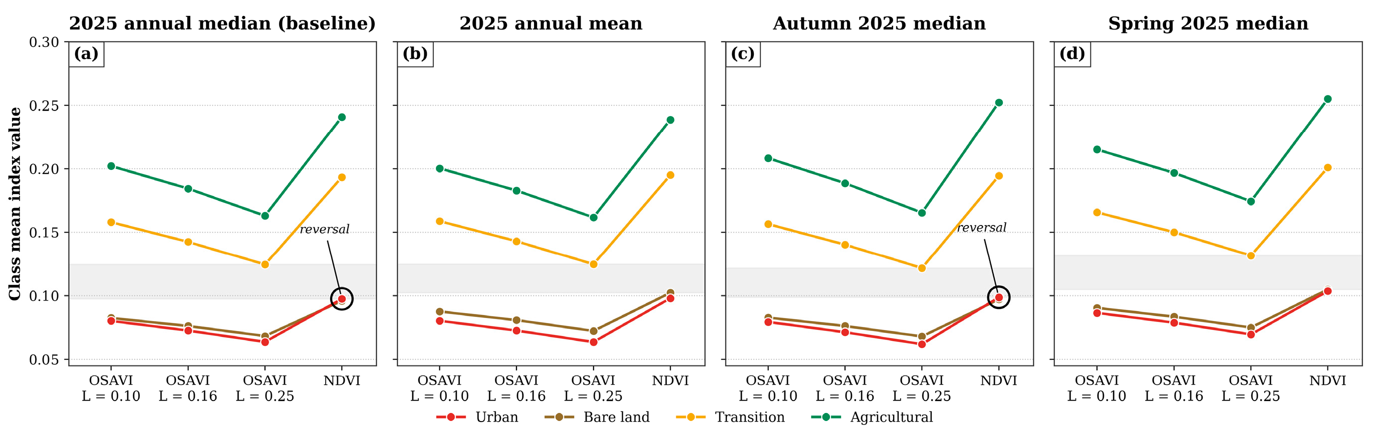
Figure A2 compares the Getis–Ord Gi* classification of the annual mean nocturnal LST at the native 1 km resolution under per-cell z-score thresholds (a) with the Benjamini–Hochberg FDR-corrected classification (b). The central urban hot spot persists under FDR control (23.0% of the 864 valid cells remain significant hot spots and 25.8% significant cold spots), confirming that the cluster identified in Section 4.4 is significant under conservative multiple-testing control and is not contingent on the resampling of the thermal field, since this analysis is performed entirely at the native 1 km resolution.
Figure A2.
Getis–Ord Gi* classification of the annual mean nocturnal LST at the native 1 km resolution: per-cell z-score thresholds (a) and Benjamini–Hochberg FDR-corrected significance (b), classifying hot and cold spots at the 90%, 95%, and 99% confidence levels (FDR panel at q = 0.10, 0.05, and 0.01).
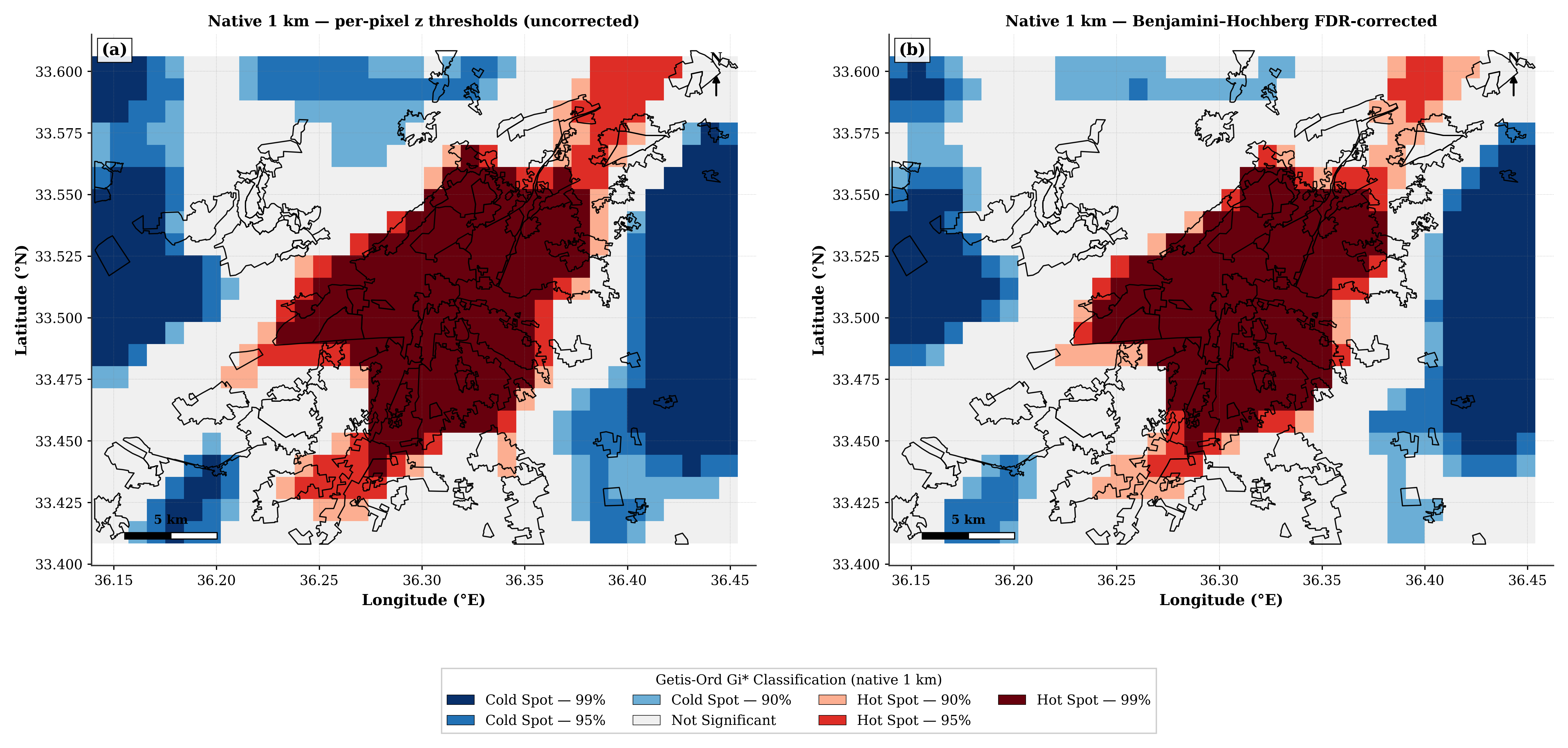
References
- United Nations. World Urbanization Prospects: The 2018 Revision; United Nations Department of Economic and Social Affairs, Population Division: New York, NY, USA, 2018; Available online: https://population.un.org/wup/assets/WUP2018-Highlights.pdf (accessed on 4 May 2026).
- Oke, T.R. The energetic basis of the urban heat island. Q. J. R. Meteorol. Soc. 1982, 108, 1–24. [Google Scholar] [CrossRef] [Scilit]
- Heaviside, C.; Vardoulakis, S.; Cai, X.-M. Attribution of mortality to the urban heat island during heatwaves in the West Midlands, UK. Environ. Health 2016, 15, S27. [Google Scholar] [CrossRef] [Scilit] [PubMed]
- Santamouris, M. Recent progress on urban overheating and heat island research: Integrated assessment of the energy, environmental, vulnerability and health impact, synergies with the global climate change. Energy Build. 2020, 207, 109482. [Google Scholar] [CrossRef] [Scilit]
- Sarrat, C.; Lemonsu, A.; Masson, V.; Guedalia, D. Impact of urban heat island on regional atmospheric pollution. Atmos. Environ. 2006, 40, 1743–1758. [Google Scholar] [CrossRef] [Scilit]
- Lelieveld, J.; Proestos, Y.; Hadjinicolaou, P.; Tanarhte, M.; Tyrlis, E.; Zittis, G. Strongly increasing heat extremes in the Middle East and North Africa (MENA) in the 21st century. Clim. Change 2016, 137, 245–260. [Google Scholar] [CrossRef] [Scilit]
- Voogt, J.A.; Oke, T.R. Thermal remote sensing of urban climates. Remote Sens. Environ. 2003, 86, 370–384. [Google Scholar] [CrossRef] [Scilit]
- Arnfield, A.J. Two decades of urban climate research: A review of turbulence, exchanges of energy and water, and the urban heat island. Int. J. Climatol. 2003, 23, 1–26. [Google Scholar] [CrossRef] [Scilit]
- Peng, S.; Piao, S.; Ciais, P.; Friedlingstein, P.; Ottle, C.; Bréon, F.-M.; Nan, H.; Zhou, L.; Myneni, R.B. Surface urban heat island across 419 global big cities. Environ. Sci. Technol. 2012, 46, 696–703. [Google Scholar] [CrossRef] [Scilit] [PubMed]
- Imhoff, M.L.; Zhang, P.; Wolfe, R.E.; Bounoua, L. Remote sensing of the urban heat island effect across biomes in the continental USA. Remote Sens. Environ. 2010, 114, 504–513. [Google Scholar] [CrossRef] [Scilit]
- Clinton, N.; Gong, P. MODIS detected surface urban heat islands and sinks: Global locations and controls. Remote Sens. Environ. 2013, 134, 294–304. [Google Scholar] [CrossRef] [Scilit]
- Santamouris, M. Regulating the damaged thermostat of the cities—Status, impacts and mitigation challenges. Energy Build. 2015, 91, 43–56. [Google Scholar] [CrossRef] [Scilit]
- Lazzarini, M.; Marpu, P.R.; Ghedira, H. Temperature-land cover interactions: The inversion of urban heat island phenomenon in desert city areas. Remote Sens. Environ. 2013, 130, 136–152. [Google Scholar] [CrossRef] [Scilit]
- Rasul, A.; Balzter, H.; Smith, C. Diurnal and seasonal variation of surface urban cool and heat islands in the semi-arid city of Erbil, Iraq. Climate 2016, 4, 42. [Google Scholar] [CrossRef] [Scilit]
- Zhou, D.; Zhao, S.; Liu, S.; Zhang, L.; Zhu, C. Surface urban heat island in China’s 32 major cities: Spatial patterns and drivers. Remote Sens. Environ. 2014, 152, 51–61. [Google Scholar] [CrossRef] [Scilit]
- Kim, Y.; Yoo, C.; Im, J. Nighttime satellite land surface temperature for urban applications: Achievements, challenges, and future prospects. GISci. Remote Sens. 2025, 62, 2527990. [Google Scholar] [CrossRef] [Scilit]
- Zhao, L.; Oppenheimer, M.; Zhu, Q.; Baldwin, J.W.; Ebi, K.L.; Bou-Zeid, E.; Guan, K.; Liu, X. Interactions between urban heat islands and heat waves. Environ. Res. Lett. 2018, 13, 034003. [Google Scholar] [CrossRef] [Scilit]
- Schwarz, N.; Lautenbach, S.; Seppelt, R. Exploring indicators for quantifying surface urban heat islands of European cities with MODIS land surface temperatures. Remote Sens. Environ. 2011, 115, 3175–3186. [Google Scholar] [CrossRef] [Scilit]
- Zhao, L.; Lee, X.; Smith, R.B.; Oleson, K. Strong contributions of local background climate to urban heat islands. Nature 2014, 511, 216–219. [Google Scholar] [CrossRef] [Scilit] [PubMed]
- Asgarian, A.; Amiri, B.J.; Sakieh, Y. Assessing the effect of green cover spatial patterns on urban land surface temperature using landscape metrics approach. Urban Ecosyst. 2015, 18, 209–222. [Google Scholar] [CrossRef] [Scilit]
- Weng, Q. Thermal infrared remote sensing for urban climate and environmental studies: Methods, applications, and trends. ISPRS J. Photogramm. Remote Sens. 2009, 64, 335–344. [Google Scholar] [CrossRef] [Scilit]
- Wan, Z. New refinements and validation of the MODIS land-surface temperature/emissivity products. Remote Sens. Environ. 2008, 112, 59–74. [Google Scholar] [CrossRef] [Scilit]
- Wan, Z.; Zhang, Y.; Zhang, Q.; Li, Z.L. Quality assessment and validation of the MODIS global land surface temperature. Int. J. Remote Sens. 2004, 25, 261–274. [Google Scholar] [CrossRef] [Scilit]
- World Meteorological Organization. Damascus, Syrian Arab Republic—Climatological Information. World Weather Information Service. Available online: https://worldweather.wmo.int/ar/city.html?cityId=213 (accessed on 12 June 2026).
- Azhdari, A.; Soltani, A.; Alidadi, M. Urban morphology and landscape structure effect on land surface temperature: Evidence from Shiraz, a semi-arid city. Sustain. Cities Soc. 2018, 41, 853–864. [Google Scholar] [CrossRef] [Scilit]
- Stewart, I.D.; Krayenhoff, E.S.; Voogt, J.A.; Lachapelle, J.A.; Allen, M.A.; Broadbent, A.M. Time evolution of the surface urban heat island. Earth’s Future 2021, 9, e2021EF002178. [Google Scholar] [CrossRef] [Scilit]
- Zhou, B.; Rybski, D.; Kropp, J.P. The role of city size and urban form in the surface urban heat island. Sci. Rep. 2017, 7, 4791. [Google Scholar] [CrossRef] [Scilit] [PubMed]
- Guo, A.; Yang, J.; Sun, W.; Xiao, X.; Cecilia, J.X.; Jin, C.; Li, X. Impact of urban morphology and landscape characteristics on spatiotemporal heterogeneity of land surface temperature. Sustain. Cities Soc. 2020, 63, 102443. [Google Scholar] [CrossRef] [Scilit]
- Gorelick, N.; Hancher, M.; Dixon, M.; Ilyushchenko, S.; Thau, D.; Moore, R. Google Earth Engine: Planetary-scale geospatial analysis for everyone. Remote Sens. Environ. 2017, 202, 18–27. [Google Scholar] [CrossRef] [Scilit]
- Rondeaux, G.; Steven, M.; Baret, F. Optimization of soil-adjusted vegetation indices. Remote Sens. Environ. 1996, 55, 95–107. [Google Scholar] [CrossRef] [Scilit]
- Olofsson, P.; Foody, G.M.; Herold, M.; Stehman, S.V.; Woodcock, C.E.; Wulder, M.A. Good practices for estimating area and assessing accuracy of land change. Remote Sens. Environ. 2014, 148, 42–57. [Google Scholar] [CrossRef] [Scilit]
- Pontius, R.G., Jr.; Millones, M. Death to Kappa: Birth of quantity disagreement and allocation disagreement for accuracy assessment. Int. J. Remote Sens. 2011, 32, 4407–4429. [Google Scholar] [CrossRef] [Scilit]
- Jensen, J.R. Introductory Digital Image Processing: A Remote Sensing Perspective, 4th ed.; Pearson: London, UK, 2016. [Google Scholar]
- Ord, J.K.; Getis, A. Local spatial autocorrelation statistics: Distributional issues and an application. Geogr. Anal. 1995, 27, 286–306. [Google Scholar] [CrossRef] [Scilit]
- Guerri, G.; Crisci, A.; Congedo, L.; Munafò, M.; Morabito, M. A functional seasonal thermal hot-spot classification: Focus on industrial sites. Sci. Total. Environ. 2022, 806, 151383. [Google Scholar] [CrossRef] [Scilit] [PubMed]
- Ghanghermeh, A.; Roshan, G.; Asadi, K.; Attia, S. Spatiotemporal Analysis of Urban Heat Islands and Vegetation Cover Using Emerging Hotspot Analysis in a Humid Subtropical Climate. Atmosphere 2024, 15, 161. [Google Scholar] [CrossRef] [Scilit]
- Benjamini, Y.; Hochberg, Y. Controlling the false discovery rate: A practical and powerful approach to multiple testing. J. R. Stat. Soc. Ser. B Methodol. 1995, 57, 289–300. [Google Scholar] [CrossRef] [Scilit]
- Dale, M.R.T.; Fortin, M.-J. Spatial Analysis: A Guide for Ecologists, 2nd ed.; Cambridge University Press: Cambridge, UK, 2014. [Google Scholar]
- Guha, S.; Govil, H.; Dey, A.; Gill, N. Analytical study of land surface temperature with NDVI and NDBI using Landsat 8 OLI and TIRS data in Florence and Naples city, Italy. Eur. J. Remote Sens. 2018, 51, 667–678. [Google Scholar] [CrossRef] [Scilit]
- Athukorala, D.; Murayama, Y. Urban heat island formation in Greater Cairo: Spatio-temporal analysis of daytime and nighttime land surface temperatures along the urban-rural gradient. Remote Sens. 2021, 13, 1396. [Google Scholar] [CrossRef] [Scilit]
- Peel, M.C.; Finlayson, B.L.; McMahon, T.A. Updated world map of the Koppen-Geiger climate classification. Hydrol. Earth Syst. Sci. 2007, 11, 1633–1644. [Google Scholar] [CrossRef] [Scilit]
- Giorgi, F.; Lionello, P. Climate change projections for the Mediterranean region. Glob. Planet. Change 2008, 63, 90–104. [Google Scholar] [CrossRef] [Scilit]
- Hajat, S.; Proestos, Y.; Araya-Lopez, J.-L.; Economou, T.; Lelieveld, J. Current and future trends in heat-related mortality in the MENA region: A health impact assessment with bias-adjusted statistically downscaled CMIP6 (SSP-based) data and Bayesian inference. Lancet Planet Health 2023, 7, e282–e290. [Google Scholar] [CrossRef] [Scilit] [PubMed]
- World Bank. Syria: World Bank US$146 Million Grant to Improve Electricity Supply and Support Sector Development. Press Release. 25 June 2025. Available online: https://www.worldbank.org/en/news/press-release/2025/06/25/syria-world-bank-us-146-million-grant-to-improve-electricity-supply-and-support-sector-development (accessed on 27 August 2026).
- Weng, Q.; Lu, D.; Schubring, J. Estimation of land surface temperature-vegetation abundance relationship for urban heat island studies. Remote Sens. Environ. 2004, 89, 467–483. [Google Scholar] [CrossRef] [Scilit]
- Bowler, D.E.; Buyung-Ali, L.; Knight, T.M.; Pullin, A.S. Urban greening to cool towns and cities: A systematic review of the empirical evidence. Landsc. Urban Plan. 2010, 97, 147–155. [Google Scholar] [CrossRef] [Scilit]
- Ayek, A. Nocturnal Surface Urban Heat Island Dynamics in a Semi-Arid Mediterranean City: Evidence from Damascus. Zenodo 2026. [Google Scholar] [CrossRef]
- World Bank. Syria Physical Damage and Reconstruction Assessment 2011–2024; World Bank: Washington, DC, USA, 2025; Available online: https://documents.worldbank.org/en/publication/documents-reports/documentdetail/099102025095540101 (accessed on 27 August 2026).
- UNITAR-UNOSAT. Syria: Eastern Ghouta Area/Damascus Governorat—Imagery Analysis: 23 February 2018. United Nations Institute for Training and Research, Operational Satellite Applications Programme. 2018. Available online: https://reliefweb.int/map/syrian-arab-republic/syria-eastern-ghouta-area-damascus-governorate-imagery-analysis-23-february (accessed on 27 August 2026).
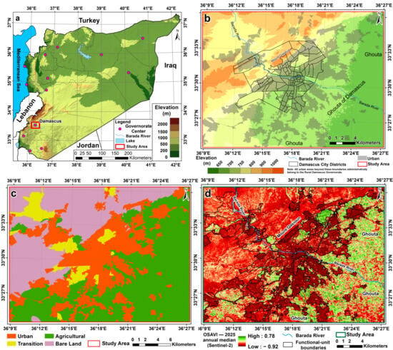
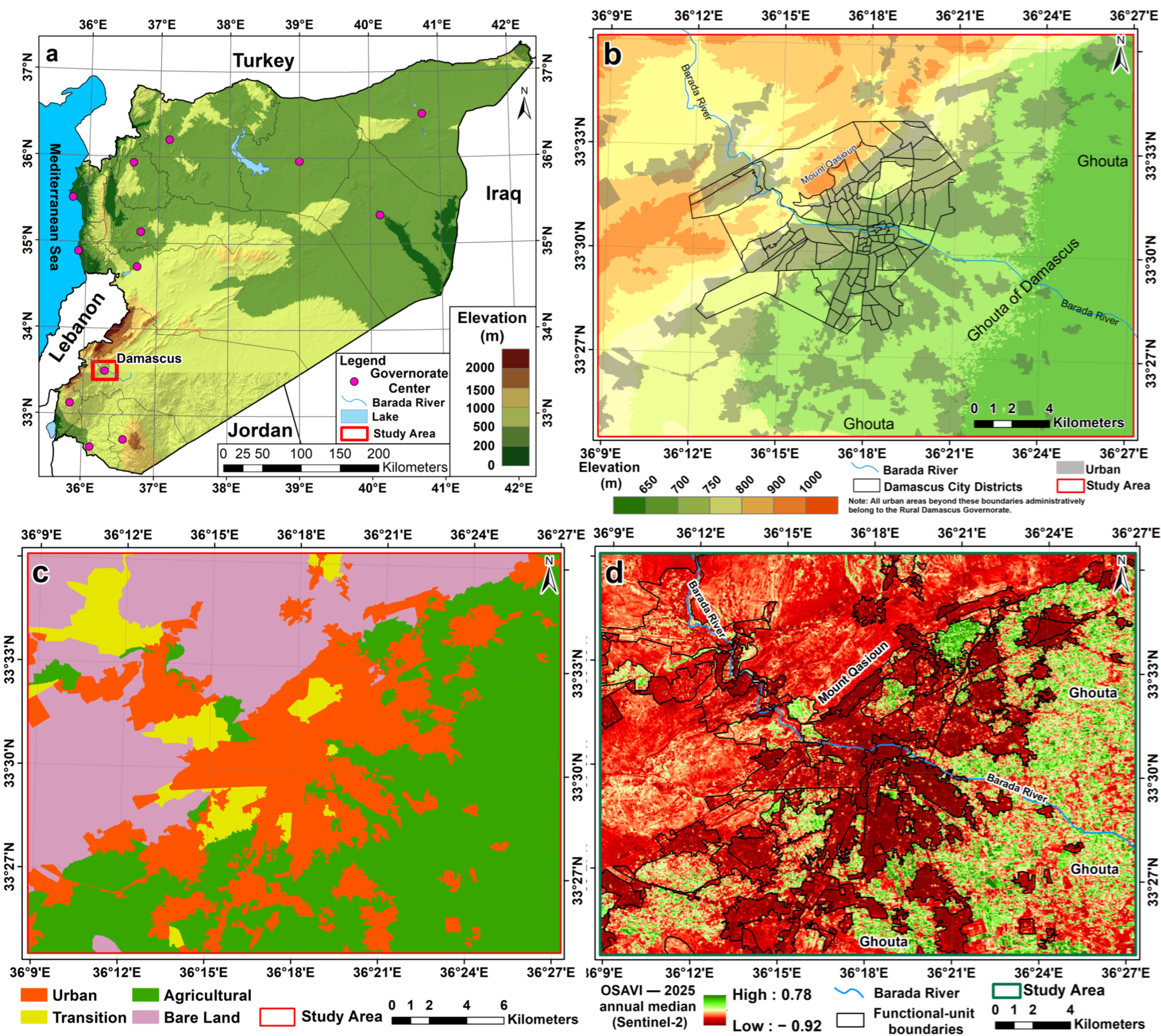
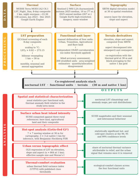
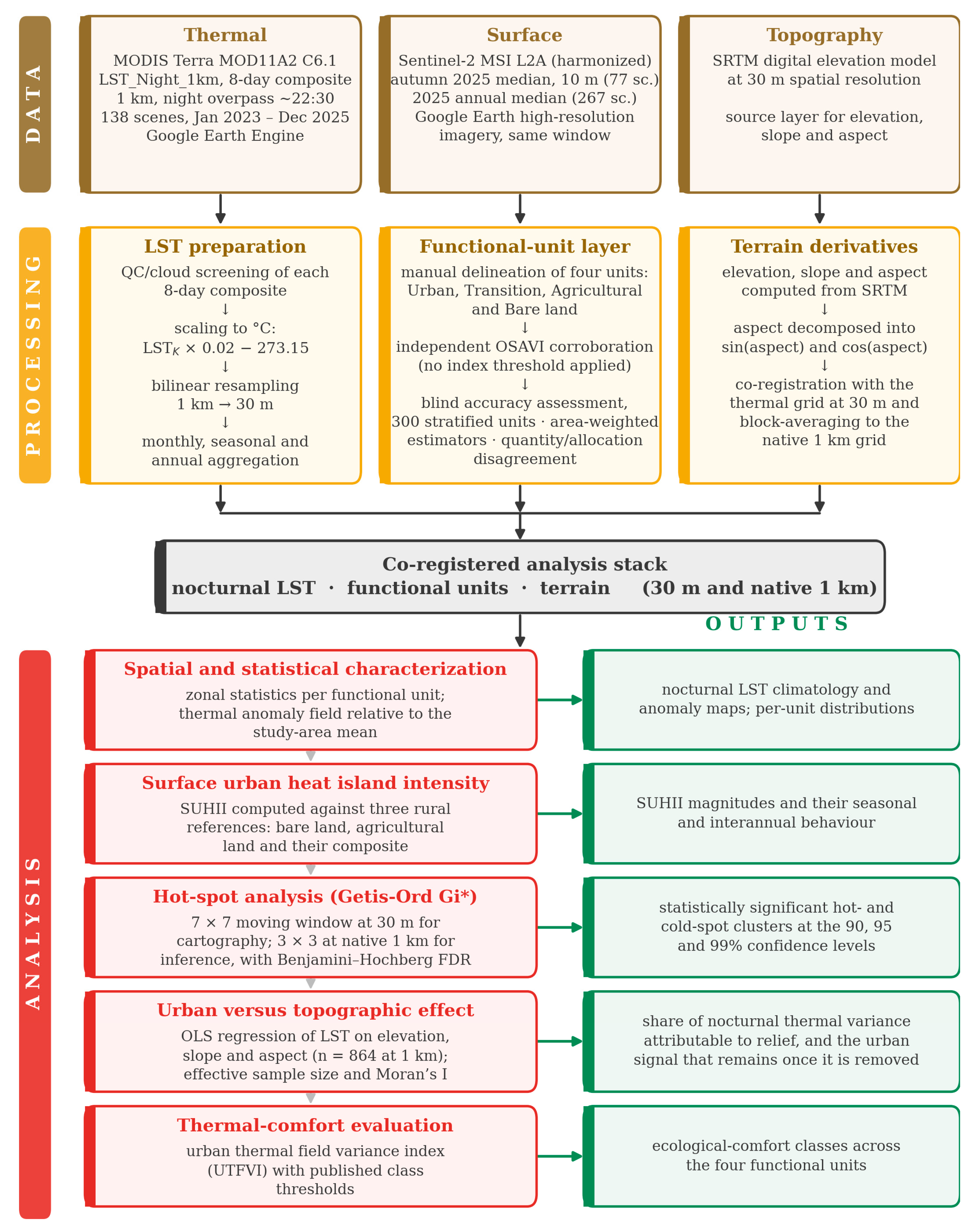
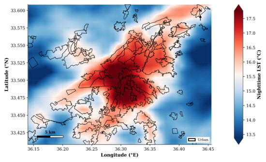
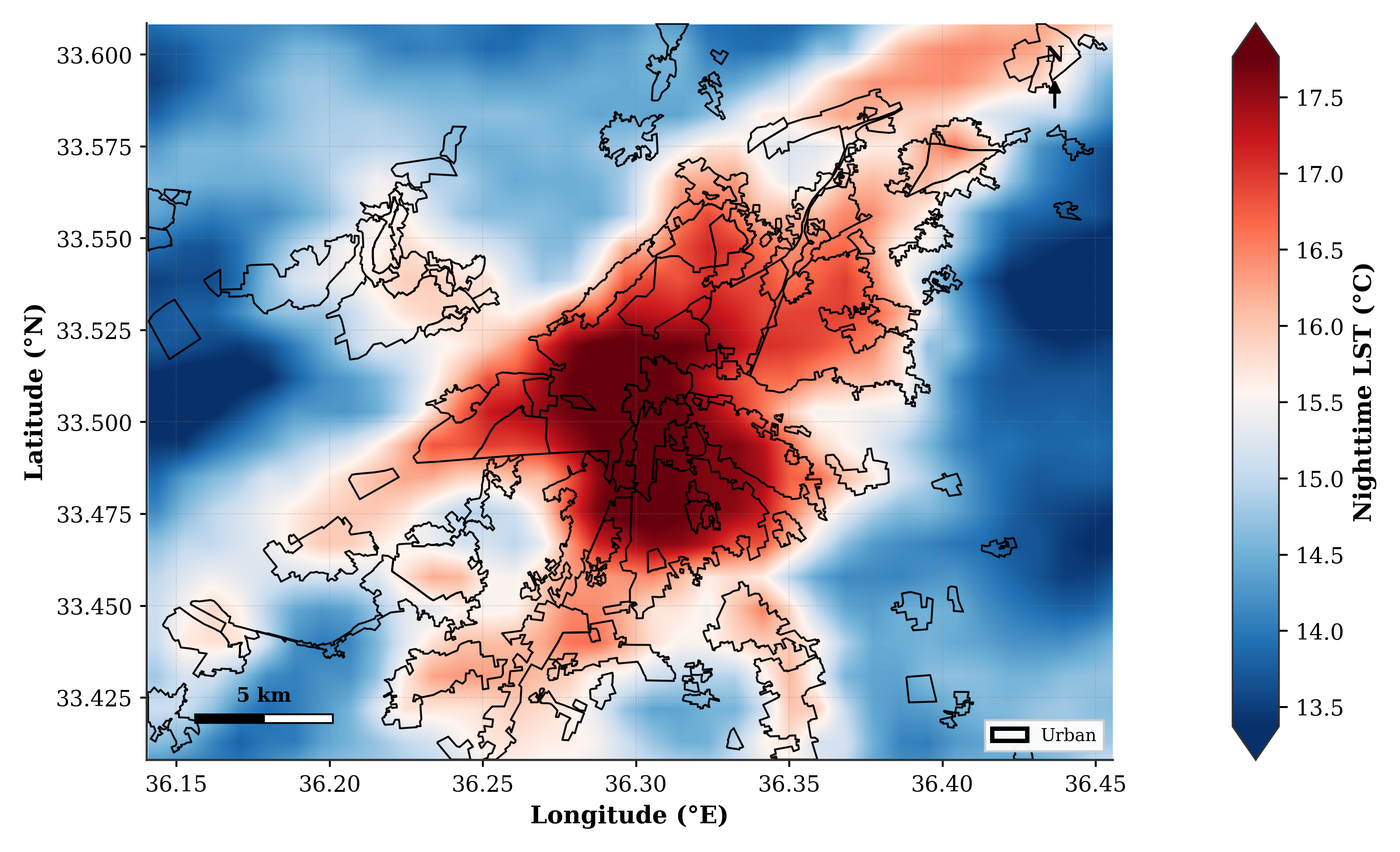
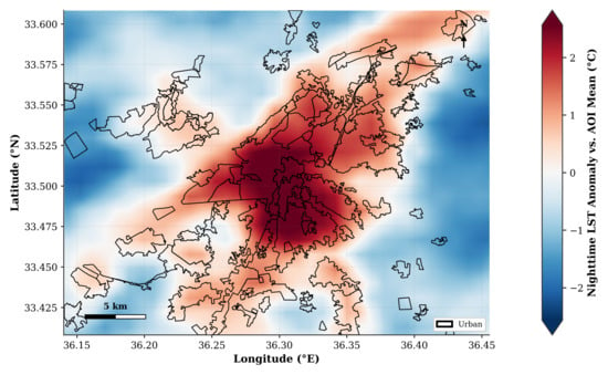
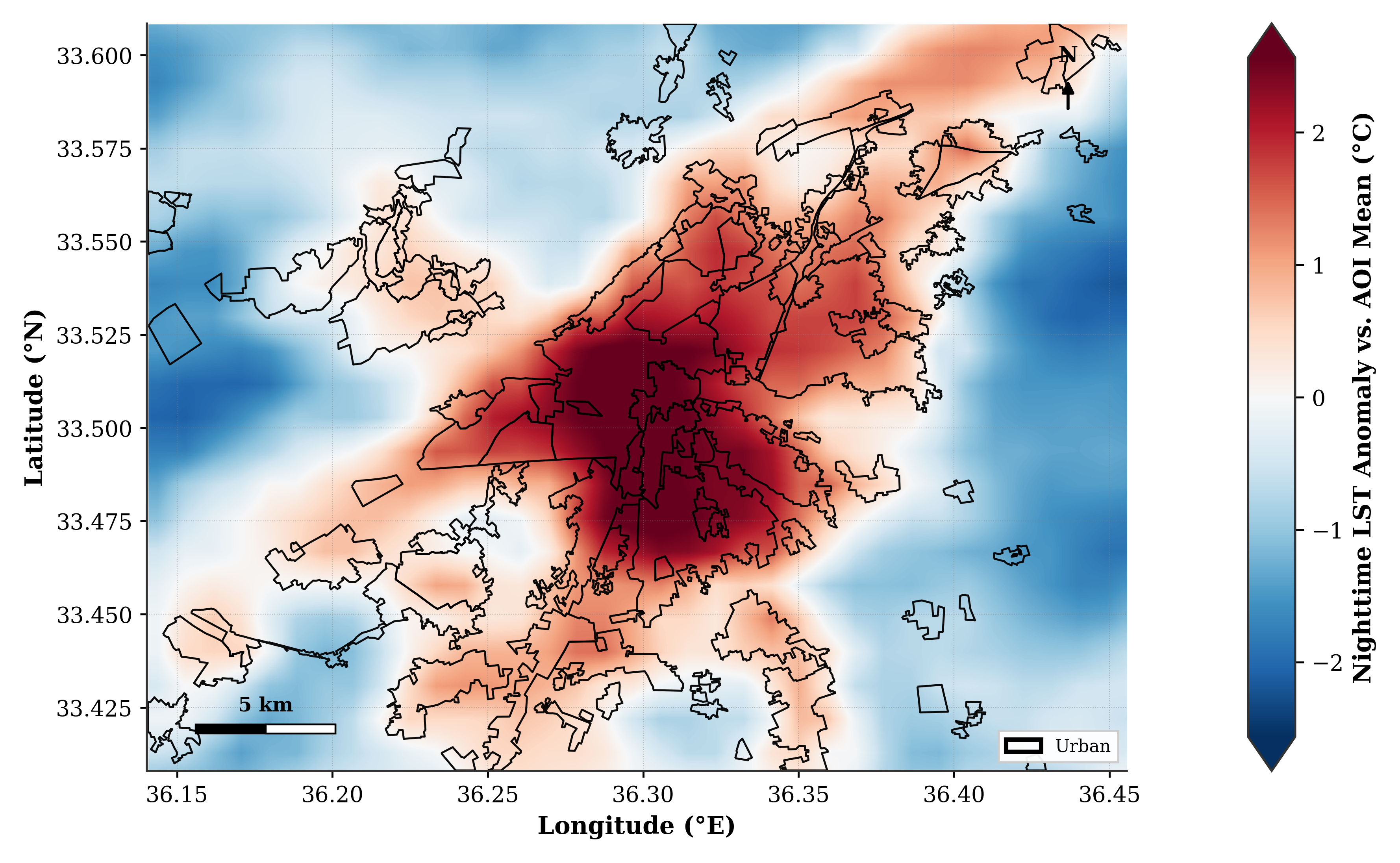
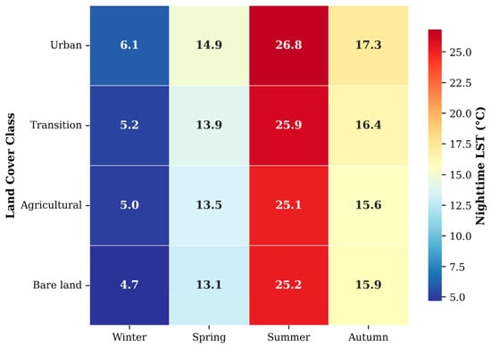
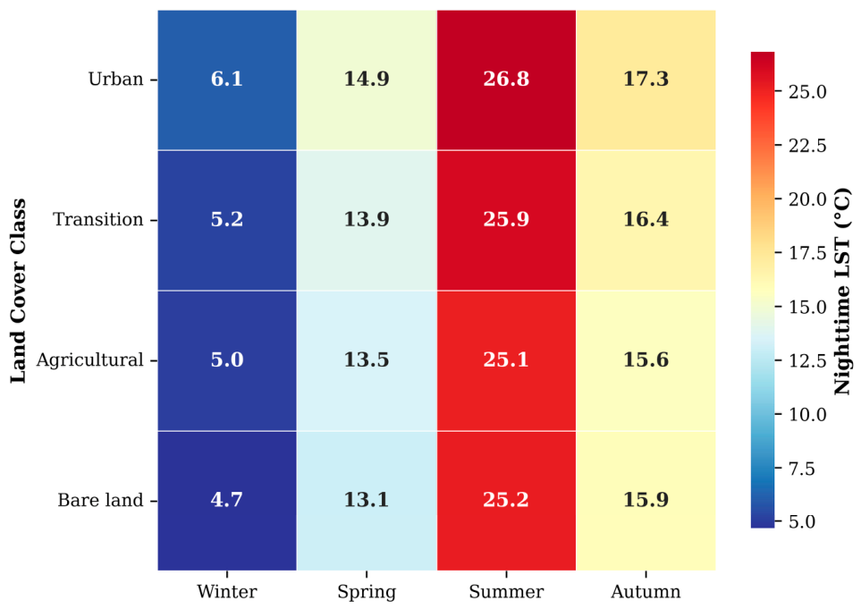
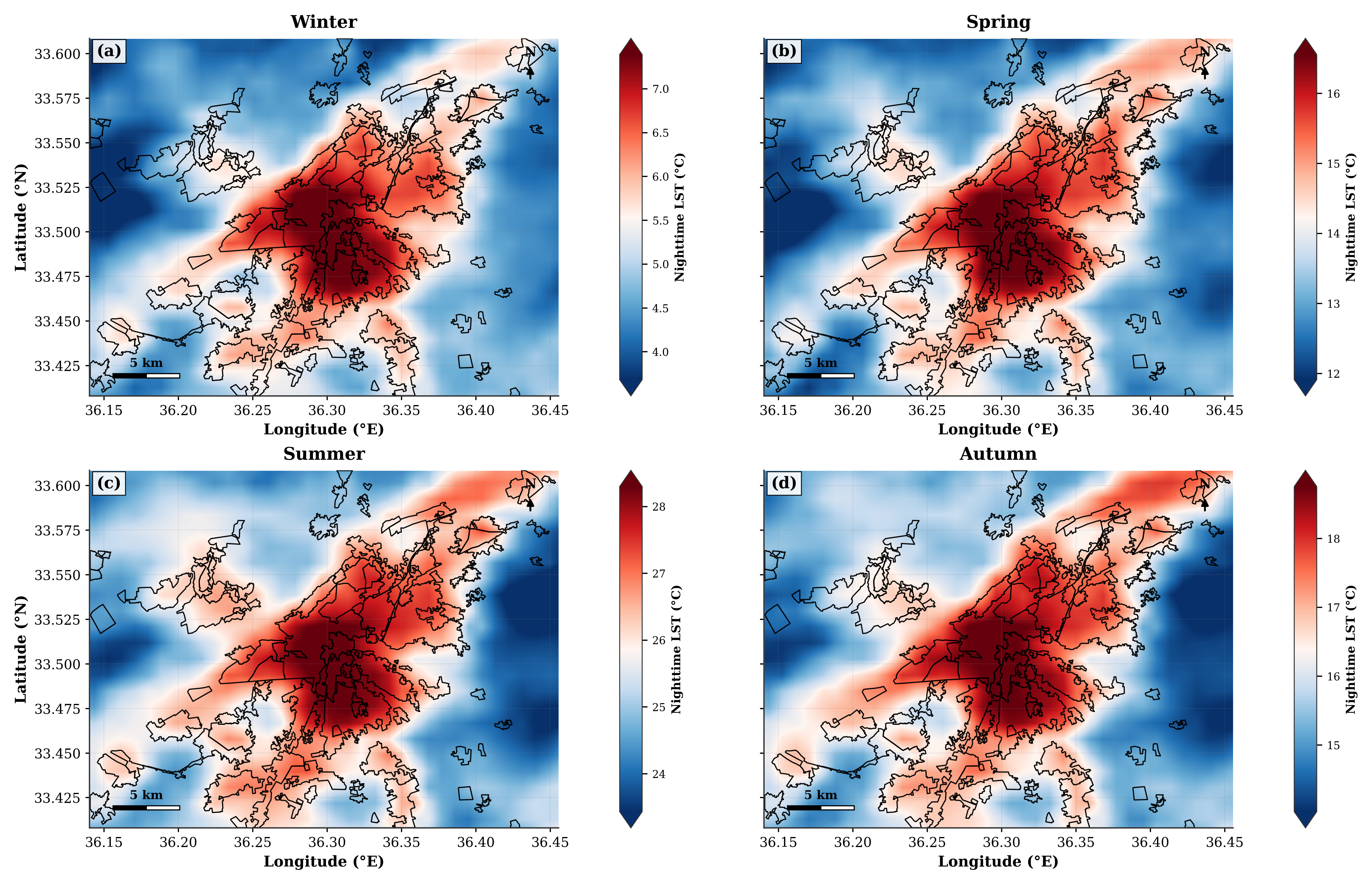
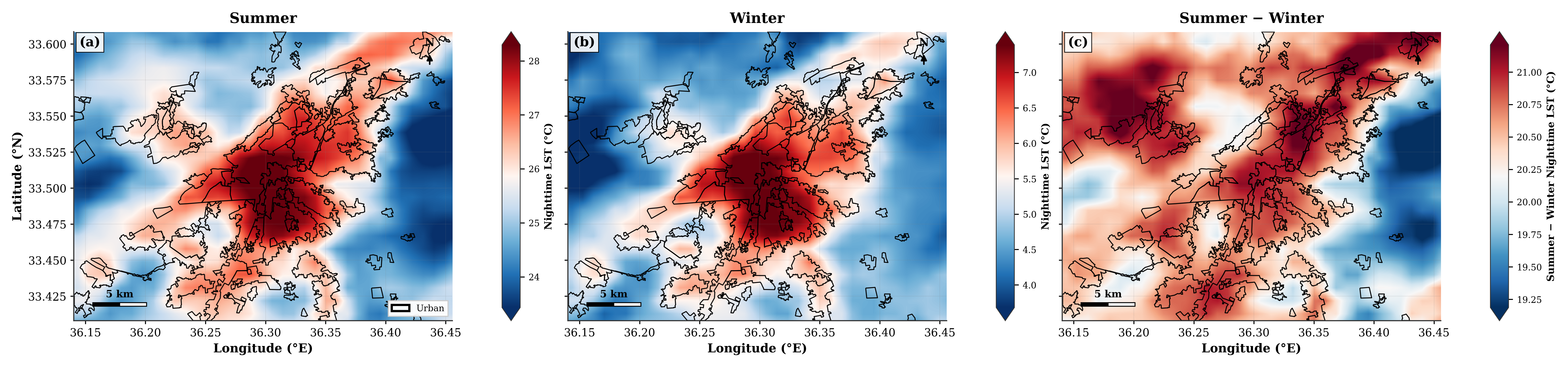
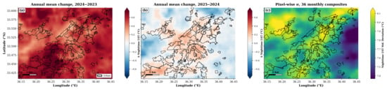
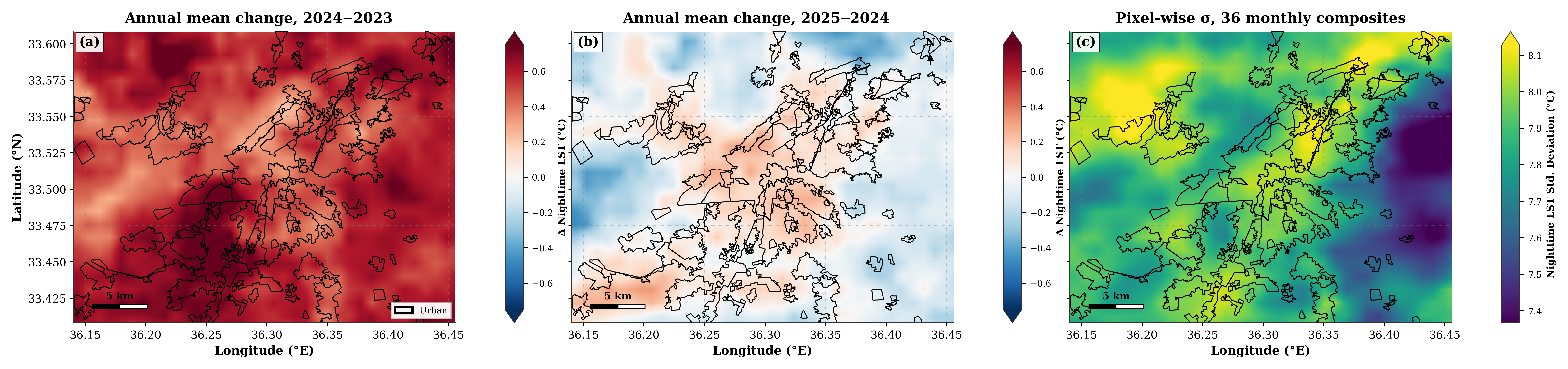
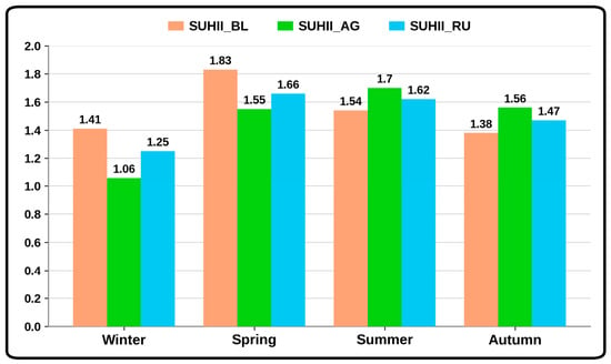
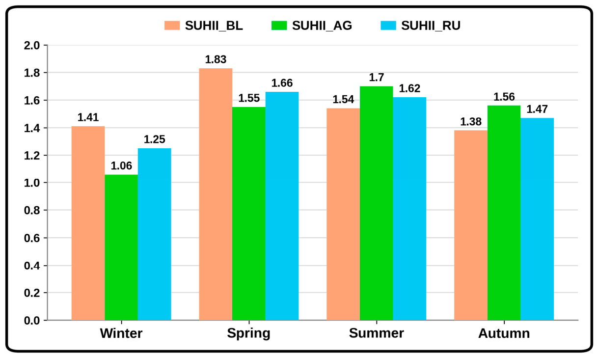
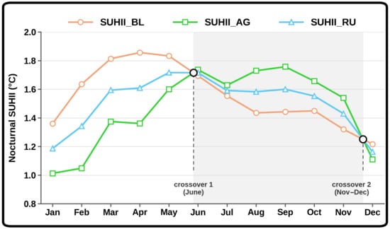
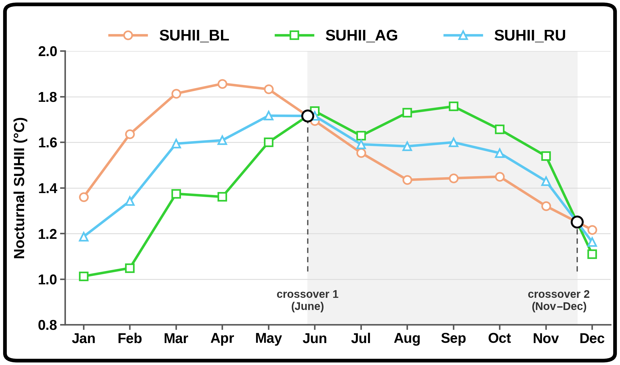
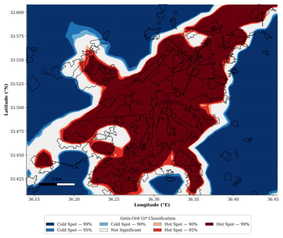
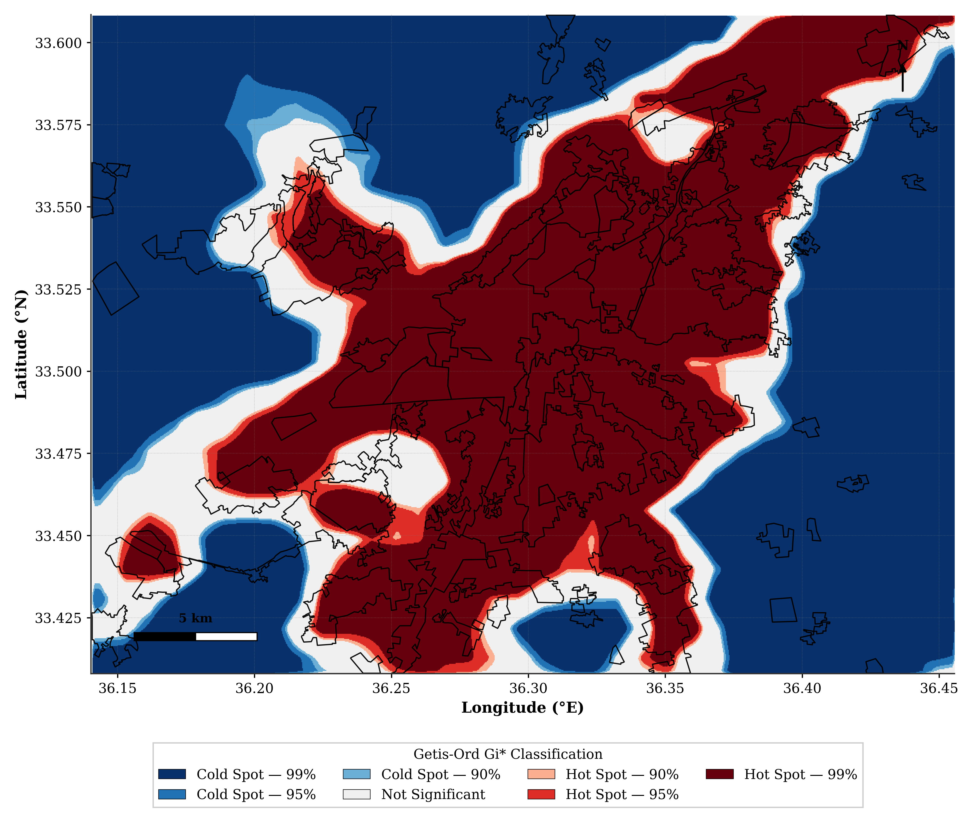
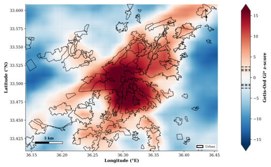
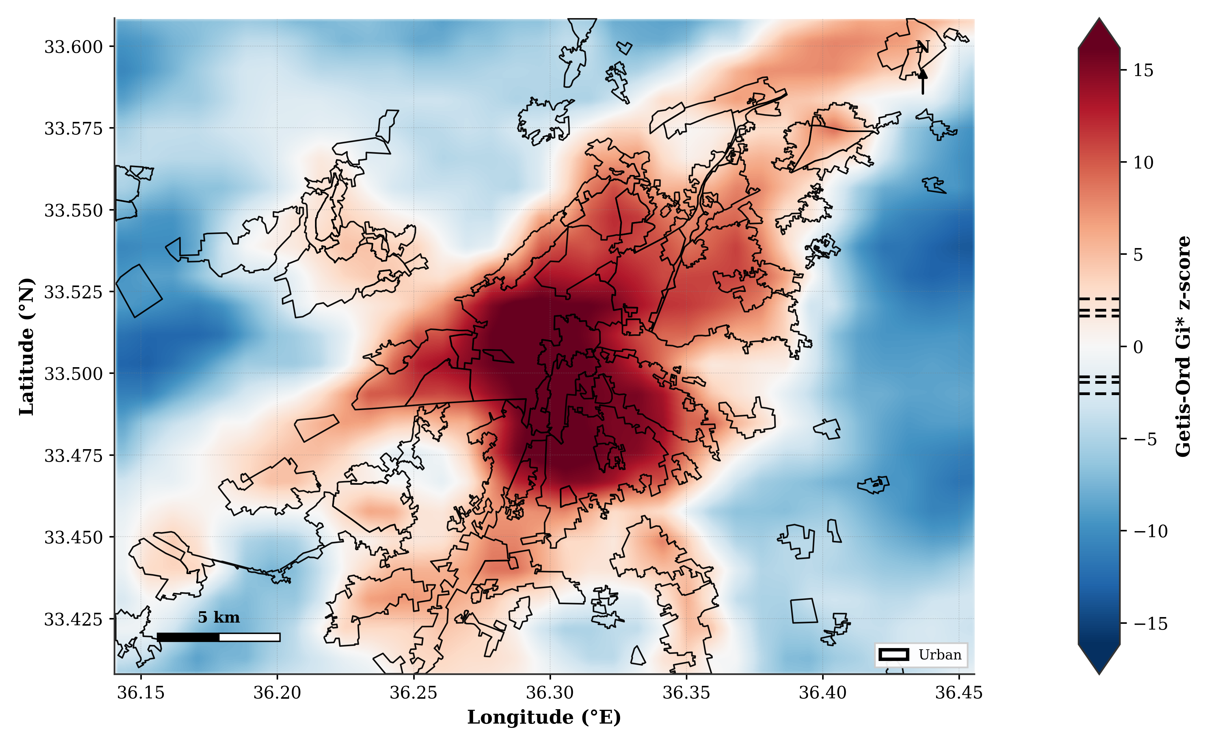
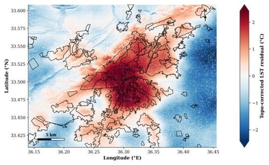
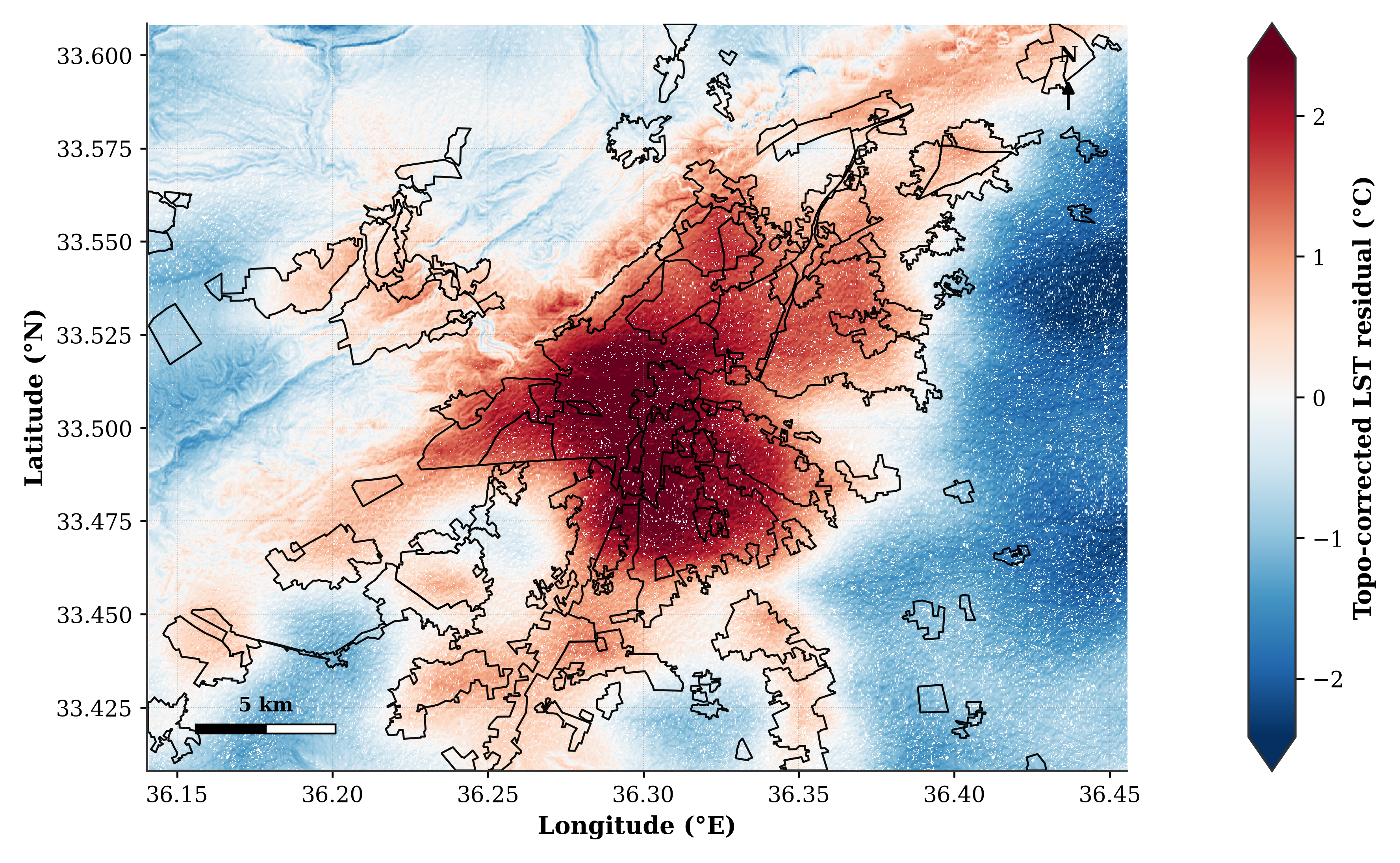
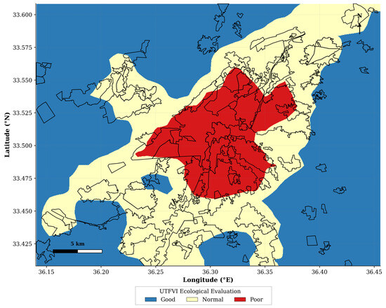
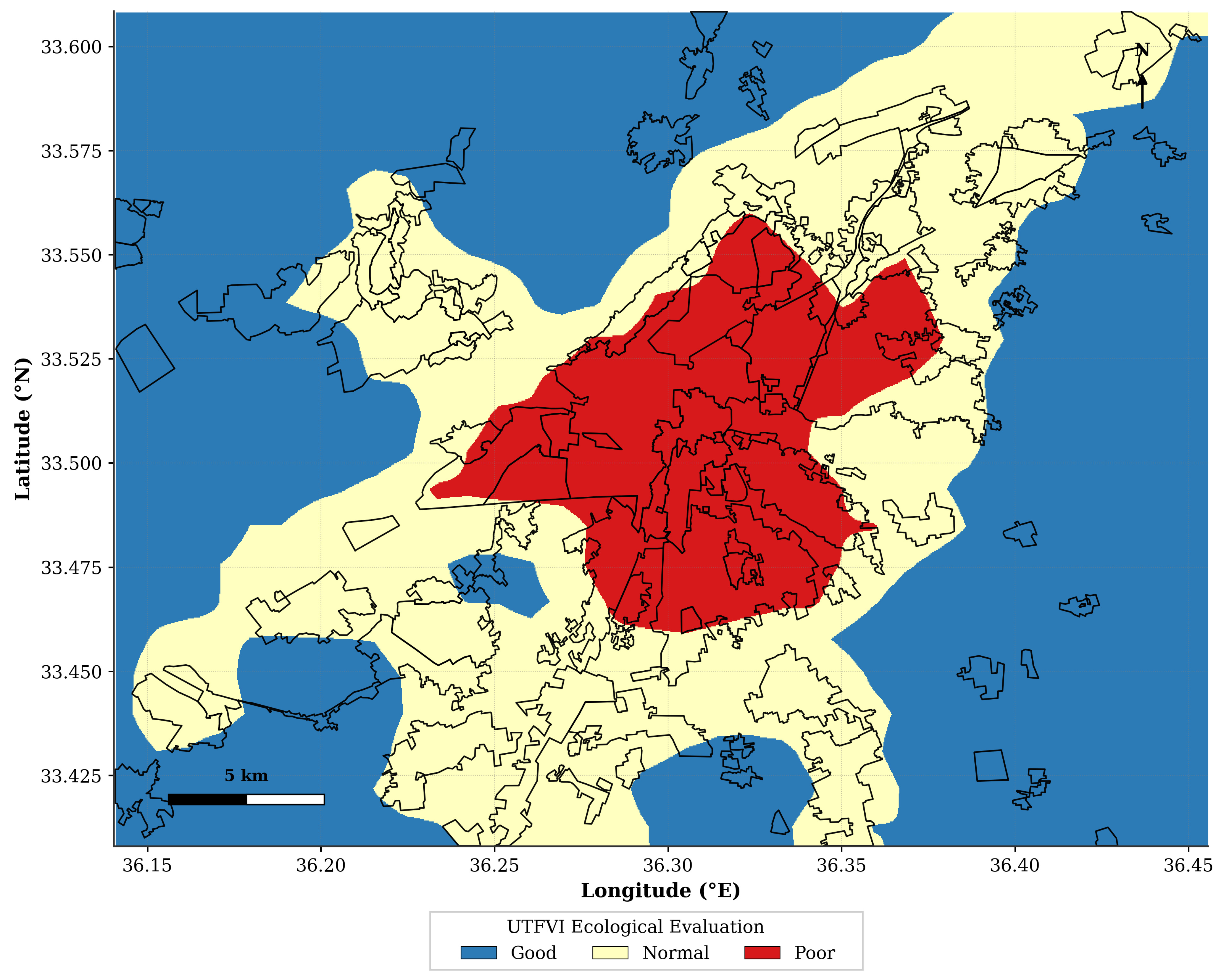
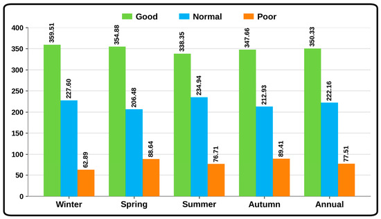
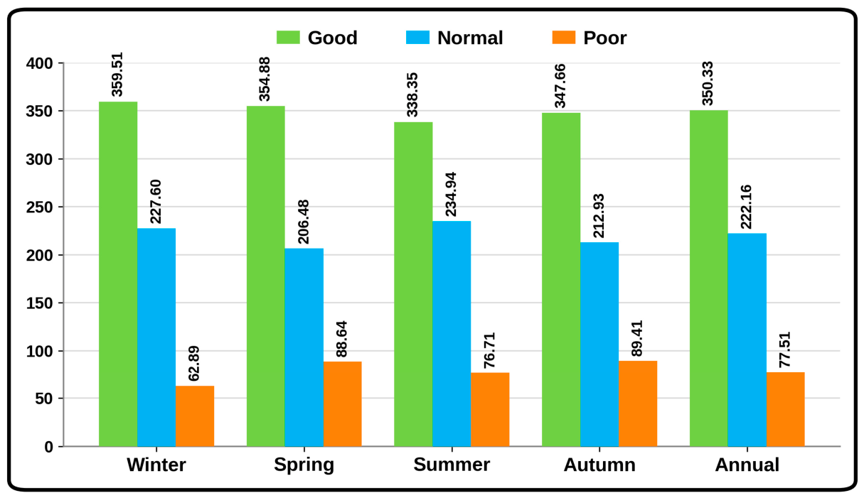
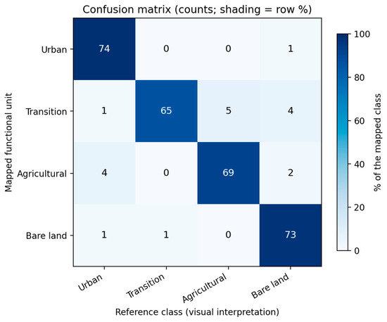

Disclaimer/Publisher’s Note: The statements, opinions and data contained in all publications are solely those of the individual author(s) and contributor(s) and not of MDPI and/or the editor(s). MDPI and/or the editor(s) disclaim responsibility for any injury to people or property resulting from any ideas, methods, instructions or products referred to in the content. |
© 2026 by the authors. Licensee MDPI, Basel, Switzerland. This article is an open access article distributed under the terms and conditions of the Creative Commons Attribution (CC BY) license.