


Abstract
Real estate market risk has long been a core policy concern for governments worldwide, as risks across the land, real estate, and financial markets are inherently deeply coupled. Accurate measurement and early warning of systemic risks in the land–real estate–financial market system constitute a critical prerequisite for forestalling major economic fluctuations. In the era of big data, the proliferation of high-frequency, large-scale, and multi-dimensional market data poses formidable challenges to conventional risk assessment frameworks. Grounded in the perspective of interlinkages among the land, real estate, and financial markets, this paper employs the BEKK-GARCH model to construct a time-varying composite risk index and further incorporates the CNN-LSTM machine learning model to provide early warning of coupled risks in the land–real estate–financial market system. The empirical results demonstrate that the constructed composite risk index exhibits strong validity and high sensitivity, and the findings remain robust under stochastic scenarios. Compared with other benchmark early-warning models, the CNN-LSTM model delivers superior overall early-warning performance. The findings of this study carry significant practical implications for dynamically monitoring and providing early warning of real estate market risks in the context of big data, curbing cross-market risk contagion, and safeguarding the sustainable and sound development of the land–real estate–finance nexus.
1. Introduction
1.1. Background
In recent years, beset by economic shocks and inventory overhang, regional real estate markets have exhibited pronounced divergence, with housing prices in many cities continuing to experience heightened volatility. Moreover, risk factors across the land market, real estate market, and financial sector frequently overlap, making the evolution and resolution of diversified, cross-market risks a key area of ongoing surveillance for macroprudential authorities worldwide. Establishing a scientific and objective early-warning mechanism to identify real estate risks earlier and more accurately is of considerable practical significance for stabilizing the housing market, curbing cross-market risk transmission within the land–real estate–finance nexus, preventing and defusing risks in key sectors, and promoting the sustainable and sound development of the land and real estate markets.
The marginal contributions of this paper are as follows: (1) In response to the heterogeneous, high-frequency, and high-dimensional characteristics of contemporary big data for real estate monitoring, a dual-layer early-warning indicator system is constructed. (2) From the perspective of three-dimensional interconnectedness among the land, real estate, and financial markets, the BEKK-GARCH model is employed to synthesize a time-varying composite real estate risk index, thereby identifying cross-market risk contagion. (3) A hybrid deep learning model integrating convolutional neural networks and long short-term memory networks (CNN-LSTM) is developed to deliver graded early warning of coupled risks within the land–real estate–finance system. The lightweight CNN-LSTM model constructed herein is well suited to small- and medium-sized datasets, and its multilayer regularization design comprehensively suppresses overfitting, ensuring higher early-warning accuracy and strong model stability.
1.2. Literature Review
Since the 2008 global subprime mortgage crisis, the intertwining relationships among the land market, real estate market, and financial market have drawn increasing scholarly attention. The global subprime crisis revealed that relying solely on microprudential regulation and ex post risk resolution is insufficient to effectively forestall the accumulation and outbreak of systemic risks [1]. This recognition has spurred both academia and policy circles to shift their research focus toward the construction of ex ante early-warning mechanisms. Prior studies typically treat land as the cost side of housing supply, the real estate market as an intermediary between the household sector and the banking system, and the financial market as a source of external shocks and risk pricing, thereby examining the linkages between land and housing prices or the risk transmission between the real estate market and the financial market [2,3,4,5,6,7]. The existing literature demonstrates that rising land prices weaken housing supply responsiveness and amplify house price spikes [8]. Conditional on the relaxation of borrowing constraints, an increase in house prices generates a strong incentive for leveraged households to invest more in residential property [9]. The integration of financial intermediation into the real economy affects the real estate sector’s output, value added, and pricing [10].
However, relatively few studies to date have integrated the land market, real estate market, and financial market into a unified framework to examine cross-market risk interconnectedness. Some research suggests that land financialization and housing financialization are not mutually independent processes. Housing assetization expands the demand for land, while land financialization sustains real estate market expansion through accelerated land supply and the capitalization of land prices [11]. In the context of China, excessive local government reliance on land financialization may exacerbate local debt risks [12,13]. Findings from several other studies further indicate that the impact of land financialization on the real estate market exhibits a threshold effect. At lower levels of land financialization, the gentrification effect is limited or even negative; this pattern is driven by urban revitalization initiatives and gradual property value appreciation in the early stages of urban development. However, once land financialization exceeds a certain threshold, intensified investment and speculative activity substantially fuel property price growth [14]. Rising residential land prices transmit upward to housing prices and exacerbate credit misallocation [15].
Early frameworks for real estate risk evaluation and forecasting include nonlinear decomposition methods, Bayesian stochastic frontier models, Markov regime-switching models, and DSGE models [16,17,18,19]. When conventional modeling approaches are applied, the selection and quantity of explanatory variables directly shape the model’s early-warning performance [20]. In recent years, driven by advances in computing power and algorithmic innovation in the big data era, researchers have introduced machine learning methods into real estate risk early-warning research—including BP neural networks, PSO-SVM, random forests, and artificial neural networks (ANNs) [21,22,23,24]. Scholars have explored the application pathways of tree-based machine learning techniques in the context of derivative pricing and confirmed that fully trained gradient boosting models can deliver rapid price predictions for new underlying assets [25]. LSTM models dominate financial market forecasting across stocks, foreign exchange, bonds, and cryptocurrencies, while CNN-LSTM architectures are increasingly widely adopted for their ability to capture complex spatiotemporal dependencies [26,27,28]. These methods offer distinct strengths in data fault tolerance, nonlinear fitting capacity, and generalization performance.
Nevertheless, several limitations remain in the extant literature. First, most existing real estate risk indices are constructed via weighted aggregation and principal component analysis. Such fixed-weight approaches struggle to accurately capture the time-varying nature of systemic real estate risk, and prior studies have generally paid insufficient attention to the cross-market contagion mechanisms of real estate risk. Second, there is scant research in the extant literature on an early-warning framework that simultaneously integrates the three-dimensional risks of land, real estate, and finance and exhibits strong nonlinear mapping capacity. Third, most empirical studies rely on annual or quarterly data, for which their low frequency falls short of the timeliness requirements for real-time risk monitoring.
To adapt to the current complex data environment characterized by nonlinearity, high frequency, and high dimensionality, this paper improves traditional real estate risk evaluation methods from multiple dimensions: the construction of cross-market indicators covering land, real estate, and finance, the BEKK-GARCH-based indicator synthesis approach, and the design of the CNN-LSTM risk early-warning model so as to generate risk early-warning reports with stronger timeliness and stability.
The remainder of this paper is organized as follows: Section 2 describes the selection of early-warning indicators and the synthesis of the cross-market composite risk index; Section 3 elaborates on the algorithmic principles, simulation results, and performance evaluation of the CNN-LSTM early-warning model; Section 4 concludes with policy recommendations and directions for future research.
2. Materials and Methods
2.1. Two-Tier Indicator System Framework
Systemic risk measurement for the real estate market must not be limited to the isolated monitoring of risks within a single market. Instead, it should integrate multiple cross-sectoral risk sub-indicators, covering the allocation of real estate market factors, land market supply dynamics, and financing coordination among financial institutions.
This paper constructs a three-dimensional foundational indicator pool covering the land, real estate, and finance sectors. For each of the three dimensions, multiple representative second-tier indicators are selected to form a two-tier indicator system for measuring systemic risk in the real estate market (see Table 1 for details). All indicators in Table 1 are calculated as year-on-year growth rates, which serve two purposes: first, to better capture underlying market trends, and second, to eliminate data fluctuations driven by seasonal effects. The rationale for selecting core indicators in each subdomain is elaborated below:
Table 1.
Two-tier indicator system for three-dimensional land–real estate–finance coupled risk.
- (1)
- Rationale for Land Market Risk Indicators: Excessively high year-on-year growth in transacted land area and total land transaction value can directly drive up corporate leverage and financing costs. A high average land premium rate erodes developers’ profit margins, and developers may pass costs to homebuyers by raising selling prices, thereby exerting upward pressure on future housing prices. The average land auction failure rate reflects market sentiment and competition vitality: a rising failure rate is usually associated with pessimistic expectations for future market conditions, insufficient land acquisition funds, and constrained financing channels, among other factors [29,30]. Second-tier indicators in the land domain are optimal at moderate levels; the larger their absolute values, the greater the stress on the land market.
- (2)
- Rationale for Supply–Demand Risk Indicators in the Real Estate Market: The supply–demand nexus forms the core mechanism for value realization in the real estate sector. Year-on-year growth rates of newly commenced floor area and sold floor area capture the operational efficiency of the real estate market across the full construction-to-sales cycle. Both incremental supply and unsold inventory levels affect the long-term stability of the real estate market [31]. A year-on-year rise in unsold floor area signals sluggish market sales, which further intensifies funding pressure on property developers. As house price fluctuations are tied to changes in economic fundamentals and even the formation of market-wide bubbles [32], house price dynamics serve as a core indicator for assessing real estate market risks [33,34,35]. Substantial period-on-period volatility in new and second-hand home prices indicates a degree of supply–demand imbalance in the market. These indicators are optimal at moderate levels; the larger their absolute values, the higher the risk level in the real estate market.
- (3)
- Rationale for Financial Institution Real Estate Exposure Risk Indicators. Real estate market risks can spill over to the financial market through balance sheet channels in both the corporate and household sectors. First, real estate development loans rely heavily on indirect bank financing. When developers face sluggish sales cash flow, credit default risks emerge [36] and transmit to the financial sector via the balance sheet channel. Second, falling house prices erode collateral values, raising mortgage default risks among highly leveraged households, particularly those with subprime mortgages [37], which directly undermines the soundness of financial institutions’ balance sheets. The larger the absolute values of second-tier indicators in the real estate finance domain, the greater the instability in the financial market exposed to real estate risks.
2.2. Data Sources
This paper uses China’s national-level monthly data covering the period from January 2012 to December 20252, all sourced from the Wind database. Unlike prior studies that directly aggregate all indicators into a single composite index, this paper accounts for cross-market risk correlations and spillover effects across the land, real estate, and financial markets and constructs the index based on a two-tier indicator framework. Specifically, disaggregated indicators in each of the three markets are first aggregated into corresponding sub-risk indices. The BEKK-GARCH time-varying correlation coefficient matrix is then applied to further construct the composite real estate risk index, which better captures cross-market risk interconnections.
2.3. Research Methods for Composite Risk Index Construction
2.3.1. Indicator Normalization
To address the issue of inconsistent data scales, this paper adopts the empirical cumulative distribution function (ECDF) method for dimensionless normalization of the raw data. The ECDF transformation does not require the sample to follow a normal distribution; it preserves the intrinsic characteristics of the original series to the maximum extent and reduces the sensitivity of transformed data to extreme values.
For a given indicator variable, let all its observations be denoted as x = (x1, x2, …, xn), where n is the total number of observations. For negative-direction indicators, values are first negated before ECDF transformation. The ECDF transformation for each observation xt is defined as
where 1(·) is the indicator function: it takes a value of 1 if the condition is satisfied, and 0 otherwise.
2.3.2. Sub-Index Synthesis Based on CRITIC–Entropy Weight Method
The preprocessed dimensionless data are aggregated into sub-indices for each submarket using the CRITIC–entropy weight method. This combined weighting approach is adopted for the following reason: While the CRITIC method accounts for the variability and conflict among indicators and captures their nonlinear relationships, it does not take the dispersion degree of indicators as a core weighting criterion. The entropy weight method, by contrast, determines indicator weights primarily based on their dispersion level. The combination of the CRITIC and entropy weight methods thus produces more objective indicator weights.
Let there be T time-series observations and n evaluation indicators, with the raw data denoted as . Here, T denotes all time points in the sample, and n denotes the number of indicators within each submarket. The CRITIC method is applied to calculate weights across indicators; the information content of the j-th indicator is computed as follows:
where denote the standard deviation and the mean of the j-th indicator, respectively, and is the correlation coefficient between the k-th and the j-th indicator. The weight of the j-th indicator is given by
The entropy weight method is applied to calculate the weights, with the probability of occurrence of the j-th indicator for the i-th evaluation object (time point) computed as
The information entropy of the j-th indicator is calculated as
The weight of the j-th indicator is
In summary, the weight of the j-th indicator is. Assuming that the two weighting methods are of equal importance, β = 0.53.
2.3.3. Synthesis of the Risk Index Based on the Time-Varying Correlation Coefficient Matrix
Based on the sub-indices , and synthesized via the CRITIC–entropy weight method described above, let denote the vector matrix comprising the three sub-indices , and let w be the corresponding weight vector of the three sub-indices. Following the approach adopted in prior studies, the weights among the sub-indices are determined according to the cumulative impulse response values of the sub-indices to the month-on-month growth rate of China’s industrial production index within a VAR model, which better captures time-varying characteristics [38,39]. The calculation formula is as follows:
where ⊙ denotes the Hadamard product. The composite real estate risk index in this paper can be defined as
where is the time-varying correlation coefficient matrix, which captures the interconnections among the three market segments examined in this study. The strength of the correlations among the three risk sub-indices is a key determinant of the level of systemic risk in the real estate market. When high correlations exist among the sub-segments, the overall risk in the real estate sector becomes compounded; conversely, when correlations among the sub-segments are low, the overall risk reflected in the real estate sector does not accumulate rapidly. The formula for is given by
where denotes the correlation coefficient between sub-index i and sub-index j at time t. To obtain the above time-varying correlation coefficient matrix , it is necessary to first derive the time-varying covariance matrix using the BEKK-GARCH model. After is normalized to the interval [0, 1], it is adjusted by subtracting its theoretical median of 0.5 (which is identical to its mean value) to obtain [38,39,40]. A trivariate diagonal BEKK-GARCH model is then constructed as follows:
where is a lower triangular matrix, and matrices A and B are parameter matrices. This model can more accurately capture the time-varying correlations among the sub-indices. To address the issue of high parameter dimensionality, we adopt the diagonal BEKK specification, in which matrices A and B are restricted to being diagonal matrices. is the covariance matrix, as shown in Equation (11) below:
where denotes the conditional variance of sub-index i when i = j and the conditional covariance between sub-index i and sub-index j when i ≠ j at time t. From the equation above, it follows that
2.4. Research Methodology for the Risk Early-Warning Model
2.4.1. Overall Architecture of the CNN-LSTM Model
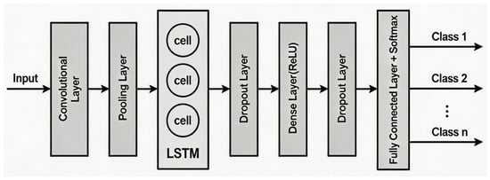
The CNN-LSTM model constructed in this paper adopts an overall lightweight design philosophy, controlling the base capacity of the model through small-size convolutional kernels and low-dimensional hidden units. By regulating the scale of convolutional kernels and the dimensionality of hidden layers to constrain the overall parameter capacity, it reduces the risk of overfitting on the premise of ensuring effective feature extraction and adapts to the requirements of classification tasks in small-sample scenarios.
The model as a whole consists of three cascaded modules: a local feature extraction module, a temporal dependency modeling module, and a classification output module.
The local feature extraction module is composed of a single-layer 1D convolutional layer (Conv1D) and a single-layer 1D max-pooling layer (MaxPooling1D). The convolutional layer is configured with 8 parallel convolutional kernels with a temporal kernel size of 3 and adopts the Rectified Linear Unit (ReLU) as the activation function to capture local correlation patterns of adjacent features in the input sequence. The subsequent max-pooling layer performs downsampling with a pooling window of 2. By retaining the extreme value features of local regions, it improves the model’s robustness against local perturbations.
The temporal dependency modeling module adopts a single-layer long short-term memory (LSTM) network structure, with the number of hidden units set to 8. It only outputs the hidden state vector at the final time step, which can be directly connected to the subsequent fully connected classification module without additional flattening operations. To constrain the magnitude of weight parameters and suppress overfitting to training noise, L2 norm regularization is applied to this layer, with the regularization penalty coefficient set to 0.001.
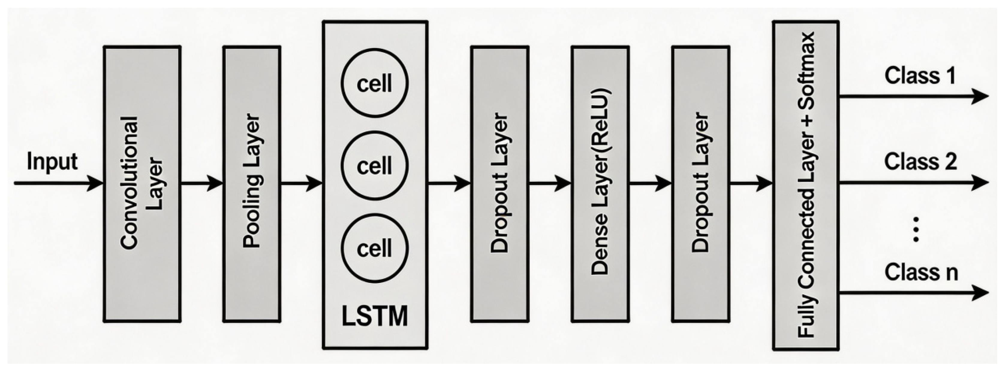
The classification output module is formed by cascading dropout layers and a fully connected network. To further improve the generalization performance of the model, dropout layers are added after the LSTM layer and the fully connected hidden layer, respectively, with neuron dropout rates set to 0.6 and 0.5 in sequence. By randomly deactivating part of the neurons during the training phase, it breaks the co-adaptation among features and prevents the model from making classification decisions that rely on a small number of local features. The fully connected network comprises two layers: The hidden layer has 16 neurons, adopts the ReLU activation function, and is simultaneously imposed with L2 norm regularization with a coefficient of 0.001; the number of neurons in the output layer automatically matches the actual total number of classes in the dataset. The Softmax activation function is used to map the outputs into a normalized class probability distribution, with the sum of all class probabilities equal to 1. Finally, class determination for the multi-class classification task is realized via the argmax of the probability distribution (Figure 1).
Figure 1.
Schematic diagram of the CNN-LSTM neural network architecture.
2.4.2. Training Strategy and Callback Mechanisms for Dynamic Regulation
In terms of data input and basic training configuration, the two-dimensional tabular data is reshaped into a three-dimensional tensor format, which conforms to the standard input specification of Conv1D. The first dimension corresponds to the number of training samples. The batch size is set to 8, and the shape of the input tensor for a single batch is (8 × 13 × 1). The second dimension is the sequence dimension. In line with the structural characteristics of monthly data, this study takes the feature dimension as the sequence length. The information value of monthly data lies not only in the temporal evolution across months but also in the strong correlations among land, real estate, and financial indicators within a single month. Modeling feature columns as a sequence enables in-depth exploration of the ordered linkage patterns of multi-dimensional indicators within one month. The convolution kernel slides along the sequence dimension, covering three adjacent features at each step to extract local correlation features. The third dimension is the channel dimension. Since there is only one numerical value at each feature position, the number of input channels is 1. The number of convolution kernels is set to 8; after passing through this layer, the number of output channels increases from 1 (input) to 8, and each kernel independently learns a local feature combination pattern. The maximum number of training epochs is set to 80.
We adopt the Adaptive Moment Estimation (Adam) algorithm as the optimizer. Combining the momentum principle and an adaptive learning rate mechanism, it features fast convergence and strong parameter robustness. Sparse Categorical Crossentropy is selected as the loss function, which can directly process integer class labels without additional one-hot encoding. The core evaluation metric for model training is classification accuracy. To prevent data leakage, normalization, oversampling, class weighting, and all model tuning are conducted using only the training data after the train/test split.
To address the imbalanced class distribution of samples, the model employs a dual correction mechanism integrating data-level and algorithm-level strategies. At the data level, a simple random oversampling strategy is applied to replicate and augment minority class samples in the training set, increasing their proportion. At the algorithm level, loss weights for each class are calculated based on the “balanced” criterion. During backpropagation, higher loss contribution weights are assigned to minority class samples to guide the model to learn feature patterns of all classes in a balanced manner.
To ensure training stability and build a multi-level overfitting prevention system, three types of callback mechanisms are introduced to form a dynamic regulation framework during training:
First, the Model Checkpoint Mechanism: It takes validation accuracy as the monitoring metric and only retains the model weights corresponding to the highest validation accuracy, ensuring optimal generalization performance of the final output model.
Second, the Early Stopping Mechanism: It monitors validation loss with a patience value of 10 epochs. When validation loss fails to decrease for consecutive epochs, training is automatically terminated, and the weights with the lowest validation loss are restored to avoid redundant iterations and aggravated overfitting.
Third, the ReduceLROnPlateau Adaptive Learning Rate Decay Mechanism: It also monitors validation loss, with a patience of 5 epochs and a decay factor of 0.5. When validation loss shows no improvement for 5 consecutive epochs, the learning rate is halved, with a minimum learning rate floor of 1 × 10⁻⁵. By dynamically reducing the optimization step size, it facilitates fine parameter tuning during the convergence plateau, further improving model performance.
2.4.3. Selection of Evaluation Metrics for Model Early-Warning Performance
To evaluate the early-warning performance of the model, four metrics are adopted for comprehensive assessment: accuracy, precision, recall, and the comprehensive evaluation metric F1 score. Accuracy captures the overall prediction accuracy of the model across the entire dataset. Precision measures the accuracy of the model when predicting positive class samples. Recall reflects the model’s ability to correctly identify positive class samples. The F1 score integrates the model’s precision and recall performance, with a value ranging from 0 to 1; a value closer to 1 indicates better early-warning performance. The corresponding calculation formulas are presented as follows:
where TP denotes the number of samples that are actually positive and correctly predicted as positive; TN denotes the number of samples that are actually negative and correctly predicted as negative; FP denotes the number of samples that are actually negative but incorrectly predicted as positive; FN denotes the number of samples that are actually positive but incorrectly predicted as negative.
3. Results
3.1. Measurement Results of the Coupled Risk Index
3.1.1. Synthesis Result of the Submarket Risk Index
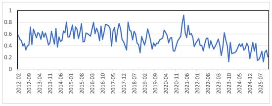
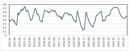
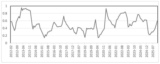
After normalizing each indicator in the risk indicator system table using the cumulative empirical distribution function method described above, the CRITIC–entropy weight method is applied to synthesize the sub-indices across indicators within each segment. This yields the land market risk sub-index , the real estate market risk sub-index , and the financial institution real estate exposure risk sub-index for China over the period from January 2012 to December 2025, as shown in Figure 2, Figure 3 and Figure 4.
Figure 2.
Trend of the land market risk sub-index.
Figure 3.
Trend of the real estate market risk sub-index.
Figure 4.
Trend of the real-estate-related financial market risk sub-index.
In 2013, housing prices in China rose, developers engaged in aggressive land acquisition, and substantial volumes of shadow banking and trust funds flowed into the real estate market, precipitating a rapid increase in the real estate risk index X2t and the real estate-related financial risk index X3t.
During the period from 2016 to 2017, housing prices in China’s first- and second-tier cities surged dramatically, land auctions repeatedly set new record prices, household leverage climbed, and developer debt expanded, with all three risk indices exhibiting a synchronized upward trend. After 2017, following the introduction of the “housing is for living in, not for speculation” policy, purchase restrictions, credit tightening, and sales restrictions were comprehensively intensified nationwide, and financing channels began to contract, leading to a decline in the real estate-related financial risk index X3t. From 2013 to 2019, the correlation between the real estate market risk index and the real estate-related financial market risk index strengthened, with their movements broadly coinciding.
In 2021, the formal implementation of the “Three Red Lines” policy severed the transmission of real estate market risks to the financial system, resulting in a gradual decoupling of the real estate risk index X2t and the real estate-related financial risk index X3t. The market expansion of highly leveraged, high-debt developers was constrained, and developers undertook almost no new speculative land acquisitions, leading to a downward trend in both the land market risk index X1t and the real estate-related financial market risk index X3t. After 2023, the commercial housing market experienced sluggish pricing, households adopted a wait-and-see stance, and the unsold inventory rate rose in certain regions, driving the real estate market risk index upward. From 2024 to 2025, national real estate policies shifted comprehensively toward “halting the decline and restoring stability,” with multiple measures implemented to enhance household housing affordability. This facilitated a gradual recovery in real estate market transaction volumes, eased destocking pressure, and resulted in the land and real estate market risk indices exhibiting low-level fluctuations.
3.1.2. Synthesis Result of the Coupled Risk Index
Given that risks inherent in the real estate market can be transmitted across the closely linked land market and real estate-related financial sectors, and that the intensity of risk contagion may amplify or attenuate over time, we follow established methodologies for determining risk weights in the prior literature [29,30,32] and construct a vector autoregressive (VAR) model with four variables: the land market risk sub-index, the real estate market risk sub-index, the financial institution real estate exposure risk sub-index, and the year-on-year monthly growth rate of China’s industrial production index4. This study calculates the cumulative impulse response of the month-on-month growth rate of industrial value-added over the subsequent 12 months to a one-unit positive shock from each of the three sub-indices and takes the absolute value of the cumulative response as a measure of the systemic impact intensity of each sub-index. Accordingly, the weights of the three sub-indices in Equation (7)—land market risk X1t, real estate market risk X2t, and financial institution real estate exposure risk X3t—are determined as 11.56%, 76.97%, and 11.47%, respectively. The real estate market accounts for the largest weight share, which aligns with the core characteristics of China’s real estate industry: It features a long industrial chain and extensive linkages with upstream and downstream sectors, and it functions as a pillar industry of the national economy. The marginal impact of fluctuations in real estate transactions and investment on the real economy is significantly greater than that of fluctuations in the land market and real-estate-related financial markets. Meanwhile, as a robustness check, we compute the composite risk index under an equal-weight scheme. The results indicate that the identification of risk states is not highly sensitive to the choice of weighting algorithm.5
In the BEKK-GARCH model, the diagonal matrices A and B are estimated as follows:
The diagonal elements of the estimated matrices A and B are all significantly positive at the 5% significance level. Matrix A indicates that the current-period volatility of each sub-market is driven by its own lagged idiosyncratic shocks. Among the three sub-markets, the real estate market records the largest coefficient of 0.4, implying that it is the most sensitive to abrupt shocks such as policy adjustments and macroeconomic events, and new external information is rapidly reflected in its contemporaneous volatility. Matrix B demonstrates that the volatility of each sub-market exhibits pronounced persistence. In particular, the GARCH coefficient of the housing-related financial sub-market reaches 0.967, representing the strongest volatility memory. The test confirms that the maximum eigenvalue of the matrix (A⊗A + B⊗B) is less than unity, indicating that the model satisfies the condition of covariance stationarity.
Table 2 reports the diagnostic test results for the standardized residuals. The ARCH-LM test results suggest that no significant remaining heteroskedasticity exists at the 5% significance level, indicating that the variance equation of the model has adequately captured the volatility clustering property of the original series. For the Ljung–Box test on level-standardized residuals, the real estate market and the housing-related financial market exhibit no significant autocorrelation at the 5% significance level, while the land market shows no significant autocorrelation in residuals at the 1% significance level. In general, the mean equation has effectively extracted the autocorrelation information embedded in the series. Furthermore, the Ljung–Box test on squared standardized residuals confirms that the squared standardized residual series also have no significant autocorrelation at the 5% significance level.
Table 2.
Results of ARCH-LM and Ljung–Box diagnostic tests.
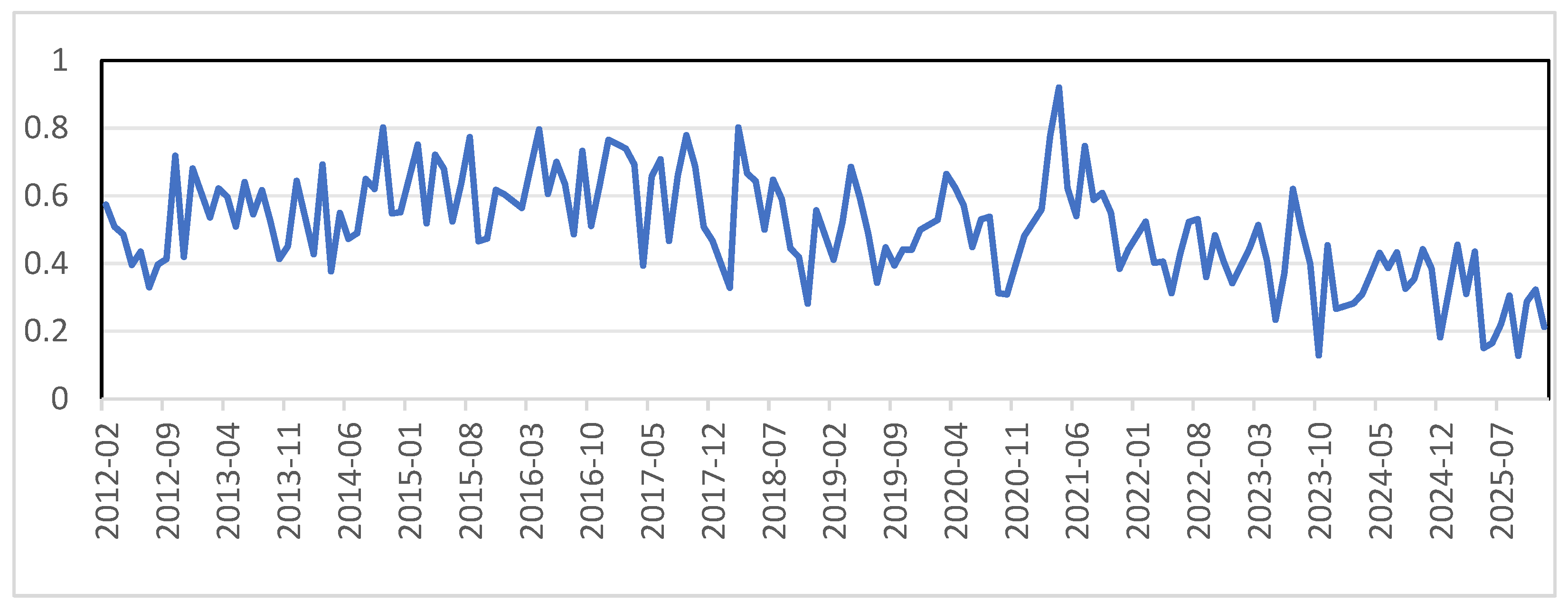
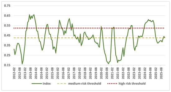
Subsequently, the BEKK-GARCH time-varying correlation coefficient matrix Ct is introduced, and Equations (8) and (9) are employed to synthesize the three sub-indices into the composite real estate risk index (see Figure 5 as shown in below).
Figure 5.
Coupled risk index of the land–real estate–real-estate-related finance nexus.
As shown in Figure 5, the maximum value of the systemic risk index for the land–real estate–real estate-related finance nexus is 0.6592, and the minimum value is 0.1622. Drawing on the analytical approaches adopted by scholars in the study of systemic financial risk, it is evident that shocks to the real estate market induced by major external events or sectoral regulatory policies alter the trajectory of the composite real estate risk index. The detailed analysis is as follows.
In 2012, two rounds of interest rate cuts by the People’s Bank of China injected ample liquidity into the market and enhanced the purchasing power of the rigid-demand segment. As sales recovered, developers’ willingness to replenish land inventories strengthened. In 2013, “land kings” emerged frequently and land premium rates surged, transmitting strong expectations of future housing price increases to the market, and the composite real estate risk index remained persistently elevated. In December 2013, the Central Economic Work Conference and the Central Urbanization Work Conference were held in succession. Against the backdrop of immense housing price appreciation pressure in 2013, first- and second-tier cities successively escalated regulatory tightening measures in December, putting a “brake” on the mounting real estate market risk. Consequently, the systemic real estate risk index declined gradually from 0.66 in December 2013 to 0.3 in September 2014. In March 2015, the People’s Bank of China, the Ministry of Housing and Urban-Rural Development, and the then China Banking Regulatory Commission jointly issued the “March 30 New Deal,” further lowering the home purchase threshold and supporting improvement-oriented demand. Although destocking pressure persisted in third- and fourth-tier cities, transactions in first- and second-tier cities recovered. During this phase, the composite real estate risk index fell gradually from 0.5618 in March 2015 to 0.2719 in December 2015. Following the announcement and implementation of the “Three Red Lines” policy targeting real estate development enterprises in 2021, the high-leverage operational risks of these enterprises were effectively brought under control. Superimposed on the sales downturn during the pandemic period, this directly triggered debt defaults among multiple developers, and unfinished and abandoned housing projects emerged in certain regions. Consequently, real estate market risks reverberated successively between enterprises and financial institutions. Market transaction volumes remained sluggish, housing prices stayed under sustained pressure, and the systemic risk index rose steeply from 0.2393 in March 2022, reaching a periodic high of 0.6097 in June 2024. Entering 2025, with the substantive disbursement of government special-purpose bond funds for land reserve acquisition and existing housing stock purchases, the narrowing of housing price declines in core cities, and the incremental demand generated by urban village redevelopment, the real estate market began to exhibit signs of bottoming out. The systemic real estate risk index shifted from oscillating at elevated levels into a downward channel, fluctuating around the 0.4 level throughout the year.
In summary, the fluctuation characteristics of the synthesized composite risk index curve largely align with the fundamentals of the real estate market and major regulatory policies, which, to a certain extent, corroborate the sensitivity and validity of the composite real estate risk index constructed in this paper.
3.1.3. Determination Results of Early-Warning Thresholds
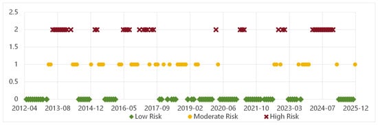
To circumvent the stochastic bias arising from the random partitioning of training and validation sets in machine learning methods and to fully accommodate the nonlinear, heavy-tailed characteristics of the sample time series, this paper employs the historical quantile method to define the early-warning thresholds. Prior studies [41,42,43] typically use the 50th quantile as the threshold to filter out normal market noise and define signals above the 70th quantile as high-risk states. For high-frequency data in stock markets, the threshold for identifying high-risk states can even be set above the 95th quantile. Given that the training of machine learning models requires sufficient samples for each risk state, this paper classifies the comprehensive risk of China’s real estate market into three tiers—high, medium, and low—based on the quantile method. The 50th and 75th quantiles of the comprehensive risk index correspond to risk thresholds of 0.4255 and 0.5239, respectively. Accordingly, the low-risk regime is specified as (0, 0.4255], the medium-risk regime as (0.4255, 0.5239], and the high-risk regime as (0.5239, 1]. In the subsequent CNN-LSTM model, the high-, medium-, and low-risk regimes are encoded as class labels 2, 1, and 0, respectivel (Figure 6). This method is regarded as a robust criterion for discerning regime transitions in the fields of international economic cycle early-warning and systemic financial risk assessment (e.g., the IMF’s macroprudential policy framework). It is capable of effectively capturing the dynamic transition of risk from a “normal regime” to an “abnormal regime” in the temporal dimension without imposing assumptions on the data-generating process, thereby ensuring that risk classification embodies both the objectivity of the statistical distribution and the sensitivity to identifying extreme risks.
Figure 6.
Systemic risk grade labeling for the real estate market at different time points.
Meanwhile, a Naive Persistence Benchmark model is further introduced in the subsequent text to demonstrate that the neural network model does not simply replicate the risk threshold partitioning rules but genuinely achieves early warning for independently occurring real estate risks in reality.
3.2. Simulation Results of the Coupled Risk Early-Warning Model
3.2.1. Optimal Training–Test Split for CNN-LSTM Model
The second-tier real estate risk indicators from January 2012 to December 2025 are taken as inputs of the CNN-LSTM model, and the risk status labels from March 2012 to January 2026 are taken as model outputs. This framework realizes one-month-ahead risk status prediction using the current month’s indicator data and forms the CNN-LSTM multi-class prediction model. Given that different split ratios of the training set and test set may result in divergent model prediction performance, this paper sets five alternative test set split ratios for comparative analysis: 20%, 25%, 30%, 35%, and 40%. All observations are divided strictly in chronological order rather than randomly, ensuring that the termination point of the training set always strictly precedes the starting point of the test set.
Based on the comparison in Table 3, from the perspective of the weighted comprehensive evaluation metric, the overall performance of the model presents an inverted U-shaped trend: It rises continuously first and then declines significantly as the test set split ratio increases. The 30% ratio is the critical inflection point where the model’s classification performance shifts from growth to decline. The 30% test set split ratio serves as the critical inflection point where the model’s classification performance shifts from continuous improvement to decline. When the training set accounts for 80% and 75% of the full sample, it incorporates excessive heterogeneous historical noise, which impairs the model’s fitting ability for the target interval and ultimately leads to weaker generalization performance on the test set. As the training set ratio drops to 70% and the test set ratio rises to 30%, all performance indicators improve continuously. This indicates that the current training set scale is still sufficient to support the model in fully learning risk characteristics, and the expanded test set also enhances the stability of evaluation results. When the test set ratio exceeds 30%, the negative impact of insufficient training samples begins to dominate performance changes, causing a general decline in all indicators. The overall inverted U-shaped performance curve arises from the combined effect of two forces: improved information timeliness of training samples and the constraint of insufficient training sample size. The 30% test set split ratio represents the optimal equilibrium point between these two effects. At the 30% split ratio, the model achieves the highest overall recognition accuracy of 0.7536, reaching the optimal overall classification early-warning effect. In terms of risk levels, the F1 scores of low-risk, medium-risk, and high-risk samples all reach their optimal values simultaneously at the 30% test set ratio, realizing synergistic performance optimization across all classes.
Table 3.
Comparison of early-warning performance under different test set split ratios.
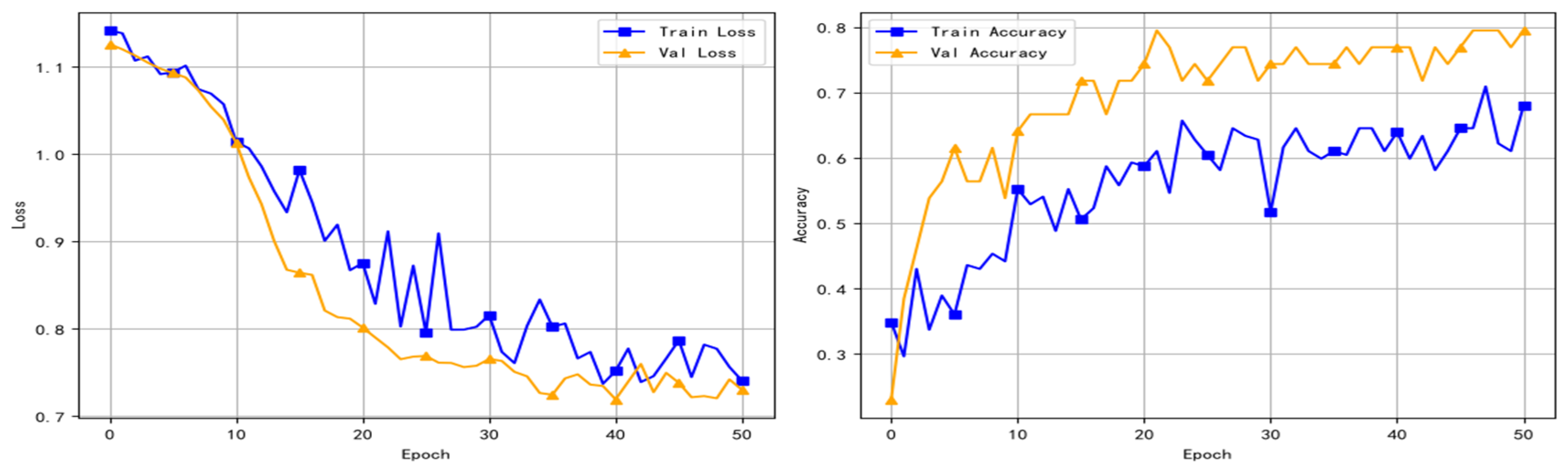
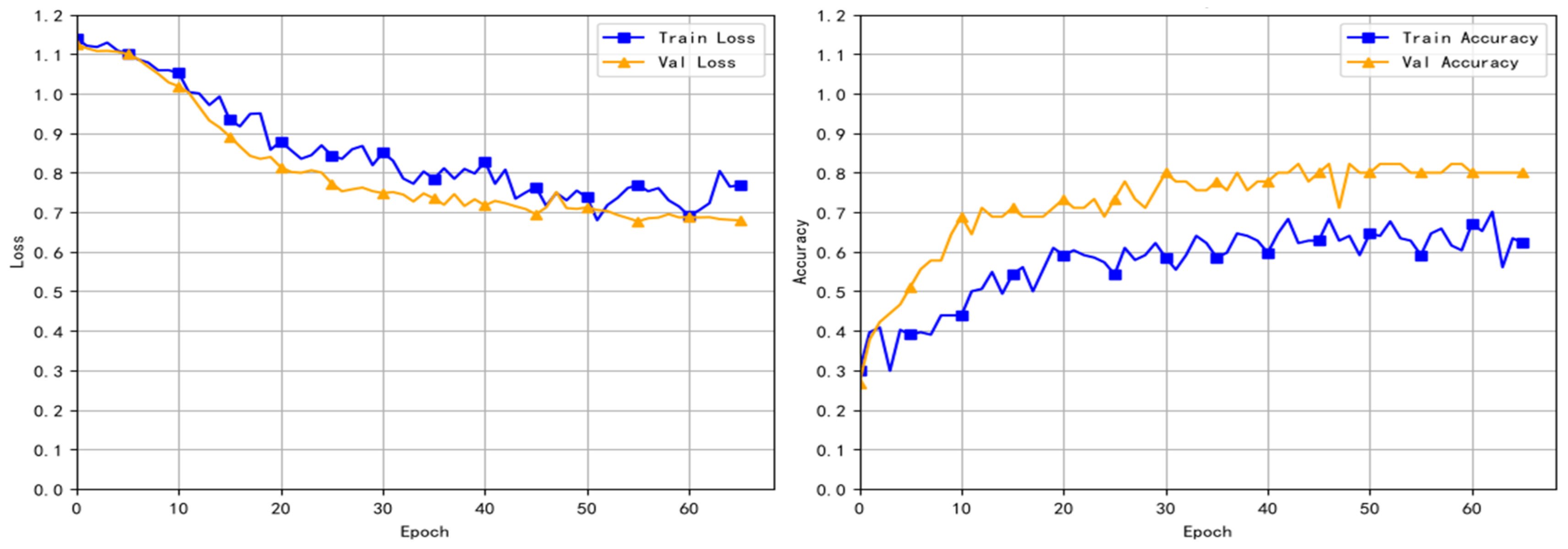
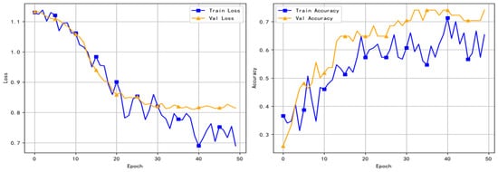
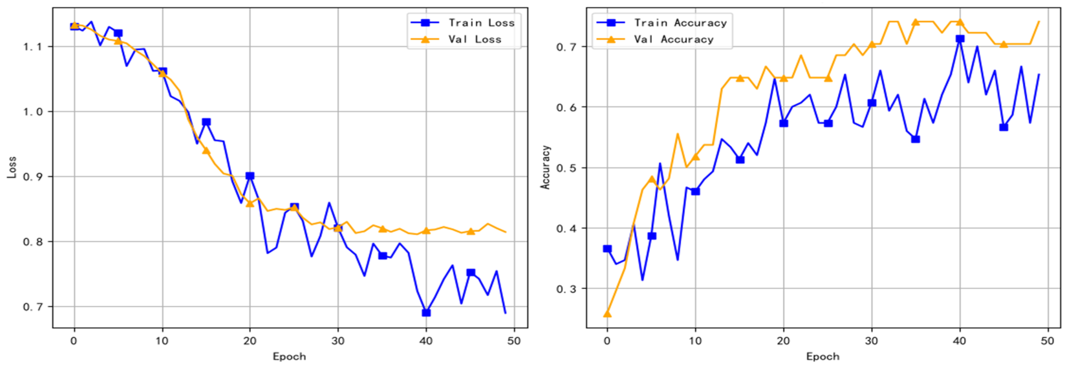
Figure 7, Figure 8 and Figure 9 present the loss curves and accuracy curves when the test set accounts for 25%, 30%, and 35%, respectively. The model trained with a 25% test set split shows insufficient overall classification accuracy and is in a state of mild underfitting. For the model trained with a 35% test set split, the generalization gap between training and validation loss continues to widen after 20 epochs, with obvious overfitting characteristics and poor training robustness. The model trained with a 30% test set split approaches its performance peak at around 40 epochs, and no performance degradation occurs in subsequent iterations. With the early stopping mechanism efficiently locking the optimal weights, it balances convergence adequacy and training efficiency. This further confirms that 30% is the optimal test set split ratio for the CNN-LSTM model. The repeated observation of validation accuracy exceeding training accuracy in Figure 7, Figure 8 and Figure 9 is caused by the high dropout rates (0.6 and 0.5) adopted in the model. During the training phase, dropout layers are activated and randomly deactivate a portion of neurons to suppress overfitting, which lowers the measured training accuracy. When performing validation evaluation, the model switches to inference mode with all dropout layers automatically disabled, and all neurons participate in forward prediction. This leads to slightly higher validation accuracy than training performance. This is a normal occurrence under strong regularization settings, and no data leakage issue exists in our experimental design.
Figure 7.
Loss and accuracy curves with the 75% training set and 25% test set.
Figure 8.
Loss and accuracy curves with the 70% training set and 30% test set.
3.2.2. Robustness Check of the Optimal Training–Test Split
To assess the robustness of the CNN–LSTM model to various time-series partitioning strategies, this study employs two dynamic validation approaches—the Rolling Window and the Expanding Window—for model training. In the Rolling Window setting, a fixed five-year window is designated as the training period, with the subsequent six months utilized as the testing window, ensuring that the termination point of the training set consistently precedes the starting point of the test set. In the Expanding Window approach, the period from February 2012 to December 2020 is designated as the initial training window, followed by a twelve-month testing window. As the validation cycle advances, the training set continuously assimilates newly observed historical data. Both dynamic partitioning schemes not only circumvent the data leakage issues induced by random splitting but also effectively preserve the inherent autocorrelation, seasonality, and lagged economic-cycle effects embedded in the monthly dataset.
Table 4 reports the validation outcomes derived from the Rolling Window and Expanding Window schemes. Although these dynamic strategies are constrained by the fixed window length and sample accumulation, yielding overall macro-averaged F1 scores of 0.6944 and 0.7383, respectively—which are slightly lower than those achieved by the main analysis utilizing the fixed chronological split—they nevertheless confirm the robust early-warning capability of the CNN–LSTM model. Notably, the recall for the High-risk class consistently exceeds 0.92 in both dynamic windows, which is highly consistent with the 1.0 recall observed in the main analysis. This robust consistency underscores that the model maintains reliable performance in capturing high-risk signals, irrespective of the time-series partitioning strategy adopted.
Table 4.
Comparative classification early-warning performance under Rolling and Expanding Window partitioning schemes.
3.2.3. Performance Evaluation Results of the CNN-LSTM Multi-Class Early-Warning Model
Table 5 presents the accuracy, precision, recall, and comprehensive evaluation metric of the CNN-LSTM model in the optimal scenario of a single training run based on the class-wise report with a 30% test set split ratio. To control for the randomness of the CNN-LSTM model and verify its operational robustness, this study runs the model 50 times, with 50 distinct random seeds on the training set and validation set. The summarized results of the performance evaluation metrics, including the mean, standard deviation, and confidence interval, are shown in Table 5 and Table 6 below.
Table 5.
Comparative report on single-run optimal and average early-warning performance.
Table 6.
Class-wise evaluation report on performance stability of the CNN-LSTM model across 50 runs.
Overall, based on the averaged results of the CNN-LSTM model across 50 runs with distinct random seeds, the model achieves a weighted average precision of 0.7843, an overall classification accuracy of 0.7715, and a weighted average F1 score of 0.7536, indicating reliable risk classification capability and stable generalization performance. In particular, the model maintains a recall rate of 0.8933 for the high-risk class: The vast majority of actual high-risk samples in the test set are correctly identified, which effectively guarantees the practical early-warning value of the model for high-risk scenarios. In both the single-run optimal performance report and the average performance report, among the 46 test samples, 23 are consistently classified as low-risk, 11 as medium-risk, and 12 as high-risk. The average results of the CNN-LSTM model across 50 runs exhibit minor discrepancies from the model outputs under the aforementioned optimal scenario. The model produces consistent early-warning judgments on the risk status of the real estate market, which confirms the robustness of the training results. In risk early-warning scenarios, the cost of missing high-risk events is far higher than that of false alarms. The high-recall feature ensures full capture of high-risk events and minimizes potential losses caused by missed warnings. On the core premise of zero missed detection for high-risk events, the model also preserves the discrimination accuracy of low-risk samples. Its performance distribution aligns with the priority setting of risk early-warning tasks, and its overall classification effect meets the application requirements of systemic risk early warning for the “land–real estate–finance” system.
3.2.4. Circular Logic Risk Test Based on the Naive Persistence Benchmark
Given that the low-risk, medium-risk, and high-risk labels are generated from the quantiles of the composite risk index and the predictive input variables for the CNN-LSTM model are fundamentally derived from the same set of underlying market indicators, there is a potential concern that the neural network may merely learn to replicate the deterministic threshold division rules of the index rather than genuinely forecasting independently occurring systemic risk events in reality. To address this issue, this study constructs a Naive Persistence Benchmark for validation. Specifically, this benchmark employs the true risk label at time t as the predicted risk label for time t + 1.
As shown in Table 7, the composite real estate risk index exhibits strong autocorrelation, and the benchmark model also achieves relatively high prediction accuracy under this alternative labeling framework. Nevertheless, the main analytical model still significantly outperforms this benchmark in terms of precision, recall, and F1 score. This finding indicates that the performance of the main analytical model does not stem from learning and reproducing the risk threshold classification rules. Instead, the model extracts information from the underlying fundamental indicators to independently predict the composite risk status of the real estate market.
Table 7.
Performance evaluation report of the Naive Persistence Benchmark.
3.2.5. Robustness Test and Comparative Advantages of the CNN-LSTM Model
To verify the effectiveness of the CNN-LSTM real estate risk early-warning model constructed in this paper, this study selects five mainstream machine learning models, namely CNN, LSTM, random forest, gradient boosting, and PSO-SVM, as benchmarks for comparison. All models are repeatedly run with 50 sets of random seeds under the identical dataset and experimental settings, and their early-warning accuracy and robustness are comprehensively evaluated based on average performance metrics and standard deviations. The results are shown in Table 8.
Table 8.
Performance comparison between CNN-LSTM and other machine learning models.
PSO-SVM automatically optimizes SVM hyperparameters through the particle swarm optimization algorithm, which avoids the subjectivity of manual parameter tuning. However, the empirical results show that all its performance metrics rank the lowest, with standard deviations significantly higher than those of other models. This indicates that the model is sensitive to fluctuations in sample data distribution and suffers from insufficient generalization stability. The random forest model constructs a parallel ensemble of multiple decision trees under the Bagging framework, which inherently possesses anti-overfitting properties. Its standard deviations remain at a low level, reflecting sound parameter robustness. Nevertheless, the tree-based structure struggles to capture the temporal dependency of risks and cannot fully explore the dynamic evolution law of risk transmission, resulting in a moderate overall early-warning performance. The single CNN model extracts local correlation patterns among features via one-dimensional convolution kernels, and performs well in identifying contemporaneous multi-dimensional risk coupling features, with slightly better performance than the random forest. However, the convolution structure lacks long-sequence memory capability, making it difficult to capture the transmission trend of risks in the temporal dimension and entailing inherent modeling limitations. The single LSTM model realizes long-term memory of temporal information through its gating mechanism, which fits the modeling characteristics of sequential data. Its F1 score reaches 0.701, outperforming the single CNN model, which corroborates the core value of temporal dependency features in real estate risk early warning. Nonetheless, LSTM has weak capability in extracting local fine-grained features and cannot deeply explore the nonlinear correlations among contemporaneous indicators. The gradient boosting model continuously improves classification performance by serially fitting residuals, with strong fitting capacity and early-warning accuracy close to that of the single LSTM. However, its serial training mechanism is susceptible to random fluctuations, leading to relatively higher standard deviations.
The hybrid CNN-LSTM model proposed in this paper integrates the structural advantages of the two deep learning architectures. Its overall performance metrics outperform all comparative models, while the standard deviations of all indicators remain around 0.05, maintaining robust early-warning performance. The model can not only accurately identify high-risk samples but also maintain stable performance under different random conditions. It effectively adapts to the complex features of multi-dimensional coupling in the real estate market risk system and holds practical application value.
3.2.6. Risk Early-Warning Results of the CNN-LSTM Model
Within the CNN-LSTM framework, the CNN module excels at capturing short-term fluctuations in time series through convolution operations, while the LSTM module is designed to identify long-term trends. The convolution kernel in the CNN module (kernel_size = 3) slides strictly along the feature sequence direction, covering three adjacent feature positions at each step to learn short-term correlation patterns between locally adjacent features within a single-month sequence. The MaxPooling1D layer (pool_size = 2) further downsamples the local features, enhancing the capture of local fluctuation patterns. Subsequently, the LSTM module receives the local feature sequence extracted by the CNN module and performs recursive operations along the sequence dimension through its gated recurrent units (input gate, forget gate, and output gate), modeling global dependencies from the beginning to the end of the sequence and thereby identifying long-term structural patterns that span the entire feature sequence. Together, the two modules form a hierarchical structure of “local feature extraction–global temporal modeling. Trained on historical data, the CNN-LSTM model can generate monthly forecasts of real estate risk status changes. When the feature data for February, March, and April 2026 are fed into the model, the corresponding early-warning results for March, April, and May 2026 are output, all indicating a medium risk level. According to data from the National Bureau of Statistics of China, China’s real estate market exhibited marked regional disparities in early 2026. Some first-tier cities showed strong resilience: Transaction volume rebounded in core areas, the number of listed second-hand homes fell notably, and month-on-month prices stopped declining and registered a slight increase. In contrast, third- and fourth-tier cities still faced substantial destocking pressure, with prolonged inventory digestion cycles in some cities and a “price-for-volume” pattern in second-hand housing transactions. Many local authorities have introduced measures, including preferential housing mortgage policies, housing “trade-in” programs, and state-owned enterprise purchases of existing housing stock for affordable housing, in an effort to unblock the housing replacement chain and reduce inventory. The overall performance of the national real estate market is broadly consistent with the predicted risk status.
To further verify the credibility of the early-warning results, the sample’s end date is extended from December 2025 (adopted in the preceding analysis) to May 2026, and a new composite sample index is constructed. As shown in Table 9, the risk status labeled by the new composite index synthesized from actual data is consistent with the risk status predicted by the trained CNN-LSTM model in this study, which further validates the robustness and generalization capability of the early-warning model. This 3-month out-of-sample data validation serves only as supplementary reference for the model’s generalization performance, rather than being a core component of performance evaluation. The core conclusions of this paper remain strictly based on the averaged test-set results across multiple random seeds.
Table 9.
Comparison between risk status labeled by composite index and output results of the CNN-LSTM early-warning model.
4. Conclusions
From the perspective of risk linkage and transmission across the “land–real estate–finance” system, this paper constructs a two-tier framework of a coupled risk monitoring indicator system for the real estate market, introduces the BEKK-GARCH time-varying coefficient matrix to synthesize a comprehensive real estate risk index, and realizes the multi-class early warning of systemic risk in the real estate market based on the CNN-LSTM model. The design of the indicator system and the specification of the adaptive machine learning model in this study are primarily developed based on samples from China’s real estate market. The external generalizability of the model’s risk early-warning capability remains to be validated with samples from more countries and regions.
From the perspective of cross-market risk contagion and comprehensive prevention and governance of the “land–real estate–finance” system, this paper puts forward the following suggestions:
- For risk prevention in the land market, it is necessary to build a flexible and adaptive land supply mechanism to curb price fluctuations caused by supply–demand mismatch. Core indicators such as land transaction prices, premium rates, unsold auction rates, and land supply pace should be incorporated into regular monitoring. Standardize land mortgage financing operations, strictly prohibit illegal amplification of land financing leverage through urban investment platforms, and prevent the risk of collateral depreciation caused by falling land values from transmitting to local government debt and the banking system.
- For risk prevention in the real estate market, authorities should promptly address public concerns in response to market risk events and precisely resolve debt risks of key real estate enterprises through market-oriented approaches to prevent individual risks from spreading to the entire industry and stabilize expectations of market entities and homebuyers. In the era of stock housing, real estate enterprises should be guided to explore the transformation to asset-light operation models and encouraged to extend value-added service chains such as housing services, urban operation, and asset management so as to broaden funding sources and foster sustainable profit models.
- For risk prevention in the housing-related financial market, bottlenecks and blockages restricting the entry of medium- and long-term capital into the market should be removed, and enterprises should be supported to expand financing channels and improve efficiency through bonds, equities, REITs and other instruments. Improve the macro-prudential management system for real estate finance, dynamically adjust credit policies and financing thresholds in line with market cycles, and mitigate the amplification effect of financial market shocks on real estate risks through counter-cyclical adjustment.
- To prevent cross-market risk spillovers across the “land–real estate–finance” system, it is recommended to reduce local governments’ dependence on land finance, curb irrational land acquisition by developers and land price bubbles, and weaken the transmission impact of land price fluctuations on real estate and financial markets.
- Based on the three-tier risk early-warning system for the real estate market, a gradient regulation framework should be established to achieve precise matching between risk levels and regulation intensity: (1) Under the low-risk state, the core focus lies in regularized supervision and long-term mechanism development. On the policy front, it is necessary to strengthen cross-departmental market monitoring and expectation guidance, maintain a balanced pace of land supply, and enforce routine compliance supervision over the market. On the financial front, priority should be given to supporting rigid and improvement housing demand, and quarterly real estate credit stress tests should be conducted to identify potential risks in advance. (2) Under the medium-risk state, the target is to contain risk diffusion in a targeted manner. On the policy front, city-specific regulatory policies should be implemented, with targeted adjustments to land supply in regions with rising risks. On the financial front, differentiated housing credit policies should be adopted, window guidance on financing should be imposed on highly leveraged real estate enterprises, a financing whitelist for guaranteed housing delivery should be established, and stock risks should be resolved through market-oriented approaches such as asset securitization. (3) Under the high-risk state, the bottom line of preventing systemic risks must be firmly upheld. Multi-departmental coordination is required to build an emergency response mechanism for the coupled risks across the land, real estate, and financial sectors. On the supply side, state-owned enterprises should act as market backstops to stabilize the land market, and enterprise-specific solutions should be formulated for distressed leading real estate enterprises. On the financial front, special re-lending facilities and bailout funds should be set up, asset management companies should be introduced for the batch disposal of non-performing assets, and risk mitigation tools should be deployed to block cross-market risk transmission channels and prevent risk spillover from individual markets.
Constrained by data statistical frequency and sample availability, this study still has several limitations. First, subject to the statistical rules of national macro-real estate indicators, the empirical samples in this paper adopt monthly data, making it difficult to capture the intra-month evolution characteristics of risks in real time. In addition, the limited sample size restricts the potential of the CNN-LSTM model in mining complex nonlinear patterns to a certain extent. With the improvement of the digital governance system and the advancement of big data technology, access to higher-frequency daily data in future research will further improve the prediction accuracy of the CNN-LSTM model. Second, considering that China’s real estate market has not been hit by extreme risk events throughout the sample period, Extreme Value Theory (EVT) is not introduced into the deep learning model due to the lack of training samples. The existing model can only identify tail extreme risk events as high-risk zones and has not yet achieved separate delineation of higher-level early-warning regimes.
Author Contributions
Conceptualization, W.W. and G.C.; methodology, W.W. and G.C.; software, W.W.; validation, G.C.; formal analysis, W.W.; data curation, W.W.; writing—original draft preparation, W.W. and G.C.; writing—review and editing, W.W. and G.C.; visualization, W.W.; funding acquisition, W.W. All authors have read and agreed to the published version of the manuscript.
Funding
This research was funded by the Ministry of Education of China Humanities and Social Sciences Project (No. 21YJC790124) and the National Social Science Fund of China (No. 22BJY233).
Data Availability Statement
The raw data supporting the conclusions of this article will be made available by the authors upon request.
Conflicts of Interest
The authors declare no conflicts of interest.
Notes
| 1 | The land premium rate measures the relative extent to which the final transaction price of a land parcel surpasses its initial price. It serves as a key leading indicator for evaluating the prosperity of the real estate market. A higher premium rate reflects more intense competition among developers in land acquisition and more optimistic expectations for the subsequent real estate market. The formula is as follows:
|
| 2 | January data are missing for each year of the sample period, as the National Bureau of Statistics suspends data release in January to account for the Spring Festival effect. |
| 3 | The combined weighting coefficient β = 0.5 is designed to give balanced consideration to the weighting logics of the CRITIC method and the entropy weight method, and the results of risk status identification are not highly sensitive to minor variations in the value of β. |
| 4 | Since official GDP data in China are published only on a quarterly basis and industrial operation constitutes a core component of China’s macroeconomic fluctuations, the industrial value-added indicator is a commonly used proxy for monthly macroeconomic fundamentals. |
| 5 | Detailed comparisons are not elaborated herein due to space limitations and are available upon request. |
References
- Adrian, T.; Brunnermeier, M.K. CoVaR. Am. Econ. Rev. 2016, 106, 1705–1741. [Google Scholar] [CrossRef] [Scilit]
- Bernanke, B.; Gertler, M.; Gilchrist, S. The financial accelerator in a quantitative business cycle framework. Handb. Macroecon. 1999, 15, 1341–1393. [Google Scholar] [CrossRef] [Scilit]
- Davis, M.A.; Larson, W.D.; Oliner, S.D.; Smith, B.R. A Quarter Century of Mortgage Risk. Rev. Financ. 2023, 27, 581–618. [Google Scholar] [CrossRef] [Scilit]
- Bckman, C.; Lutz, C. Mortgage innovation and house price booms. J. Urban Econ. 2025, 145, 103725. [Google Scholar] [CrossRef] [Scilit]
- Greenwald, D.L.; Guren, A. Do Credit Conditions Move House Prices? Am. Econ. Rev. 2025, 115, 3559–3596. [Google Scholar] [CrossRef] [Scilit]
- Smith, C.L.B. “Public Land Banking and the Price of Land”: Reply. Land Econ. 1976, 52, 565–566. [Google Scholar] [CrossRef] [Scilit]
- Lee, S.Y. Monetary policy transmission over house price cycles. Empir. Econ. 2025, 69, 3183–3204. [Google Scholar] [CrossRef] [Scilit]
- Grimes, A.; Aitken, A. Housing Supply, Land Costs and Price Adjustment. Real Estate Econ. 2010, 38, 325–353. [Google Scholar] [CrossRef] [Scilit]
- Crossley, T.F.; Levell, P.; Low, H. House price rises and borrowing to invest. J. Econ. Behav. Organ. 2024, 223, 86–105. [Google Scholar] [CrossRef] [Scilit]
- Ahmed, I.; Socci, C.; Medabesh, A.; Severini, F.; Zotti, J. Economic impact of monetary policy: Focus on real estate sector in Italy. Int. J. Financ. Econ. 2021, 26, 1256–1269. [Google Scholar] [CrossRef] [Scilit]
- Chen, J.; Wu, F. Housing and land financialization under the state ownership of land in China. Land Use Policy 2022, 112, 104844. [Google Scholar] [CrossRef] [Scilit]
- Li, S.; Pan, H.; Chen, J. Pathways out of land financialization: Understanding transformation strategies of urban investment insolvency and crisis. Urban Stud. 2026, 63, 700–719. [Google Scholar] [CrossRef] [Scilit]
- Xiao, Z.; Zhang, H. Real estate market regulation and local government debt risk. Financ. Res. Lett. 2025, 80, 107362. [Google Scholar] [CrossRef] [Scilit]
- Su, Y.X.; Shi, S.; Hu, M.Z.; Wu, Y.Z. Land financialization and gentrification: Evidence from China. Cities 2024, 154, 105330. [Google Scholar] [CrossRef] [Scilit]
- Wang, J.H. Sustainable Land-Use Policy: Land Price Circuit Breaker. Sustainability 2025, 17, 11232. [Google Scholar] [CrossRef] [Scilit]
- Lewis, D.; Springer, T.M.; Anderson, R.I. The Cost Efficiency of Real Estate Investment Trusts: An Analysis with a Bayesian Stochastic Frontier Model. J. Real Estate Financ. Econ. 2003, 26, 65–80. [Google Scholar] [CrossRef] [Scilit]
- Guo, F.; Chen, C.R.; Huang, Y.S. Markets contagion during financial crisis: A regime-switching approach. Int. Rev. Econ. Financ. 2011, 20, 95–109. [Google Scholar] [CrossRef] [Scilit]
- Ma, Y.; Liu, C. Real Estate Market Price Fluctuation and Instrument Rules Choice of China’s Monetary Policy——Analysis Based on the DSGE Model. Stud. Int. Financ. 2014, 8, 24–34. [Google Scholar]
- Wei, W.; Chen, J. The Impact of Agricultural Hukou on Migrants’ Home Purchasing in Destination Cities of China. Sustainability 2025, 17, 11072. [Google Scholar] [CrossRef] [Scilit]
- Anundsen, A.K.; Gerdrup, K.; Hansen, F.; Kragh-Sorensen, K. Bubbles and Crises: The Role of House Prices and Credit. J. Appl. Econom. 2016, 31, 1291–1311. [Google Scholar] [CrossRef] [Scilit]
- Levantesi, S.; Piscopo, G. The Importance of Economic Variables on London Real Estate Market: A Random Forest Approach. Risks 2020, 8, 112. [Google Scholar] [CrossRef] [Scilit]
- Wang, X.J.; Zeng, G.T.; Zhang, K.X.; Chu, H.B.; Chen, Z.S. Urban Real Estate Market Early Warning Based on Support Vector Machine: A Case Study of Beijing. Int. J. Comput. Intell. Syst. 2020, 13, 153–166. [Google Scholar] [CrossRef] [Scilit]
- Zhou, W.W.; Chen, M.Y.; Yang, Z.L.; Song, X.B. Real estate risk measurement and early warning based on PSO-SVM. Socio-Econ. Plan. Sci. 2021, 77, 101001. [Google Scholar] [CrossRef] [Scilit]
- Jozko, M.; Vergos, K. Comparing Var and Artificial Neural Network Model in Forecasting Real Estate Prices during Good and Bad Times. Preprints 2024. [Google Scholar] [CrossRef] [Scilit]
- Davis, J.; Devos, L.; Reyners, S.; Schoutens, W. Gradient boosting for quantitative finance. J. Comput. Financ. 2021, 24, 24. [Google Scholar] [CrossRef] [Scilit]
- Giantsidi, S.; Tarantola, C. Deep learning for financial forecasting: A review of recent trends. Int. Rev. Econ. Financ. 2025, 104, 104719. [Google Scholar] [CrossRef] [Scilit]
- Cao, G.X.; Ling, M.J.; Wei, J.W.; Chen, C. Dynamic market behavior and price prediction in cryptocurrency: An analysis based on asymmetric herding effects and LSTM. Comput. Econ. 2025, 65, 3325–3360. [Google Scholar] [CrossRef] [Scilit]
- Borovkova, S.; Tsiamas, I. An ensemble of LSTM neural networks for high-frequency stock market classification. J. Forecast. 2019, 38, 600–619. [Google Scholar] [CrossRef] [Scilit]
- Chen, T.; Kung, K.S. Busting the ‘Princelings’: The Campaign Against Corruption in China’s Primary Land Market. Q. J. Econ. 2019, 134, 185–226. [Google Scholar] [CrossRef] [Scilit]
- Cho, S.; Jung, J. Behavioral Finance Insights into Land Management: Decision Aggregation and Real Estate Market Dynamics in China. Land 2024, 13, 1478. [Google Scholar] [CrossRef] [Scilit]
- Ngai, L.R.; Sheedy, K.D. The Ins and Outs of Selling Houses: Understanding Housing-Market Volatility. Int. Econ. Rev. 2024, 65, 1415–1440. [Google Scholar] [CrossRef] [Scilit]
- Bourassa, S.C.; Haurin, D.R.; Haurin, J.L.; Hoesli, M.; Sun, J. House Price Changes and Idiosyncratic Risk: The Impact of Property Characteristics. Real Estate Econ. 2009, 37, 259–278. [Google Scholar] [CrossRef] [Scilit]
- Margulis, H.L. Suburban Housing Resale Prices and Housing Market Restructuring. J. Urban Aff. 2010, 24, 461–477. [Google Scholar] [CrossRef] [Scilit]
- Hosios, A.J.; Pesando, J.E. Measuring prices in resale housing markets in Canada: Evidence and implications. J. Hous. Econ. 1991, 1, 303–317. [Google Scholar] [CrossRef] [Scilit]
- Bourassa, S.C.; Hoesli, M.; Oikarinen, E. Measuring House Price Bubbles. Real Estate Econ. 2016, 47, 534–563. [Google Scholar] [CrossRef] [Scilit]
- Ke, S.; Lu, X. Real Estate Investment, Loan Preference, and National Happiness: Evidence from China. Land 2021, 10, 428. [Google Scholar] [CrossRef] [Scilit]
- Mian, A.R.; Sufi, A. The Consequences of Mortgage Credit Expansion: Evidence from the U.S. Mortgage Default Crisis. Q. J. Econ. 2009, 124, 1449–1496. [Google Scholar] [CrossRef] [Scilit]
- Kremer, M.; Duca, M.L.; Holló, D. CISS—A Composite Indicator of Systemic Stress in the Financial System. SSRN Electron. J. 2012, 1, 347–351. [Google Scholar] [CrossRef] [Scilit]
- Louzis, D.P.; Vouldis, A.T. A methodology for constructing a financial systemic stress index: An application to Greece. Econ. Model. 2012, 29, 1228–1241. [Google Scholar] [CrossRef] [Scilit]
- Wei, W.; Wu, F. Research on Four-Dimensional Monitoring and Early Warning of Real Estate Market Risks. Financ. Regul. Res. 2025, 12, 47–61. [Google Scholar] [CrossRef]
- Yang, G.Y.; Wang, Z. Measurement of Systemic Financial Risk Based on Quantile Factor Analysis. Wuhan Financ. 2023, 8, 33–40. [Google Scholar]
- Zeng, Z.F.; You, Y. Financial Risk Early Warning Based on Neural Network Quantile Regression. Stat. Decis. 2020, 36, 137–140. [Google Scholar] [CrossRef]
- Li, M. Construction of Systemic Financial Stress Index Based on Three-Step Regression Filtering Model. Stat. Decis. 2022, 38, 131–135. [Google Scholar] [CrossRef]

Disclaimer/Publisher’s Note: The statements, opinions and data contained in all publications are solely those of the individual author(s) and contributor(s) and not of MDPI and/or the editor(s). MDPI and/or the editor(s) disclaim responsibility for any injury to people or property resulting from any ideas, methods, instructions or products referred to in the content. |
© 2026 by the authors. Licensee MDPI, Basel, Switzerland. This article is an open access article distributed under the terms and conditions of the Creative Commons Attribution (CC BY) license.