


Abstract
Weekday commuting and weekend recreation are two mobility domains through which urban spatial structure affects residents’ daily experience and urban functioning. Although commuting and recreational mobility are theoretically related, whether their spatial relationship creates scope for coordinated improvement in both domains remains insufficiently understood. A preceding study in Chongqing identified a U-shaped relationship between weekday commuting costs and weekend recreational mobility costs at the individual level, but its proposed spatial-structural interpretation remained untested. This study examines whether the same relationship emerges across residential locations and whether the resulting mobility-cost structure corresponds to the spatial configuration of employment and recreational opportunities. Using location-based services data from the central urban area of Chongqing, individual mobility records were aggregated to residential grids and analysed through a three-stage framework examining the grid-level U-shaped relationship, multivariate dependence between the opportunity and cost structures, and their curve-based correspondence. The U-shaped relationship was reproduced at the grid level. The opportunity and cost structures exhibited multivariate dependence, and the curve-based analysis showed a positive correspondence between residential grids’ positions relative to the fitted opportunity and cost reference points. These findings support the interpretation that the U-shaped relationship partly reflects how residential locations are positioned relative to multiple employment centres and spatially distributed recreational destinations. The findings indicate that commuting and recreational mobility should be considered jointly in jobs–housing–recreation planning and suggest potential scope for coordinated improvement across both domains.
1. Introduction
Weekday commuting and weekend recreation are two major domains of intra-urban mobility through which urban spatial structure affects residents’ daily experience and the functioning of cities. Commuting represents the most regular and largely unavoidable form of work-related travel, whereas recreational mobility reflects access to leisure, recovery, social interaction, and other non-work activities. Both are anchored in residential location and shaped by the spatial distribution of employment, housing, and recreational resources. They should therefore be considered jointly when examining how urban spatial structure shapes residents’ combined work-related and non-work mobility conditions.
The value of a joint commuting–recreation perspective lies in addressing both an imbalance in existing research and the practical interdependence of the two mobility domains. Commuting has long been central to research on jobs–housing balance, spatial mismatch, excess commuting, and urban accessibility [1,2,3,4,5,6,7,8]. Recreational mobility has received comparatively less attention, despite its importance for quality of life, leisure participation, social interaction, and the attractiveness of large cities [9,10,11]. This imbalance is increasingly difficult to justify in large Chinese cities, where congestion extends beyond weekday commuting peaks into weekend leisure periods and recreational travel has become an important component of urban mobility. Moreover, commuting and recreation are interrelated rather than independent. Households may value open spaces, leisure facilities, environmental quality, social contacts, and other non-work amenities when choosing where to live, and these preferences may affect the commuting costs they subsequently bear [12,13]. The relevant planning question is therefore not only whether jobs and housing are balanced, but how jobs, housing, and recreation are jointly configured to shape combinations of work-related and non-work mobility conditions.
Existing research provides important foundations for a joint commuting–recreation perspective, but it generally remains organised around separate opportunity–outcome relationships. Commuting-centred studies examine how employment accessibility and urban spatial structure influence commuting time, distance, and excess commuting [1,2,3,4,5,6,8]. Such studies rarely consider realised non-work travel; when recreational amenities are included, they are usually treated as attributes of residential location rather than as mobility outcomes. Recreation-related research focuses on the accessibility, equity, quality, and use of parks, greenspaces, and other leisure resources, increasingly using human-mobility data to evaluate actual visitation [14,15,16,17,18,19,20]. Studies of non-work travel further examine activity types and nonlinear built-environment associations [21]. Residential-location research considers trade-offs among a broad range of residential amenities and locational attributes, including housing characteristics, commuting burdens, neighbourhood conditions, employment accessibility, open-space access, leisure facilities, and social contacts [12,13,22,23,24,25]. Built-environment and mixed-use studies likewise assess how density, diversity, design, destination accessibility, and transit access shape travel behaviour, often treating lower commuting burdens and improved access to non-work opportunities as parallel benefits of integrated land-use arrangements [26,27,28].
Taken together, these four strands indicate that commuting performance, recreational access and use, residential-location trade-offs, and built-environment effects on travel are conceptually connected. Yet research within these strands remains organised around distinct analytical foci and generally studies commuting and recreational mobility in separate analytical frames rather than examining their relationship directly. Consequently, these strands do not establish whether weekday commuting costs and weekend recreational mobility conditions are related, what form any such relationship takes, or how it may be grounded in the underlying jobs–housing–recreation spatial structure. Resolving these questions is fundamental to evaluating the joint mobility performance of jobs–housing–recreation spatial structure and providing an empirical basis for coordinated improvements in commuting and recreational mobility conditions.
Our previous individual-level study identified a U-shaped relationship between weekday commuting costs and weekend recreational mobility conditions [29]. Individuals with moderate commuting costs tended to travel shorter distances or times for weekend recreation, whereas those with shorter or longer commutes tended to travel farther or longer. The study interpreted this relationship within a jobs–housing–recreation spatial framework, but that interpretation was not tested using spatial evidence.
The proposed interpretation has two testable spatial implications. First, the U-shaped relationship identified among individuals should also be observable across residential locations. Second, the resulting grid-level relationship should correspond to how residential locations are positioned relative to employment centres and recreational destinations. Together, these implications provide a spatial test of whether the observed commuting–recreation relationship is consistent with the broader organisation of jobs, housing, and recreation.
Accordingly, this study addresses two research questions:
- Does the individual-level U-shaped relationship between commuting and recreational mobility costs also emerge at the residential-grid level (RQ1)?
- Does the grid-level commuting–recreation relationship correspond to the spatial relationship between employment-centre proximity and recreational opportunity (RQ2)?
To answer these questions, the study uses 1 km residential grids in the central urban area of Chongqing, China. It first examines whether the U-shaped relationship is reproduced across residential grids, then assesses multivariate dependence between the employment–recreation opportunity structure and the commuting–recreation cost structure, and finally evaluates whether the specific form of their correspondence is consistent with the proposed spatial hypothesis.
This study extends the preceding individual-level analysis by shifting the focus from the observed individual mobility association to its residential-grid manifestation and spatial-structural correspondence. It first establishes whether the U-shaped relationship has a residential-grid counterpart and then tests whether that spatial pattern corresponds to the jobs–housing–recreation spatial structure. By assessing whether the observed mobility relationship has a spatial-structural basis, the study provides new spatial evidence on the relationship between commuting and recreational mobility, thereby clarifying why both domains should be considered jointly in jobs–housing–recreation planning and where coordinated improvement may be possible.
2. Materials and Methods
2.1. Conceptual Definitions and Analytical Unit
Three concepts are central to the analysis: weekday commuting costs, weekend recreational activities, and weekend recreational mobility conditions. In the subsequent analysis, the distance- and time-based indicators used to represent recreational mobility conditions are referred to as recreational mobility costs.
First, weekday commuting costs refer to the time- and distance-based burdens of regular home–work travel on weekdays. In this study, commuting is treated as a recurrent and relatively fixed domain of daily mobility, structured by the spatial relationship between residence and workplace. As a necessary activity, its cost reflects the routine travel burden imposed by the existing jobs–housing arrangement.
Second, weekend recreational activities refer to non-work, discretionary activities undertaken during weekends for leisure, relaxation, entertainment, or social participation. This definition excludes work-related trips, weekday after-work activities, and non-work stops embedded in commuting chains. The focus is therefore on recreational behaviour as an independent activity domain rather than an extension of weekday work routines.
Third, weekend recreational mobility conditions refer to the realised travel conditions associated with weekend recreational trips. In this study, they are represented by travel distance and travel time between the individual’s residence and identified recreational destinations for home-based weekend recreational trips, rather than by subjective evaluation or potential accessibility alone.
Although commuting and recreational mobility are first measured at the individual level, the analytical unit of the present study is the residence-based spatial grid. Individual mobility records are aggregated according to residence location, so that each grid is characterised by its employment and recreational-opportunity conditions and the associated commuting and recreational mobility costs. The opportunity conditions refer broadly to the employment and recreational resources available from each residential location; their analytical representation and measurement are specified in Section 2.3 and Section 2.4.3. The construction and aggregation of the residential grids are described in Section 2.4.
2.2. Study Area, Data, and Individual-Level Mobility Measures
2.2.1. Study Area
Consistent with the preceding individual-level study [29], the central urban area of Chongqing (Figure 1) was selected as the study area. It contains a large population, intensive weekday and weekend travel demand, and a complex spatial arrangement of residential neighbourhoods, employment centres, commercial facilities, parks, cultural venues, and other recreational destinations. These characteristics generate substantial spatial variation in both home–work commuting conditions and weekend recreational mobility. The case is also relevant to the broader planning problem addressed in this study: as in many large Chinese metropolitan areas, mobility pressures in Chongqing are no longer confined to weekday commuting peaks, with congestion increasingly extending into weekends.
Figure 1.
Study area and spatial context of the Chongqing central urban area. Red and blue lines in panel (c) indicate national and maritime boundary lines, respectively. Reproduced from the preceding individual-level study [29].
Using the same urban context allows the present analysis to extend the preceding evidence from individuals to residential locations while holding the broader metropolitan setting constant. This continuity makes it possible to assess whether the previously identified U-shaped relationship has a residential-grid manifestation and whether that manifestation is consistent with its proposed spatial-structural interpretation.
2.2.2. Data Source and Observation Period
Location-based services (LBS) data were used to capture individual-level commuting and recreational mobility. The dataset consisted of anonymised and de-identified location records derived from GPS- and Wi-Fi-based positioning, and no direct personal identifiers were available to the authors. Stable residence and workplace locations were provided by the data vendor as pre-identified attributes inferred from a three-month observation window; the identification rules are described in Section 2.2.3. The distributions of residents and workers represented in the dataset were highly consistent with official population and economic census distributions at the sub-district level in Chongqing, supporting their use for constructing spatially aggregated mobility indicators.
The records used to construct the commuting and recreational indicators covered the period from 30 October 2023 to 3 December 2023. This period fell mainly in November, when recreational activity in Chongqing was less likely to be strongly constrained by extreme heat or cold. Nevertheless, a single observation period cannot fully capture seasonal variation; this limitation is discussed further in Section 4.
The subsequent data-processing procedure comprised the identification of weekend recreational visits, construction and screening of individual-level mobility measures, aggregation to residence-based grid cells, and formation of the stage-specific analytical samples. Figure 2 provides an overview of this workflow; the individual-level procedures are detailed in Section 2.2.3 and Section 2.2.4, and the grid-level aggregation and variable construction are described in Section 2.4.
Figure 2.
Workflow for constructing and screening the stage-specific residential-grid analytical samples from anonymised location-based services records.
2.2.3. Identification of Residence, Workplace, and Weekend Recreational Visits
According to the data vendor’s processing rules, residence refers to the dominant nighttime location during 22:00–07:00, while workplace refers to the dominant weekday daytime location during 10:00–17:00. These vendor-derived locations were used directly rather than re-identified by the authors.
Weekend recreational visits were identified using an area-of-interest (AOI)-based approach. The selected AOI categories served as observable proxies for the recreational activities defined in Section 2.1 and included shopping, tourist attractions, leisure and entertainment, and cultural services, as detailed in Appendix A, Table A1. A weekend visit was recorded when an individual’s location points fell within one of these AOIs during the observation window. To reduce misclassification, visits to AOIs located within 500 m of the individual’s workplace were excluded. This exclusion reduced the inclusion of work-related presence, routine stops, and incidental activities. In the subsequent construction of mobility measures, the remaining AOIs were treated as destinations of home-based weekend recreational trips originating from the individual’s residence. The distribution of the number of distinct recreational AOIs identified per person-day is reported in Appendix A, Table A2.
2.2.4. Route-Based Mobility Measures and Analytical Sample Construction
Route-based measures were constructed for the identified commuting OD pairs and recreational-visit OD pairs. The LBS data allow the identification of activity locations and origin–destination relationships, but do not directly observe realised travel routes, travel time, or travel mode. Route distance and mode-specific travel times were therefore estimated using the Baidu Maps Web Service APIs. Specifically, DirectionLite v1 was used to obtain driving-route distances and driving times, whereas Direction v2 was used to obtain transit times. The APIs were queried under the temporal settings specified below.
For commuting, route distance and driving and transit times were retrieved for each individual’s stable residence–workplace OD pair during weekday peak periods (07:30–09:30 and 17:30–19:30) to represent typical commuting conditions. For recreation, route distance and driving and transit times were retrieved for each OD pair between the residence and an identified recreational destination during weekend daytime periods (10:30–19:00), corresponding to the main temporal window of recreational activity. Because the actual travel mode of each observed visit cannot be reliably identified from the LBS data, the mode-specific travel times are treated as alternative route-based measures of mobility conditions rather than direct observations of realised mode choice.
Accordingly, commuting and recreational mobility denote the activity domains under study rather than observed travel modes. In the analytical variables, driving refers specifically to API-derived driving-time measures. Route distance was obtained using the same driving-routing option to provide a consistent road-network measure of origin–destination separation; this does not imply that the observed trip was made by car. Public-transport travel time was not used to construct any of the four core variables in the main spatial analyses.
Commuting measures were constructed from each individual’s stable residence–workplace OD pair, whereas recreational measures were constructed from residence–destination pairs associated with identified weekend recreational visits. When multiple weekend recreational visits were observed for the same individual, visit-level recreational measures were aggregated to the individual level using mean values.
To maintain comparability with the preceding individual-level study [29], the same sample-screening rules were retained. Several filtering criteria were applied to ensure that weekday commuting patterns and weekend recreational mobility could be consistently identified. Individuals without regular commuting were excluded, including those without a stable workplace and those whose residence and dominant daytime activity locations coincided within campus-type areas. Such cases do not provide a reliable basis for identifying conventional weekday home–work commuting. Individuals flagged by the data vendor as scenic-area staff were also excluded because their presence at recreational destinations could not be reliably distinguished from work-related activity. This occupational flag was used solely for sample screening and was not included in the subsequent analysis.
The analysis was subsequently restricted to complete cases with all measures required for the spatial analysis. To keep the analysis within the principal empirical range of ordinary intra-urban mobility conditions, observations involving driving-time or transit-time measures greater than 90 min were excluded. Observations with commuting or recreational distance greater than 30 km were also excluded. The 30 km threshold corresponded approximately to the 99th percentile of the sample distribution and excluded a small number of exceptionally long trips while preserving the principal empirical range of intra-urban mobility. Together, these steps defined a sample consistent with that used in the preceding individual-level study [29], which was subsequently aggregated to residential grids.
2.2.5. Comparability with and Distinction from the Preceding Individual-Level Sample
This individual-level screening procedure was intentionally kept consistent with the preceding individual-level study [29] to ensure comparability between the individual-level findings and the present spatial test. The two studies therefore share the same underlying individual mobility sample and the same individual-level exclusion rules. However, the analytical sample used in the present study is not the individual sample itself. The screened individual records were aggregated to residence-based 1 km grids, and the subsequent analysis was conducted on the resulting residential-grid sample. From this point onward, the present study differs from the preceding individual-level study [29] in its analytical unit, spatial variables, and empirical design: it constructs grid-level commuting and recreational mobility costs, employment-centre proximity, and recreational opportunity, and then evaluates their multivariate and curve-based correspondence.
2.3. Analytical Framework and Inferential Scope
Figure 3 formalises the spatial-structural hypothesis tested in this study. The U-shaped relationship identified in the preceding individual-level study [29] is translated to the residential-grid level: if that relationship partly reflects the jobs–housing–recreation spatial structure, the grid-level cost structure should correspond to the employment–recreation opportunity structure , with both structures anchored to the same residential grid. The opportunity structure represents one measurable spatial dimension of the broader jobs–housing–recreation configuration rather than that configuration in its entirety.
Figure 3.
Three-stage analytical framework for assessing opportunity–cost correspondence across residential grids. GAM, generalised additive model; dCor, distance correlation; OLS, ordinary least squares.
The empirical assessment proceeds through three stages of increasing specificity (Figure 3). Stage 1 establishes whether the individual-level U-shaped relationship has a residential-grid manifestation. Stage 2 then assesses general multivariate dependence between the opportunity and cost structures without specifying the form of their correspondence. Stage 3 tests the more specific spatial hypothesis by examining whether grids occupy corresponding positions relative to the fitted opportunity and cost curves. Detailed variable construction and model specifications are provided in Section 2.4 and Section 2.5.
This sequence constitutes an evidence-building strategy rather than a causal design. The cross-sectional observational data cannot separate the measured opportunity structure from residential self-selection, population composition, joint locational processes, or other spatially correlated influences. Accordingly, convergence across the three stages supports the proposed spatial-structural interpretation but does not establish a causal effect or exclude alternative explanations.
Sensitivity analyses assess the consistency of the findings across spatial resolutions, recreational-cost definitions, minimum grid-sample thresholds, employment-centre identification bandwidths, and coordinate constructions. Because the analysis covers the complete analytical set of residential grids satisfying the study criteria, the results are interpreted as a finite-population description of the observed Chongqing grid system rather than as statistical generalisation to a wider superpopulation.
2.4. Residential-Grid Aggregation and Variable Operationalisation
2.4.1. Residence-Anchored Grid Definition, Aggregation, and Validity Criteria
The residence-based spatial grid served as the common analytical unit linking commuting and recreational mobility costs to the employment and recreational-opportunity conditions associated with each residential location. Residential locations were aggregated to regular 1 km grids, balancing the preservation of intra-urban spatial variation against the stability of within-grid estimates; 500 m and 2 km resolutions were examined in sensitivity analyses. Residents were assigned to grids by home location, while workplaces were aggregated to the same grid system for employment-centre identification.
For each residential grid , we calculated the number of contributing residents, , and the median weekday commuting and weekend recreational mobility costs. Medians were used to reduce sensitivity to right-skewed distributions and unusually long trips. All valid grids were weighted equally because the residential grid, rather than the number of residents represented within it, was the unit of analysis.
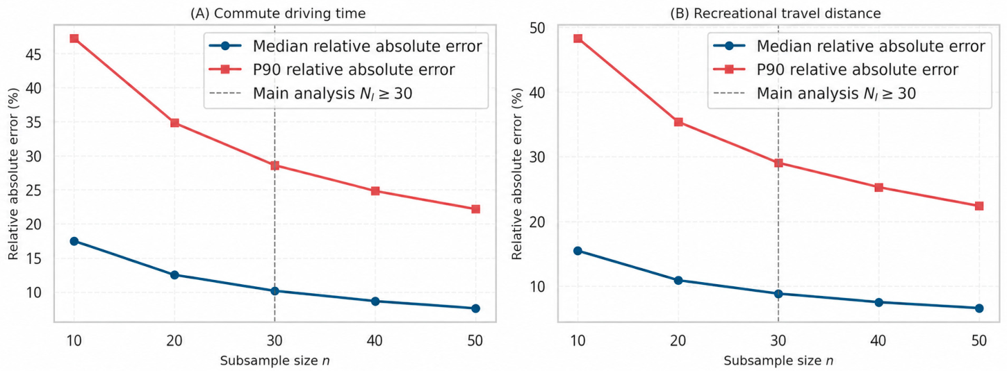
The main analysis retained grids with . This threshold balanced the stability of within-grid median estimates against spatial coverage, as assessed through repeated subsampling of grids with large sample sizes. The full reliability procedure and results are reported in Appendix B.1 (Figure A1), and a stricter threshold was examined in the sensitivity analysis.
2.4.2. Grid-Level Commuting and Recreational Mobility Costs
was the grid median of weekday home-to-work driving time derived from the Baidu Maps Web Service APIs under the temporal settings described in Section 2.2.4. Measured in minutes, it represented the grid-level route-based weekday commuting cost. Driving time was selected because, for repeated and destination-fixed commuting, temporal impedance represents travel cost more directly than home–work distance alone and incorporates network conditions and congestion. Transit time was not retained because, without observed travel mode, an API-derived public-transport itinerary does not necessarily represent realised commuting cost. Its access, waiting, transfer, and route-indirectness components may further weaken its correspondence with the cost actually experienced, while high public-transport impedance may induce mode substitution [20,30]. Consistent with these limitations, the preceding individual-level study [29] found weak coverage of the low-cost range under transit-time measurement.
was the grid median of the individual-level mean weekend recreational mobility costs defined in Section 2.2.4. The main specification used route-based recreational distance in kilometres, consistent with the principal recreational-cost measure used in the preceding individual-level study [29]. For discretionary recreational travel, distance represents both spatial separation and the realised spatial range of activity and was therefore used as the principal recreational indicator. Recreational driving time, which captures temporal impedance under road-network and traffic conditions, was examined as an alternative Stage 1 specification in the sensitivity analysis reported in Section 2.6 and Appendix B.
Stage 1 modelled on the log scale as a smooth function of , with fitted values subsequently back-transformed to the original recreational-distance scale for presentation and coordinate construction. In Stage 2, and were z-standardised together with and before calculating distance correlation, so that differences in measurement scale did not dominate the Euclidean distances. In Stage 3, and entered the coordinate construction on their original scales, with deviations from the fitted reference point standardised using robust scale parameters.
2.4.3. Employment-Centre Proximity and Recreational Opportunity
The opportunity structure for residential grid was defined by , representing employment-centre proximity and cumulative recreational opportunity, respectively. The two components are described below in the order of their construction.
Cumulative recreational opportunity. Recreational opportunity was represented by a behaviourally revealed Hansen-type potential accessibility index combining destination attractiveness and travel impedance [31]. Following Verma and Ukkusuri [32], the impedance-decay parameter was estimated from observed local travel behaviour rather than imposed a priori, because accessibility estimates are sensitive to the assumed rate of distance decay. The technical details of impedance-decay estimation are reported in Appendix C.1.
For residential grid and recreational destination , denoted the number of visits from residents of grid to destination , and denoted total visits to destination . To reduce mechanical overlap between a grid’s own recreational behaviour and its opportunity score, destination attractiveness was defined using the leave-one-origin-out term .
Let denote the set of recreational destinations observed among residents of grid . Cumulative recreational opportunity for residential grid was then calculated as
denoted the mean route-based driving distance associated with visits from residents of grid to recreational destination . The detailed construction of is reported in Appendix C.1.
Although the index was constructed from observed visits rather than exhaustive routing to every possible destination, it combines revealed destination attractiveness with empirically observed route costs and therefore provides a residence-based representation of recreational opportunity. It should be interpreted as opportunity within the empirically observed destination system rather than as exhaustive potential accessibility. The resulting measure was retained on its original, untransformed scale, such that .
Employment-centre identification. To construct the employment-side component of the opportunity structure, employment counts were aggregated to the 1 km grid. Employment-centre cells were then identified using a local log-density peak procedure based on Yan et al. [33]. This local approach was chosen because the objective was to identify relative employment peaks within their surrounding context rather than only globally high-value clusters. The local-regression specification, peak-identification criteria, patch-construction rules, and bandwidth settings are reported in Appendix C.2.
Employment-centre proximity. After employment-centre patches had been identified, the mean travel time between residential grid and employment-centre patch was defined as
Here, was the Baidu Maps Web Service APIs-derived weekday peak-hour driving time for the observed residence–workplace pair of commuter , who resided in grid and worked in a grid cell belonging to an employment-centre patch , and was the number of such commuters in the analytical sample.
Let denote the set of employment-centre patches represented among commuters residing in grid . Employment-centre proximity was then defined as
therefore represented the shortest observed mean commuting time from residential grid to an employment-centre patch represented among its commuters. Lower values indicated greater proximity to the employment-centre system, whereas higher values indicated lower proximity.
Because was defined as the minimum across candidate employment-centre patches, the distribution of candidate-patch counts is reported in Section 3.1.
Stages 2 and 3 used a common complete-case sample of grids with and finite values of , , , and .
2.4.4. Measurement Bases and Analytical Comparability
The cost and opportunity structures were operationalised using a parallel measurement scheme: the employment-related dimensions and were time-based, whereas the recreation-related dimensions were represented by realised route distance () and a distance-decayed opportunity index (). Because the four variables capture distinct constructs, their raw values were neither expected nor required to be directly commensurate. For the cross-structure analyses, Stage 2 z-standardised each variable before calculating distance correlation, while Stage 3 standardised variable-specific deviations before constructing the signed coordinates. The analyses therefore compared relative positions in the two structures rather than raw magnitudes expressed in different units.
2.5. Three-Stage Assessment of the Grid-Level Commuting–Recreation Relationship and Opportunity–Cost Structural Correspondence
Following the framework established in Section 2.3, the analysis proceeded in three stages: Stage 1 examined whether the individual-level U-shaped relationship had a residential-grid counterpart; Stage 2 assessed general dependence between the opportunity and cost structures; and Stage 3 evaluated whether the two structures exhibited the hypothesised curve-based correspondence.
2.5.1. Estimation of the Grid-Level Commuting–Recreation Cost Relationship
Stage 1 estimated
GAM was used to estimate the nonlinear relationship without imposing the fixed parabolic shape and symmetry of a quadratic specification. The GAM implementation and smoothing-parameter selection are detailed in Appendix D.1.
An approximate 95% pointwise confidence band was reported for the fitted smooth. Because the analysis covered the full analytical set of valid residential grids rather than a probability sample, the band was interpreted only as indicating model-based uncertainty in the estimated curve conditional on the observed data and fitted specification, not as uncertainty arising from sampling a broader population.
For presentation and subsequent coordinate construction, fitted values and confidence limits were exponentiated to the original recreational-distance scale. The back-transformed fitted curve was defined as
The valley was identified on the back-transformed curve so that was expressed on the same original distance scale as :
The resulting served as the cost-structure reference for Stage 3. The numerical evaluation used to identify the fitted valley is detailed in Appendix D.1.
2.5.2. Assessment of Multivariate Dependence Between Opportunity and Cost Structures
Stage 2 assessed the overall dependence between the opportunity and cost structures using distance correlation, which can detect general forms of dependence between multivariate vectors, including nonlinear dependence. For residential grid , the opportunity and cost structures were represented by and , respectively.
Using the complete-case grid set defined in Section 2.4.3, each variable was standardised to zero mean and unit variance to prevent differences in measurement scale from dominating the within-structure Euclidean distances. The calculation of sample distance correlation is detailed in Appendix D.2.
To assess whether the observed dependence exceeded that expected under unconstrained random reassignment across grids, the paired cost vectors were reassigned as intact units across residential grids, while the paired opportunity vectors remained fixed. Thus, the within-pair relationships between and , and between and , were preserved, whereas the grid-specific correspondence between the opportunity and cost structures was removed. The permutation count and Monte Carlo p-value calculation are reported in Appendix D.2.
Because unrestricted reassignment did not preserve the spatial dependence structure of the cost vectors across grids, the resulting -value was interpreted as a benchmark against unconstrained random reassignment rather than as a spatially robust test of independence.
2.5.3. Assessment of Curve-Based Correspondence Between Opportunity and Cost Structures
Stage 3 tested the more specific hypothesis that residential grids occupied corresponding positions along the fitted employment–recreation opportunity curve and the fitted commuting–recreation cost curve. This involved identifying a reference point on each curve, converting each grid’s position relative to those reference points into signed coordinates, and assessing the correspondence between the two coordinates.
(1) Estimation of the employment–recreation opportunity relationship
Using the same grid set as Section 2.5.2, the nonlinear relationship between employment-centre proximity and recreational opportunity was estimated as
where denotes the smooth function relating employment-centre proximity to recreational opportunity . The model used the same penalised cubic-spline specification as in Stage 1. Because was analysed on its original, untransformed cumulative-opportunity scale, no outcome transformation or back-transformation was applied.
The fitted maximum of the opportunity curve was identified within the observed support of :
The numerical evaluation used to identify the fitted maximum is reported in Appendix D.1.
Here, denotes the employment-centre proximity at which fitted recreational opportunity was maximised, and is the corresponding fitted opportunity level. The fitted maximum was used as an empirically derived reference point for constructing the signed opportunity coordinate. This construction did not assume a symmetric inverted-U relationship; rather, it distinguished grids located on either side of the fitted maximum and quantified their scaled deviation from that reference.
(2) Construction of signed coordinates
The fitted opportunity and cost relationships were translated into one-dimensional coordinates retaining both the side of the empirically derived fitted maximum or valley and the magnitude of scaled deviation from the corresponding reference point. The opportunity-side reference was obtained from the fitted opportunity curve, while the cost-side reference was the valley identified from the Stage 1 commuting–recreation curve.
Because the horizontal and vertical components were measured in different units and had different dispersions, each deviation was standardised before being combined into a single coordinate. For , robust scales were defined as , where MAD denotes the median absolute deviation. When MAD was zero, , where IQR denotes the interquartile range; when both MAD and IQR were zero. These robust scale factors standardised the horizontal and vertical deviations to comparable, unit-free scales before they were combined into a single coordinate.
The side indicators were defined as
The main signed coordinates were
Intuitively, each signed coordinate represents both the side of the fitted reference point on which a grid lies and its scaled displacement from that reference configuration (illustrated for the valley-based cost coordinate in Figure 4). For , the sign indicates whether lies below or above , while the absolute magnitude is the Euclidean combination of the scaled horizontal deviation from and any upward deviation of recreational cost from the fitted minimum . Values of at or below therefore make no contribution to the vertical deviation term. The opportunity-side coordinate is constructed analogously, except that the vertical direction is reversed: its vertical term captures any downward deviation of recreational opportunity from the fitted maximum . Values of at or above therefore make no contribution to this term.
Figure 4.
Schematic illustration of the signed-coordinate construction. The figure illustrates the valley-based cost coordinate . The peak-based opportunity coordinate is constructed analogously, except that the adverse vertical deviation is defined as the shortfall below , rather than the excess above .
The one-sided vertical terms were used to encode deviations in the direction treated as adverse in the main specification; deviations in the opposite direction were set to zero. Accordingly, and should be interpreted as empirical positional indices relative to their respective fitted reference configurations, rather than as measures premised on fully developed or symmetric U-shaped and inverted-U structures. Non-truncated alternatives were examined in Section 2.6.
(3) Coordinate-based assessment of opportunity–cost correspondence
The coordinate model assessed whether residential grids occupied corresponding positions in the opportunity and cost configurations:
OLS was used as a descriptive specification to summarise the approximate alignment between the two signed coordinates, which represented the positions of grids relative to their respective empirically fitted reference points. Distance correlation in Section 2.5.2 assessed whether the two multivariate structures were generally dependent; the coordinate model assessed the more specific hypothesis that residential grids occupied corresponding relative positions in the opportunity and cost configurations, as represented by the direction and magnitude of their signed displacement from the respective fitted reference points.
Three descriptive benchmarks were fitted on the same complete-case grid set:
The first two benchmarks related separately to and , while the third represented their additive joint relationship without encoding the fitted opportunity-curve geometry. The single-variable benchmarks showed how much descriptive fit was obtained from either opportunity dimension alone. The additive model retained both dimensions without imposing the fitted-curve geometry and therefore provided a benchmark for the information retained when was reduced to the single theory-informed coordinate . It was not treated as an alternative test of curve-based correspondence. These models were descriptive comparators rather than formal tests of the superiority of . Models were compared using adjusted , with standardised coefficients reported for unit-free comparison. Because all models were fitted to the same dependent variable and complete-case grid set, adjusted provided a directly comparable in-sample measure of descriptive fit.
Because the analysis covered the full analytical set of residential grids satisfying the study’s validity and complete-case criteria, the models were interpreted descriptively for those grids. Reporting therefore focused on descriptive coefficients, adjusted , and model diagnostics rather than formal superpopulation inference.
2.6. Sensitivity Analysis Specifications
Sensitivity analyses were organised by analytical component and examined whether the relevant findings depended on alternative choices concerning recreational-cost measurement, spatial resolution, minimum within-grid sample size, centre-identification scale, and coordinate construction.
Stage 1 was re-estimated using recreational driving time in place of recreational distance, 500 m and 2 km residential grids in place of the 1 km main resolution, and alternative minimum within-grid sample-size thresholds of and , compared with the baseline . These analyses assessed whether the fitted cost-side relationship and valley depended on representing recreational cost by distance rather than time, and whether the results depended on spatial resolution or the minimum within-grid sample size. The scope and implementation of these specifications are detailed in Appendix E.1.
For Stages 2 and 3, the sensitivity of the results to the employment-centre identification scale was assessed using 3000 m and 7000 m search bandwidths, with 5000 m retained as the baseline. Employment-centre proximity was reconstructed under each specification, and the opportunity-curve, distance-correlation, coordinate, and benchmark analyses were repeated on the common complete-case sample available under all three bandwidths. Comparisons focused on the identified employment-centre structure, the opportunity-side reference point, multivariate dependence, and the strength and relative descriptive performance of the curve-based correspondence.
Stage 3 was additionally repeated using coordinate definitions without one-sided truncation of vertical deviations to assess whether the results depended on retaining only deviations in the direction treated as adverse in the main specification. The alternative coordinate definitions and implementation procedure are detailed in Appendix E.2.
3. Results
3.1. Analytical Sample and Spatial Distributions of the Core Variables
A total of 971 residential grids satisfying the Stage 1 validity criteria were included in the analysis. Requiring finite values for all four core variables yielded 970 complete-case grids for Stages 2 and 3; one grid was excluded because no valid employment-centre route-time connection was available from which to construct . Because was operationalised as the minimum observed mean commuting time across candidate employment-centre patches, the number of candidate patches represented for each residential grid was also examined. This number had a median of 32 and a fifth percentile of 5, indicating that was generally calculated from multiple observed employment-centre connections rather than from a single candidate patch.
Table 1 summarises the distributions of the four core variables. Their median values were 18.27 min for commuting cost , 9.30 km for recreational mobility cost , 8.63 min for employment-centre proximity , and 137,281.84 for recreational opportunity on its original, untransformed scale.
Table 1.
Descriptive statistics of the four core grid-level variables.
Figure 5 reveals pronounced spatial heterogeneity across all four variables. Visual comparison also suggests some correspondence between the spatial patterns of the cost variables and and those of the opportunity-side variables and , although the patterns are neither uniform nor fully coincident. This map-based comparison is descriptive and does not establish correspondence between the two bivariate structures, which is examined formally in Stages 2 and 3.
Figure 5.
Spatial distributions of commuting cost , recreational mobility cost , employment-centre proximity , and recreational opportunity across 1 km residential grids. Panels (a,b) use the Stage 1 analytical sample; panels (c,d) use the complete-case sample for Stages 2 and 3. Colour scales are variable-specific and are not directly comparable across panels. Any apparent co-location of similarly shaded areas is descriptive only and should not be interpreted as statistical evidence of association; cross-structure dependence and curve-based correspondence are assessed separately in Stages 2 and 3, respectively.
3.2. Grid-Level Commuting–Recreation Cost Relationship
At the residential-grid level, a U-shaped pattern emerged between commuting driving time and recreational travel distance across the 971 valid 1 km grids (Figure 6). The smooth term had an effective degrees of freedom of 4.23, and the model explained 7.76% of the deviance. The effective degrees of freedom remained well below the complexity permitted by the 20-basis-function specification, indicating that the fitted smooth was not constrained by the selected basis dimension. The modest explained deviance indicates that the fitted relationship captured only a limited proportion of the overall cross-grid variation in recreational distance.
Figure 6.
Grid-level relationship between commuting driving time and recreational travel distance .
The back-transformed fitted curve declined as commuting time increased to min, where the minimum fitted recreational distance was 8.01 km, and then increased over the remainder of the main data-support range. Within the 5th–95th percentile range of (6.7–29.1 min), the fitted recreational distance declined by 16.6%, from 9.60 km to 8.01 km, and then increased by 26.0% to 10.09 km. The estimated valley remained stable across the alternative recreational-cost measure, spatial resolutions, and grid-validity thresholds, ranging from 15.69 to 16.96 min (Appendix B, Figure A2 and Table A3).
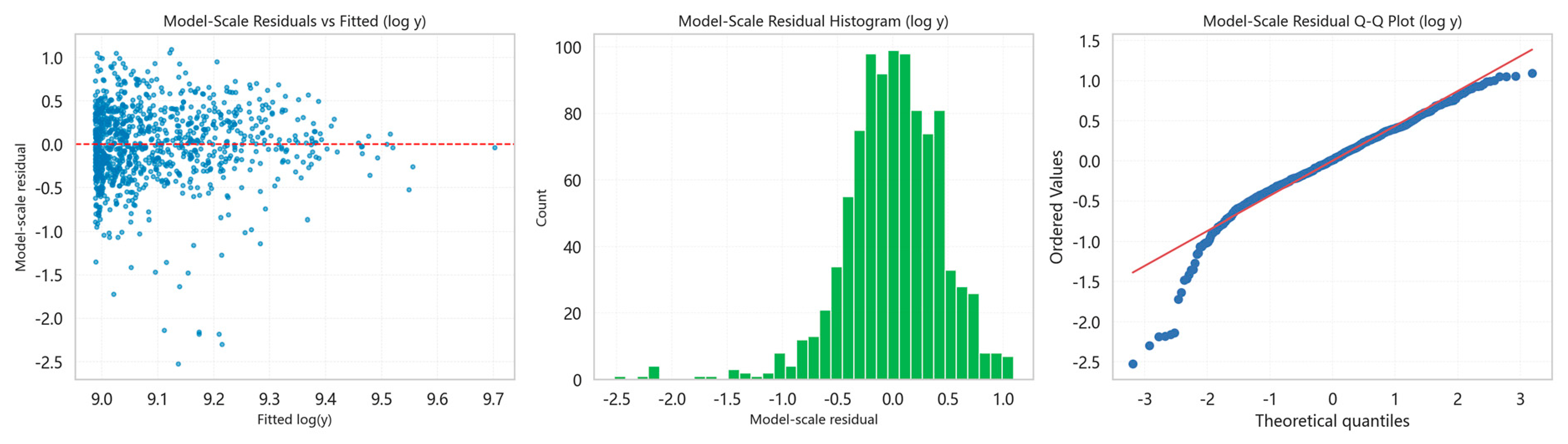
The approximate 95% pointwise confidence band was relatively narrow across the densely populated central range of commuting times but widened in the sparsely populated upper tail. Only 37 grids (3.8%) had commuting times above 30 min; therefore, estimates in this sparsely supported range were interpreted cautiously and were not used as the primary basis for evaluating the overall U-shaped pattern. Residual diagnostics revealed no pronounced remaining curvature but showed heteroscedasticity and a heavier-than-normal lower tail (Appendix B, Figure A3).
3.3. Multivariate Dependence Between Opportunity and Cost Structures
The distance correlation between the opportunity structure and the cost structure was across the 970 complete-case residential grids. All 9999 statistics generated by unrestricted reassignment of the intact cost vectors across grids were below 0.11, far below the observed value, yielding a one-sided Monte Carlo (Figure 7).
Figure 7.
Permutation distribution of the distance correlation between the opportunity structure and the cost structure .
The observed dependence was therefore substantially stronger than that generated by the unconstrained random-reassignment benchmark. Because unrestricted reassignment did not preserve the spatial dependence structure of the cost vectors, this -value was interpreted as a non-spatial benchmark rather than as a spatially robust test of independence. The result supports general multivariate dependence relative to that benchmark but does not identify its functional form or establish the hypothesised curve-based correspondence, which are examined in Section 3.4 and Section 3.5.
3.4. Employment–Recreation Opportunity Curve
Across the 970 complete-case residential grids, the fitted GAM indicated an inverted U-shaped relationship between employment-centre proximity and recreational opportunity (Figure 8). The smooth term had an EDF of 5.62, and the model explained 24.65% of the deviance. The widening confidence band towards higher values of reflects declining observational support in this range, which increases uncertainty in the fitted curve.
Figure 8.
Relationship between employment-centre proximity and recreational opportunity .
Within the 5th–95th percentile range of (3.1–22.2 min), fitted recreational opportunity increased from 85,376 to a maximum of at min and then declined to 304,374. The fitted maximum lay within the well-supported interior of the observed range and was used as the opportunity-side reference point for the coordinate construction in Section 3.5.
3.5. Curve-Based Opportunity–Cost Correspondence
The signed opportunity coordinate was positively related to the signed cost coordinate across the 970 complete-case residential grids (Figure 9; Table 2). The standardised coefficient was 0.364, and the model had an adjusted of 0.132, indicating a positive but partial correspondence between grids’ relative positions in the fitted opportunity and cost configurations.
Figure 9.
Coordinate-based correspondence between opportunity and cost structures.
Table 2.
Descriptive comparison of the coordinate model and benchmark specifications.
The coordinate model provided a better descriptive fit than either opportunity dimension considered separately. The adjusted values were 0.108 for the -only model and 0.100 for the -only model, compared with 0.132 for the coordinate model. This indicates that neither employment-centre proximity nor recreational opportunity alone fully captured the observed correspondence.
The additive model produced a higher adjusted of 0.165. Its standardised coefficients were 0.265 for and 0.248 for , indicating that both dimensions retained descriptive associations with when entered jointly. The coordinate model nevertheless retained most of the available descriptive fit of the additive specification while reducing the two opportunity dimensions to a single coordinate that explicitly represented the fitted curve geometry.
Overall, the results support a positive but limited curve-based correspondence between the opportunity and cost structures. Residential grids tended to occupy corresponding positions in the two configurations, as reflected in the direction and magnitude of their signed displacement from the respective fitted reference points, although substantial cross-grid variation remained unexplained. This correspondence is consistent with the spatial hypothesis.
3.6. Sensitivity Analyses
Sensitivity analyses examined alternative outcome measures, spatial resolutions, grid-validity thresholds, employment-centre bandwidths, and coordinate definitions.
The Stage 1 U-shaped relationship was retained across all alternative specifications. Replacing recreational distance with driving time retained the U-shaped form and shifted the valley by only 0.92 min, from 16.61 to 15.69 min. Across the full set of alternative specifications, the fitted valley ranged from 15.69 to 16.96 min, and explained deviance ranged from 7.13% to 8.48% (Appendix B, Figure A2; Appendix B, Table A3).
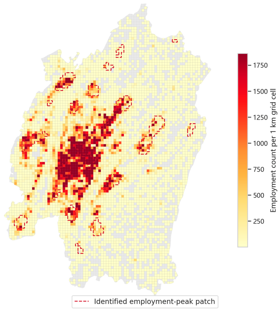
Employment-centre bandwidth sensitivity was assessed using 3000 m and 7000 m alternatives to the 5000 m baseline. Comparisons used the common set of 963 grids with complete values under all three specifications. The fitted opportunity-side reference remained stable (–13.7 min), while distance correlation varied only from 0.498 to 0.518, with in all cases under the unconstrained random-reassignment benchmark. The coordinate relationship also remained positive but weakened under the 7000 m specification: the standardised coefficient declined from 0.364 to 0.226, and adjusted from 0.132 to 0.050 (Appendix B, Table A4). Under this specification, the coordinate model no longer outperformed the recreational-opportunity-only benchmark. A post hoc visual inspection indicated that several major high-employment concentrations were not delineated as local peak patches under the 7000 m specification (Appendix B, Figure A4).
Using non-truncated coordinates produced results close to the baseline specification, with a standardised coefficient of 0.349 and an adjusted of 0.121 (Appendix B, Table A5).
Overall, the U-shaped relationship and general multivariate dependence were stable, and the coordinate relationship remained positive. The weaker correspondence at 7000 m coincided with incomplete delineation of major employment concentrations and was therefore interpreted cautiously rather than as direct evidence against the curve-based correspondence.
4. Discussion
4.1. Spatial Manifestation of the U-Shaped Relationship and Opportunity–Cost Correspondence
The results extend the preceding individual-level finding [29] in two respects. First, they show that the U-shaped commuting–recreation relationship is not confined to individual-level variation but also has a residential-grid manifestation. Second, they relate this spatial manifestation to the employment–recreation opportunity structure, thereby moving the analysis beyond a bivariate mobility-cost relationship. The evidence therefore shifts from documenting an empirical commuting–recreation association to assessing whether that association has a spatial-structural basis.
4.1.1. A Residential-Grid Manifestation of the U-Shaped Relationship
RQ1 asked whether the previously identified individual-level U-shaped relationship could also be observed at the spatial level. The grid-level analysis identified a corresponding U-shaped pattern, with recreational mobility cost reaching its fitted minimum at an intermediate commuting cost.
The relationship and the location of its fitted minimum remained stable across alternative recreational-cost measures, spatial resolutions, and grid-validity thresholds. These results therefore provide an affirmative answer to RQ1: the individual-level U-shaped relationship has a corresponding spatial manifestation. This conclusion applies primarily to the well-supported commuting-cost range, because estimates in the sparse upper tail remain less certain.
4.1.2. Correspondence Between Opportunity and Cost Structures
RQ2 asked whether the grid-level commuting–recreation relationship corresponded to the spatial relationship between employment-centre proximity and recreational opportunity. Distance correlation first showed that the two original bivariate structures were generally dependent relative to the random-reassignment benchmark, indicating that their association was not created solely by the subsequent coordinate construction. The signed-coordinate model then identified a positive correspondence between grids’ relative positions in the two fitted configurations.
This correspondence was positive but partial. The standardised coefficient was 0.364, while the adjusted of 0.132, and the dispersion around the fitted line indicate that the relationship represents an average cross-grid tendency rather than a strong prediction of individual grid positions. The coordinate model nevertheless provided a better descriptive fit than either employment-centre proximity or recreational opportunity considered separately, and its adjusted was only 0.033 lower than that of the additive benchmark. This suggests that the theory-informed coordinate retained most of the descriptive fit available from the two opportunity dimensions while explicitly representing their fitted-curve geometry.
The positive coordinate relationship was retained across the examined specifications. Its weaker magnitude under the 7000 m bandwidth coincided with incomplete delineation of several major employment concentrations and was therefore interpreted cautiously rather than as direct evidence against the correspondence.
RQ2 therefore receives an affirmative but bounded answer: the grid-level commuting–recreation relationship corresponds to the spatial relationship between employment-centre proximity and recreational opportunity, but the identified correspondence captures only part of the cross-grid variation in the cost structure. Together with the spatial manifestation of the U-shaped relationship identified in Section 4.1.1, this result provides spatial evidence consistent with the jobs–housing–recreation interpretation proposed in the preceding individual-level study [29].
4.2. Spatial-Structural Interpretation of the Commuting–Recreation Relationship
4.2.1. Spatial Configurations Along the U-Shaped Relationship
The aggregate correspondence established in Section 4.1 does not by itself reveal how it is spatially constituted. A theory-guided reading of Figure 5 was therefore used to characterise the residential-location configurations associated with different segments of the U-shaped relationship.
The mapped distributions suggest three recurring configurations. First, some low-commuting-cost grids are centrally located and combine short commutes with higher recreational opportunity and lower recreational mobility cost. Second, other low-commuting-cost grids are located in peripheral areas where proximity to secondary employment centres permits short observed commutes, but recreational opportunity remains weaker and recreational mobility cost higher. Third, many high-commuting-cost grids are peripheral locations characterised by both longer travel times to employment centres and weaker recreational opportunity. Grids around the fitted minimum more often occupy locations where employment-centre proximity and recreational opportunity are comparatively well balanced.
These configurations clarify why the lower end of the commuting-cost distribution does not represent a homogeneous spatial condition. The coexistence of centrally advantaged locations and peripheral, employment-proximate but recreation-poor locations is consistent with the elevated fitted recreational costs on the left-hand side of the curve, whereas the rising right-hand side is consistent with compounded employment and recreational disadvantage in more peripheral locations. The U-shaped relationship is therefore better interpreted not as a simple commuting–recreation trade-off, but as a spatial manifestation of the uneven alignment of polycentric employment and spatially distributed recreational opportunities across residential locations. This interpretation also provides a spatial basis for differentiated coordination of jobs, housing, and recreational provision.
4.2.2. Why Opportunity–Cost Correspondence Remains Partial
The measured opportunity structure describes the spatial conditions associated with residential locations, whereas commuting and recreational mobility costs reflect how residents actually engage with those conditions. The modest explanatory power of the signed-coordinate model is therefore not inconsistent with a spatial-structural interpretation; rather, it indicates that spatial opportunity constrains and enables mobility without determining it mechanically.
One source of divergence is population–opportunity matching. Employment centres contain jobs that differ in their relevance to workers with different occupations and skills, while recreational destinations vary in their relevance to different demographic groups, household types, and preferences. Residential locations with similar measured employment-centre proximity or recreational opportunity may therefore provide substantially different effective opportunities to their residents.
A second source is residential sorting and behavioural adaptation. Households select residential and employment locations under multiple constraints, including housing cost, household composition, school access, and transport availability, rather than solely to minimise commuting or recreational travel. Residents may also respond to the same opportunity environment through different destination choices, travel modes, and activity frequencies [34]. These processes influence both the spatial conditions to which residents are exposed and the extent to which those conditions are translated into realised mobility costs.
The observed correspondence should therefore be understood as a structural tendency rather than a deterministic mapping. The jobs–housing–recreation configuration provides an important spatial context for commuting and recreational mobility, but realised outcomes also depend on population matching, household sorting, behavioural choice, and transport conditions.
4.2.3. Urban-Form Context and Broader Relevance
The broader relevance of the Chongqing findings lies not in expecting the same U-shaped relationship to recur across cities, but in the more general spatial proposition that commuting and recreational mobility conditions are jointly related to how employment and recreational opportunities are organised around residential locations. Urban form matters because it shapes the spatial alignment of these two opportunity systems. Where they exhibit broadly similar spatial gradients, commuting and recreational mobility costs may vary in a relatively consistent direction; where their distributions are spatially differentiated, residential locations may combine employment access and recreational opportunity in more varied ways, allowing nonlinear relationships to emerge. The U-shaped pattern observed in Chongqing is one possible expression of this more general spatial relationship rather than its necessary form.
Different metropolitan structures provide contrasting settings for this proposition. London contains multiple functional communities within an increasingly polycentric structure [35], whereas Los Angeles exhibits a highly decentralised employment pattern with numerous subcentres and substantial employment outside them [36]. Chongqing combines polycentric development with mountainous terrain and major river barriers that strongly constrain the spatial organisation and connectivity of urban activities. These differences do not imply predetermined commuting–recreation relationships but indicate that the form and strength of such relationships may vary with the way employment and recreational opportunities are spatially aligned in different urban contexts. Cross-city analysis is therefore needed to determine which aspects of the Chongqing pattern are transferable and which depend on its particular spatial configuration.
4.3. Advancing Commuting–Recreation Spatial-Performance Research
The present findings establish a spatial correspondence between commuting–recreation mobility costs and the measured employment–recreation opportunity structure, but also show that this correspondence accounts for only part of the observed cross-grid variation. For planning, this supports a diagnostic use of the framework: spatial-structure evaluation can identify locations where employment and recreational-opportunity conditions are jointly associated with unfavourable mobility outcomes, rather than assessing commuting or recreational performance in isolation. Such diagnosis can distinguish locations facing disadvantages in both domains from those characterised primarily by an employment- or recreation-related shortfall, providing a basis for differentiated rather than uniform intervention.
The more important next step is to determine whether the remaining variation reflects the limited spatial relevance of the measured opportunity structure or the inability of general opportunity measures to represent population-specific access to jobs and recreational destinations. Future research should distinguish three analytical layers: general spatial opportunity, population-specific effective opportunity, and realised mobility cost. General opportunity measures describe the employment and recreational resources associated with a residential location. Population-specific effective opportunity measures would additionally account for whether those resources are relevant and accessible to particular groups. Comparing the explanatory contribution of general and population-specific opportunity measures would show how much additional variation in commuting and recreational mobility costs is explained by population–employment and population–recreation matching.
A substantial increase in explanatory power would strengthen the evidence that population–opportunity matching helps account for the relationship between jobs–housing–recreation structure and realised mobility costs, and would provide a stronger basis for identifying which employment and recreational opportunities should be improved for particular population groups and locations. Limited improvement would instead suggest that household locational choices, individual preferences, transport conditions, measurement limitations, or other factors less directly amenable to spatial intervention account for much of the remaining variation. This comparison would allow commuting–recreation spatial-performance research to progress from joint spatial-performance diagnosis towards evaluating and designing more targeted interventions, while clarifying the extent to which commuting and recreational performance can realistically be improved through coordinated spatial planning [37].
4.4. Limitations
Several limitations define the scope of the conclusions. First, the observed correspondence does not isolate the contribution of the measured opportunity structure. Realised mobility costs may also reflect population–employment and population–recreation matching, household locational choices, transport conditions, and destination choice. Because the opportunity measures represent general employment and recreational opportunities rather than population-specific effective opportunities, the findings support a spatial-structural interpretation but do not determine how much of the observed cost structure is accounted for by the measured opportunity structure.
Second, recreational distance and travel time measure realised recreational mobility costs, not the full utility of recreation. Longer trips may reflect higher destination quality, novelty, or better alignment with individual or household preferences, while shorter trips do not always imply greater utility. Future research should incorporate destination quality, activity type, satisfaction, and visit frequency to assess recreational utility more fully.
Third, the temporal and urban-context scope of the evidence is limited. The data cover a single observation period in Chongqing and do not establish whether the relationship remains stable across seasons or years. Chongqing’s mountainous terrain, clustered urban form, and differentiated spatial distribution of employment centres and recreational opportunities may affect the shape of the U-shaped relationship, the associated residential-location configurations, and the strength of the opportunity–cost correspondence. The analytical framework can be tested in other contexts, but the specific empirical results require multi-period and multi-city validation.
5. Conclusions
Although commuting and recreational mobility are theoretically related, their empirical relationship has rarely been examined directly. A preceding study in Chongqing reported a U-shaped relationship between commuting and recreational mobility costs at the individual level and proposed that it might reflect how employment and recreational opportunities are combined across residential locations within the jobs–housing–recreation spatial structure. That interpretation, however, had not been tested at the spatial level.
The present study addresses this gap by showing that a corresponding U-shaped relationship emerges across residential grids and that the commuting–recreation cost structure exhibits general multivariate dependence and a positive but partial curve-based correspondence with the employment–recreation opportunity structure. The mapped distributions further suggest that the two sides of the U-shaped relationship are associated with different combinations of employment-centre proximity and recreational opportunity. Together, these findings provide spatial evidence consistent with the interpretation that the U-shaped relationship partly reflects the uneven alignment of polycentric employment and spatially distributed recreational opportunities across residential locations. These findings suggest that commuting and recreational mobility may benefit from being considered jointly when assessing jobs–housing–recreation spatial performance and exploring opportunities for coordinated improvement across both domains.
The positive correspondence nevertheless captured only part of the cross-grid variation in the cost structure. Future research should therefore distinguish general spatial opportunity, population-specific effective opportunity, and realised mobility cost, and examine whether incorporating population–employment and population–recreation matching increases the explanatory contribution of the opportunity structure. The extent of such improvement would clarify both the explanatory reach of the spatial-structural interpretation and the realistic scope for improving commuting and recreational performance jointly through coordinated spatial planning.
These conclusions remain bounded in three respects. The observed correspondence does not isolate how much of the cost structure is accounted for by the measured opportunity structure, because realised mobility costs also reflect population matching, household locational choices, transport conditions, and destination choice. Recreational distance and travel time measure realised recreational mobility costs rather than the full utility derived from recreational activity. Finally, the evidence is drawn from a single five-week observation period in Chongqing; whether the U-shaped relationship, its associated residential configurations, and the strength of opportunity–cost correspondence remain stable across time and other urban contexts requires multi-period and multi-city validation.
Author Contributions
Conceptualisation, C.F.; Methodology, C.F.; Software, C.F.; Formal analysis, C.W. and C.F.; Investigation, C.F.; Data curation, C.F.; Writing—original draft preparation, C.F.; Visualisation, C.W.; Writing—review and editing, Y.L., G.Y. and C.F.; Funding acquisition, Y.L. and C.F.; Supervision, Y.L. All authors have read and agreed to the published version of the manuscript.
Funding
This research was funded by the National Natural Science Foundation of China (52408054 and 52478042), and the Key Project of Higher Education Teaching Reform Research in Chongqing (252018).
Data Availability Statement
The individual-level location-based services (LBS) data used in this study were obtained from a commercial provider under licence and are not publicly available due to commercial, contractual, privacy, and ethical restrictions. The authors are not permitted to deposit or redistribute the raw data. The study’s analytical workflow and variable construction procedures are described in Section 2.
Acknowledgments
During the preparation of this manuscript, the first author used ChatGPT (OpenAI, San Francisco, CA, USA; https://chatgpt.com/; accessed between March and July 2026) to assist with language polishing and clarity improvement, and Cursor (Anysphere Inc., San Francisco, CA, USA; https://www.cursor.com/; accessed between March and July 2026) to support code development and debugging. All scientific content, methodological design, analyses, interpretations, and conclusions were developed by the authors, who take full responsibility for the content of this publication.
Conflicts of Interest
The authors declare no conflicts of interest.
Abbreviations
The following abbreviations are used in this manuscript:
| LBS | location-based services |
| GAM | generalised additive model |
| EDF | effective degrees of freedom |
| dCor | distance correlation |
Appendix A. Recreational AOI Definition and Multiplicity
Table A1.
AOI categories included to identify weekend recreational visits.
Table A2.
Distribution of distinct recreational AOIs visited per person-day.
Appendix B. Supplementary Reliability Assessment, Model Diagnostics, and Sensitivity Analyses
Appendix B.1. Subsampling Reliability of Within-Grid Medians
To assess the reliability of within-grid medians at different sample sizes, repeated without-replacement subsampling was conducted using 735 grids with at least 100 valid observations. For each grid and , 500 subsamples were drawn and compared with the median calculated from all valid observations in that grid. Relative absolute errors were summarised by their median and 90th percentile.
At , median relative absolute errors were 10.2% for commuting driving time and 8.9% for recreational travel distance, while the corresponding 90th-percentile errors were 28.6% and 29.0%. Errors declined further at larger sample sizes, but the incremental improvement was smaller. These results support as a pragmatic balance between median stability and spatial coverage rather than as a sharp statistical cutoff.
Figure A1.
Subsampling reliability of within-grid median estimates. Results are based on 735 calibration grids with . Points show the median and 90th-percentile relative absolute errors across 500 subsamples at each sample size; the dashed line marks .
Appendix B.2. Sensitivity of the Grid-Level Commuting–Recreation Relationship
The Stage 1 relationship was re-estimated using an alternative recreational-cost measure, 500 m and 2 km residential grids, and relaxed and stricter within-grid sample-size thresholds. All five alternative specifications retained the U-shaped pattern identified in the primary analysis.
Figure A2.
Sensitivity of the grid-level commuting–recreation relationship. Panels show the alternative recreational-driving-time outcome, 500 m and 2 km residential grids, and the and thresholds.
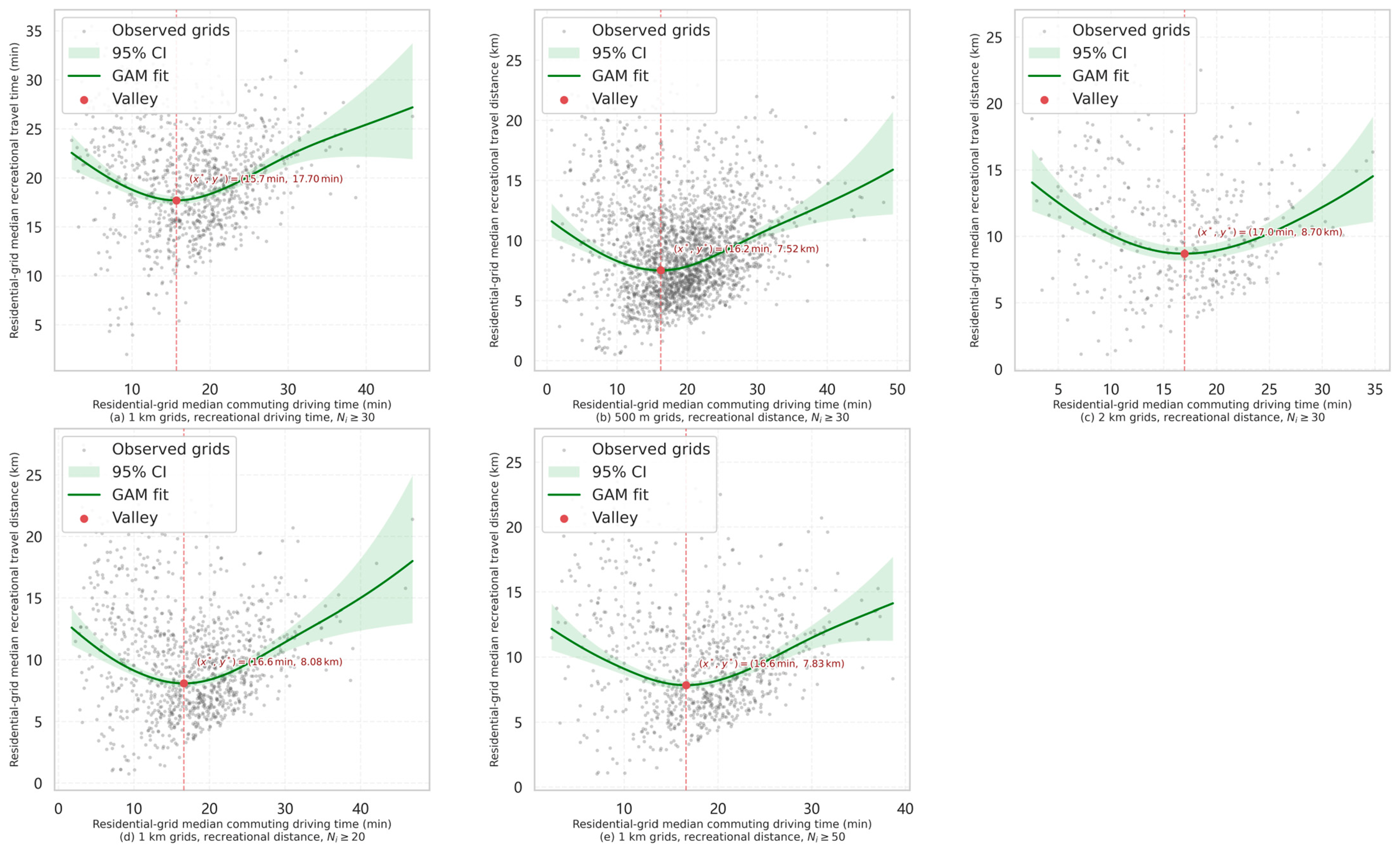
Table A3.
GAM results for the primary and sensitivity specifications of the grid-level commuting–recreation relationship.
Appendix B.3. Model Diagnostics for the Primary Grid-Level GAM
Residual diagnostics were examined for the primary Stage 1 specification to assess whether the fitted functional form left pronounced systematic structure in the residuals. No clear residual curvature was observed, although residual dispersion varied across fitted values and the lower tail departed from normality.
Figure A3.
Residual diagnostics for the primary grid-level GAM. The panels show model-scale residuals against fitted values, the residual distribution, and the normal Q–Q plot. In the residuals-versus-fitted panel, the red dashed horizontal line indicates zero residual; in the normal Q–Q panel, the red solid line represents the normal-reference line.
Appendix B.4. Employment-Centre Bandwidth Sensitivity
Employment-centre bandwidth sensitivity was assessed using 3000 m and 7000 m alternatives to the 5000 m baseline. The opportunity-curve, Stage 2, and Stage 3 comparisons were calculated on the common set of 963 residential grids with complete values under all three bandwidths. Seven of the 970 baseline complete-case grids lacked finite values under at least one alternative bandwidth and were excluded so that all three specifications were compared on an identical sample. The fitted opportunity-side reference location remained highly stable, although the number of identified centre cells and patches varied considerably. General multivariate dependence and the positive direction of curve-based correspondence were retained. Under the 7000 m specification, however, the coordinate model weakened substantially and no longer provided a better descriptive fit than the recreational-opportunity-only benchmark. A post hoc visual inspection indicated that several major high-employment concentrations were not delineated as local peak patches under the 7000 m specification, suggesting that the broader bandwidth produced an incomplete representation of the local employment-centre structure (Figure A4).
Table A4.
Employment-centre bandwidth sensitivity across opportunity-curve, Stage 2, and Stage 3 results.
Figure A4.
Employment-density surface and local employment-peak patches identified using a 7000 m search bandwidth. The dashed outlines denote the identified local peak patches. Several high-employment concentrations were not delineated as local peaks under this broader-bandwidth specification.
Appendix B.5. Sensitivity to Coordinate Construction
The coordinate-based correspondence was further examined using non-truncated structural coordinates. The alternative coordinate definition produced results close to the baseline specification.
Table A5.
Sensitivity of coordinate-based correspondence.
Appendix C. Detailed Construction of the Opportunity-Structure Variables
Appendix C.1. Detailed Estimation and Aggregation Procedures for Cumulative Recreational Opportunity
A negative-exponential decay function, , was fitted to the local empirical recreational-distance distribution. The survival curve was approximated by using Levenberg–Marquardt nonlinear least squares.
For each observed visit, the route distance was measured from the residential grid to which the visit record was assigned to destination , and these distances were averaged across all visit records associated with the same residential-grid–destination pair . Thus, was the observed mean route distance for the pair.
The measure was constructed from observed visit records rather than through exhaustive routing of all possible home-grid–destination combinations.
Appendix C.2. Detailed Employment-Centre Identification Procedure
For each grid cell, an ordinary least-squares regression of on Euclidean centroid-to-centroid distance was fitted using the grid cells within a circular neighbourhood of bandwidth . A grid cell was classified as a local peak when the estimated distance coefficient was negative and . Neighbourhoods containing fewer than five grid cells were excluded to avoid fitting local regressions with too few observations. Contiguous peak grid cells were merged into patches using Queen contiguity, and patches consisting of only one grid cell were removed to reduce sensitivity to isolated peak cells. The main analysis used a 5000 m bandwidth; 3000 m and 7000 m alternatives were examined for scale sensitivity.
Appendix D. Model Estimation and Statistical-Test Implementation
All data processing and statistical analyses were implemented in Python version 3.9.23. GAMs were estimated using the LinearGAM class in pyGAM version 0.10.1. The Stage 3 coordinate and benchmark OLS models were fitted using numpy.linalg.lstsq in NumPy version 1.24.3, whereas the local regressions used for employment-centre identification were fitted using scipy.stats.linregress in SciPy version 1.13.1. Distance-correlation and permutation analyses were implemented directly using NumPy version 1.24.3. Nonlinear least-squares estimation was performed using scipy.optimize.least_squares with the Levenberg–Marquardt algorithm in SciPy version 1.13.1. Spatial data processing was conducted using GeoPandas version 0.14.1, Shapely version 2.0.1, and libpysal version 4.8.1.
Appendix D.1. GAM Implementation and Numerical Identification of Fitted Reference Points
The Stage 1 model was estimated using LinearGAM classs in pyGAM with the default cubic penalised spline basis comprising 20 basis functions. effective complexity controlled through penalisation. The smoothing parameter was selected by GCV from 11 logarithmically spaced values between and , covering a broad range of penalisation strengths. Effective degrees of freedom were inspected to assess whether the fitted smooth approached the complexity permitted by the selected basis dimension.
The curve was plotted together with the observed grid-level data and evaluated at 1000 evenly spaced points over the observed support . The minimum of the back-transformed fitted curve was used to identify the cost-structure reference point .
The Stage 3 employment–recreation opportunity model used the same penalised cubic-spline specification, basis dimension, and smoothing-parameter selection procedure as the Stage 1 model. The fitted opportunity curve was evaluated at 1000 evenly spaced values spanning the observed support of . Its maximum was used to identify the opportunity-side reference point .
Appendix D.2. Distance-Correlation Calculation and Permutation Implementation
Sample distance correlation was calculated from the doubly centred Euclidean distance matrices of the two multivariate structures.
The procedure was repeated times. This number of permutations provides a minimum attainable Monte Carlo p-value of and sufficient resolution for the single omnibus dependence assessment conducted here. The one-sided upper-tail Monte Carlo p-value was calculated as
where denotes the number of permuted statistics at least as large as the observed distance correlation.
Appendix E. Implementation Details for Sensitivity Analyses
Appendix E.1. Scope and Implementation of the Stage 1 Sensitivity Analyses
The Appendix subsampling assessment evaluated the sampling-related stability of within-grid medians without using the fitted GAM shape, valley location, or observed curve pattern as selection criteria, whereas the and specifications tested whether the Stage 1 relationship was sensitive, respectively, to including grids with 20–29 contributing residents and excluding grids with 30–49 contributing residents.
The recreational-driving-time specification was confined to Stage 1. The grid-scale analyses addressed spatial resolution but not alternative grid origins, orientations, or zoning configurations.
Appendix E.2. Alternative Coordinate Construction
The alternative coordinates were defined as
The fitted reference points and robust scale parameters were held unchanged so that the analysis isolated the effect of the one-sided vertical-deviation rule. The alternative coordinates retained the same horizontal side indicators, and , while allowing vertical deviations in either direction to contribute according to their scaled magnitude. The primary Stage 3 coordinate model was then re-estimated using and .
References
- Ewing, R.; Cervero, R. Travel and the Built Environment: A Meta-Analysis. J. Am. Plan. Assoc. 2010, 76, 265–294. [Google Scholar] [CrossRef] [Scilit]
- Sun, B.; Ermagun, A.; Dan, B. Built Environmental Impacts on Commuting Mode Choice and Distance: Evidence from Shanghai. Transp. Res. Part D Transp. Environ. 2017, 52, 441–453. [Google Scholar] [CrossRef] [Scilit]
- Zhao, P.; Lü, B.; De Roo, G. Impact of the Jobs-Housing Balance on Urban Commuting in Beijing in the Transformation Era. J. Transp. Geogr. 2011, 19, 59–69. [Google Scholar] [CrossRef] [Scilit]
- Ta, N.; Chai, Y.; Zhang, Y.; Sun, D. Understanding Job-Housing Relationship and Commuting Pattern in Chinese Cities: Past, Present and Future. Transp. Res. Part D Transp. Environ. 2017, 52, 562–573. [Google Scholar] [CrossRef] [Scilit]
- Xiao, W.; Wei, Y.D.; Chen, W. Skills Mismatch, Jobs-Housing Relationship and Urban Commuting. Travel Behav. Soc. 2023, 33, 100610. [Google Scholar] [CrossRef] [Scilit]
- Kanaroglou, P.S.; Higgins, C.D.; Chowdhury, T.A. Excess Commuting: A Critical Review and Comparative Analysis of Concepts, Indices, and Policy Implications. J. Transp. Geogr. 2015, 44, 13–23. [Google Scholar] [CrossRef] [Scilit]
- Urban Transport Infrastructure Monitoring and Governance Laboratory of the Ministry of Housing and Urban-Rural Development; China Academy of Urban Planning and Design; Baidu Maps. 2023 Commuting Monitoring Report for Major Chinese Cities; Baidu Maps: Beijing, China, 2023. [Google Scholar]
- Blumenberg, E.; Siddiq, F. Commute Distance and Jobs-Housing Fit. Transportation 2023, 50, 869–891. [Google Scholar] [CrossRef] [Scilit] [PubMed]
- Twohig-Bennett, C.; Jones, A. The Health Benefits of the Great Outdoors: A Systematic Review and Meta-Analysis of Greenspace Exposure and Health Outcomes. Environ. Res. 2018, 166, 628–637. [Google Scholar] [CrossRef] [Scilit] [PubMed]
- Hartig, T.; Mitchell, R.; De Vries, S.; Frumkin, H. Nature and Health. Annu. Rev. Public Health 2014, 35, 207–228. [Google Scholar] [CrossRef] [Scilit] [PubMed]
- Florida, R. The Rise of the Creative Class: And How It’s Transforming Work, Leisure, Community and Everyday Life; Basic Books: New York, NY, USA, 2002; ISBN 978-0-465-02477-3. [Google Scholar]
- Schirmer, P.M.; van Eggermond, M.A.B.; Axhausen, K.W. The Role of Location in Residential Location Choice Models: A review of literature. J. Transp. Land Use 2014, 7, 3–21. [Google Scholar] [CrossRef] [Scilit]
- Chen, J.; Chen, C.; Timmermans, H.J.P. Accessibility Trade-Offs in Household Residential Location Decisions. Transp. Res. Rec. 2008, 2077, 71–79. [Google Scholar] [CrossRef] [Scilit]
- Luo, S.; Jiang, H.; Yi, D.; Liu, R.; Qin, J.; Liu, Y.; Zhang, J. PM2SFCA: Spatial Access to Urban Parks, Based on Park Perceptions and Multi-Travel Modes. A Case Study in Beijing. ISPRS Int. J. Geo-Inf. 2022, 11, 488. [Google Scholar] [CrossRef] [Scilit]
- Liu, B.; Tian, Y.; Guo, M.; Tran, D.; Alwah, A.A.Q.; Xu, D. Evaluating the Disparity between Supply and Demand of Park Green Space Using a Multi-Dimensional Spatial Equity Evaluation Framework. Cities 2022, 121, 103484. [Google Scholar] [CrossRef] [Scilit]
- Chen, Y.; Yue, W.; La Rosa, D. Which Communities Have Better Accessibility to Green Space? An Investigation into Environmental Inequality Using Big Data. Landsc. Urban Plan. 2020, 204, 103919. [Google Scholar] [CrossRef] [Scilit]
- Chukwu, M.; Huang, X.; Wang, S.; Li, X.; Wei, H. Urban Park Accessibility Assessment Using Human Mobility Data: A Systematic Review. Ann. GIS 2024, 30, 181–198. [Google Scholar] [CrossRef] [Scilit]
- Xu, M.; Xin, J.; Su, S.; Weng, M.; Cai, Z. Social Inequalities of Park Accessibility in Shenzhen, China: The Role of Park Quality, Transport Modes, and Hierarchical Socioeconomic Characteristics. J. Transp. Geogr. 2017, 62, 38–50. [Google Scholar] [CrossRef] [Scilit]
- Peng, X.; Jin, Y.; Girling, C.; Wu, S. Indicators Shaping Urban Greenspace Spatial Performance in China: A Systematic Review of the Literature. World Dev. 2025, 195, 107148. [Google Scholar] [CrossRef] [Scilit]
- Terefe, A.E.; Hou, Y. Determinants Influencing the Accessibility and Use of Urban Green Spaces: A Review of Empirical Evidence. City Environ. Interact. 2024, 24, 100159. [Google Scholar] [CrossRef] [Scilit]
- Zhao, B.; Deng, M.; Shi, Y. Inferring Nonwork Travel Semantics and Revealing the Nonlinear Relationships with the Community Built Environment. Sustain. Cities Soc. 2023, 99, 104889. [Google Scholar] [CrossRef] [Scilit]
- Cui, Y.; Zhao, P.; Li, L.; Li, J.; Gong, M.; Deng, Y.; Si, Z.; Yan, S.; Dang, X. A New Model for Residential Location Choice Using Residential Trajectory Data. Humanit. Soc. Sci. Commun. 2024, 11, 255. [Google Scholar] [CrossRef] [Scilit]
- Guidon, S.; Wicki, M.; Bernauer, T.; Axhausen, K. The Social Aspect of Residential Location Choice: On the Trade-off between Proximity to Social Contacts and Commuting. J. Transp. Geogr. 2019, 74, 333–340. [Google Scholar] [CrossRef] [Scilit]
- Næss, P.; Stefansdottir, H.; Peters, S.; Czepkiewicz, M.; Heinonen, J. Residential Location and Travel in the Reykjavik Capital Region. Sustainability 2021, 13, 6714. [Google Scholar] [CrossRef] [Scilit]
- Næss, P.; Strand, A.; Wolday, F.; Stefansdottir, H. Residential Location, Commuting and Non-Work Travel in Two Urban Areas of Different Size and with Different Center Structures. Prog. Plan. 2019, 128, 1–36. [Google Scholar] [CrossRef] [Scilit]
- Wang, D.; Zhou, M. The Built Environment and Travel Behavior in Urban China: A Literature Review. Transp. Res. Part D Transp. Environ. 2017, 52, 574–585. [Google Scholar] [CrossRef] [Scilit]
- Zhuo, Y.; Jing, X.; Wang, X.; Li, G.; Xu, Z.; Chen, Y.; Wang, X. The Rise and Fall of Land Use Mix: Review and Prospects. Land 2022, 11, 2198. [Google Scholar] [CrossRef] [Scilit]
- Geyer, H.S. The Theory and Praxis of Mixed-Use Development—An Integrative Literature Review. Cities 2024, 147, 104774. [Google Scholar] [CrossRef] [Scilit]
- Fang, C.; Wang, C.; Zeng, Y.; Wang, B.; Li, Y. Weekday Commuting Costs and Weekend Recreational Mobility Conditions: A U-Shaped Relationship in the Jobs–Housing–Recreation Spatial Structure. Land 2026, 15, 1060. [Google Scholar] [CrossRef] [Scilit]
- Li, W.; Li, Y.; Ban, X.; Deng, H.; Shu, H.; Xie, D. Exploring the Relationships between the Non-Work Trip Frequency and Accessibility Based on Mobile Phone Data. Transp. Res. Rec. 2018, 2672, 91–102. [Google Scholar] [CrossRef] [Scilit]
- Hansen, W.G. How Accessibility Shapes Land Use. J. Am. Inst. Plan. 1959, 25, 73–76. [Google Scholar] [CrossRef] [Scilit]
- Verma, R.; Ukkusuri, S.V. What Determines Travel Time and Distance Decay in Spatial Interaction and Accessibility? J. Transp. Geogr. 2025, 122, 104061. [Google Scholar] [CrossRef] [Scilit]
- Yan, L.; Zhang, S.; Wang, D.; Xie, D.; Chen, Y. Identification and Evaluation of Living Centers System in Shanghai. Urban Plan. Forum 2016, 6, 65–71. [Google Scholar] [CrossRef]
- Cao, X.; Mokhtarian, P.L.; Handy, S.L. Examining the Impacts of Residential Self-selection on Travel Behaviour: A Focus on Empirical Findings. Transp. Rev. 2009, 29, 359–395. [Google Scholar] [CrossRef] [Scilit]
- Zhang, Y.; Marshall, S.; Cao, M.; Manley, E.; Chen, H. Discovering the Evolution of Urban Structure Using Smart Card Data: The Case of London. Cities 2021, 112, 103157. [Google Scholar] [CrossRef] [Scilit]
- Boarnet, M.G.; Wang, X. Urban Spatial Structure and the Potential for Vehicle Miles Traveled Reduction: The Effects of Accessibility to Jobs within and beyond Employment Sub-Centers. Ann. Reg. Sci. 2019, 62, 381–404. [Google Scholar] [CrossRef] [Scilit]
- Fang, C.; Zhao, M. Theoretical Framework and Research Significance of “Spatial Supply and Demand” in the Urban Planning Perspective. Urban Plan. Forum 2023, 1, 26–32. [Google Scholar] [CrossRef]
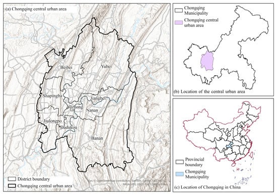
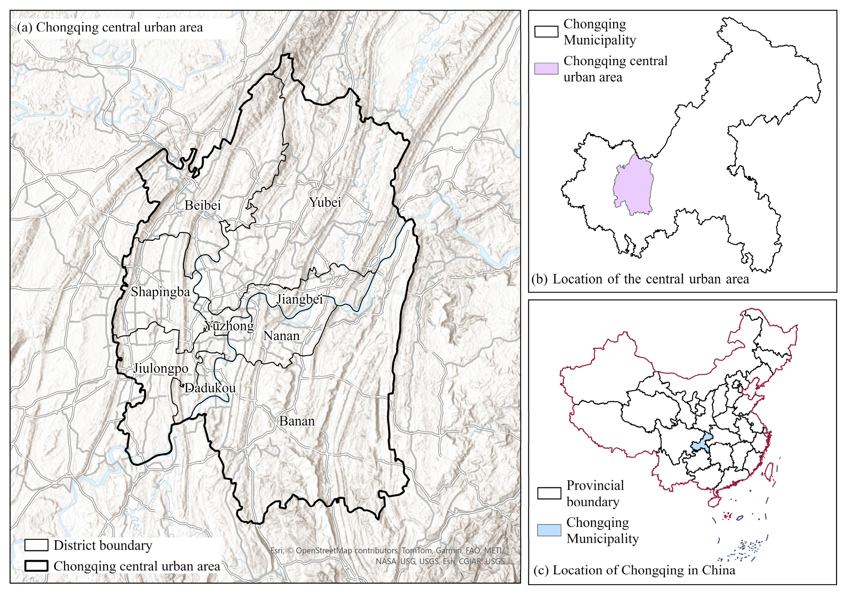
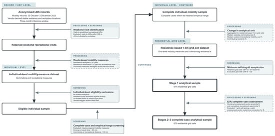
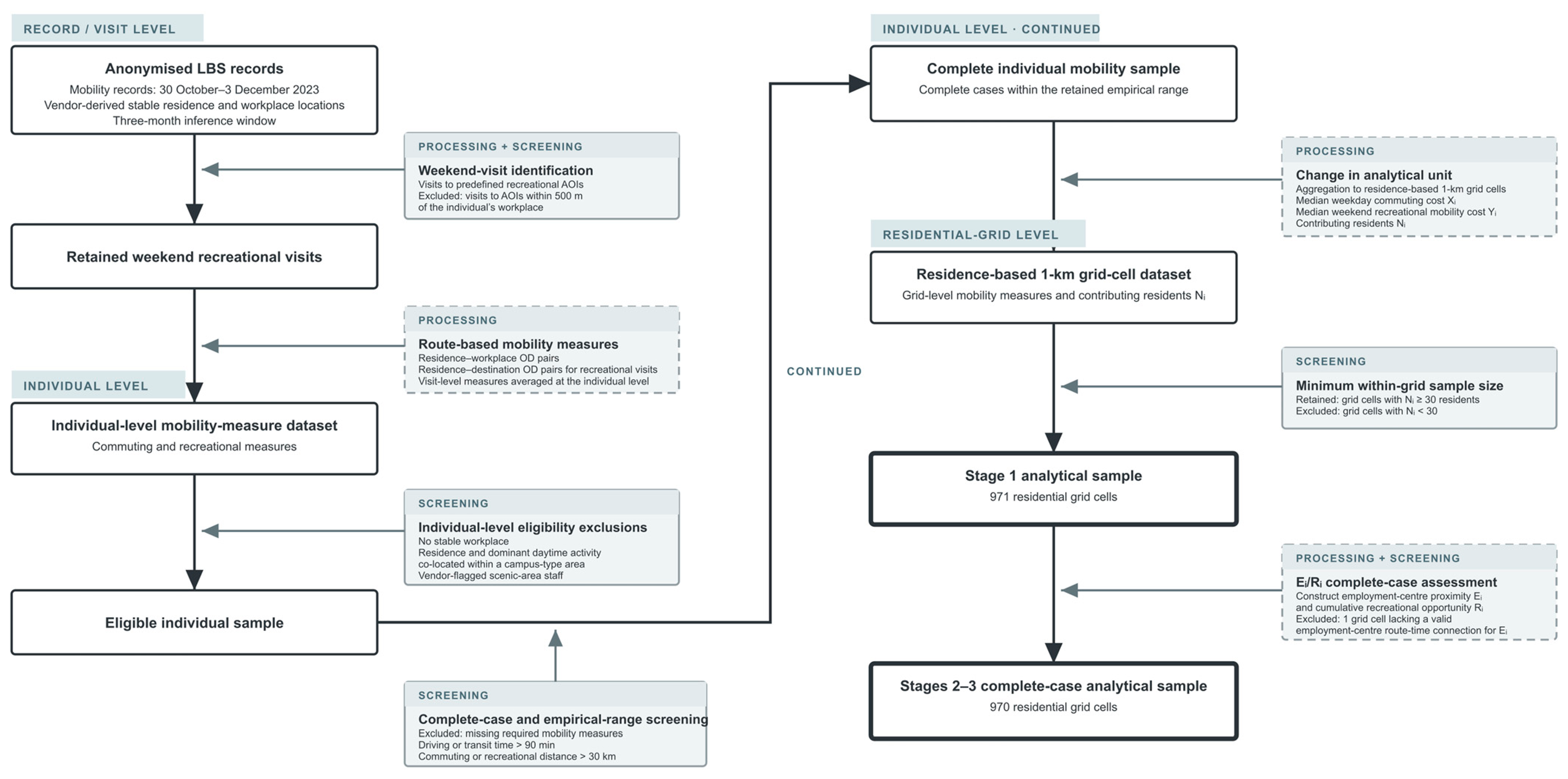
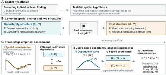
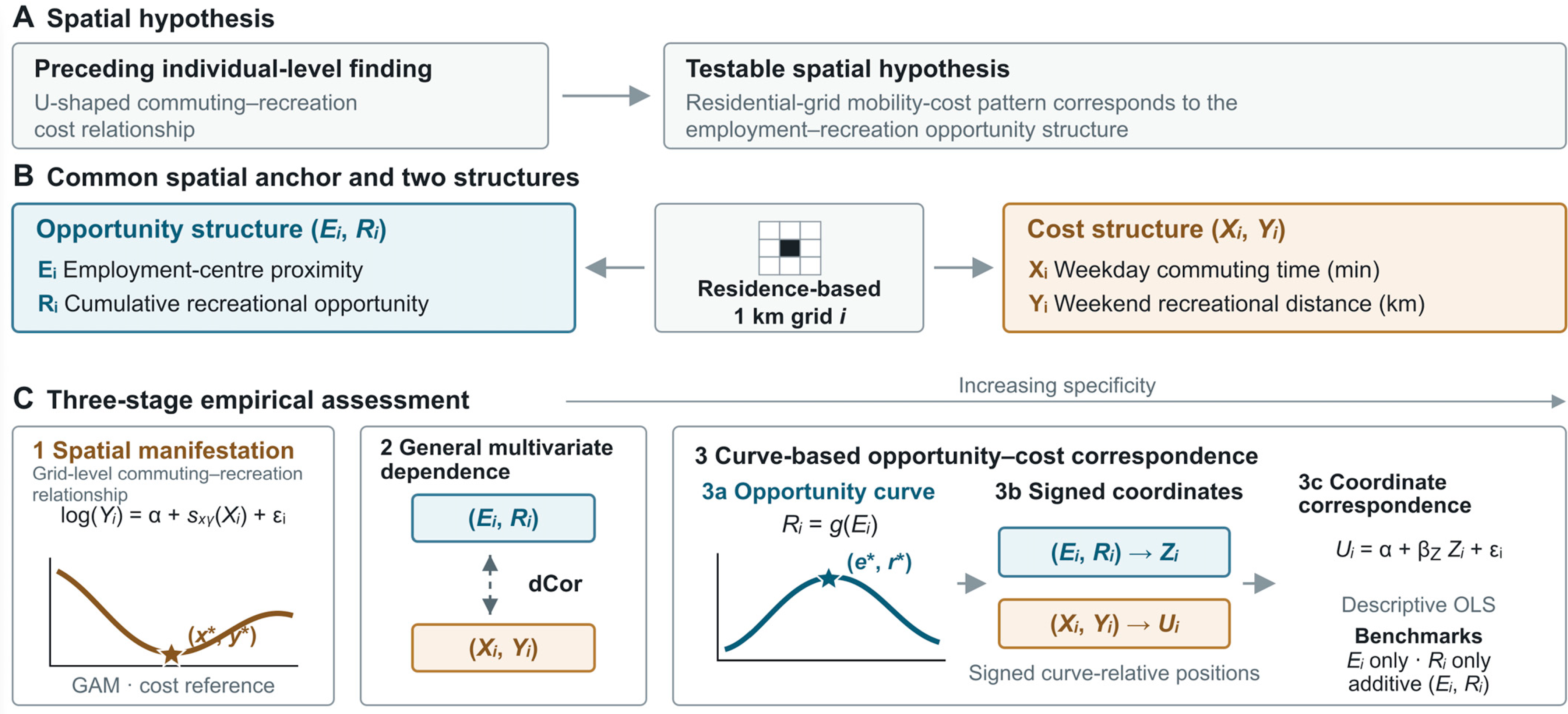
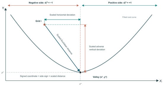
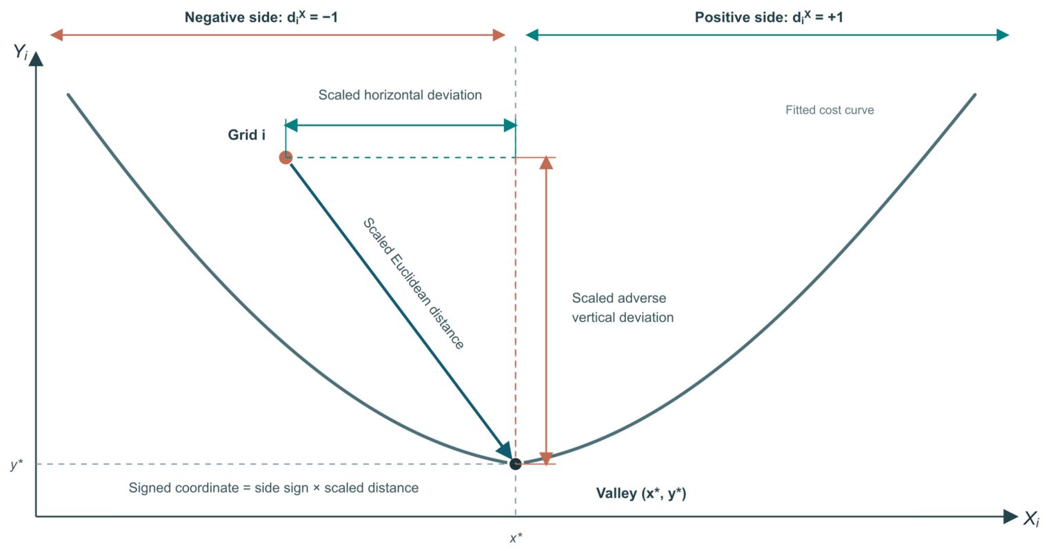
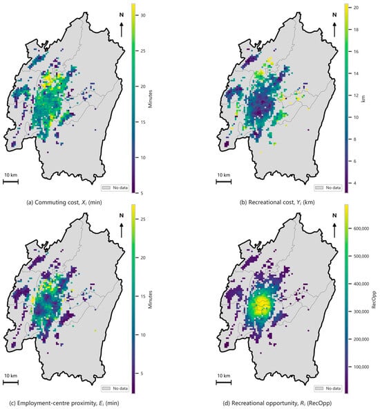
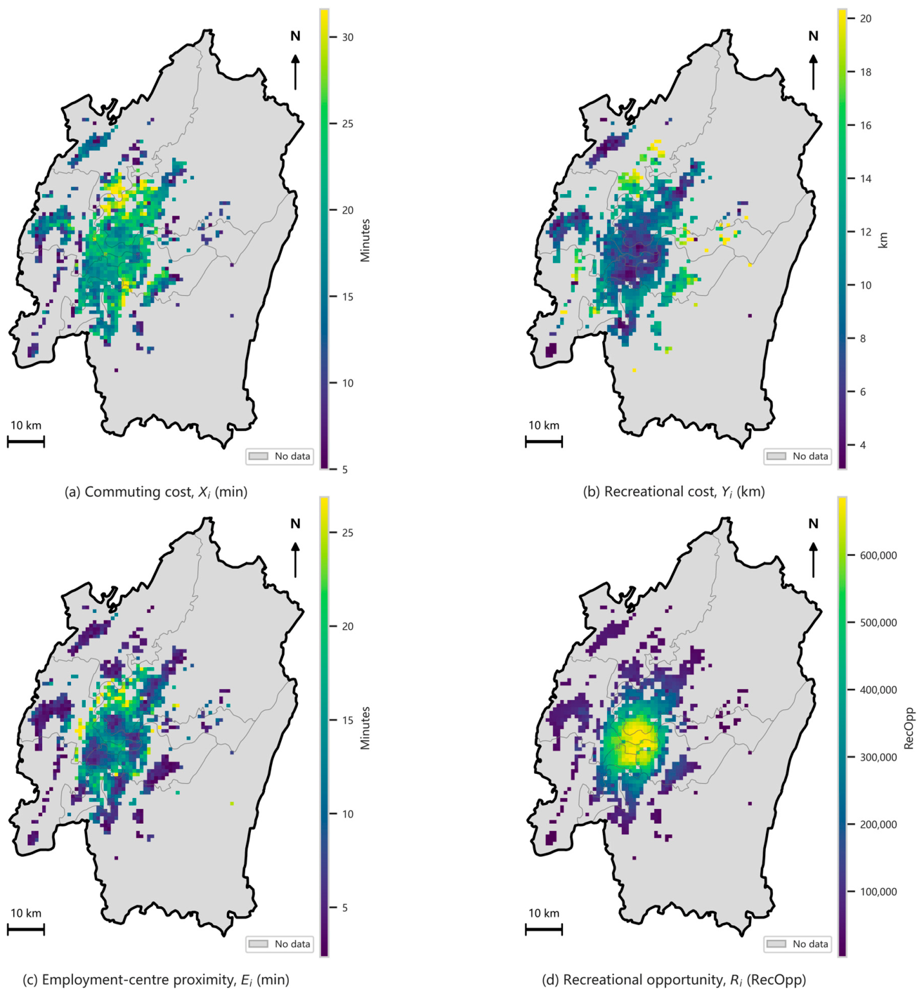
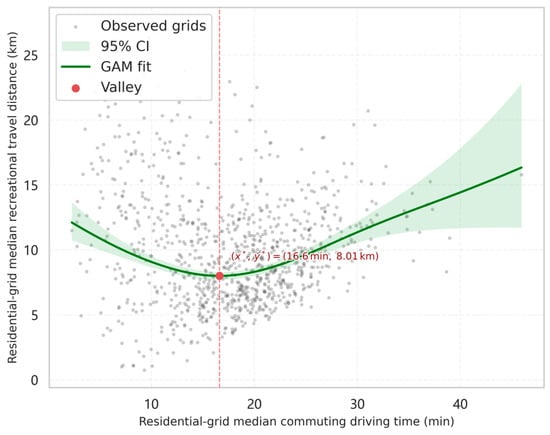
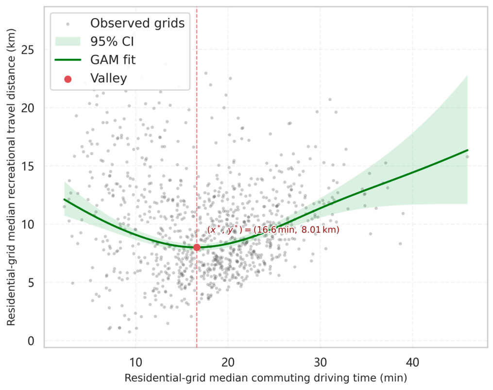
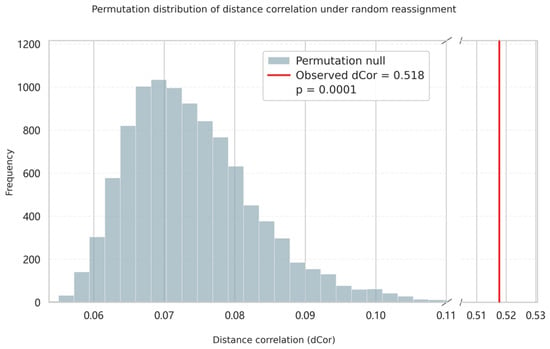
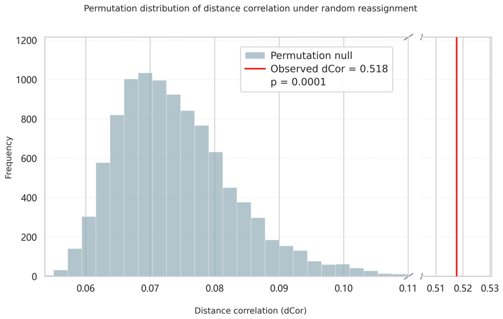
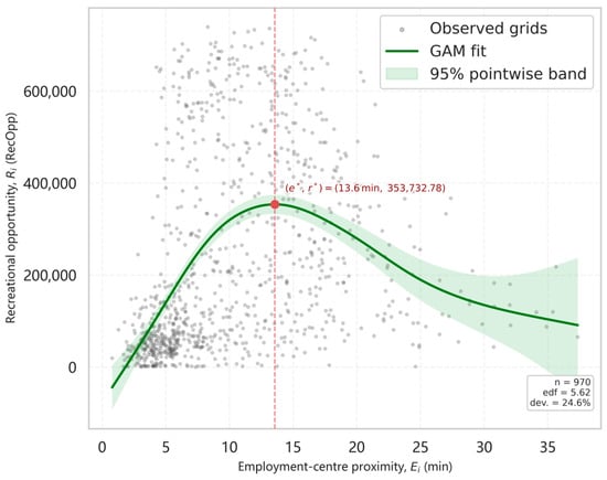
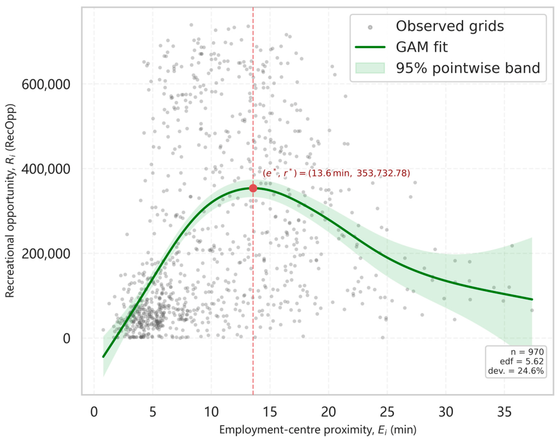
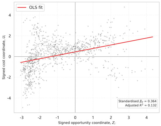
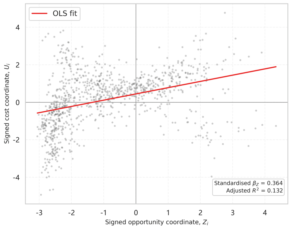

Disclaimer/Publisher’s Note: The statements, opinions and data contained in all publications are solely those of the individual author(s) and contributor(s) and not of MDPI and/or the editor(s). MDPI and/or the editor(s) disclaim responsibility for any injury to people or property resulting from any ideas, methods, instructions or products referred to in the content. |
© 2026 by the authors. Licensee MDPI, Basel, Switzerland. This article is an open access article distributed under the terms and conditions of the Creative Commons Attribution (CC BY) license.