


Abstract
Conventional applications of the CLUE-S model rely on a static driver assumption, using driver data and their associated coefficients from a base year to simulate land-use patterns for a future target year—an approach that implicitly assumes temporally invariant human–land relationships. To address this limitation, this study introduces and compares two simulation models: the Baseline-Driven Pattern (BDP), which follows the conventional protocol by employing base-year drivers to project future land use, and the Target-Driven Pattern (TDP), which instead utilizes driver data and coefficients that correspond synchronously to the target year, thereby capturing the dynamic evolution of driving mechanisms over time. In terms of implementation, the TDP involves updated driver datasets and regression coefficients, enabling a more accurate spatial allocation of land-use demand. Comparative experimental results from Xiamen in China demonstrate that the TDP achieves higher simulation accuracy than the BDP simulation, with notably greater sensitivity to dynamic factors such as transportation infrastructure and policy boundaries. For study periods 1989–2000 and 2000–2010, the accuracy of TDP simulation for all land-use types surpasses that of BDP simulation. As time progresses, the advantage of TDP simulation over BDP simulation becomes more pronounced, resulting in a significant improvement in the simulation accuracy. These findings confirm that the temporal alignment between driver data and the simulation period is a critical determinant of CLUE-S simulation accuracy. This methodological refinement holds significant implications for model-based land-use planning: it allows simulation procedures to explicitly incorporate future driver conditions articulated in planning documents. Moreover, it equips decision makers with a more realistic simulation tool for evaluating the land-use consequences of alternative planning interventions in scenario-based analyses.
1. Introduction
Land-use research serves as a critical foundation for understanding, quantifying, and managing ecosystem services, as it directly links human activities with ecological functions and service outcomes [1,2]. The complexity of land-use changes arises from the interaction of a confluence of factors, namely human, socio-economic, and natural environmental influences, which operate concurrently [3,4]. Simulation and prediction of future land-use changes are crucial aspects of LUCC research and represent significant facets of experimental ecosystem control [5,6,7].
Within this context, the CLUE (Conversion of Land Use and its Effects) model is particularly notable for its ability to integrate and assess the combined effects of human, socio-economic, and natural environmental drivers on land-use change [8,9,10]. It serves as a comparative approach for research on land use/cover change [11]. Additionally, the Dyna-CLUE model is its most advanced version with cross-scale capability in land-use simulation [12,13,14]. Model validation encompasses techniques to ensure simulation accuracy [15,16,17]. Spatial accuracy was assessed via cell-by-cell map comparison using Kappa coefficients—a widely used metric for measuring overall consistency between two maps [18,19,20,21].
Jianzhou Gong emphasized that further efforts are needed to improve the model’s predictive accuracy, given its limitations and uncertainties, especially regarding low outcome accuracy [22,23]. For better calibration and validation in modeling, cross-model comparisons have revealed the multidimensional nature of model accuracy. van Vliet’s comparative study of multiple models demonstrates the potential of temporal deep learning in improving the accuracy of annual and dense time-series land cover mapping [15]. Pontius et al. (2008) showed that quantity and allocation accuracy vary considerably across models [8]. Pickard et al. (2017) introduced configuration accuracy as an additional dimension, noting that models excelling in quantity and allocation may poorly simulate landscape configuration [24]. Jiang et al. (2015) addresses the issue that traditional logistic regression ignores spatial autocorrelation, thereby improving simulation accuracy [25].
Increasing spatial resolution is a potential approach for accuracy improvement [26,27]. However, for CLUE-S, research shows that higher resolution may actually reduce simulation accuracy due to increased complexity and noise, which can exceed the processing capacity of CLUE-S [8]. To address the current limitations in land-use simulation accuracy, regional variability of land change proves to be a key determinant [28,29]. Da Lü advocated accounting for region-specific drivers of land-use change to enable more accurate predictions tailored to different areas [28]. Guitang Liao suggested that incorporating regional drivers such as landform type, climate type, and planting systems can improve simulation accuracy in multi-region studies [29]. However, these approaches have yet to be fully implemented and validated.
Another approach to enhance accuracy is model integration. Ping Zhang coupled CLUE-S with SWAT, improving simulation reasonableness and accuracy under different scenarios for effective non-point source pollution assessment [30]. Wenkai Bao integrated CLUE-S with Markov to overcome single-model limitations, achieving high accuracy and demonstrating Dyna-CLUE’s potential for large-scale urban agglomeration areas [31].
Despite these efforts, model integration does not resolve inherent issues within CLUE-S nor identify the optimal coupling model. Moreover, incorporating region-specific drivers may compromise CLUE-S’s universal applicability, and it remains to be fully implemented and validated.
Furthermore, according to Yang et al., a substantial drawback of the model is that it does not reflect how driving factors quantitatively influence different land-use types over time. This omission may lead to inaccuracies, particularly in long-term land-use simulations. Therefore, it is imperative to integrate practical methods capable of dynamically updating the regression parameters within the simulation process [32,33].
The traditional application of the CLUE-S model operates on a foundational premise: future land distribution is simulated by projecting the target land-use demands using driver variables from a baseline period, assuming that the underlying relationships between land use and its drivers remain static over time [16]. Thus, traditional application of the CLUE-S model is essentially a sort of target-driven forecasting. While widely adopted, this conventional approach harbors a fundamental temporal inconsistency. It implicitly assumes that the spatial determinants of land use in a future period are adequately represented by the socio-economic and environmental conditions of a past period. We therefore propose the hypothesis that simulations can be improved by utilizing driver data specific to the target year itself.
To validate this hypothesis, a controlled experiment was designed [34]. One simulation used historical data of driving factors from the initial year, while the other simulation utilized updated driving factor data from the target year. The aim of both sets of experiments was to compare the simulation results and to test the accuracy improvement under different driving factors and mechanisms [32,33]. By systematically quantifying the discrepancy in simulation accuracy between these two models, this research seeks to provide a robust assessment of the sensitivity of the CLUE-S framework to temporal mismatches. The findings of this research are intended to offer an essential methodological refinement that if the results demonstrate that the new simulation design indeed enhances accuracy, it would provide novel insights and innovative extensions for the CLUE-S application, as well as a more realistic framework for projecting future land-use dynamics in an era of rapid environmental and socio-economic change.
2. Materials and Methods
2.1. Research Hypothesis and Framework
2.1.1. Research Hypothesis
As Yang et al. have pointed out, the original CLUE-S framework fundamentally overlooks the continuously evolving interplay between land-use types and their driving factors. Thus, in the simulation process, practical methods should be used to dynamically update the regression parameters [32,33].
It is hypothesized in this research that the simulation accuracy of the model is sensitive to the temporal alignment between input driver data and the simulation period. This means that the simulations employing drivers and coefficients that are temporally synchronized with the target year would achieve higher accuracy in land-use spatial allocation compared to conventional static-driver simulations.
To test this hypothesis, a comparative experiment is designed: the BDP model follows the conventional approach using base-year drivers, while the TDP model utilizes updated driver data from the target year. By systematically quantifying the accuracy discrepancy between the two models, this research aims to assess the sensitivity of the CLUE-S framework to the temporal alignment between driver data and simulation period. The innovation of this study lies in treating “temporal synchrony of driving mechanisms” as an independent methodological variable within CLUE-S simulations, offering a modeling framework that more faithfully represents the dynamic nature of human–land interactions.
2.1.2. Research Framework
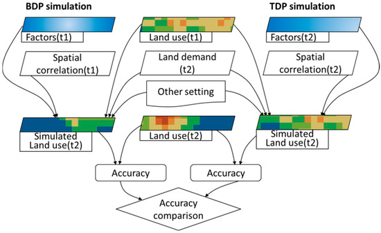
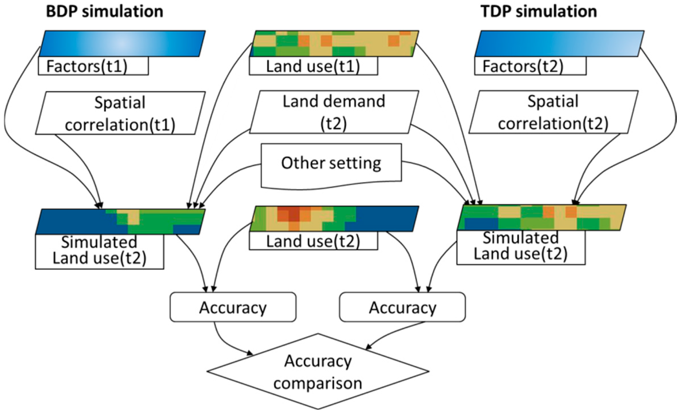
The simulation compares two methodological patterns: the Baseline-Driven Pattern (BDP), using historical driver data from the initial year, and the Target-Driven Pattern (TDP), using updated data from the target year. Each pattern independently simulates the land-use spatial distribution for the target year. The experimental configuration for the two simulation patterns is illustrated in Figure 1.
Figure 1.
Flowchart of the controlled experimental setup comparing the Baseline-Driven Pattern (BDP) and Target-Driven Pattern (TDP) in the CLUE-S simulation.
As shown in Figure 1, the BDP simulation relies on driving factors and coefficients derived from time 1 (initial year), while the TDP simulation uses those from time 2 (target year). For specific files and parameter settings during the simulation process of the two models, please refer to the next section. After the simulation, the accuracy of the two simulation methods was calculated and compared to verify the validity of the hypothesis.
2.2. Simulation Methods
2.2.1. Baseline-Driven Pattern (BDP)
The current method for the CLUE-S model to simulate land-use changes is characterized by the following principles and rules:
The raster maps of driving factors are generated from data at the initial year, with the correlation coefficient being calculated between the land use and its drivers in the baseline year [35]. Meanwhile, it uses future land demand (the “demand.in1” file, based on the setting in the target year) to calculate the land-use spatial distribution in the target year. It takes data from the initial year as its inputs, such as the existing land-use distribution, relevant driving factors, and their established correlation coefficients. This calculation method bears resemblance to the concept of Laplace’s demon and reductionism, but it fails to reflect the influence of decision makers on future planning [36,37,38]. Since the decision makers’ planning pertains to the future, this influence cannot be reflected in the established historical functional relationships of the present. Moreover, using future land demand while simultaneously relying on baseline driving factors (in initial year) would create a clear inconsistency and anachronistic situation, like using yesterday’s map to navigate tomorrow’s terrain. To avoid confusion over abbreviated names, the traditional simulation pattern is named Baseline-Driven Pattern (BDP).
2.2.2. Target-Driven Pattern (TDP)
Considering that traditional application of the CLUE-S model is essentially a sort of target-driven forecasting that inconsistently uses drivers and a correlation coefficient in the baseline year, this study adopts complete target-driven forecasting with updated driving factors and mechanisms. In this approach, the impact of decision makers’ objectives on future urban planning, such as road networks, would be considered the impact factors. This optimized method for land-use simulation requires the consideration of various conditions under future objectives, which may differ significantly from the current situation, fully considering the fact that driving factors and mechanisms are changing over time [32,33]. While traditional simulation methods exhibit strong empirically validated regularities, they prove inadequate and unscientific in simulating or predicting outcomes for future multi-objective decision making regarding the future. In other words, they fail to provide reasonable forecasts for land-use structures under future objective scenarios and neglect the change in driving factors and mechanisms [32,33].
The land-use distribution in the future is influenced by various determinants, with different impact factors. Therefore, when simulating the optimization of land-use distribution, it is advisable to construct an interactive optimization model. Such a model enables both planners and decision makers to observe the differences between different target scenarios and traditional simulation methods [37]. Moreover, it allows for the adjustment of model parameters based on decision makers’ preferences for different objectives [36,37,38].
In brief, since traditional application of CLUE-S is essentially target-driven forecasting, we believe that, where possible, the driving factors of the target year should be used. Specifically, the approach that combines the driving factors of the target year with future land demand (for the target year as well) should be adopted in place of the approach that combines future land demand with the driving factors of the baseline time nodes.
It should be noted that, if for historical data and verifying the applicability of the model and the effectiveness of the driving factors (such as in this study), the simulation is using actual observed driver data from the target year to simulate that same target year’s land use (a validation test before simulation for the future), referring to Table 1; if for future land distribution, the simulation is using projected/exogenous target-year driver data [39,40]. Thus, the data should be derived from planning documents.
Table 1.
The setting of simulation files for two patterns over three periods.
Further, for most situations in this interactive optimization simulation approach, socio-economic factors and anthropogenic factors are more prone to updating to the target year, whereas natural factors (which are less subject to human intervention) are less so. In this research, factors that will remain unchanged in the future include distances to the coastline, district centers, town centers, elevation, slope, etc., and factors that will change based on target expectations and decisions include the distribution of road networks.
2.2.3. Simulation Model
The CLUE-S model is a spatially explicit, grid-based simulation framework for projecting and analyzing land-use changes [35,41]. Key features often include a multi-criteria evaluation for suitability assessment, scenario-based planning capabilities, and tight coupling with geographic information system (GIS) for data processing and visualization [42,43,44]. It integrates socio-economic drivers, spatial constraints, and neighborhood interactions through a cellular automaton (CA) core, which determines transition probabilities for each land parcel based on a suite of explanatory variables [45]. The version of the CLUE-S employed in this research is Dyna-CLUE, available on the official repository and published by Peter Verburg, “https://www.environmentalgeography.nl/site/data-models/data/clue-model/ (5 March 2025)” [12].
The CLUE-S model operates on two core assumptions. First, land-use changes in a given region are primarily driven by land-use demand. Second, the spatial distribution of land use in that region is always in a state of equilibrium with the natural environment, land requirements, and socio-economic conditions [35]. The CLUE-S model comprises two core components that manage land-use demand (via the demand.in1 file) and the spatial distribution attributes of driving factors (via the sc1gr*.fil file). Under conditions such as land-use restriction areas (via the region_park1.fil file), land-use conversion rules (via files of alloc1.reg, allow.txt, main1), baseline land-use status (via the cov_all.0 file), and land-use spatial distribution probability, the module iteratively allocates land demands spatially based on the magnitude of the overall probability [22,23].
The spatial simulation-related parameters are set up as the following (Table 1):
- Selection of driving factors. Based on the availability of data, comprehensiveness of driving factors, and their correlation with land-use change, factors of the elevation data along with the slope are selected as drivers from the natural environment. For the socio-economic aspect, distance factors like road networks (DR), centers of districts and towns (DDC and DTC), and coastlines (DC) are chosen [46].
- Restricted areas. The regional constraint file covers the entire scope of Xiamen City. Control over the transitions among all the land-use categories is achieved through the establishment of transition matrices. Values within these matrices are limited to 0 or 1, where 0 signifies no transition is allowed and 1 indicates permissible transition.
- Land demand and allow matrices. The analysis uses the spatial distribution data for all land-use categories in initial year as the base data and takes the land amount in target years of 2000 and 2010 as its land demand data. Based on whether land transfers actually occurred or not during the historical period for simulation, the allow matrices were set.
- Conversion rules for land-use type. Defined on a continuous scale from 0 to 1, the conversion elasticity coefficient represents the resistance to land-use change, where values approaching 0 correspond to high transferability, and those nearing 1 indicate stability.
Like the allow matrices, the elasticity coefficients were determined based on historical land-use change data and were therefore independent of the simulation method. Consequently, the coefficients remained consistent across both simulation scenarios across all stages and were set as follows: watersheds 0.2, built-up land 0.9, farmland 0.2, forest land 0.9, and grassland 0.2.
2.2.4. Accuracy Evaluation of Simulation Experiments
The accuracy evaluation of the CLUE-S model includes two parts:
(1) Factor validation. Driving factors from the logistic regression were evaluated for their explanatory power against a standard ROC (receiver operating characteristic) benchmark of 0.7. Given that ROC values fall between 0.5 and 1.0, exceeding this threshold validates the selected factors as having good explanatory capability for the observed land-use types [8]. Thus, building on these validated driving factors, the CLUE-S model offers a robust tool for simulating the spatial allocation of various land-use types.
The simulation is divided into three stages: using data from 1989 for spatial simulation in 2000, using data from 2000 for spatial simulation in 2010, and using data from 1989 for spatial simulation in 2010.
For all time periods studied, the six driving factors demonstrated strong explanatory power, with ROC values consistently above 0.7. Consequently, the derived regression equations were deemed reliable for characterizing the driver–land-use dynamics and served as direct inputs to parameterize the CLUE-S model.
(2) To assess the simulation accuracy of the CLUE-S model, the Kappa coefficient is used as the quantitative evaluation metric [47], namely the consistency between the simulation results (predicted change) from the CLUE-S model and the actual distribution situation (observed changes in the land use). This comparison is obtained by juxtaposing land-use status data and simulation data at the same time point [48,49,50]. Such comparison can be achieved by spatial overlay analysis in ArcGIS 10.0 software. Generally, Kappa values were categorized into agreements as slight with low simulation accuracy (<0.4), moderate (0.4–0.7), and high (0.7–1) [18,19,20,21].
It is important to note that no universally accepted threshold exists for interpreting Kappa values as “acceptable” or “unacceptable”; rather, the coefficient is most appropriately used for relative comparisons among different simulation approaches or temporal stages, thereby providing insight into model performance consistency rather than an absolute measure of predictive accuracy [8].
The specific calculation for Kappa coefficient is shown in the following formula:
where Po refers to the actual proportion of grids simulated correctly. Pc defines the correct proportion expected from a random classification, equivalent to the reciprocal of the total simulated land-use types. Pp corresponds to the proportion correct under perfect classification, which is always 1.
2.2.5. Experimental Instance and Study Area
This investigation employs a coastal Chinese city, Xiamen, as a case study to implement comparative experiments. As one of the earliest economic special zones to undergo reform and opening-up policies in China, Xiamen is a city with highly developed industrialization and urbanization. Since the 21st century, with the intense development of land resources, Xiamen has undergone drastic changes in land-use distribution, with urbanization rates exceeding 90%.
The digital elevation model (DEM) and land-use data in this study were obtained from the data center at the Institution of Urban Environment, Chinese Academy of Sciences. Specifically, the two datasets were derived from SRTM data and Landsat TM satellite imagery. Additionally, the land use with the resolution of 30 × 30 m is categorized into five types: farmland, forest land, watersheds, grassland, and built-up land. Road network data are actual infrastructure data for each year (1989, 2000, and 2010) and are derived from maps by the Xiamen Planning Bureau.
Factors such as slope information were extracted from the DEM data using ArcGIS software, while distance factor data were computed within the same software employing the metric of Euclidean distance. The calculation procedures are as follows:
Distance to Roads and Railways: Based on the vector data mentioned above, the “Spatial Analyst Tools” in ArcGIS software was utilized to calculate the straight-line distance from each raster cell to the nearest road networks (including expressways, national highways, and provincial roads) and railway lines.
Distance to Coastline: Similarly, the Euclidean distance from each raster cell to the nearest coastline (including both the mainland coastline and major island coastlines) was calculated.
The distances to the city center and town center were calculated using the same method.
3. Results
3.1. Simulation Results Using BDP Methods and Comparison with Actual Data
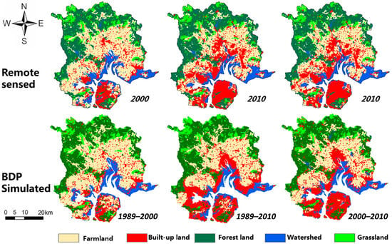
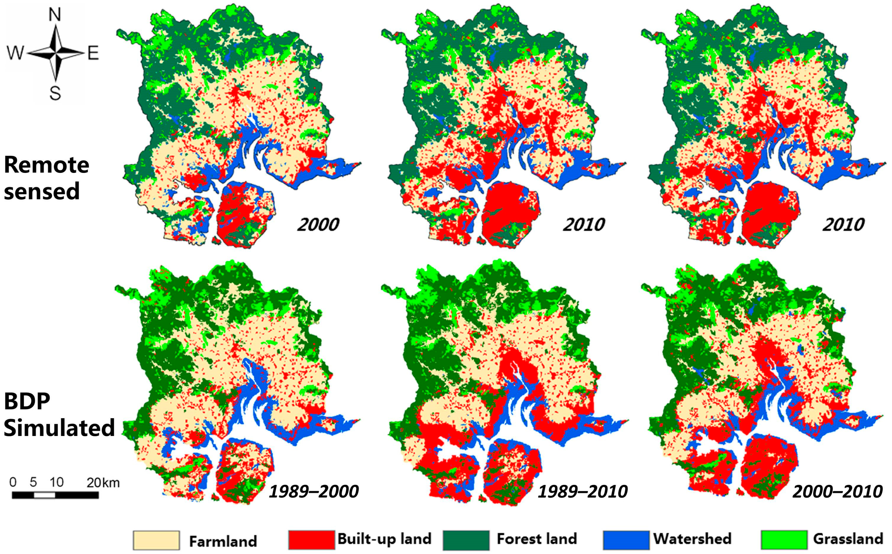
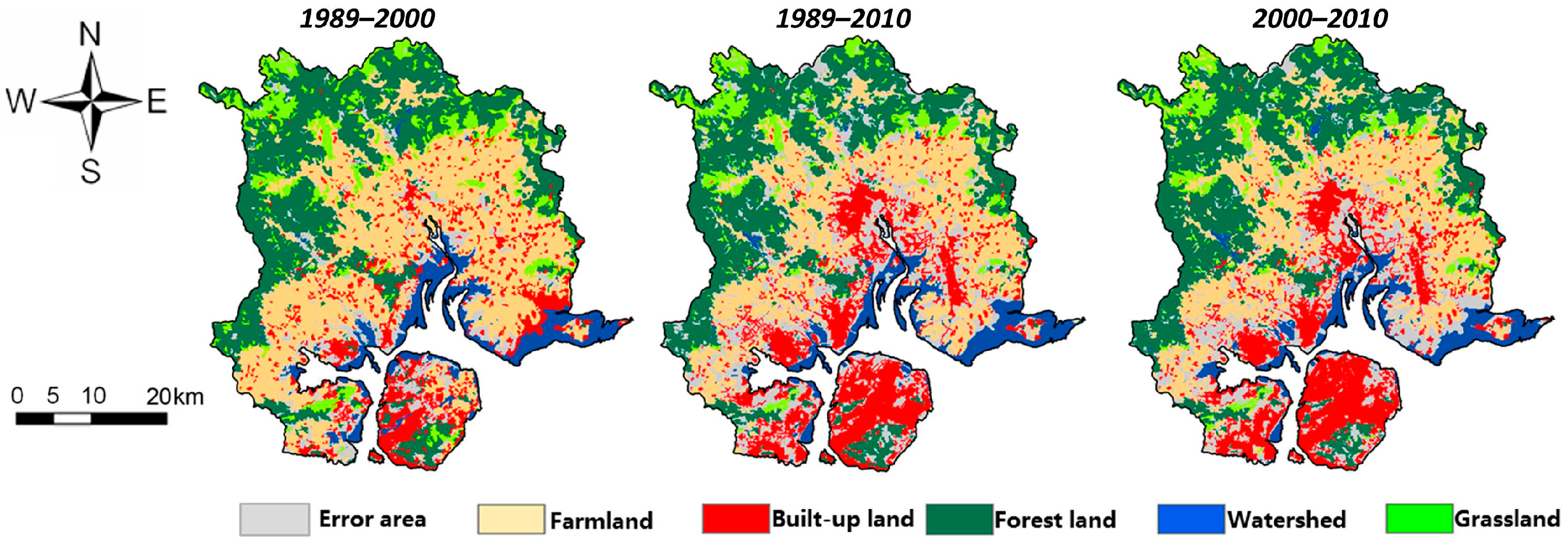
A comparative view of actual and simulated land-use allocations across the three study periods (1989–2000, 2000–2010, and 1989–2010) is presented in the following figure (Figure 2). As shown in Figure 2, the simulated maps largely resemble the actual maps. However, there are some differences near the coastline, particularly concerning built-up areas and watersheds [51]. To further describe these differences quantitatively, raster calculations and analyses were performed on the actual and simulated maps using ArcGIS.
Figure 2.
Spatial distribution of actual versus BDP-simulated land use in Xiamen City.
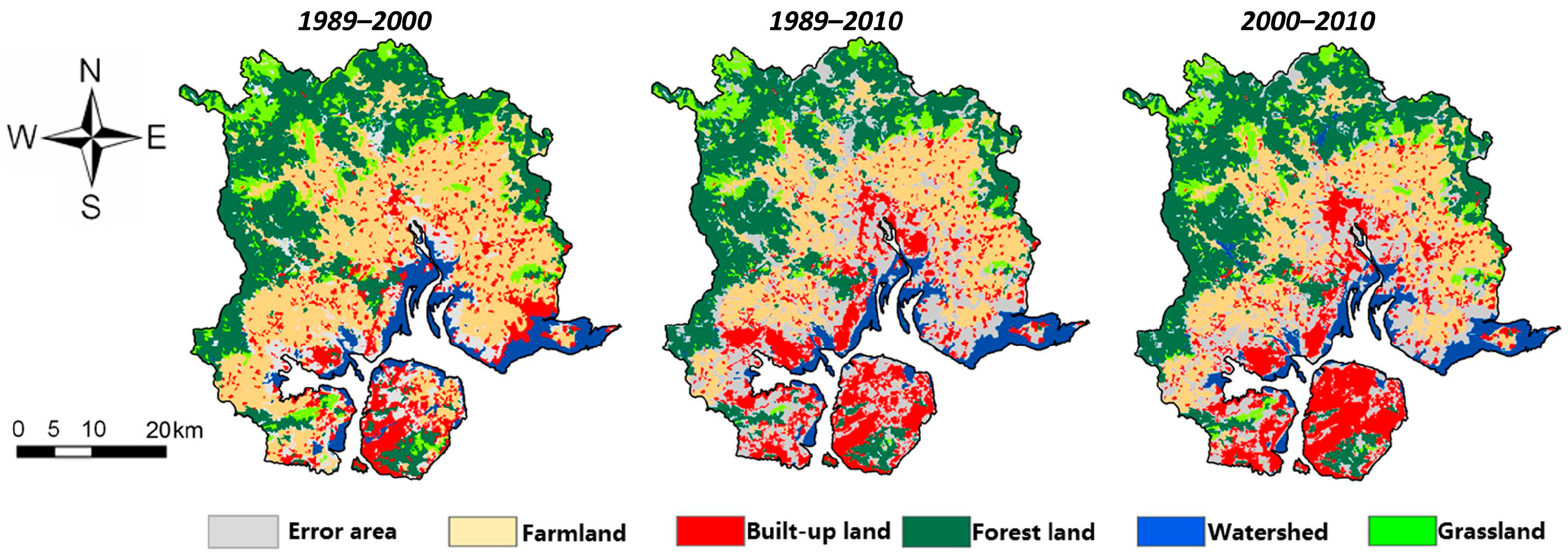
Using the Raster Calculator tool in ArcGIS, the land-use maps at the end of two time nodes (2000 and 2010) were compared with the simulated land-use maps by performing raster subtraction. The number of zero-value cells represents the correctly simulated grids. The results of this calculation are shown in the figure below (Figure 3).
Figure 3.
Spatial distribution of BDP simulation accuracy for 3 periods.
The gray areas on the map, which indicate simulation errors, reveal that the spatial distribution of errors across the three periods occurs mainly around the coastline and the original built-up areas. These calculation results corroborate previous observations regarding the spatial distribution of simulation errors.
Based on the number of correctly simulated grids, further accuracy calculations and Kappa tests were conducted. If we take the period from 1989 to 2000 as an example, the number of zero-value grids accounted for 90.1% of the total grid count (accuracy rate). According to the Kappa formula, this gives Po = 0.901. With five land-use categories, the random correct rate for a single land-use type is 1/5. Thus, Pc = 0.2. Consequently, the Kappa value is calculated as Kappa = 0.876, which is greater than 0.75, indicating a relatively ideal accuracy. Table 2 shows the accuracy results for the three periods.
Table 2.
Simulation accuracy for BDP scenario over three periods.
As shown in the table, the overall accuracy results show that the simulation accuracies for the three periods are ranked as follows: 1989–2000 > 2000–2010 > 1989–2010. This ranking indicates that, as the time span increases, regional land-use changes become more pronounced, leading to a decrease in accuracy. The period 1989–2010, in particular, fails to pass the Kappa test with an accuracy of only 67%.
As observed in the performance of the five land-use categories across different periods, the accuracy rankings are as follows:
From 1989 to 2000: grassland > forest land > farmland > built-up land > watersheds, with watersheds having the lowest accuracy among the five categories (74.8%).
From 2000 to 2010: forest land > grassland > farmland > watersheds > built-up land, with watersheds ranking second to last.
From 1989 to 2010: forest land > grassland > watersheds > farmland > built-up land, with watersheds ranking third (72.1%).
In all three periods, the accuracy for watersheds is consistently below 75%, indicating relatively low accuracy. Similarly, the accuracy for built-up land and farmland is also comparatively low. These statistical results align with the earlier observational findings.
3.2. Simulation Results Using TDP Methods and Comparison with Actual Data
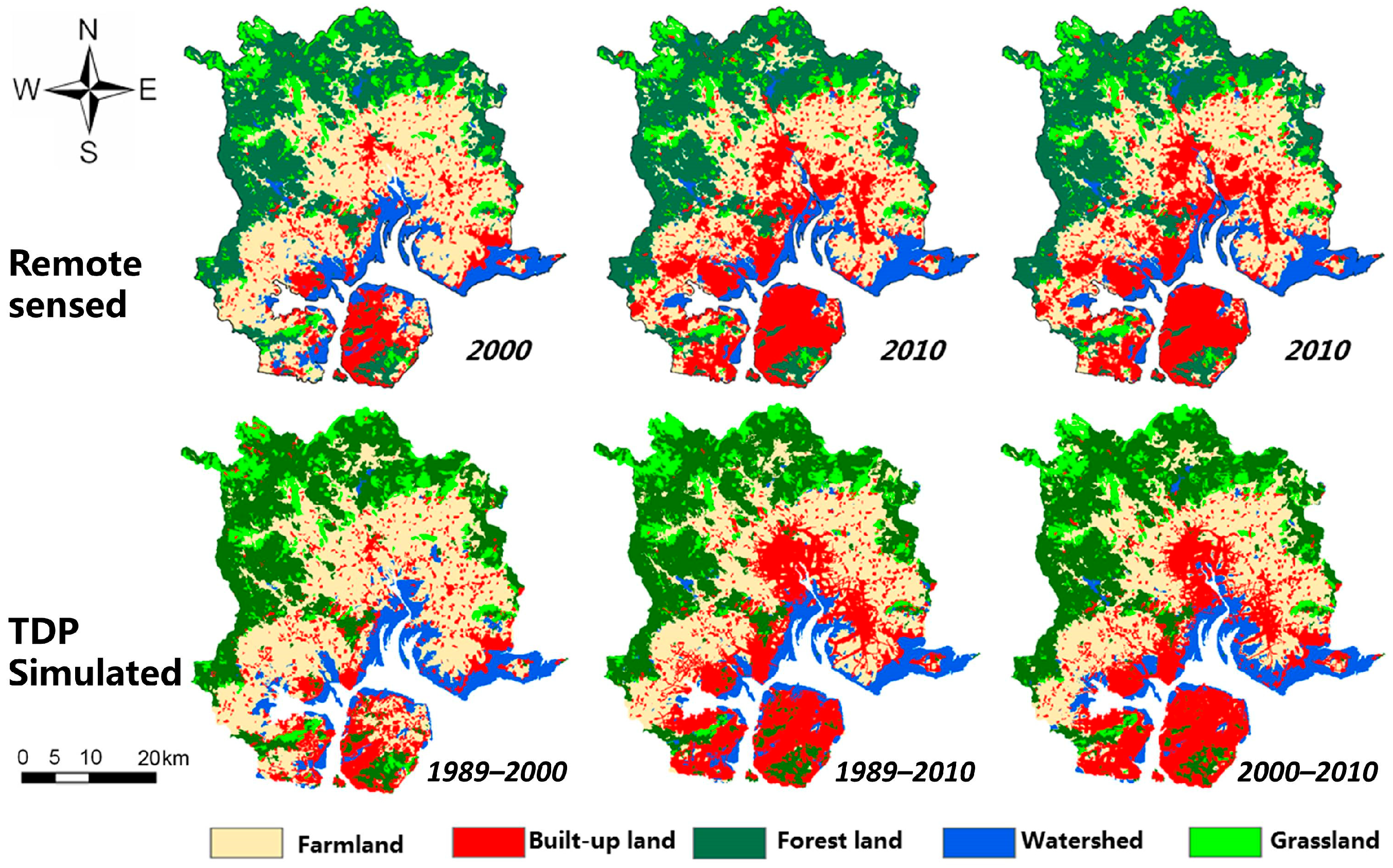
Similarly, a comparative view of actual and simulated land-use allocations across the three study periods is presented in Figure 4. Compared to the BDP method, the simulation errors in the TDP simulation have been greatly reduced in the vicinity of the coastline. To further describe the improvement achieved by the TDP simulation effect with data, raster calculations and analysis were performed in ArcGIS.
Figure 4.
Spatial distribution of actual versus TDP-simulated land use in Xiamen City.
Similarly, raster subtraction was conducted using the Raster Calculator in ArcGIS between observed land use from remotely sensed maps and the TDP-simulated maps. The number of zero-value grids represents the correctly simulated grids. This calculation result is displayed on the map as shown in Figure 5.
Figure 5.
Spatial distribution of TDP simulation accuracy in three periods.
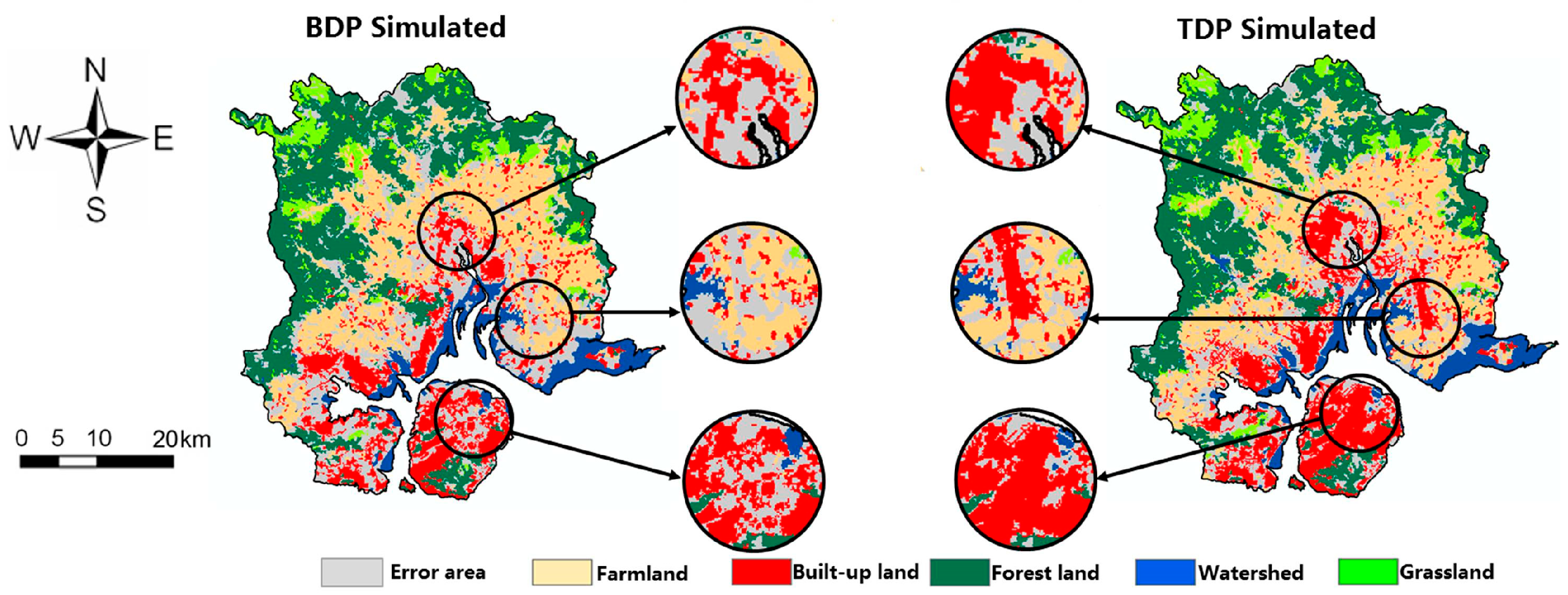
In Figure 5, the gray areas indicate the spatial distribution of simulation errors. It is evident that, although the TDP method still shows errors mainly around the coastline and original built-up areas, there has been significant improvement in the periods of 1989–2010 and 2000–2010. Specifically, the extent of error distribution in the coastal zone has greatly decreased with the TDP simulation method. For instance, when one compares the simulation results from 2000–2010, a magnified view of a selected area reveals that the error distribution range is noticeably reduced in the results from the TDP method (Figure 6).
Figure 6.
Comparison of differences in results between BDP and TDP simulation during period of 2000–2010.
To further quantify such optimization and improvement, the results from the ArcGIS raster calculations were compiled into the following accuracy statistics table. As shown in Table 3, its Kappa coefficient in the period 1989–2010 has significantly improved to 73%, much higher than the 67% obtained with the BDP method. This improvement indicates that as the time span lengthens and land-use changes become more pronounced, the new method demonstrates a distinct advantage.
Table 3.
Simulation accuracy for TDP scenario over three periods.
Although the TDP method significantly outperforms the BDP method in the periods 2000–2010 and 1989–2010, the overall simulation accuracy across the three periods remains ordered as 1989–2000 > 2000–2010 > 1989–2010 (Table 3). This ordering indicates that the trend of decreasing accuracy over longer time spans persists. The accuracy rankings for specific land-use categories within each period also remain unchanged and will not be reiterated here.
4. Discussion
In this study, we conducted experimental simulations and data validation focused on land-use change to show that simulation with updated driving factors and mechanisms, rather than simulation with just current conditions, will more accurately simulate land-use change. Two experimental scenarios are set up for comparison: one based on current conditions and the other driven by specific objectives with updated drivers. In this study, simulations of land-use distribution changes in Xiamen were conducted for multiple time periods with two simulation methods, utilizing results from logistic regression and the CLUE-S model. The experimental outcomes are then compared with the remote sensing maps of the land use to calculate the overall simulation accuracy and the accuracy for five specific land-use types [52]. The effectiveness of the simulations was validated against the established standard of the Kappa coefficient [48,49,50]. Finally, the results of the two driving methods are compared. The comparison verifies the research hypothesis, revealing the following key characteristics.
4.1. Overall: The TDP Outperforms BDP at All Stages
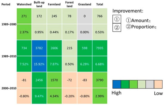
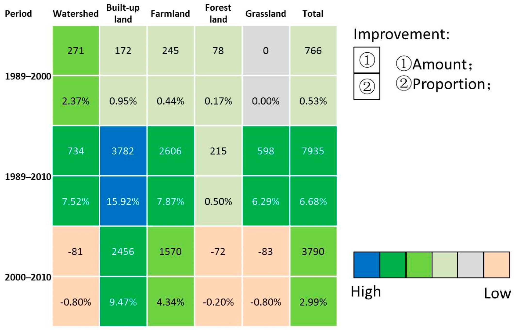
The accuracy comparison results for the two simulation scenarios—BDP and TDP—are presented in Figure 7. Both scenarios show that when calibrated with target-year driver data, CLUE-S more accurately reproduces target-year land-use patterns than when calibrated with baseline data. However, there is a notable difference in both simulation accuracy and Kappa coefficients between the two scenarios. Such results proved a conclusion that spatial distribution of the transitions would affect the simulation accuracy [34].
Figure 7.
Improvement in simulation accuracy for TDP scenario compared with the BDP scenario.
As shown in Figure 7, for the three time periods, the overall accuracy indicates that from 1989 to 2000 the accuracy of the TDP scenario is only 0.5% higher than that of the BDP scenario, suggesting a minimal difference between the two. From 2000 to 2010, the accuracy difference increases to 3.0%, with a BDP Kappa coefficient of 0.734, whereas the TDP Kappa coefficient was 0.763. For the period from 1989 to 2010, the accuracy difference between the two driving models reaches 6.68%. These results suggest that the TDP scenario provides a more reasonable prediction of future land-use spatial patterns, achieving better simulation results. The longer the time period, the greater the difference, which may be related to the magnitude of land-use changes. Further, this difference indicates that input data do indeed affect accuracy [53,54,55].
For the five specific land-use types, except for the period from 2000 to 2010 where the TDP simulations for watersheds, forests, and grasslands are slightly less accurate than the BDP simulations, the difference is minimal (<1%). However, the accuracy for built-up areas and farmlands is significantly higher in the TDP model (>4%).
To evaluate whether the difference in classification accuracy between TDP and BDP was statistically significant, we used each land-use type–time period combination as an analytical unit (N = 15). The Wilcoxon signed-rank test was applied to compare the accuracy differences between the two methods, with the significance level set at α = 0.05.
Overall, TDP achieved higher classification accuracy (mean = 81.64%, median = 79.90%) than BDP (mean = 79.99%, median = 76.50%). The Wilcoxon signed-rank test revealed a statistically significant difference between the two methods (V = 84, p = 0.014). Among the 15 land cover types–time period combinations, TDP outperformed BDP in 11 combinations and showed slightly lower accuracy in the remaining 4.
4.2. Longer Time and Greater Land Change, Lower Accuracy and Greater Gap
The accuracy table for the three periods indicates that, regardless of the driving method, the overall simulation accuracy for the three periods follows the order 1989–2000 > 2000–2010 > 1989–2010. This ordering confirms the trend that overall accuracy decreases as the time span increases. Concurrently, the total land change amount for the three periods follows the order 1989–2000 (100%) < 2000–2010 (374%) < 1989–2010 (584.8%). This inverse relationship between land change amount and accuracy suggests that as the time span lengthens and the land change amount increases, the accuracy decreases, and the difference between the two simulation methods becomes more pronounced. Therefore, for longer periods with greater land change (the land amount difference between the target and the baseline year), the TDP method proves to be more reasonable and effective.
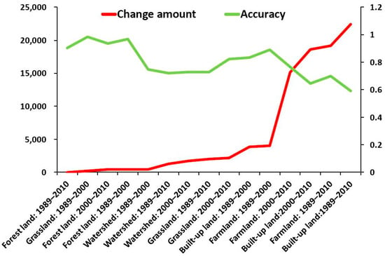
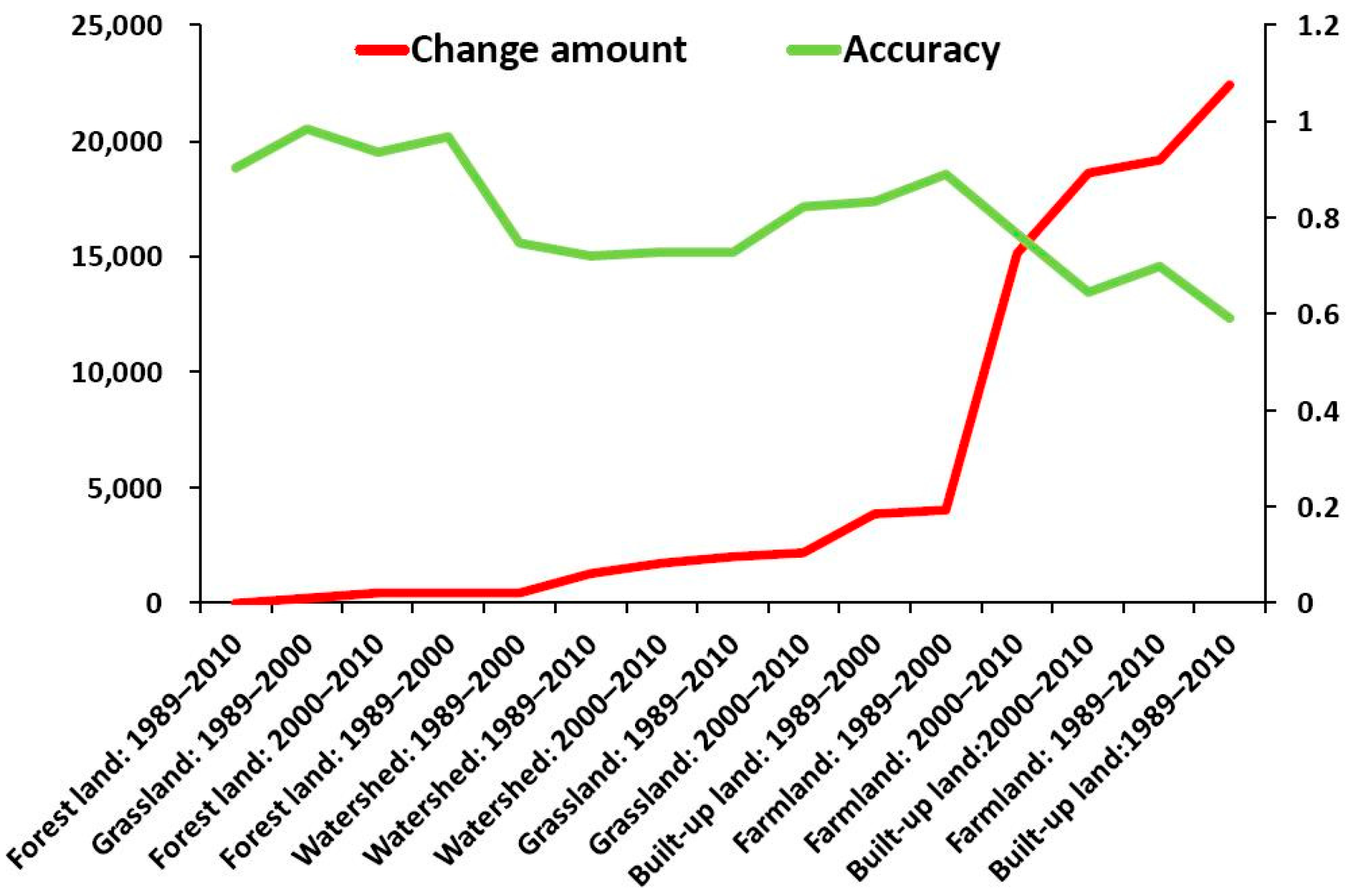
Further statistical description of the change amount and simulation accuracy of five land types over three periods is presented in Figure 8.
Figure 8.
Land-use change amount and simulation accuracy of 5 land types over three periods.
Figure 8 illustrates a near-negative correlation between the extent of land change and simulation accuracy. For instance, from 1989 to 2000, grassland, which experienced the least change, had the highest accuracy in both simulation scenarios. From 2000 to 2010, forest land, with the smallest land change, exhibited the highest accuracy (above 90%) in both scenarios, whereas built-up land, with the largest change, had the lowest accuracy (below 71%). Similarly, from 1989 to 2010, forest land, again with the smallest land change, maintained the highest accuracy (above 90%), while built-up land, with the largest change, had the lowest accuracy (below 70%). This result also indicates that there are significant differences between local and overall simulation results [56].
The figure highlights a clear trend: the greater the extent of change, the lower the accuracy.
Further, we conducted a Pearson correlation analysis in SPSS 16.0 to examine the link between change magnitude and simulation accuracy across land types and time periods. The analysis found a significant negative correlation of −0.699 and a p-value of 0.04, which confirms that the correlation is significant at the 0.05 level (two-tailed).
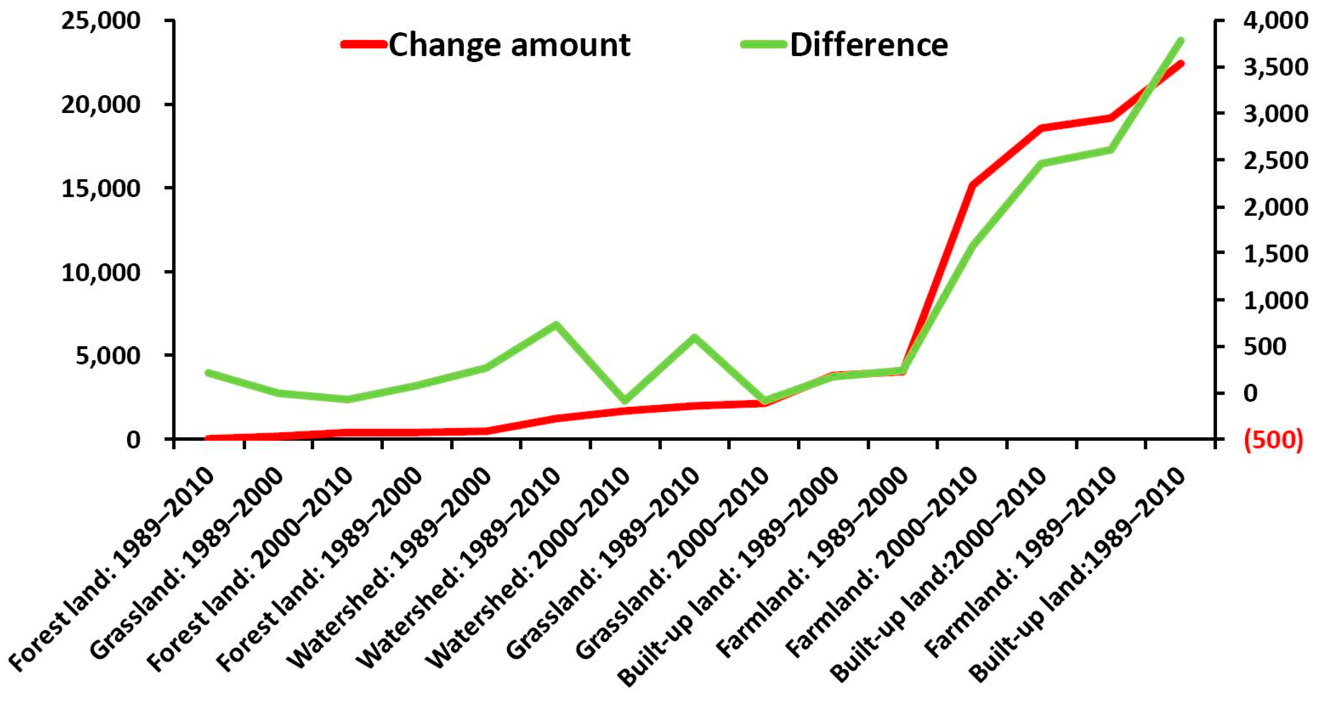
In the accuracy comparison table, the three largest differences in accuracy across all land types and time periods are as follows: built-up land in 2000–2010 (16%) > built-up land in 1989–2010 (9.5%) > farmland in 1989–2010 (7.9%). Correspondingly, the three largest changes in land area are built-up land in 2000–2010 (22,426 ha) > farmland in 2000–2010 (−19,162 ha) > built-up land in 1989–2010 (18,591 ha). The results indicate that the greater the change in land area, the more significant the difference in accuracy between the TDP simulation method and the BDP method, with the TDP method showing greater advantages. The trend between land change and simulation accuracy is illustrated in Figure 9.
Figure 9.
Land-use change amount and accuracy difference between the TDP and BDP simulation methods.
Figure 9 highlights another clear trend: the greater the extent of change, the greater the accuracy difference.
To further validate this observed difference, the relationship between land-use change amount and simulation accuracy disparity was examined via Pearson correlation analysis (N = 15) in SPSS. The results revealed a significant positive correlation between land change amount and accuracy difference (r = 0.798, t(13) = 4.774, p < 0.001, two-tailed). The 95% confidence interval for the correlation coefficient was [0.483, 0.930], indicating that greater land change is associated with larger accuracy differences.
4.3. Updated Application of CLUE-S
The early baseline-driven simulation method predicts future states based on past trends and factors. In contrast, we proposed a new approach herein that employs a teleological perspective to guide the simulation experiments. Specifically, the simulation operates by integrating target-defined parameters in future years (such as road networks) into the CLUE-S model for the projection of land-use changes [32,33].
Comparison of the results of the two sets of experiments indicates that there are consistent differences between the outcomes of the two simulation methods. Specifically, compared to those driven by the current situation (drivers in baseline year), simulations driven by objectives (drivers in target year) consistently exhibit higher accuracy, demonstrating that ecosystems can proactively respond to their objectives, yielding more optimized results.
Further, this approach not only improves the accuracy of land allocation in historical data validation but also holds significant value for future land planning and management. Additionally, this approach captures not only the dynamic evolution of human–land interactions but also reflects the intentions and influences of decision makers on future urban development [39,40].
Although decision makers’ planning intentions and goals for the future are often qualitative in nature, they are clearly articulated and knowable. Moreover, these intentions can be translated into relatively explicit driver factors (such as road networks) and correlation coefficients through planning maps. Taking transit-oriented development (TOD) as an example, this is a typical case where transportation networks shape urban land spatial patterns [57]. The transportation network planned by decision makers is knowable through planning documents, and the influence of the transportation network on land use, i.e., the correlation coefficient, is also identifiable. However, what should the corresponding land spatial distribution be? Since land spatial distribution is also influenced by factors such as topography, in this context, TDP-based land spatial simulation can provide valuable support for land spatial planning.
4.4. Limitation
Although this study systematically evaluated the performance of different simulation strategies, several limitations should be acknowledged and warrant further investigation.
First, the unavailability of driving data in predictive applications. The validation strategy employed in this study relies on comparing simulated results with actual land-use data from the same period. However, in a true predictive context—such as simulating land-use patterns for a future target year—the “actual” driving factors (e.g., socio-economic variables) for that year make it difficult to obtain precise quantitative results. Future studies should consider adopting more rigorous validation, such as extrapolation based on historical data, to more realistically assess predictive capabilities [39,40].
Second, the geographical limitations. This study focuses on a single rapidly urbanizing coastal city. While this selection allows for an investigation into simulation mechanisms within this specific context, it simultaneously constrains the generalizability of the findings. Different regions, such as inland cities, agriculturally dominated areas, or ecologically vulnerable zones, may exhibit distinct land-use change patterns and driving mechanisms [58,59,60].
Third, the risk of over-fitting. In this study, model calibration and validation were conducted using data from overlapping time periods. Although this approach is common in validation practice, it may introduce a risk of over-fitting, that is, the model may become overly tailored to the specific change patterns observed during the calibration period rather than capturing the general mechanisms of land-use change. Model performance may decline when applied to time periods not involved in calibration [15].
Fourth, sensitivity to parameter settings. The simulation results presented in this study are sensitive to the selection of driving factors and the threshold settings of validation metrics. The choice of driving factors—including their type, spatial resolution, and processing methods—directly affects the quality of model inputs and, consequently, the reliability of the simulation outcomes [39,58,59].
5. Conclusions
This study tries to test whether a purposeful simulation strategy within the CLUE-S framework enhances explanatory power and predictive accuracy for land-use change. To this end, we compared two pattern-generation ideologies: a proactive target-driven approach and a reactive baseline-driven approach, using Xiamen—a rapidly urbanizing coastal city—as a case study across three time intervals (1989–2000, 2000–2010, and 1989–2010).
Our results demonstrate that, across all three periods, the target-driven approach yielded higher overall accuracy and Kappa values than the baseline-driven approach in most cases. The performance advantage of the target-driven approach became more pronounced over longer simulation horizons. Specifically, during the 1989–2010 period, the accuracy difference between the two approaches was largest and statistically significant. Furthermore, we observed that the magnitude of this accuracy difference was positively associated with the magnitude of observed land-use change: periods characterized by greater land-use dynamics exhibited not only larger gaps in overall accuracy but also more substantial differences in class-level accuracy across individual land-use categories (p < 0.001).
These findings suggest that the target-driven approach—by incorporating updated parameter settings and a more discerning selection of driving factors—achieves superior spatial performance compared to the baseline-driven approach. However, it is important to clarify what our evidence directly supports and what remains inferential. The results demonstrate that, under the conditions tested, the target-driven approach outperforms the baseline-driven approach in terms of accuracy.
Findings also indicate, though do not establish as a general rule, that the advantage of the target-driven approach may intensify under conditions of more rapid land-use change. Whether this pattern holds across different geographical contexts, temporal scales, or land-use systems remains an open question that warrants further investigation.
From a practical standpoint, our results support the adoption of target-driven simulation strategies for urban planning applications where near-term land-use projections are needed. However, the generalizability of these findings to other regions or to longer-term forecasting should be assessed cautiously, given that our analysis was confined to a single rapidly urbanizing coastal city.
In conclusion, this study provides empirical evidence that purposeful, target-driven simulation within the CLUE-S framework yields measurable improvements in simulation accuracy under the conditions examined. Nevertheless, the specific mechanisms driving this improvement, the generalizability of the findings beyond the study context, and the performance of the approach under true predictive conditions remain important directions for future research.
Author Contributions
T.Z. was responsible for the conceptualization, methodology, and writing—original draft preparation; S.S. and G.F. were responsible for the conceptualization and writing—review and editing; G.Y. assisted with some of the visualization work; S.S. and T.Z. were responsible for the funding acquisition. All authors have read and agreed to the published version of the manuscript.
Funding
This work was supported by the Research Fund on Several Major Issues Concerning Enhancing the Security of Emerging Service Industry Systems, Zhejiang University (Grant number 2025-PP-11-09) and the Teaching Reform Project of Sichuan Normal University (Grant number JWC20250304).
Data Availability Statement
The original contributions presented in this study are included in the article. Further inquiries can be directed to the corresponding authors.
Acknowledgments
The first author extends his thanks to Lina Tang at the Chinese Academy of Sciences for research support and help with obtaining materials for the research. All authors extend thanks to the editors and anonymous reviewers for their careful work and comments, which have helped to improve this paper substantially.
Conflicts of Interest
The authors declare no conflicts of interest.
References
- Hasan, S.S.; Zhen, L.; Miah, M.G.; Ahamed, T.; Samie, A. Impact of land use change on ecosystem services: A review. Environ. Dev. 2020, 34, 100527. [Google Scholar] [CrossRef] [Scilit]
- Song, P.H.; Yang, Q.; Wu, W.Y.; Su, T.Y.; Jiang, Y.M.; Lu, J.L.; Sun, Z.Y.; Zhang, J.; Yu, R.; Wang, P.; et al. Assessing and predicting the value of ecosystem services in sanya city, Hainan island, China. Ecol. Indic. 2025, 170, 112967. [Google Scholar] [CrossRef] [Scilit]
- Liu, C.L.; Li, W.L.; Zhu, G.F.; Zhou, H.K.; Yan, H.P.; Xue, P.F. Land use/land cover changes and their driving factors in the Northeastern Tibetan Plateau based on geographical detectors and google earth engine: A case study in Gannan prefecture. Remote Sens. 2020, 12, 3139. [Google Scholar]
- Lin, A.Q.; Wu, H.; Liang, G.H.; Cardenas-Tristan, A.; Wu, X.; Zhao, C.; Li, D. A big data-driven dynamic estimation model of relief supplies demand in urban flood disaster. Int. J. Disaster Risk Reduct. 2020, 49, 101682. [Google Scholar] [CrossRef] [Scilit]
- Arndt, J.; Lunga, D. Large-scale classification of urban structural units from remote sensing imagery. IEEE J. Sel. Top. Appl. Earth Observ. Remote Sens. 2021, 14, 2634–2648. [Google Scholar]
- Talukdar, S.; Singha, P.; Mahato, S.; Pal, S.; Liou, Y.A.; Rahman, A. Land-use land-cover classification by machine learning classifiers for satellite observations—A review. Remote Sens. 2020, 12, 1135. [Google Scholar] [CrossRef] [Scilit]
- Getachew, B.; Manjunatha, B.R.; Bhat, H.G. Modeling projected impacts of climate and land use/land cover changes on hydrological responses in the Lake Tana Basin, upper Blue Nile River Basin, Ethiopia. J. Hydrol. 2021, 595, 125974. [Google Scholar] [CrossRef] [Scilit]
- Pontius, R.G.J.; Boersma, W.; Castella, J.C.; Clarke, K.; Nijs, T.D.; Dietzel, C.; Duan, Z.; Fotsing, E.; Goldstein, N.; Kok, K. Comparing the input, output, and validation maps for several models of land change. Ann. Reg. Sci. 2008, 42, 11–37. [Google Scholar] [CrossRef] [Scilit]
- Salazar, E.; Henríquez, C.; Sliuzas, R.; Qüense, J. Evaluating spatial scenarios for sustainable development in Quito, Ecuador. ISPRS Int. J. Geo-Inf. 2020, 9, 141. [Google Scholar] [CrossRef] [Scilit]
- Lambin, E.F.; Rounsevell, M.D.A.; Geist, H.J. Are agricultural land-use models able to predict changes in land-use intensity? Agric. Ecosyst. Environ. 2000, 82, 321–331. [Google Scholar]
- Rounsevell, M.D.; Pedroli, B.; Erb, K.-H.; Gramberger, M.; Busck, A.G.; Haberl, H.; Kristensen, S.; Kuemmerle, T.; Lavorel, S.; Lindner, M. Challenges for land system science. Land Use Policy 2012, 29, 899–910. [Google Scholar] [CrossRef] [Scilit]
- Verburg, P.H.; Overmars, K.P. Combining top-down and bottom-up dynamics inland use modeling: Exploring the future of abandoned farmlands in Europe with the Dyna-CLUE model. Landsc. Ecol. 2009, 24, 1167. [Google Scholar]
- Verburg, P.H.; van Berkel, D.B.; van Doorn, A.M.; van Eupen, M.; van den Heiligenberg, H.A. Trajectories of land use change in Europe: A model-based exploration of rural futures. Landsc. Ecol. 2010, 25, 217–232. [Google Scholar]
- Lima, M.L.; Zelaya, K.; Massone, H. Groundwater vulnerability assessment combining the DRASTIC and DYNA-CLUE model in the Argentine Pampas. Environ. Manag. 2011, 47, 828–839. [Google Scholar] [CrossRef] [Scilit] [PubMed]
- van Vliet, J.; Bregt, A.K.; Brown, D.G.; van Delden, H.; Heckbert, S.; Verburg, P.H. A review of current calibration and validation practices in land-change modeling. Environ. Model. Softw. 2016, 82, 174–182. [Google Scholar] [CrossRef] [Scilit]
- Herdini, H.R.; Gamal, A. Validating modelling and prediction of land use landcover change dynamics based: A literature review. In AIP Conference Proceedings; AIP Publishing LLC: Melville, NY, USA, 2024; Volume 3215, p. 030004. [Google Scholar]
- Nervi, E.; Alonso, J.; Baethgen, W.; Birgand, F.; Chescheir, G.; Vervoort, R.W. Multi-variable calibration of SWAT in a small experimental catchment area for afforestation scenario analyses. Hydrol. Sci. J. 2025, 70, 2479–2497. [Google Scholar] [CrossRef] [Scilit]
- Feinstein, A.R.; Cicchetti, D.V. High agreement but low kappa. I. The problems of 2 paradoxes. J. Clin. Epidemiol. 1990, 43, 543–549. [Google Scholar] [CrossRef] [Scilit]
- Cicchetti, D.V.; Feinstein, A.R. High agreement but low kappa: II. Resolving the paradoxes. J. Clin. Epidemiol. 1990, 43, 551–558. [Google Scholar] [CrossRef] [Scilit]
- Pontius, R.G.; Agrawal, A.; Huffaker, D. Estimating the uncertainty of land-cover extrapolations while constructing a raster map from tabular data. J. Geogr. Syst. 2003, 5, 253–273. [Google Scholar] [CrossRef] [Scilit]
- Pontius, R.G.; Francis, T.; Millones, M. A call to interpret disagreement components during classification assessment. Int. J. Geogr. Inf. Sci. 2025, 39, 1373–1390. [Google Scholar] [CrossRef] [Scilit]
- Gong, J.; Hu, Z.; Chen, W.; Liu, Y.; Wang, J. Urban expansion dynamics and modes in metropolitan Guangzhou, China. Land Use Policy 2018, 72, 100–109. [Google Scholar] [CrossRef] [Scilit]
- Sahoo, S.; Sil, I.; Dhar, A.; Debsarkar, A.; Das, P.; Kar, A. Future scenarios of land use suitability modeling for agricultural sustainability in a river basin. J. Clean. Prod. 2018, 205, 313–328. [Google Scholar] [CrossRef] [Scilit]
- Pickard, B.R.; Van Berkel, D.; Petrasova, A.; Meentemeyer, R.K. Forecasts of urbanization scenarios reveal trade-offs between landscape pattern and ecosystem services. Landsc. Ecol. 2017, 32, 617–634. [Google Scholar] [CrossRef] [Scilit]
- Jiang, W.; Jia, K.; Chen, Z.; Deng, Y.; Li, J. Simulating urban land use change by incorporating an autologistic regression model into a CLUE-S model. J. Geogr. Sci. 2015, 25, 836–850. [Google Scholar] [CrossRef] [Scilit]
- Yang, L.; Li, J.; Dai, Y.; Lu, X.; Shen, C.; Zhao, P.; Zhang, G.; Zhang, Y. Calibration of the high-resolution common land model in simulating the soil moisture over the northeastern China using an adaptive parameter learning method. J. Geophys. Res. Atmos. 2025, 130, e2024JD043230. [Google Scholar] [CrossRef] [Scilit]
- Gaget, E.; Jung, M.; Lewis, M.; Hofhansl, F.; Graham, L.J.; Warren-Thomas, E.; Visconti, P. Reviewing and benchmarking ecological modelling practices in the context of land use. Ecography 2025, 7, e07745. [Google Scholar] [CrossRef] [Scilit]
- Lü, D.; Gao, G.; Lü, Y.; Ren, Y.; Fu, B. An effective accuracy assessment indicator for credible land use change modelling: Insights from hypothetical and real landscape analyses. Ecol. Indic. 2020, 117, 106552. [Google Scholar] [CrossRef] [Scilit]
- Liao, G.; He, P.; Gao, X.; Lin, Z.; Huang, C.; Zhou, W.; Deng, O.; Xu, C.; Deng, L. Land use optimization of rural production–living–ecological space at different scales based on the bp–ann and clue–s models. Ecol. Indic. 2022, 137, 108710. [Google Scholar] [CrossRef] [Scilit]
- Zhang, P.; Zhu, X.; He, Q.; Ouyang, X. Analysis on the spatial-temporal differentiation and supply-demand balance pattern of ecosystem services in the Yangtze River Economic Zone. Ecol. Sci. 2020, 39, 155–166. [Google Scholar]
- Bao, W.; Yang, Y.; Zou, L. How to reconcile land use conflicts in mega urban agglomeration? A scenario-based study in the Beijing-Tianjin-Hebei region, China. J. Environ. Manag. 2021, 296, 113168. [Google Scholar] [CrossRef] [Scilit]
- Liu, M.; Wang, Y.; Li, D.; Xia, B. Dyna-CLUE model improvement based on exponential smoothing method and Land use dynamic simulation. In International Conference on Geo-Informatics in Resource Management and Sustainable Ecosystem; Springer: Berlin/Heidelberg, Germany, 2013; pp. 266–277. [Google Scholar]
- Yang, Y.; Bao, W.; Liu, Y. Scenario simulation of land system change in the beijing-tianjin-hebei region. Land Use Policy 2020, 96, 104677. [Google Scholar] [CrossRef] [Scilit]
- Camacho Olmedo, M.T.; Pontius, R.G.; Paegelow, M.; Mas, J.-F. Comparison of simulation models in terms of quantity and allocation of land change. Environ. Model. Softw. 2015, 69, 214–221. [Google Scholar] [CrossRef] [Scilit]
- Verburg, P.H.; Soepboer, W.; Veldkamp, A.; Limpiada, R.; Espaldon, V.; Mastura, S.S.A. Modeling the spatial dynamics of regional land use: The CLUE-S model. Environ. Manag. 2002, 30, 391–405. [Google Scholar] [CrossRef] [Scilit] [PubMed]
- Lawler, J.J.; Lewis, D.J.; Nelson, E.; Plantinga, A.J.; Polasky, S.; Withey, J.C.; Helmers, D.P.; Martinuzzi, S.; Pennington, D.; Radeloff, V.C. Projected land-use change impacts on ecosystem services in the United States. Proc. Natl. Acad. Sci. USA 2014, 111, 7492–7497. [Google Scholar] [CrossRef] [Scilit]
- Veldkamp, A.; Kok, K.; de Koning, G.H.J.; Verburg, P.H.; Priess, J.; Bergsma, A.R. The need for multi-scale approaches in spatial specific land use change modelling. Environ. Model. Assess. 2001, 6, 111–121. [Google Scholar] [CrossRef] [Scilit]
- Jansen, L.J.M.; Bagnoli, M.; Focacci, M. Analysis of land-cover/use change dynamics in Manica Province in Mozambique in a period of transition (1990–2004). For. Ecol. Manag. 2008, 254, 308–326. [Google Scholar] [CrossRef] [Scilit]
- Dellar, M.; Geerling, G.; Kok, K.; van Bodegom, P.; van der Schrier, G.; Schrama, M.; Boelee, E. Future land use maps for the Netherlands for the Dutch One Health SSPs. Sci. Data 2024, 11, 1102. [Google Scholar] [CrossRef] [Scilit]
- Ki, J.; Park, J.; Song, I.; Song, J.H.; Kang, M.S. Analysis of Land Use Change Using RCP-Based Dyna-CLUE Model in the Hwangguji River Watershed. Korean Soc. Rural. Plan. 2015, 21, 33–49. [Google Scholar] [CrossRef] [Scilit]
- Verburg, P.H.; Alexander, P.; Evans, T.; Magliocca, N.R.; Malek, Z.; Rounsevell, M.D.; van Vliet, J. Beyond land cover change: Towards a new generation of land use models. Curr. Opin. Environ. Sustain. 2019, 38, 77–85. [Google Scholar] [CrossRef] [Scilit]
- Verburg, P.H.; Schulp, C.J.E.; Witte, N.; Veldkamp, A. Downscaling of land use change scenarios to assess the dynamics of European landscapes. Agric. Ecosyst. Environ. 2006, 114, 39–56. [Google Scholar] [CrossRef] [Scilit]
- Castella, J.-C.; Kam, S.P.; Quang, D.D.; Verburg, P.H.; Hoanh, C.T. Combining top-down and bottom-up modelling approaches of land use/cover change to support public policies: Application to sustainable management of natural resources in northern Vietnam. Land Use Policy 2007, 24, 531–545. [Google Scholar] [CrossRef] [Scilit]
- Wassenaar, T.; Gerber, P.; Verburg, P.; Rosales, M.; Ibrahim, M.; Steinfeld, H. Projecting land use changes in the Neotropics: The geography of pasture expansion into forest. Glob. Environ. Change 2007, 17, 86–104. [Google Scholar] [CrossRef] [Scilit]
- Verburg, P.H.; Ellis, E.C.; Letourneau, A. A global assessment of market accessibility and market influence for global environmental change studies. Environ. Res. Lett. 2011, 6, 034019. [Google Scholar] [CrossRef] [Scilit]
- Lambin, E.F.; Geist, H.J.; Lepers, E. Dynamics of land-use and land-cover change in tropical regions. Annu. Rev. Environ. Resour. 2003, 28, 205–241. [Google Scholar] [CrossRef] [Scilit]
- Pontius, R.G. Quantification error versus location error in comparison of categorical maps. Photogramm. Eng. Remote Sens. 2000, 66, 1011–1016. [Google Scholar]
- Li, X.; Liu, X. An extended cellular automaton using case-based reasoning for simulating urban development in a large complex region. Int. J.Geogr Inf. Sci. 2006, 20, 1109–1136. [Google Scholar] [CrossRef] [Scilit]
- Pan, Y.; Roth, A.; Yu, Z.; Doluschitz, R. The impact of variation in scale on the behavior of a cellular automata used for land use change modeling. Comput. Environ. Urban Syst. 2010, 34, 400–408. [Google Scholar] [CrossRef] [Scilit]
- Zheng, F.; Hu, Y. Assessing temporal-spatial land use simulation effects with CLUES and Markov-CA models in Beijing. Environ. Sci. Pollut. Res. 2018, 25, 32231–32245. [Google Scholar] [CrossRef] [Scilit]
- Du, X.; Jin, X.; Yang, X.; Yang, X.; Zhou, Y. Spatial pattern of land use change and its driving force in Jiangsu province. Int. J. Environ. Res. Public Health 2014, 11, 3215–3232. [Google Scholar] [CrossRef] [Scilit]
- Ren, Y.; Lü, Y.; Comber, A.; Fu, B.; Harris, P.; Wu, L. Spatially explicit simulation of land use/land cover changes: Current coverage and future prospects. Earth-Sci. Rev. 2019, 190, 398–415. [Google Scholar] [CrossRef] [Scilit]
- Khatami, R.; Mountrakis, G.; Stehman, S.V. Mapping per-pixel predicted accuracy of classified remote sensing images. Remote Sens. Environ. 2017, 191, 156–167. [Google Scholar] [CrossRef] [Scilit]
- Garcia-Alvarez, D.; Lloyd, C.D.; Van Delden, H.; Camacho Olmedo, M.T. Thematic resolution influence in spatial analysis. An application to Land Use Cover Change (LULC) modelling calibration. Comput. Environ. Urban Syst. 2019, 78, 1375–1376. [Google Scholar] [CrossRef] [Scilit]
- Walega, A.; Salata, T. Influence of land cover data sources on estimation of direct runoff according to SCS-CN and modified SME methods. Catena 2019, 172, 232–242. [Google Scholar] [CrossRef] [Scilit]
- Fang, S.; Gertner, G.; Wang, G.; Anderson, A. The impact of misclassification inland use maps in the prediction of landscape dynamics. Landsc. Ecol. 2006, 21, 233–242. [Google Scholar] [CrossRef] [Scilit]
- Zhang, T. A conceptual framework for analysis of environmental security and development based on source and flow concepts. Sci. Rep. 2025, 15, 14935. [Google Scholar] [CrossRef] [Scilit]
- Loukika, K.N.; Keesara, V.R.; Buri, E.S.; Sridhar, V.; Dzwairo, B.; Montenegro, S. Integrated impacts of land use changes and climate dynamics on hydrological components in the Munneru River basin, India. J. Environ. Manag. 2025, 380, 125096. [Google Scholar] [CrossRef] [Scilit]
- Chapagain, K.; Babel, M.S.; Mohanasundaram, S.; Shrestha, S.; Luong, H.T.; Karthe, D. Impact assessment of climate and land use change on the water-energy-food nexus: An application to the Ping River Basin, Thailand. Sci. Total Environ. 2025, 971, 179067. [Google Scholar] [CrossRef] [Scilit]
- Wei, T.; Yang, B.; Wang, G.; Yang, K. County land use carbon emission and scenario prediction in Mianyang Science and Technology City New District, Sichuan Province, China. Sci. Rep. 2024, 14, 9310. [Google Scholar] [CrossRef] [Scilit]

Disclaimer/Publisher’s Note: The statements, opinions and data contained in all publications are solely those of the individual author(s) and contributor(s) and not of MDPI and/or the editor(s). MDPI and/or the editor(s) disclaim responsibility for any injury to people or property resulting from any ideas, methods, instructions or products referred to in the content. |
© 2026 by the authors. Licensee MDPI, Basel, Switzerland. This article is an open access article distributed under the terms and conditions of the Creative Commons Attribution (CC BY) license.