The Interrelationship Between Land Values, Woodland Planting, and Farm Characteristics

Abstract

There are well-documented environmental benefits of the impact of tree planting but limited research on the implications for agricultural land values. Although trees provide significant public and economic benefits, farmers’ perceptions of their value are crucial in determining their willingness to adopt tree planting initiatives. This paper focuses on the application of hedonic price modelling (HPM) to assess the impact of trees on agricultural land values, controlling for other factors including types of farms, soil quality, location, and local population density. The paper begins by reviewing existing agricultural HPM studies noting key factors affecting land prices, with a particular focus on trees. This review justifies the framework for our subsequent empirical HPM analysis of English farmland with three hypotheses to be tested. By examining the relationship between land prices and various agricultural attributes including location, farm infrastructure, land parcel size, soil quality, farm type, and existing woodland cover—this analysis quantifies how tree planting influences agricultural land valuation. The results suggest that the existence of woodland on a farm does not significantly influence land prices that are primarily influenced by other farm characteristics. However, larger woodland areas, above approximately 80 acres, show a modest positive impact on land values, implying a non-linear relationship. Policymakers aiming to promote afforestation must therefore recognize these value relationships between traditional agricultural land use and woodland expansion.

1. Introduction

Since 1945, successive UK governments have introduced policies and incentives to encourage tree planting by farmers and landowners [1]. Extensive research has established that integrating trees into agricultural landscapes can offer significant environmental and economic benefits, enhancing both sustainability and farm resilience. In particular, trees contribute to climate change mitigation by sequestering carbon dioxide, reducing greenhouse gas emissions, and improving air quality [2]. They also regulate microclimates, providing shade and shelter for livestock, which improves animal welfare and productivity [3,4]. Additionally, tree planting enhances soil health by preventing erosion, increasing organic matter, and improving water retention, leading to better crop yields [5,6] Trees also support biodiversity by creating habitats for wildlife, benefiting pollinators and natural pest controllers [7]. Furthermore, agroforestry systems that integrate trees within farming landscapes offer potential economic advantages by diversifying income sources, including timber production and carbon credits [8].

Despite these well-documented benefits, limited research has examined the direct impact of tree planting, and hence woodland, on agricultural land values. Some studies suggest that well-managed woodland systems can enhance long-term land productivity and resilience, but empirical evidence on whether this translates into increased land values remains scarce [9]. There are concerns that land converted to tree planting, i.e., woodland, may be perceived as less valuable for conventional agriculture, discouraging farmers from adopting tree-based approaches. Further research is needed to assess how different tree planting models, and woodland, influence land prices and whether policies can mitigate perceived economic risks for landowners.

Historically, the economic value of trees has been closely linked to timber production, particularly from hardwood and conifer species. However, in recent years, trees and woodlands have been increasingly recognised for their aesthetic appeal, role in supporting wildlife, and potential for recreational use. Broad-leaved trees in particular are often considered more visually appealing than conifers and have been linked to higher property values in nearby areas. A range of other benefits too are now appreciated including water quality improvement, flood risk attenuation, together with physical and mental health benefits. Recently, their role in climate change mitigation through carbon sequestration and landscape adaptation reducing flood risk has been particularly emphasised [10]. As addressing climate change is a policy priority, increasing woodland cover in agricultural landscapes necessitates a deeper understanding of the economic factors influencing tree planting decisions, including farm size [7,11]

Although trees provide significant public and economic benefits, farmers’ perceptions of their value are crucial in determining their willingness to adopt tree planting initiatives. A key consideration is whether farmers view woodland as complementary to their existing agricultural activities or as a competing land use. Surveys consistently show that farmers are reluctant to replace traditional farming activities, such as dairying, with tree cultivation.

Another critical factor is the role of agricultural and forestry subsidies. In theory, subsidies can become capitalised into land prices, though the extent of this effect depends on the imperfect functioning of the land market. As a result, subsidies only partially influence land values, with estimates varying across studies. If subsidies drive up land prices, this could create unintended consequences, benefiting landowners rather than tenant farmers or new entrants into agriculture [12]). Additionally, there is an ongoing debate regarding the effectiveness of financial incentives in encouraging farmers to plant trees [13].

Following Ricardo’s [14] economic principles, agricultural rental value of land is linked to the net surplus generated by its use—essentially, the farm profits after costs are accounted for. These rental values vary by location due to differences in productivity. The link between rental and capital value of land is often viewed via the Net Present Value (NPV) of future income and cost streams discounted to present values. This relationship may not always align with actual market prices due to inefficiencies in the land market. These include information constraints and no fixed marketplace for land plots.

An alternative approach to determining land prices involves analysing market data to correlate land values with specific characteristics. This method, based on the microeconomic theories of Lancaster [15] and Rosen [16], forms the foundation of hedonic price modelling (HPM). The detail is explained below. Numerous studies have employed HPM to assess agricultural land values, particularly in the United States. This approach, known as revealed preference, contrasts with stated preference methods, where respondents are asked to assign values to land attributes. Studies such as Amirnejad et al. [17] and Weller and Elasser [18] have used stated preference surveys to gauge public willingness to pay for forest conservation in Iran and Germany, respectively. However, these studies focus on community perspectives rather than farmers’ assessments of land value attributes. To date, no stated preference studies have examined farmers’ valuation of tree planting in agricultural settings.

This paper focuses on the revealed preference approach, specifically the application of HPM to assess the impact of tree planting on agricultural land values. The paper begins by reviewing existing HPM studies related to farmland valuation, providing insights into the methodology and key factors affecting land prices, with a particular focus on trees. It then examines research on the influence of trees on residential property values, followed by a discussion on the determinants of forest land values. This review synthesises key findings and justifies the framework for our subsequent empirical analysis of English farmland.

The paper then develops a HPM to analyse a dataset of agricultural land transactions in England, investigating the impact of woodland presence on land values. By examining the relationship between land prices and various attributes such as soil quality, farm type, and existing woodland cover, this analysis aims to quantify the impact of tree planting on agricultural land valuation.

Finally, we conclude by considering insights for policymakers and landowners, informing future strategies to integrate woodland into farming landscapes while ensuring economic viability for farmers.

2. Literature Review

2.1. HPM of Agricultural Land

As far back as the 1920s, statistical analyses of land prices were made by Haas (1922) [19] and Wallace (1926) [20]. HPM using regression analysis is now commonly used to assess relative house prices but has also been used in an agricultural land setting. The dependent variable is a measure of land price, and the characteristics of the land are taken to be independent variables that determine its price. Such variables include measures of crop productivity, the contributions of buildings, and location; for example, distance to market. The rationale of these papers is to assess the importance of different characteristics on land prices in some cases to help with valuations. It is important to note that the land price offered by buyers does not necessarily directly relate to the economics of current crops/trees grown on the land but to the conversion to alternative uses [21].

The selection of the HPM model is therefore critical as there may be missing variables that bias the results and give distorted importance to the particular characteristics included in the statistical estimation. It is important to also note that the price of a parcel is not just determined by its characteristics but also influenced by the prices of adjacent or similar parcels. In this instance it may be necessary to capture spatial dependence in the model [22].

There are also government policies that preserve agricultural land and woodland to provide sources of agricultural products, control urban expansion, or protect open spaces. These will have consequences for agricultural land values by removing or limiting the potential ‘hope value’ associated with a change of use to residential, for example. In addition, there is potentially the loss of option value associated with woodland creation as a permanent land use change.

Selected examples of HPM applied to agricultural land are given in Table 1. The studies listed are not exhaustive but demonstrate a range of countries where these statistical analyses have been undertaken since the early 1980s. While studies have been undertaken around the world the most common locality is in North America.

Table 1. Date, location and dependent variables of selected agricultural land studies using HPM.

Author	Date of Publication	Location	Type of Dependent Variable
Chicoine [23]	1981	Illinois, USA	Transacted price
King and Sinden [24]	1988	New South Wales, Australia	Transacted price
Palmquist and Danielson [25]	1989	North Carolina, USA	Transacted price
Roka and Palmquist [26]	1997	Corn belt of USA—Indiana, Iowa, Missouri, Ohio	Land value estimates
Bastian et al. [27]	2002	Wyoming, USA	Valuations
Lovell and Lynch [28]	2002	Maryland, USA	Price paid by state to maintain agricultural use
Tsoodle et al. [29]	2006	Kansas, USA	Transaction price
Cotteleer et al. [30]	2008	The Netherlands	Transacted price
Cotteleer et al. [31]	2011	British Columbia, Canada	Transacted price
Ma and Swinton [32]	2012	Michigan, USA	Transacted price compared with valuation
Borchers et al. [33]	2014	USA wide	Estimated value by owner
Khan et al. [34]	2016	Peshawar, Pakistan	Transacted price
Sheng et al. [35]	2018	New South Wales, Australia	Transacted price
Bigelow et al. [36]	2020	New York state, USA	Transacted price compared with valuation
Maddison [37]	2020	England and Wales	Valuation and auction price
Ritter et al. [38]	2020	Saxony-Anhalt, East Germany	Transacted price
Tempesta et al. [21]	2021	Treviso, Italy	Transacted price

The dependent variable is usually the transacted price of a land parcel, normally recorded by the government land registry, but in at least one case it was self-reported from a survey. With prices not always available, in some cases valuations are used (for example, to apply for a bank loan to purchase). There are two studies that compare both approaches. While economists prefer transaction prices, market values can deviate from fundamental values because of market imperfections, and in land markets, thin trading in particular may create bias [36]. The issue of thin trading is complicated by the role of the size of a land parcel influencing the number of potential buyers [38].

Sales transacted in any particular year may also not constitute a representative sample, resulting in bias in the type of land sold [39]. In addition, there may be market distortions caused by real estate agents that could bias market prices [40]. Another issue that needs to be considered is the spatial definition of the market or submarkets as noted in some housing HPM studies (for example, Jones et al., [41]). This question has been widely addressed in the housing market but only partially addressed in these studies in some cases through the use of dummies for different localities such as counties.

The independent variables of HPMs can vary by context of the study and data availability, but encompass the attributes of land parcels such as the existence of buildings, crop yields, tree cover, location such as distance to urban areas, and transaction type. The paper now reviews some examples of the variables in HPM studies around the world.

Maddison [37] assesses the price of agricultural land in England and Wales based on a sample of 400 transactions in 1994. Price per acre is measured by a professional valuation or the actual price when sold at an auction.

As a note of explanation, most agricultural land is sold with a farmhouse and may have other dwellings that are used for workers or holiday lets. Milk quotas are an indication of revenue. If a farm is sold with a tenant, this will reduce its value in the UK as it is then subject to greater government housing regulations.

The results from the study show the grade of the farmland is significant, with grade two being the most expensive, but not all the dummies indicate a significant difference from grade seven land. The coefficients on milk quota, height above sea level, and vacant possession are as expected and statistically significant. While the population density coefficient is positive and significant it is unclear what it demonstrates. The majority of the coefficients on the climate variables are not significant and those that are significant are difficult to interpret implying that their use is debatable. These results suggest that the choice of independent variables to be included in the HPM (as suggested earlier) is of key importance especially as missing variables can distort coefficients.

This study ignores the role of location that is found to be important in others. In a North American study, Ma and Swinton [32] look at land prices in Michigan where they are particularly interested in ‘ex-urbanisation’, namely, land purchases driven by the desire for access to open space and recreational use. Land values are therefore not straightforwardly linked to agricultural use. This is the context for choosing the independent variables.

This is also the first study in this review to include the role of trees in agricultural land values. The percentage of land that is forest is an independent variable, and its coefficient in the transactions model are positive and statistically significant at the five per cent level. Similarly, Tempesta et al. [21] in their study of Italy respectively found the coefficient on the percentage of woodland positive and significant at the one per cent level. An alternative approach is used by Sheng et al. [35] that uses estimates of forest productivity based on the characteristics of the land and climate.

Most of the coefficients of the variables in the Ma and Swinton study [32] are statistically significant including closeness to urban settlements thereby providing some support for the idea that land values reflect non-agricultural use. However, the coefficients on micro location variables such as distances to lakes, rivers, and roads are not significant, perhaps muddying the arguments that farmland values are enhanced by amenity buyers.

Linked to the ex-urbanisation/amenity issue, Ritter et al. [38] in their study of East Germany also include a variable for the characteristics of the buyer, namely, whether the purchaser is a farmer or not. The coefficient is found to be negative and statistically significant at the one per cent level. Chicoine’s study [23] of Illinois also includes a more complex variable on purchase type, namely, if the purchaser or seller is an individual (as opposed to a financial institution) and the sale relates to land zoned for agricultural use. The coefficient on this variable is negative and significant at the ten per cent level.

Following Ma and Swinton [32], Borchers et al. [33] focus on the impact of local amenities on farm values across the USA. The emphasis is not on the values generated by farming but the wider environment and its locational attributes. Tree cover is one of these wider environmental variables that is negative and statistically significant for arable land while positive and significant for pasture farms. More generally the study’s findings are that farmland values are only partially explained by agricultural returns in the USA.

A study in Wyoming by Bastian et al. [27] comes to broadly similar conclusions. In particular, the demand for amenities such as outdoor recreation, scenery, and open space is expected to grow with migration to less urban areas, thereby increasing the competition for agricultural land. Remote agricultural lands with wildlife habitat, fishing opportunities, and scenic views are found to command higher unit prices than those essentially offering only agricultural production, given the potential conversion to residential use.

These studies in different ways demonstrate that farmland values are not simply determined by the viability of agricultural production in different localities. Amenities in the wider neighbouring area and the proximity to urban areas are significant factors influencing farmland values and the characteristics of purchasers. The nature of the transaction is important. Trees are found to be a significant influence where they exist. A major factor on value is the potential for agricultural land to be converted into residential use, and the existence of trees is a positive factor.

2.2. House Values and Trees

A number of HPM studies have demonstrated the influence of trees on residential values. One of the first was Anderson and Cordell [42] that considers the impact of trees on family homes in Athens, Georgia. A HPM is estimated and finds that a 3 to 5% increase in the sale price is associated with the presence of trees in the immediate landscape of a house based on ‘front-yard’ trees.

A HPM study by Tyrvainen [43] of a small town in Finland takes a wider perspective to examine the impact of trees in a neighbourhood on residential values. The empirical results indicate that the positive benefits of urban forests in this town are reflected in the property prices, except for the negative effect of nearby small pine forest parks that appear to affect the light of residents.

Garrod and Willis [44] use a HPM to assess the impact of tree cover on house prices in the UK. Tree cover is defined by reference to the forested area within the square kilometre in which a house is located. This study has a number of limitations acknowledged by the authors but it concludes that broad leaved trees marginally increased nearby house prices while conifers had a negative impact.

These studies approach the impact of trees on house prices in different ways and spatial levels. They illustrate that there are distinct dimensions to their influence at spatial scales from the immediate environment, the wider neighbourhood, and the urban area. In general, deciduous trees are positive influences on the value of houses.

2.3. Hedonic Price Studies of Forests

In comparison with agricultural land there has been only a limited number of HPM studies on forests although many of the same factors are highlighted by the results. Early studies of forest land include Turner et al. [45] in Vermont and Roos [46] in Sweden. The independent variables incorporated in the former’s HPM are size of the parcel, percentage of non-forested land, presence of a road, percentage of the land with a slope greater than 15 per cent, population density and growth of surrounding area, and closeness to the nearest highway and a ski resort. Accessibility factors are found to be important influences on values as well the percentage of non-forest or open land. Roos [46] also demonstrates that population density has a positive relationship on the price of forest land.

Subsequent studies such as Kennedy et al. [47] and King and Shreiner [48] apply similar independent variables on land characteristics with different emphases. Most studies measure proximity to urban areas in different ways.

In their study of Minnesota, Snyder et al. [49] draw on a wider range of characteristics. The study finds that the most important determinants of forest land price were lakes and river fronts. The impact of road access also has a positive and a statistically significant coefficient, but the coefficient on the variable measuring standing merchantable timber is unexpectedly negative and not statistically significant. Delving further, the percentage of woodland that was red pine was a statistically significant positive influence while the percentage that was tamarack trees was a significant negative factor.

Aronsson and Carlen [50] extend this characteristic approach to include the economic and demographic characteristics of buyers and sellers of forest transactions in Sweden in 1992. The income and wealth of the seller are found to have significant influences on land price. From a similar perspective Snyder et al. [49] also consider the role of the nature of the transaction and find that the use of a contract with deed financing (where the seller provides the capital to purchase, and thus acts as a bank providing a loan to the buyer) significantly increases the price.

Some studies focus on the characteristics and productivity of the tree cover. The main contribution of Zhang et al. [51] is to differentiate between the value of mature trees ready for harvesting, those requiring further growth, and vacant land on the impact of land value. The study area is south-west Alabama and south-east Mississippi. To accommodate the issue of growth the age of the plantation in years is included as an independent variable. The existence of vacant land is accounted for by a dummy variable. Sundelin et al. [52] also seek to formally distinguish between the value of the standing trees and that of the forest land. On the other hand, Gaca et al. [53] find in a study in Poland that productivity is not reflected in land values. This difference between the financial value of forests judged by timber production and actual land value is attributed by Lautrup et al. [54] to its amenity value.

The study by Lautrup et al. [54] of Jutland in Denmark is unusual in seeing forests as often owned as a part of agricultural property and bought and sold jointly. As a consequence, land value is treated as a combined function of agriculture and forest attributes, including houses/buildings where applicable. The HPM analysis considers three types of land parcels—with <5 ha of land, 5–10 ha of land, and >10 ha of land to take account of the likelihood that small and large properties attract different types of purchasers. Smaller properties are found to have a larger amenity value per hectare, and the coefficients on deciduous trees and general forest area have a significant positive effect on price.

These studies of the value of forest lands often try to distinguish between the value of the timber and the land although they are interrelated. They generally underplay the returns from silviculture and stress the amenity value of trees supported by their accessibility to urban areas. The type of purchaser/seller is also a factor, although partly a function of parcel size, with deed financing increasing the price. The study by Lautrup et al. [54] considers the impact of agricultural and tree cultivation together on land value with deciduous trees and general forest area having a positive influence.

2.4. Overview of Literature

This section has examined the existing literature on the influence of trees on real estate values by reference to HPM studies. Table 2 provides an overview of the key variables used in hedonic price models applied to agricultural land valuation studies worldwide. These will guide the development of our HPM of farmland in England below.

Table 2. Detail of Common Variables in Agricultural HPM Studies.

Variable	Description
Parcel Size	Total area of land in acres
Soil Quality	Classification of soil fertility and productivity
Distance to Market	Proximity to nearest market or urban centre
Woodland Area	Total woodland coverage in acres
Land Use Type	Categorisation (e.g., arable, grazing, mixed)
Infrastructure	Presence of farm buildings, houses, or roads
Climate Variables	Temperature, rainfall, and other environmental factors
Transaction Year	Year the land was sold

The picture that emerges is quite complex. The value of agricultural land is not simply determined by the viability of agricultural production but also its characteristics as an amenity attraction to potential buyers from nearby urban areas. Trees can enhance this amenity value, especially deciduous ones, although coniferous trees may have the opposite effect. Land values therefore reflect the potential for agricultural land to be converted into residential use, so that the nature of the purchaser is important. These findings are reinforced by the positive impact of trees on house prices reported in HPM studies, whether they are located adjacent to a home or in the wider neighbourhood.

HPM studies of the determinants of the value of forest lands reveal parallel results as those for farmland. Values comprise a combination of the returns from silviculture and the amenity attributes of forests/trees, linked in part to the accessibility to urban areas. The attractiveness of agricultural/forest land for amenity use suggests that the type of purchaser/seller is also a factor in land prices.

From this literature review we postulate that a HPM can used as a theoretical framework to analyse the determinants of agricultural land prices. In addition, three hypotheses are derived that we test in the empirical analysis of England as set out at the beginning of the paper:

• Location, type of farm, farm infrastructure, land parcel size, and soil quality are important drivers of agricultural land values
• The presence of woodland per se on a farm does not have a substantial or clear effect on price.
• Large woodland areas have a modest positive influence on farm sale prices above a certain threshold.

3. Materials and Methods

3.1. Modelling the Impact of Woodland Presence on Agricultural Land Values in England

3.1.1. Details Underpinnings HPMs

The impact of woodland presence is derived from a HPM. As noted above the seminal work of Rosen [16] on hedonic pricing laid the theoretical foundation and framework for understanding how heterogeneous goods are priced in markets. He introduced the idea that the price of a heterogeneous good can be decomposed into the values of its individual characteristics. This decomposition allows researchers to determine the ‘implicit prices’ or values of each attribute based on how much consumers are willing to pay for incremental changes in those characteristics.

This approach has become a common method for analysing markets where products are differentiated by attributes, especially in land and property, environmental economics, and labour markets.

A HPM is a regression-based approach used to estimate the value of a good by decomposing it into its constituent characteristics. It is based here on the assumption that the total price of a good, P, can be formally expressed as a function of its attributes [following 17 as discussed earlier]. Suppose a land parcel has K attributes, X₁, X₂….X_K, where each X_k represents a different characteristic of the property, such as land area, soil quality, and woodland coverage (and following broadly for example the characteristics approach incorporated in studies reviewed earlier, notably in [32,37]). Then, the price P can be modelled as:

$$P=f\left(X_1,X_2,\dots \dots \dots ..X_k\right)+\epsilon$$

(1)

where f(⋅) is a functional form that represents how these characteristics collectively determine the price, and ε is an error term.

A common functional form is the semi-log model, where the dependent variable (price) is transformed logarithmically, such as by Ma and Swinton [37] and Bigelow et al. [36]. This form is often used to interpret the coefficients as approximate percentage changes in price due to a one-unit increase in the attribute. It is typically preferred in land and property models, as it accounts for non-linearities in how characteristics influence prices. For example, the value of additional land area might diminish as the total area increases, indicating diminishing marginal utility.

This semi-log model is specified as:

$$\ln \left(P\right)={\beta }_0+\sum _{k=1}^K{\beta }_k{X}_k+\sum _{k=1}^K{\gamma }_k{X}_k^2+\epsilon$$

(2)

where

• β_k represents the percentage change in P for a one-unit increase in X_k
• γ_k are coefficients for the squared terms, capturing non-linear effects such as land area.

For small values, the approximate interpretation of β_k is a one-unit increase in X_k corresponds to a 100 × β_k% change in P. For larger values (>0.05), the exact percentage change is given by $\left(e^{\beta k}-1\right)\times 100$.

3.1.2. Data Source and Characteristics

The transactions data used in this study was provided by John Clegg & Co, Chartered Surveyors and Foresters, Edinburgh, UK. The dataset comprises anonymised records of 1239 agricultural land sales across England, spanning the years 2014 to 2023. Anonymisation involved the removal of farm names and postcodes.

The dataset includes key variables such as sale price, land area, soil quality (graded one, the highest down to five), woodland area, and farm classification. The farm classification categories encompass cereals, general cropping, dairy, hill grazing known as less favoured area (LFA) grazing livestock, lowland grazing livestock, and mixed farms. Additionally, regional and county-level information is recorded, alongside details on associated residential and farm structures, including farmhouses, cottages, steadings, and woodland areas. To enhance the analytical potential of the data with respect to the characteristics of a farm location, population density at the county level has been incorporated. For modelling purposes, the data is classified into three regions: North, Central, and South of England.

The data enables the construction of variables that examine woodland in several ways to capture its potential influence on land prices as set out in the framework above. The variable, Wood_ac, represents the total woodland area in acres. To account for potential nonlinear effects, the variable Wood_ac_sq is included as the squared term of total woodland area. Additionally, a variable for percentage woodland is included, which expresses the proportion of woodland on the farm unit. This variable could potentially help in understanding the relative importance of woodland within a property. Last, a Woodland Dummy is used to indicate whether the farm unit contains any woodland at all (coded as 1 for presence and 0 for absence). This binary variable captures the simple presence of woodland as a distinguishing factor for pricing, regardless of the woodland’s total area or proportion.

The variables incorporated in the HPM are a combination of continuous and dummy variables. Sale price is standardised for the size of the land parcels and are in nominal terms. Inflation is accounted for by a dummy variable for each year, and this is preferred to the use of a standard price index that may not reflect land price inflation. A full description and definition of these variables is provided in Table 3, including dummy variables for the year of sale. Table 4 presents selected descriptive statistics and Table 5 gives the frequency of the values of independent variables in the HPM.

Table 3. Variables’ description and definition.

Variable	Description
Total_Area	Total area of farm unit in acres
Total_Area_Sq	Total area squared of farm unit in acres
Log_Sale_Price_Acre	Natural log of sale price per acre
LY14	1 if SOLD in 2014, otherwise 0
LY15	1 if SOLD in 2015, otherwise 0
LY16	1 if SOLD in 2016, otherwise 0
LY17	1 if SOLD in 2017, otherwise 0
LY18	1 if SOLD in 2018, otherwise 0
LY19	1 if SOLD in 2019, otherwise 0
LY20	1 if SOLD in 2020, otherwise 0
LY21	1 if SOLD in 2021, otherwise 0
LY22	1 if SOLD in 2022, otherwise 0
LY23	1 if SOLD in 2023, otherwise 0
LQC1	1 if ALC GRADE 1, otherwise 0
LQC2	1 if ALC GRADE 2, otherwise 0
LQC3	1 if ALC GRADE 3, otherwise 0
LQC4	1 if ALC GRADE 4, otherwise 0
LQC5	1 if ALC GRADE 5, otherwise 0
Cereals	1 if CEREALS, otherwise 0
Dairy	1 if DAIRY, otherwise 0
General Cropping	1 if GENERAL CROPPING, otherwise 0
Hill Grazing	1 if LFA GRAZING LIVESTOCK, otherwise 0
Lowland Grazing	1 if LOWLAND GRAZING LIVESTOCK, otherwise 0
Mixed	1 if MIXED, otherwise 0
Farm_House_Dummy	1 if there is a FARMHOUSE, otherwise 0
Farm_Cottage_Dummy	1 if there is FARM COTAGE(S), otherwise 0
Farm_Build_Dummy	1 if there is FARM BUILDINGS, otherwise 0
Wood_ac	Total woodland area in acres
Wood_ac_sq	Total woodland area squared in acres
Percentage woodland	Total % of woodland on farm unit
Woodland Dummy	1 if there is WOODLAND on the farm unit, otherwise 0
North	1 if located in NORTH region, otherwise 0
Central	1 if located in CENTRAL region, otherwise 0
South	1 if located in SOUTH region, otherwise 0
Density	Population density (residents per km sq) within county

Table 4. Descriptive statistics: minimum, maximum, average, standard deviation of selected variables.

All Farms	N	Minimum	Maximum	Mean	Std. Deviation
Total_Area	1236	5	3236	303	287
Sale_Price_Acre	1236	461.71	49,189	10,836	4932
Wood_ac	1236	0	397	10.2	29.18
Percentage_woodland	1236	0	0.53	0.0282	0.0624
Farms with Woodland
Total_Area	469	38	2177	381	314
Sale_Price_Acre	469	1000	29,609	10,921	4463
Wood_ac	469	1	397	27	42.3
Percentage_woodland	469	0.002	0.53	0.075	0.0825

Table 5. Frequency of the values of independent variables.

Sale Year
	Frequency	Percent	Cumulative Percent
2014	120	9.7	9.7
2015	153	12.4	22.1
2016	138	11.2	33.3
2017	129	10.4	43.7
2018	143	11.6	55.3
2019	145	11.7	67
2020	118	9.5	76.5
2021	112	9.1	85.6
2022	122	9.9	95.5
2023	56	4.5	100
Total	1236	100
Agricultural Land Grade
	Frequency	Percent	Cumulative Percent
1	42	3.4	3.4
2	250	20.2	23.6
3	823	66.6	90.2
4	115	9.3	99.5
5	6	0.5	100
Total	1236	100
Primary Farm Type
	Frequency	Percent	Cumulative Percent
Cereals (Farm)	677	54.8	54.8
Dairy (Farm)	71	5.7	60.5
General Cropping inc. Veg (Farm)	32	2.6	63.1
Grazing Livestock LFA/Hill (Farm)	55	4.4	67.6
Grazing Livestock Lowland (Farm)	172	13.9	81.5
Mixed (Farm)	229	18.5	100
Total	1236	100
Region (Large)
	Frequency	Percent	Cumulative Percent
Central	622	50.3	50.3
North	267	21.6	71.9
South	347	28.1	100
Total	1236	100

Simply reporting the mean and standard deviation of Wood_ac and percentage woodland in Table 4 is potentially misleading, as a substantial proportion of farms contain no woodland. To address this, the table is extended to report descriptive statistics separately for farms with woodland. Only 38% of farms include any woodland area. Among these farms, the mean woodland size is 27 acres, with an average woodland coverage of 7.5% of total farm area. By contrast, 62% of farm units do not contain any woodland.

3.1.3. Limitations of the Data

Several limitations affect the scope of analysis. The dataset records a relatively low number of transactions per year and per region, which may reduce the statistical robustness of certain findings. Additionally, the lack of precise location data limits spatial analysis, particularly in relation to proximity to urban areas and potential spatial dependence. Spatial dependence refers to the phenomenon where values of a variable at one location are influenced by values at nearby locations. Within land market studies, this means that land prices are not independent but are affected by the characteristics and prices of neighbouring properties. These can occur through neighbourhood effects (environmental attributes such as land quality and amenities) [55], common shocks (local/regional policy impacts) [56], and market interactions [57].

Consequently, spatial dependence can only be assessed at a coarse macro scale. Spatial diagnostics included Global Moran’s I to test overall clustering, ANOVA and Levene’s tests for spatial heterogeneity, and Breusch-Pagan for heteroskedasticity. To mitigate this limitation, region fixed effects were included in the hedonic specification to absorb broad spatial patterns.

The absence of geospatial coordinates also restricts the application of Geographic Information System (GIS) techniques, which could have provided further insights into spatial patterns, tree cover, and land use dynamics.

While the dataset includes information on the total area of woodland, detailed classifications of woodland types, maturity, quality, and distribution is limited. Furthermore, information on whether purchasers are farmers, lifestyle buyers, or corporate entities is not available, which means we may not fully capture the motivations behind land acquisitions.

4. The Hedonic Price Model

It is useful to recap that this study employs a hedonic price model to analyse the determinants of land prices using an ordinary least squares (OLS) regression approach. The model is specified in a semi-logarithmic functional form, where the natural logarithm of price (ln(P)) serves as the dependent variable.

The explanatory variables include key factors described in Table 3, influencing agricultural land values: size, soil quality, the presence of woodland, the year of sale, farm classification, regional location, the presence of farm buildings, and population density. Year of sale is included as a dummy variable for each year following a standard approach in HPM models to avoid temporal linearity. The equation is as follows:

$$\begin{array}{cc}\hfill ln(Sale Price per& acre)\hfill \\ & ={\beta }_0+{\beta }_1 Total\_Area+{\beta }_2 Total\_Area\_Sq+{\beta }_3 Density+{\displaystyle \sum _{2015}^{2023}}\gamma ᵧ LYᵧ+{\delta }_1 LQC1\hfill \\ & +{\delta }_2 LQC2+{\delta }_4 LQC4+{\delta }_5 LQC5+{\theta }_1 Dairy+{\theta }_2 GeneralCropping+{\theta }_3 HillGrazing\hfill \\ & +{\theta }_4 LowlandGrazing+{\theta }_5 Mixed+{\phi }_1 Farm\_House\_Dummy\hfill \\ & +{\phi }_2 Farm\_Cottage\_Dummy+{\phi }_3 Farm\_Build\_Dummy+\rho ₙ North+\rho ₛ South\hfill \\ & +{\omega }_1 Woodac+{\omega }_2 Woodac\_Sq+\epsilon \hfill \end{array}$$

The estimated coefficients in this specification represent the approximate percentage change in price associated with a unit change in each independent variable.

The inclusion of these variables allows for a comprehensive assessment of the relative contribution of different land characteristics to price variation. Except for the absence of detailed location variables, as discussed earlier, the variables included are comparable with those used in previous hedonic studies discussed in the literature review.

Results

Several models were developed, however the most statistically robust is presented in Table 6. Percentage Woodland and the Woodland Dummy were not statistically significant. The base model from which to interpret the results is a cereal farm, sold in 2014, located in central England without woodland and not equipped with a farmhouse, cottage, or outbuildings.

Table 6. The results of the base regression model.

Adjusted R Square		0.381
						Collinearity Stats
	Unstandardised Coefficients		Standardised Coefficients	T Statistic	Sig.	Tolerance	VIF
	B	Robust SE (HC1)	Beta
(Constant)	9.156 ***	0.045		205.165	<0.001
Total_Area	−0.001 ***	0.000	−0.492	−8.954	<0.001	0.166	6.038
Total_Area_Sq	1.93 × 10−7 ***	0.000	0.227	4.517	<0.001	0.199	5.030
Density	6.89 × 10−5 ***	0.000	0.087	3.718	<0.001	0.906	1.104
LY15	−0.007	0.045	−0.005	−0.164	0.869	0.491	2.036
LY16	−0.1 **	0.046	−0.067	−2.159	0.031	0.515	1.942
LY17	−0.128 ***	0.047	−0.084	−2.736	0.006	0.527	1.899
LY18	−0.077 *	0.046	−0.053	−1.664	0.096	0.495	2.019
LY19	0.014	0.046	0.009	0.3	0.765	0.499	2.002
LY20	−0.057	0.048	−0.036	−1.186	0.236	0.537	1.863
LY21	0.111 **	0.049	0.068	2.245	0.025	0.542	1.843
LY22	0.259 ***	0.049	0.166	5.298	<0.001	0.512	1.952
LY23	0.27 ***	0.060	0.121	4.521	<0.001	0.704	1.420
LQC1	0.114 *	0.062	0.044	1.844	0.065	0.872	1.147
LQC2	0.082 ***	0.029	0.07	2.835	0.005	0.813	1.230
LQC4	−0.109	0.047	−0.068	−2.311	0.021	0.583	1.715
LQC5	−0.504 ***	0.156	−0.075	−3.225	0.001	0.921	1.086
Dairy	−0.02	0.049	−0.01	−0.414	0.679	0.833	1.200
GeneralCropping	0.041	0.070	0.014	0.581	0.561	0.885	1.129
Hill Grazing	−0.429 ***	0.065	−0.19	−6.561	<0.001	0.599	1.671
LowlandGrazing	−0.166 ***	0.037	−0.123	−4.452	<0.001	0.656	1.525
Mixed	−0.082 ***	0.031	−0.068	−2.65	0.008	0.760	1.317
Farm_House_Dummy	0.238 ***	0.03	0.254	8.052	<0.001	0.502	1.992
Farm_Cottage_Dummy	0.244 ***	0.039	0.166	6.331	<0.001	0.730	1.371
Farm_Build_Dummy	0.128 ***	0.028	0.137	4.607	<0.001	0.563	1.775
North	−0.081 ***	0.024	−0.082	−3.356	<0.001	0.831	1.203
South	0.236 ***	0.025	0.228	9.556	<0.001	0.885	1.130
Woodac	−0.001	0.001	−0.069	−1.431	0.153	0.214	4.670
Woodac_Sq	6.19 × 10−6 **	0.000	0.091	2.007	0.045	0.243	4.122

*** p < 0.01, ** p < 0.05, * p < 0.10. Two-sided tests.

5. Discussion

The results of the HPM regression indicate that the explanatory variables significantly impact land prices, as reflected in the model’s overall fit. The adjusted R-squared value of 0.381 suggests that approximately 38% of the variation in log-transformed land prices per acre is explained by the included independent variables. This percentage is within the range of other studies and is partly a reflection of the sample size and the number of variables included in the study.

Multicollinearity was assessed using Variance Inflation Factors (VIF) and condition indices. Most explanatory variables exhibited VIF values below 2, indicating low collinearity and stable coefficient estimates. However, as expected, polynomial terms for total area and woodland area showed moderate collinearity, with VIFs around 4–6 and variance proportions clustering on higher condition index dimensions. This pattern reflects the inherent correlation between a variable and its squared term rather than problematic specification. Condition indices remained below 15, well under common thresholds for severe multicollinearity, suggesting that the model is numerically stable.

Spatial tests confirmed significant macro-level clustering of land prices across UK regions (Global Moran’s I = 0.561, p = 0.020) and heterogeneity in both means and variances (ANOVA F = 19.45, p < 0.001; Levene’s test p < 0.001). These findings indicate that location effects are non-random and could bias estimates if ignored. To address this, region fixed effects were added to the hedonic model, which improved fit (a nested F-test showed these effects were jointly significant (F = 15.08, p < 0.001)) and eliminated residual spatial dependence (Moran’s I = −0.060, p = 0.824). Diagnostic checks also revealed heteroskedasticity (Breusch-Pagan p < 0.001), so a heteroskedasticity-consistent covariance estimator (HC1) was used to compute robust standard errors and applied to ensure valid inference.

The results indicate that several non-woodland variables significantly influence land prices per acre. Total_Area has a negative coefficient suggesting that as the total land area increases, the price per acre decreases, likely due to economies of scale where larger plots command lower per-unit prices. However, the positive coefficient for Total_Area_Sq suggests a diminishing rate of decline, implying that extremely large land parcels may retain some per-acre value due to potential alternative uses or premium characteristics.

Population density (Density) has a small but significant positive effect, indicating that land values tend to be higher in more densely populated areas, likely due to greater demand for agricultural land near urban centres or development pressures. The regional dummy variables show strong geographic price variation, with land in the South having a significant price premium, while land in the North experiences a slight discount. This reflects regional disparities in land demand, productivity, and market conditions.

Farm type plays a crucial role in price determination. Hill grazing land exhibits a strong negative impact on price, followed by lowland grazing and mixed farming. These findings confirm that grazing land, particularly in hill areas, is less valuable than arable or more versatile farmland. In contrast, farm infrastructure enhances land values, with significant positive effects for the presence of farmhouses, farm cottages, and farm buildings, reinforcing the importance of built assets in rural land valuation.

The results indicate that the year of sale (LY) variables are statistically significant, suggesting that land values have changed over time. Notably, LY21, LY22, and LY23 all have positive coefficients, indicating that land prices have risen in more recent years. This trend aligns with broader market commentary [58].

Land quality classifications (LQC) also play a significant role in price variation. LQC1 and LQC2 show a positive impact on land values, confirming that higher-quality agricultural land commands a premium. In contrast, LQC4 and LQC5 have negative coefficients, with LQC5 showing the most substantial price discount, indicating that lower-quality land is significantly less valuable. These findings align with expectations, as more productive and fertile land is naturally more sought after, whereas poorer-quality land has fewer agricultural or economic opportunities.

Overall, these results are largely consistent with Hypothesis 1: the location, type of farm, farm infrastructure, land parcel size, and soil quality are important drivers of agricultural land values. Focusing on the impact of woodland, two variables are included in the regression to capture its effect: Woodac and Wood_Sq. The coefficient for Woodac is negative but not statistically significant. This accords with Hypothesis 2 that the presence of woodland per se on a farm does not have a substantial or clear effect on price. However, the squared term Wood_Sq is positive and statistically significant, indicating a more complex relationship. This suggests that while small amounts of woodland may not significantly influence land prices, large woodland areas may have a modest positive influence on sale price above a certain threshold. This equates to Hypothesis 3.

The positive coefficient of Wood_Sq suggests a non-linear effect, meaning that while additional woodland initially reduces sale price (as seen in the negative coefficient for Woodac, larger amounts of woodland might have a slight positive impact. Since it is statistically significant, this suggests that very large woodland areas may have a modest positive influence on sale price. Overall, the impact of woodland is complex and non-linear, with diminishing negative effects as woodland size increases.

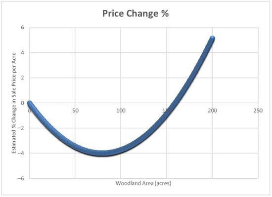
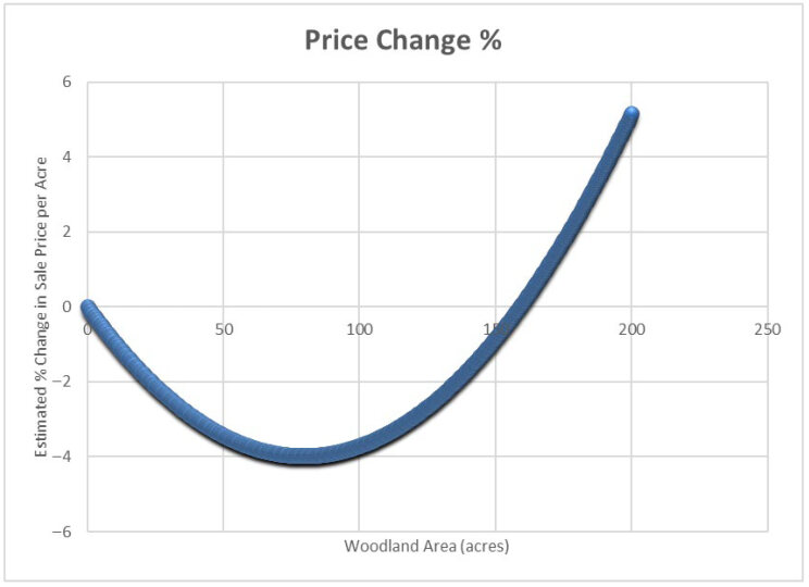
Graphically this is demonstrated in Figure 1, noting that the Woodac variable is not statistically significant and is therefore for illustration purposes only. The turning point is approximately 80 acres (32 hectares). The mean woodland area (10.23 acres/0.4 hectares) within the dataset is well below the estimated turning point, meaning that for most properties, woodland likely has a negative impact on price per acre. Only a small fraction of properties would have enough woodland for the effect to turn positive (closer to 80 acres or more).

Figure 1. Illustrative relationship between land price change and woodland area.

The mixed significance of these variables implies that the impact of woodland on land prices is nuanced. One interpretation is that a small amount of woodland may not be viewed as particularly beneficial, potentially because it reduces the usable agricultural area. However, as woodland cover increases, it may become an attractive feature for specific buyers, such as those interested in conservation, recreation, or diversified land use, thereby exerting a positive effect on price. This nonlinear relationship highlights the importance of considering the context in which woodland exists, as its valuation likely depends on factors such as land use type, property size, location, and buyer preferences.

6. Conclusions

This study focuses on the interrelationship between land values and woodland planting using a HPM approach. The analysis is grounded in past research on the economic, environmental, and policy dimensions of tree planting in agricultural landscapes. While trees offer well-documented benefits such as carbon sequestration, biodiversity enhancement, and improved farm resilience, their impact on land values remains complex and context dependent.

Through a review of existing HPM studies, the paper highlights key factors influencing agricultural land values, including soil quality, proximity to markets, infrastructure, and the presence of woodland. Based on this literature review we frame three hypotheses that we test in the empirical analysis, namely:

• Location, type of farm, farm infrastructure, land parcel size, and soil quality are important drivers of agricultural land values.
• The presence of woodland per se on a farm does not have a substantial or clear effect on price.
• Large woodland areas have a modest positive influence on farm sale prices above a certain threshold.

To test these hypotheses this study examines the interrelationship between land values and woodland planting using a HPM, analysing 1239 agricultural land transactions in England from 2014 to 2023. The dataset, provided by John Clegg & Co, includes key factors such as land area, soil quality, farm type, regional location, and the presence of farm infrastructure. The analysis aims to determine the extent to which woodland coverage influences agricultural land prices, while controlling for these economic and environmental variables. The research finds that Hypothesis 1, the location, type of farm, farm infrastructure, land parcel size, and soil quality are important drivers of agricultural land values is true. The findings also reveal that agricultural land values are shaped not only by productive capacity but also by amenity value, accessibility, and the potential for alternative land uses. Regional disparities, land quality classifications, and the presence of farm infrastructure significantly impact price variation. Additionally, broader market trends indicate rising land values in recent years, influenced by economic and policy factors.

With regard to Hypotheses 2 and 3 the empirical analysis of land transactions in England suggests that woodland area has a non-linear effect on land prices. The results indicate that the total woodland area on a property does not have a statistically significant effect on land prices in most cases. In other words, the existence of woodland on a farm does not significantly influence prices, confirming Hypothesis 2. However, larger woodland areas, above approximately 80 acres, show a modest positive impact on land values, implying a non-linear relationship in line with Hypothesis 3.

This suggests that while small-scale woodland integration may not meaningfully alter land prices, more extensive woodland coverage could become an attractive feature for certain buyers, particularly those interested in conservation, recreation, or alternative land use. A caveat to these findings is that the study does not consider or control for the spatial spread of trees in a farm. In addition, there are a range of data constraints on location and lack of planting data, plus an absence of behavioural variables that limit the robustness of the results. These are areas for future research, together with the ownership of land.

The results of this study suggest that the integration of woodland into agricultural landscapes requires careful consideration of economic incentives, policy support, and landowner perceptions. While tree planting contributes to environmental sustainability, its impact on land values is nuanced. Small-scale woodland integration may not substantially affect land prices, whereas larger woodland areas may enhance value in certain contexts.

Policymakers aiming to promote afforestation must recognise the trade-offs between traditional agricultural land use and woodland expansion. Incentive structures, regulatory frameworks, and land market dynamics all play crucial roles in shaping landowner decisions. Our research, in particular, suggests that there is an 80-acre threshold beyond which tree planting becomes viable and so incentives should be designed to apply to larger farms and be sufficient to enable this quantum to be achieved. Future research should explore the role of buyer motivations, geospatial factors, and the long-term financial returns of woodland planting. By refining economic models and integrating spatial data, a more comprehensive understanding of the economic implications of tree planting can be achieved, guiding strategies for sustainable land use and rural development.

References

- Westaway, S.; Grange, I.; Smith, J.; Smith, L.G. Meeting tree planting targets on the UK’s path to net-zero: A review of lessons learnt from 100 years of land use policies. Land Use Policy 2023, 125, 106502. [Google Scholar] [CrossRef] [Scilit]
- Read, D.; Freer-Smith, P.; Morison, J.; Hanely, N.; West, C.; Snowdon, P. Combating Climate Change: A Role for UK Forests. An Assessment of the Potential of the UK’s Trees and Woodlands to Migrate and Adapt to Climate Change; The Stationary Office: Edinburgh, UK, 2009. [Google Scholar]
- Cole, I.J.; Kleijn, D.; Dicks, L.V.; Stout, J.C.; Potts, S.G.; Albrecht, M.; Balzan, M.V.; Bartomeus, I.; Bebeli, P.J.; Bevk, D.; et al. A critical analysis of the potential for EU Common Agricultural Policy measures to support wild pollinators on farmland. J. Appl. Ecol. 2020, 57, 681–694. [Google Scholar] [CrossRef] [Scilit]
- Jose, S. Agroforestry for ecosystem services and environmental benefits: An overview. Agroforest Syst. 2009, 76, 1–10. [Google Scholar] [CrossRef] [Scilit]
- Torralba, M.; Fagerholm, N.; Burgess, P.; Moreno, G. Do European agroforestry systems enhance biodiversity and ecosystem services? A meta-analysis. Agric. Ecosyst. Environ. 2016, 230, 150–161. [Google Scholar] [CrossRef] [Scilit]
- Tsonkova, P.; Böhm, C.; Quinkenstein, A.; Freese, D. Ecological benefits provided by alley cropping systems for production of woody biomass in the temperate region: A review. Agroforest Syst. 2012, 85, 133–152. [Google Scholar] [CrossRef] [Scilit]
- Staddon, P.; Urquhart, J.; Mills, J.; Goodenough, A.; Powell, J.; Vigani, M.; Simmonds, P.; Rowe, E. Encouraging Woodland Creation, Regeneration and Tree Planting on Agricultural Land: A Literature Review NEER020; Countryside and Community Research Institute report to Natural England; Natural England: York, UK, 2021. [Google Scholar]
- Lawson, G.; Curran, E.; McAdam, J.; Strachan, M.; Pagella, T.; Smith, J. Policies to Encourage Trees on Farms in the UK and Ireland: June 2017 Update; Farm Woodland Forum: Aberdeen, UK, 2017; Available online: https://www.agroforestry.ac.uk/sites/www.agroforestry.ac.uk/files/2024-12/Lawson%20et%20al%202017.pdf (accessed on 4 February 2026).
- Committee on Climate Change. Reducing UK Emissions: 2020 Progress Report to Parliament; CCC: London, UK, 2020. [Google Scholar]
- Europe Economics. The Economic Benefits of Woodland; Woodlands Trust: London, UK, 2017. [Google Scholar]
- Marais, Z.E.; Baker, T.P.; O’Grady, A.P.; England, J.R.; Tinch, D.; Hunt, M.A. A natural capital approach to agroforestry decision-making at the farm scale. Forests 2019, 10, 980. [Google Scholar] [CrossRef] [Scilit]
- Ciaian, P.; Baldoni, E.; Kancs, d’.A.; Drabik, D. The capitalization of agricultural subsidies into land prices. Annu. Rev. Resour. Econ. 2021, 13, 17–38. [Google Scholar] [CrossRef] [Scilit]
- Feliciano, D.; Hunter, C.; Slee, B.; Smith, P. Climate change mitigation options in the rural land use sector: Stakeholders’ perspectives on barriers, enablers and the role of policy in North East Scotland. Environ. Sci. Policy 2014, 44, 26–28. [Google Scholar] [CrossRef] [Scilit]
- Ricardo, D. On the Principles of Political Economy and Taxation; Murray: London, UK, 1817. [Google Scholar]
- Lancaster, K.J. A new approach to consumer theory. J. Political Econ. 1966, 74, 132–157. [Google Scholar] [CrossRef] [Scilit]
- Rosen, S. Hedonic prices and implicit markets: Product differentiation in perfect competition. J. Political Econ. 1974, 82, 34–55. [Google Scholar] [CrossRef] [Scilit]
- Amirnejad, H.; Khalilian, S.; Assareh, M.; Ahmadian, M. Estimating the existence value of north forests of Iran by using a contingent valuation method. Ecol. Econ. 2006, 58, 665–675. [Google Scholar] [CrossRef] [Scilit]
- Weller, P.; Elsasser, P. Preferences for forest structural attributes in Germany—Evidence from a choice experiment. For. Policy Econ. 2018, 93, 1–9. [Google Scholar] [CrossRef] [Scilit]
- Haas, G.C. Sale Prices as a Basis for Farmland Appraisal; Bulletin 9 Agricultural Experiment Station; University of Minnesota: St Paul, MN, USA, 1922. [Google Scholar]
- Wallace, H.A. Comparative farm-land values in Iowa. J. Land Public Util. Econ. 1926, 2, 385–392. [Google Scholar] [CrossRef] [Scilit]
- Tempesta, T.; Foscolo, I.; Nardin, N.; Trentin, G. Farmland value in the “Conegliano Valdobbiadene Prosecco Superiore PGDO” area. An application of the hedonic pricing method. Aestimum 2021, 78, 5–33. [Google Scholar] [CrossRef] [Scilit]
- Khalid, H. Spatial heterogeneity and spatial bias analyses in hedonic price models: Some practical considerations. Bull. Geogr. Socio–Econ. Ser. 2015, 28, 113–129. [Google Scholar] [CrossRef] [Scilit]
- Chicoine, D.L. Farmland values at the urban fringe: An analysis of sale prices. Land Econ. 1981, 57, 353–362. [Google Scholar] [CrossRef] [Scilit]
- King, D.A.; Sinden, J.A. Influence of soil conservation on farmland values. Land Econ. 1988, 64, 242–255. [Google Scholar] [CrossRef] [Scilit]
- Palmquist, R.; Danielson, L. A hedonic study of the effects of erosion control and drainage on farmland values. Am. J. Agric. Econ. 1989, 71, 55–62. [Google Scholar] [CrossRef] [Scilit]
- Roka, F.M.; Palmquist, R.B. Examining the use of national databases in a hedonic analysis of regional farmland values. Am. J. Agric. Econ. 1997, 79, 1651–1656. [Google Scholar] [CrossRef] [Scilit]
- Bastian, C.T.; McLeod, D.M.; Germino, M.J.; Reiners, W.A.; Blasko, B.J. Environmental amenities and agricultural land values: A hedonic model using geographic information systems data. Ecol. Econ. 2002, 40, 337–349. [Google Scholar] [CrossRef] [Scilit]
- Lovell, S.; Lynch, L. Hedonic Price Analysis of Easement Payments in Agricultural Preservation Orders, WP02-13; Department of Agricultural and Resource Economics, University of Maryland: Baltimore, MD, USA, 2002. [Google Scholar]
- Tsoodle, L.J.; Golden, B.B.; Featherstone, A.M. Factors influencing Kansas agricultural farmland values. Land Econ. 2006, 82, 124–139. [Google Scholar] [CrossRef] [Scilit]
- Cotteleer, G.; Gardehroek, C.; Luijt, J. Market power in a GIS-based hedonic price model of local farmland markets. Land Econ. 2008, 84, 573–592. [Google Scholar] [CrossRef] [Scilit]
- Cotteleer, G.; van Kooten, G.C. Expert opinion versus actual transaction evidence in the valuation of non-market amenities. Econ. Model. 2012, 29, 32–40. [Google Scholar] [CrossRef] [Scilit]
- Ma, J.; Swinton, A. Hedonic valuation of farmland using sale prices versus appraised values. Land Econ. 2012, 88, 1–15. [Google Scholar] [CrossRef] [Scilit]
- Borchers, A.; Ifft, J.; Kuethe, T. Linking the price of agricultural land use values and amenities. Am. J. Agric. Econ. 2014, 96, 1307–1320. [Google Scholar] [CrossRef] [Scilit]
- Khan, S.; Ali, G.; Shah, S.A.; Jan, A.U.; Jan, D.; Fayaz, M.A. Hedonic analysis of agricultural land prices in Pakistan Peshawar District. Asian J. Agric. Rural Dev. 2016, 6, 59–67. [Google Scholar] [CrossRef] [Scilit]
- Sheng, Y.; Jackson, T.; Lawson, K. Evaluating the benefits from transport infrastructure in agriculture: A hedonic analysis of farmland prices. Aust. J. Agric. Resour. Econ. 2018, 62, 237–255. [Google Scholar] [CrossRef] [Scilit]
- Bigelow, D.P.; Ifft, J.; Kuethe, T. Following the market? Hedonic farmland valuation using sales prices versus self-reported values. Land Econ. 2020, 96, 418–440. [Google Scholar] [CrossRef] [Scilit]
- Maddison, D.A. hedonic analysis of agricultural land prices in England and Wales. Eur. Rev. Agric. Econ. 2020, 27, 519–532. [Google Scholar] [CrossRef] [Scilit]
- Ritter, M.; Huttel, S.; Odening, M.; Seifert, S. Revisiting the relationship between land price and parcel size in agriculture. Land Use Policy 2020, 97, 104771. [Google Scholar] [CrossRef] [Scilit]
- Clapp, J.M.; Giaccotto, C. Estimating price indices for residential property: A comparison of repeat sales and assessed value methods. J. Am. Stat. Assoc. 1992, 87, 300–306. [Google Scholar] [CrossRef]
- Cotteleer, G.; Stobbe, T.; van Kooten, G.C. Bayesian model averaging in the context of spatial hedonic pricing; An application to farmland values. J. Reg. Sci. 2011, 51, 540–557. [Google Scholar] [CrossRef] [Scilit]
- Jones, C.; Leishman, C.; Watkins, C. Structural change in a local urban housing market. Environ. Plan. A 2003, 35, 1315–1326. [Google Scholar] [CrossRef] [Scilit]
- Anderson, L.M.; Cordell, H.K. Influence of trees on residential property values in Athens, Georgia (U.S.A.): A survey based on actual sales prices. Landsc. Urban Plan. 1988, 15, 153–164. [Google Scholar] [CrossRef] [Scilit]
- Tyrvainen, L. The amenity value of the urban forest: An application of the hedonic pricing method. Landsc. Urban Plan. 1997, 37, 211–222. [Google Scholar] [CrossRef] [Scilit]
- Garrod, G.; Willis, K. The amenity value of woodland in Great Britain: A comparison of economic estimates. Environ. Resour. Econ. 1992, 2, 415–434. [Google Scholar] [CrossRef] [Scilit]
- Turner, R.; Newton, C.M.; Dennis, D.F. Economic relationships between parcel characteristics and price in the market for Vermont forestland. For. Sci. 1991, 37, 1150–1162. [Google Scholar] [CrossRef] [Scilit]
- Roos, A. Hedonic price function for forest land in Sweden. Can. J. For. Res. 1996, 26, 740–746. [Google Scholar] [CrossRef] [Scilit]
- Kennedy, G.A.; Vandeveer, L.R.; Henning, S.A.; Niu, H.; Deckard, D.L. Estimating tract value relationships in the north Louisiana timberland market. Southwest Econ. Rev. 2002, 26, 123–134. [Google Scholar]
- King, S.A.; Shreiner, D.F. Hedonic Estimation of Southeastern Oklahoma Forestland Prices. In Proceedings of the Southern Agricultural Economics Association Annual Meeting, Tulsa, OK, USA, 14–18 February 2004. [Google Scholar]
- Snyder, S.A.; Kilgore, M.A.; Hudson, R.; Donnay, J. Determinants of forest land prices in Northern Minnesota: A hedonic pricing approach. For. Sci. 2007, 53, 25–36. [Google Scholar] [CrossRef] [Scilit]
- Aronsson, T.; Carlen, O. The determinants of forest land price: An empirical analysis. Can. J. For. Res. 2020, 30, 589–595. [Google Scholar] [CrossRef]
- Zhang, D.; Meng, L.; Polyakov, M. Determinants of the prices of bare forestland and premerchantable timber stands: A spatial hedonic study. For. Sci. 2013, 59, 400–406. [Google Scholar] [CrossRef] [Scilit]
- Sundelin, T.; Högberg, J.; Lönnstedt, I. Determinants of the market price of forest estates: A statistical analysis. Scand. J. For. Res. 2015, 30, 547–557. [Google Scholar] [CrossRef] [Scilit]
- Gaca, R.; Zygmunt, R.; Gluszak, M. Comparative analysis of transaction prices and the values of forest properties in Poland. Forests 2020, 11, 1323. [Google Scholar] [CrossRef] [Scilit]
- Lautrup, M.; Panduro, T.E.; Olsen, J.V.; Pedersen, M.F.; Jacobsen, J.B. Is there more to trees than timber? Estimating the private amenity value of forests using a hedonic land model for combined agricultural properties. For. Policy Econ. 2023, 146, 102867. [Google Scholar] [CrossRef] [Scilit]
- Dubé, J.; Legros, D. Spatial econometrics and the hedonic pricing model: What about the temporal dimension? J. Prop. Res. 2014, 31, 333–359. [Google Scholar] [CrossRef] [Scilit]
- Sage, J.; Pace, R.K. Introduction to Spatial Econometrics; CRC Press: Boca Raton, FL, USA, 2009. [Google Scholar]
- Basu, S.; Thibodeau, T.G. Analysis of spatial autocorrelation in house prices. J. Real Estate Financ. Econ. 1998, 17, 61–85. [Google Scholar] [CrossRef] [Scilit]
- Savills. The Farmland Market, January 2025; Savills: London, UK, 2025. [Google Scholar]
Disclaimer/Publisher’s Note: The statements, opinions and data contained in all publications are solely those of the individual author(s) and contributor(s) and not of MDPI and/or the editor(s). MDPI and/or the editor(s) disclaim responsibility for any injury to people or property resulting from any ideas, methods, instructions or products referred to in the content. |
© 2026 by the authors. Licensee MDPI, Basel, Switzerland. This article is an open access article distributed under the terms and conditions of the Creative Commons Attribution (CC BY) license.