


Abstract
Ecological Security (ES) is an essential safeguard for regional sustainable development. Scientifically elucidating the multiscale evolution of ES patterns and their driving mechanisms is critical for ecological governance and conservation in Mountainous Urban Agglomerations (MUAs). Taking the central Yunnan Urban Agglomeration (CYUA) as a representative MUA, this study constructs a three-dimensional ES assessment framework integrating ecological health, ecological sensitivity, and ecological risk. By integrating ES slope-spectrum analysis with spatial autocorrelation, Geodetector, Multiscale Geographically Weighted Regression (MGWR), and machine learning, we analyze the spatiotemporal evolution of regional ES patterns and their driving mechanisms from a multiscale perspective. Results show that from 2000 to 2020, ES in the CYUA exhibited an overall improving trend with clear scale dependency. At the micro-scale, urban expansion intensified ecological fragmentation, whereas at the macro-scale, regional integration under policy guidance was evident. ES shows significant differentiation along slope gradients, forming a typical pattern of “low-slope–high-risk and high-slope–high-security,” with the 10–25° interval identified as a “conflict front” between ecological conservation and urban development, facing elevated degradation risks. Human Activity Intensity (HAI) is the dominant driver of ES spatial differentiation, with a critical pressure threshold of 0.29, and exhibits significant nonlinear interactive effects with slope and NDVI, with q-values exceeding 0.6. Overall, this study reveals complex human–environment interactions in MUAs and provides scientific evidence for balancing topographic constraints with urbanization, optimizing territorial spatial patterns, and promoting coordinated development of ecological conservation and high-quality urbanization.
1. Introduction
Ecological Security (ES) constitutes the fundamental basis of regional sustainable development [1], reflecting the integrated capacity of ecosystems to support socioeconomic activities while resisting external disturbances and maintaining structural integrity and functional stability [2,3,4]. With the acceleration of urbanization, high-intensity human activities have continuously reshaped land-cover patterns and ecological processes, triggering a series of challenges such as habitat fragmentation, degradation of ecosystem services, and declining system stability [5,6,7]. When cumulative anthropogenic disturbances exceed the resilience thresholds of ecosystems, not only are regional agricultural and industrial production rigidly constrained, but ecological security barriers may also experience systemic destabilization, posing long-term threats to human well-being [8]. Consequently, under rapid urbanization, scientifically assessing ES patterns and identifying their key threat mechanisms have become central issues in global sustainability research.
Compared with plains, plateau and mountainous ecosystems are constrained by complex topographic conditions, resulting in fundamentally different human–environment coupling logics in ES evolution. Topographic relief not only defines the physical upper limits of environmental carrying capacity but also profoundly shapes urban expansion pathways and the spatial organization of ecological processes. Such regions commonly face a structural contradiction: land suitable for urban construction is extremely scarce, whereas rigid demands for socioeconomic development continue to increase. Under this context, high-intensity human activities inevitably break through topographic constraints and expand toward steeper, ecologically sensitive mountainous margins, forming a typical “upslope urban expansion” pattern. This process leads to substantial spatial overlap between urban development land and ecological barrier functional zones, exacerbating soil erosion, habitat fragmentation, and ecological connectivity degradation, and causing ES risks to become highly concentrated along specific topographic gradients.
As a representative mountainous urban agglomeration in Southwestern China, the Central Yunnan Urban Agglomeration (CYUA) vividly embodies this human–land conflict. On the one hand, constrained by a karst geological background, its ecosystems exhibit pronounced inherent vulnerability, characterized by shallow soil layers, discontinuous surface–subsurface hydrological systems, and limited ecological recovery capacity [9,10]. On the other hand, as a regional economic growth pole, rapid urbanization has generated strong tension with limited environmental capacity. The interaction between rigid geological constraints (e.g., shallow soils, high erosion susceptibility, and frequent geological hazards) and upslope urban expansion accelerates localized ecological degradation [11]. Through downslope hydrological connectivity, landscape fragmentation, and the spatial clustering of disturbed patches within administrative units, such site-specific degradation is more likely to propagate across space and accumulate into broader regional ES risks. The superposition of a “fragile natural background” and “high-intensity human disturbance” renders the CYUA a representative case for investigating ES evolution mechanisms in Mountainous Urban Agglomerations (MUAs).
Although substantial progress has been made in ES assessment, existing research paradigms remain insufficient for characterizing the complexity of mountainous ecosystems. Most studies rely on single logical frameworks, such as the Pressure–State–Response (PSR) model [7,12] or the Driver–Pressure–State–Impact–Response (DPSIR) framework [1], or emphasize specific indicator systems such as energy analysis [13] and ecological footprints [4,14]. These approaches tend to focus on individual dimensions of ecological security, while insufficiently integrating ecosystem health (e.g., vegetation condition and landscape organization), environmental sensitivity (e.g., topography, soil erosion, and climatic constraints), and risk stress (e.g., human interference and natural hazards) as an interacting system with explicit process linkages, which is particularly problematic in topographically constrained regions. In particular, terrain-induced sensitivity and geological background conditions—such as steep slope gradients and karst development—are often treated as static boundary constraints, rather than as conditioning factors that influence the ecological consequences of upslope urban expansion and human activity intensification [15]. In mountainous settings, fragile lithological conditions and slope instability can amplify the ecological impacts of land-use conversion and infrastructure construction, while in relatively stable terrains similar urban pressures may lead to weaker ES responses. This simplification limits the theoretical integration of natural background constraints with urbanization-driven risk processes, and makes it difficult to explain why ecological degradation and ES risks are disproportionately amplified or attenuated along specific topographic gradients in MUAs.
More critically, most existing studies are confined to static analyses at a single spatial scale [16,17], lacking systematic investigation into how ES patterns are transmitted, amplified, or attenuated across scales. Although recent studies have begun to compare ES patterns across grid, watershed, or administrative units [18,19,20], such analyses are often limited to descriptive comparisons of spatial patterns, with insufficient attention to the underlying process mechanisms of scale-dependent signal transformation. From a process perspective, ecological degradation often originates at fine spatial units (e.g., grid or slope segments) through localized land-use conversion or infrastructure expansion, but may be partially masked or diluted when aggregated to coarser administrative units due to spatial averaging effects [21,22]. Such aggregation can obscure high-risk hotspots in environmentally sensitive zones, while weakening the apparent influence of terrain- or geology-controlled processes at administrative scales. Consequently, single-scale perspectives disconnect micro-level physical–geographical processes from macro-level administrative governance units, limiting understanding of how localized ecological degradation evolves into regional ES risks, particularly in MUAs where strong topographic constraints coexist with administrative-scale aggregation [23].
Mechanistically, the evolution of ES patterns is essentially the result of nonlinear coupling between natural background conditions and anthropogenic disturbances. However, existing studies predominantly rely on traditional global linear regression models or simple correlation analyses to identify driving factors, while neglecting the spatial heterogeneity of these drivers across different geographic units [24,25,26]. As a result, locally critical characteristics are often obscured by global average effects. For example, the impacts of economic growth on ES frequently differ markedly in both direction and magnitude between urban core areas and ecological conservation zones [27,28]. More importantly, driving factors often exhibit complex synergistic enhancement effects, and the linear superposition of individual factors is insufficient to explain the amplified risks arising from interactions between natural constraints and anthropogenic pressures [29]. Different analytical methods vary in their ability to capture these mechanisms: global models are effective for identifying dominant drivers at the regional scale but are insensitive to local variability, whereas local models can reveal spatial heterogeneity but may overlook cross-scale consistency and interaction effects [30]. This limitation is particularly pronounced in MUAs, where human–environment relationships are highly sensitive [31]. Therefore, there remains a need for integrated analytical frameworks that can simultaneously identify dominant drivers, quantify interaction effects, and capture scale-dependent spatial heterogeneity of ES driving mechanisms.
In response to these challenges, this study takes the CYUA as the research object and develops an integrated ES assessment and driving mechanism analysis framework tailored for MUAs. The objectives are to: (1) construct a three-dimensional ES assessment framework integrating ecological health, ecological sensitivity, and ecological risk, and systematically characterize the spatiotemporal evolution of the Ecological Security Index (ESI) from 2000 to 2020; (2) introduce ES slope-spectrum analysis and multiscale spatial autocorrelation to reveal spatial heterogeneity in ES patterns and their differentiation along topographic gradients across multiple scales; and (3) integrate Geodetector and Multiscale Geographically Weighted Regression (MGWR) to quantitatively identify scale dependency, interaction effects, and critical thresholds of ES driving factors. By systematically elucidating the compound driving mechanisms arising from topographic constraints and anthropogenic pressures in MUAs, this study aims to provide scientific support for topography-based zonal regulation and ecological spatial optimization. The findings offer valuable references for promoting coordinated development between ecological conservation and high-quality urbanization in the CYUA and other MUAs with similar environmental conditions.
2. Materials and Methods
2.1. Study Area
Situated within a core area of China’s Western Development Strategy, the CYUA encompasses 49 counties and major cities such as Kunming, Qujing, Yuxi, and Chuxiong (Figure 1). The region features highly diverse landforms and strong altitudinal gradients and is governed by a subtropical plateau monsoon climate with abundant, seasonally concentrated precipitation. These geomorphic and climatic conditions support rich vegetation, making the area a key water conservation zone and a global biodiversity hotspot. Wetland ecosystems formed by plateau lakes and major river basins further reinforce the area’s role as an ES barrier in Southwest China.
Figure 1.
The location, elevation and land cover in CYUA.
However, rapid economic expansion—characterized by population growth, urbanization, and intensified industrial activity—has imposed increasing ecological pressures, resulting in accumulating risks to ecosystem structure and function [32]. This underscores the urgent need for systematic assessment and enhancement of the region’s self-regulation capacity, ecological resilience, and sustainable development potential.
2.2. Data Sources
In this study, the data used include topography, climate, river networks, soil erodibility, NDVI, LUCC, GDP, population and road networks. To ensure spatial consistency, all data were resampled to unified 30 m resolution using the nearest-neighbor method prior to indicator calculation. Based on the 30 m grids, each ES-related indicator was calculated separately within township and county administrative units. Subsequently, ES sub-indices and the overall ESI were constructed independently at the township and county scales. The primary data employed in this research are summarized in Table 1 and Supplementary Material S1.
Table 1.
Basic information and applications of the data.
2.3. Methods
The methodological framework of this study is structured as follows (Figure 2). First, by collecting fundamental geospatial datasets, ESI was constructed based on three core dimensions: ecological health, ecological sensitivity, and ecological risk. Specifically, ecological health was characterized by indicators of vigor, organization, and resilience; ecological sensitivity was defined to reflect the susceptibility of ecosystems to terrain, climatic, soil, and hydrological conditions; and ecological risk was represented by human disturbance, natural hazards, and landscape ecology–related risks. Subsequently, the Analytic hierarchy process (AHP) and entropy weight method were integrated to derive the comprehensive weights of ESI.
Figure 2.
Technical framework.
The ESI was then analyzed at multiple spatial scales, including grid, town, and county scales. Next, the temporal and spatial patterns of ESI and its variation across slope gradients were examined using transition matrices and ecological security slope spectrum. Spatial autocorrelation analysis was applied to evaluate the clustering characteristics of ESI. Following this, Geodetector was used to identify the dominant driving factors influencing ESI distribution. Finally, using the Exploratory Regression Analysis (ERA) to determine the optimal combination of driving variables, the spatial heterogeneity of ESI drivers was assessed through MGWR model.
2.3.1. Ecological Security Index (ESI) Framework
ES is manifested in the structural integrity and functional soundness of ecosystems [34], characterized by their resilience to multiple risks such as natural disasters and human interference. A secure ecosystem maintains long-term self-regulation and dynamic equilibrium. Thus, we construct a multidimensional ES assessment framework based on ecological health, sensitivity, and risk. ES is manifested in the complete structure of the ecosystem, sound functions, the resilience to resist multiple risks such as natural disasters and the impact of human activities, and the ability to maintain self-repair and dynamic balance for a long time. This study constructs a multi-dimensional ESI assessment framework from the aspects of ecosystem health, sensitivity and risk. Ecological health focuses on the internal structure and functions of the ecosystem, reflecting its vitality in withstanding environmental disturbances, sustaining continuity, and enabling rapid recovery [35]. Ecological sensitivity refers to the ecosystem’s vulnerability and probability of degradation or imbalance when subjected to external negative impacts, particularly from human activities [16,36]. Ecological risk centers on external threats faced by the ecosystem, especially those arising from human production, livelihood activities, and resource exploitation [37]. It emphasizes the likelihood and extent to which these risk factors may negatively affect ecosystem structure, function, and service provision (Table 2).
Table 2.
ESI framework.
Ecological health assesses internal stability, ecological sensitivity reveals the degree of system fragility, and ecological risk targets external pressures. The integration of these three dimensions enables a comprehensive, bidirectional evaluation of ES—from internal vulnerability to external threats—thereby enhancing the completeness, accuracy, and effectiveness of ecosystem security assessments.
In ecological assessment, ecosystem vigor, structural organization, and resilience are frequently used to evaluate ecological health [38]. In this study, NDVI was used to represent vigor; structural organization was quantified through landscape indices calculated using Fragstats v4.2 software; and resilience was assessed using habitat quality generated by the InVEST v3.14.3 model [39,40,41]. CYUA, characterized as a typical plateau karst region, features complex natural topography. To reflect ecological sensitivity to environmental conditions, we selected slope, soil erodibility, aridity index, and distance to rivers as representative indicators of the natural geographic environment [16,42,43]. In terms of ecological risk, HAI was used to quantify human interference; geological hazard density was used to capture the impact of natural disasters on ecosystem stability; and Landscape Ecological Risk (LER) was used to represent the role of landscape patterns in ecological processes [38,44,45]. The specific formulas for calculating each index are provided in the Supplementary Material S2.
ESI was calculated using a linear weighted composite method, expressed mathematically as the following Formula (1):
where denotes the comprehensive weight of indicator , and represents the standardized value of indicator .
To reduce the uncertainty and potential bias associated with a single weighting method, a combined weighting strategy integrating the AHP and the entropy weight method was adopted. Specifically, AHP was used to determine indicator weights based on expert judgment and theoretical understanding of ecosystem structure and functioning, thereby reflecting the relative importance of indicators from a subjective perspective. In contrast, the entropy weight method derives weights according to the degree of variation and information entropy of each indicator, emphasizing the objective contribution of indicators based on their data distribution. The comprehensive weight of each indicator was computed as the arithmetic mean of the two weights, expressed as the following Formula (2):
where and denote the weights derived from the AHP and entropy methods, respectively, and represents the final comprehensive weight used in the ESI calculation.
This integrated weighting scheme balances expert knowledge and data-driven information by assigning them equal influence, and has been widely applied in ecological and environmental assessment studies to reduce weighting uncertainty and improve the robustness and interpretability of composite indices [46,47]. The final integrated weights of all ESI indicators are presented in Supplementary Material S3 and summarized in Table S5. All indicators were normalized using dimensionless transformation. The final ESI values were classified into five categories—lowest safe, low safe, moderate safe, high safe and highest safe—based on the natural breaks classification method [48]. To ensure comparability across time, the classification thresholds were defined using the 2000 ESI grading standard.
2.3.2. ESI Slope Spectrum
Based on the slope data and the spatial distribution of ESI, we use statistical analysis of ESI across different slope intervals at 1-degree increments. A topographic slope-spectrum curve and slope-spectrum curves [49] for each ESI level are constructed to explore the relationship between terrain gradients and ESI. The Formulas (3) and (4) are given by:
where denotes the frequency of land area at slope interval relative to the total land area of the study region; indicates the frequency of land area at slope within a specific ESI level relative to the total area of that ESI; and represent the land area at slope for the entire study area and for a given ESI, respectively; and are the total land area of the study region and the total land area of the respective ESI level.
2.3.3. Spatial Autocorrelation Analysis
The global Moran’s I and local Moran’s I indices are commonly used to measure the spatial aggregation of unit attribute values and the overall spatial autocorrelation, as well as the extent to which nearby variables influence each other’s spatial distribution [16,50]. Typically, Moran’s I index ranges from −1 to 1, with larger absolute values indicating stronger correlation. The LISA value reflects the spatial clustering of a specific point within the spatial resource and captures the local spatial correlation characteristics of ESI. The GeoDa v1.22 software was used to analyze both the overall spatial autocorrelation and the local spatial association of the ESI.
2.3.4. Geodetector
The Geodetector is a statistical tool used to analyze the spatial heterogeneity of a target variable and reveal its driving factors [51]. In the Geodetector model, the factor detector uses the q-value to measure the explanatory power of each independent variable X on the dependent variable Y, allowing for the assessment of whether there is significant spatial consistency between the independent and dependent variables. The q-value ranges from 0 to 1, where a higher q-value indicates stronger explanatory power of the influencing variable [52]. The Formula (5) is given by:
where is the number of categories of influence in the study area; and are the total number of observation units in the entire study area and in the layer, respectively; and represent the variance of the dependent variable in the entire study area and in the layer, respectively.
Furthermore, the interaction detector is used to identify the interaction between two independent variables and their combined effect on the dependent variable (Table 3). This tool assesses whether the joint effect of two factors enhances or weakens their explanatory power on the dependent variable, thereby evaluating whether the driving factors increase or decrease the explanatory power of spatial differentiation in ESI.
Table 3.
Types of factor interactions.
2.3.5. Multiscale Geographically Weighted Regression
MGWR can reveal the multiscale effects and spatial heterogeneity, reflecting the relationship between the dependent variable and independent variables. The correlation between each factor and ESI is not constant across space; each regression coefficient is dependent on local regressions and has its own specific bandwidth, which distinguishes it from the traditional Geographically Weighted Regression (GWR) model [53]. In this study, MGWR is used to reflect the degree of influence various factors have on the ESI.
3. Results
3.1. Spatiotemporal Evolution of ESI
Figure 3 illustrates the spatial distribution patterns of the ESI in 2000, 2010, and 2020. The results indicate that ES in the CYUA exhibits pronounced spatial heterogeneity and clear scale dependency.
Figure 3.
The ESI spatial distribution. The spatial distribution and proportion of ESI. (a)–(d) represent the spatial distribution of ESI in 2000, 2010, 2020, and the average period respectively. (e) shows the proportion of ESI levels corresponding to the three scales.
Overall, the ES pattern is characterized by a “high-periphery–low-core” configuration. Areas with high and highest ES are mainly concentrated in the continuous mountainous regions in the western and northern parts of the CYUA, as well as in key water conservation zones, where favorable natural background conditions support relatively intact ecosystem structures. In contrast, low-ES areas display a distinct point–axis clustering pattern, highly concentrated in the core urban area of Kunming and along major transportation corridors. The spatial distribution of these low-value areas shows a high degree of consistency with high-density built-up land, indicating that intensive human development exerts substantial pressure on the local ecological environment.
With increasing spatial scale, the fragmentation of ES patterns gradually decreases, forming a “core–periphery” gradient structure with the Kunming metropolitan area as a low-value center and progressively higher ESI levels toward the periphery. Peripheral counties, characterized by better natural vegetation cover and relatively lower development intensity, generally maintain higher ESI values, whereas counties with low ES levels are fewer in number and spatially adjacent to the main directions of urban expansion.
From a temporal perspective, the hierarchical structure of ESI remains relatively stable across scales. Quantitative statistics show that areas with moderate and higher ES levels consistently dominate, particularly at the county scale, where the combined proportion of moderately high and very high ES areas exceeds 70%. This indicates that, at the regional scale, the overall ecological foundation of the CYUA has remained generally stable.
Based on the ES level transition matrix analysis (Figure 4), the dynamic trajectories of ESI evolution are further revealed. During the period from 2000 to 2010, regional ES exhibited an overall improving trend, primarily characterized by transitions from medium ES to higher security levels, accounting for 69.37% of the total transitions. However, during 2010–2020, this trend showed notable fluctuations, with partial areas experiencing grade regression, as reflected by a significant increase in transitions from moderate ES to lower security levels (55.82%). These areas are mainly concentrated along urban fringes and emerging development zones, indicating that rapid urbanization and abrupt land-use changes have intensified local ecological risks, thereby partially offsetting the positive effects of natural recovery. Despite these localized disturbances, the net effect over the entire period from 2000 to 2020 still indicates an overall improvement in ecological stability, suggesting that regional ecological governance measures have played a positive role.
Figure 4.
Transition directions of ESI levels.
3.2. Differentiation of Ecological Security (ES) Patterns and Identification of Critical Thresholds Along Slope Gradients
To reveal the constraining effects of topographic gradients on ES patterns, slope was extracted at 1° intervals, and an ES slope-spectrum analysis framework was constructed by overlaying slope frequency distributions with ES grade frequencies. The results show that the study area is dominated by low-to-moderate slopes, with the 0–30° range accounting for 88.75% of the total area. Among them, the 5–15° interval occupies the largest proportion (31.69%), exhibiting a clear unimodal distribution (Figure 5).
Figure 5.
Topographic slope spectrum and ESI slope spectrum.
The slope-spectrum analysis further reveals pronounced features of both “polarization” and “dynamic competition” in ES patterns along topographic gradients. Specifically, the lowest ES grade shows strong spatial clustering across slope intervals and exhibits a typical bimodal structure. The first peak occurs in extremely flat areas (0–2°), where the curve displays a steep, eruptive pattern with a frequency as high as 12%, indicating the overwhelming dominance of urban cores and high-intensity development zones that effectively lock this interval into the lowest ES state. The second peak emerges in the gentle slope zone of 10–20°, characterized by a broad uplift. This interval corresponds to areas with relatively abundant land resources and serves as the primary carrier of agricultural reclamation and urban fringe expansion, leading to secondary clustering of low ES levels.
In contrast to the rigid constraints observed at low slopes, mid- to high-slope areas exhibit a positive trend of ecological recovery. A comparison of slope-spectrum curves between 2000 and 2020 shows that within the 15–30° interval, the curve representing the highest ES grade shifts from being lower than that of the high ES grade in 2000 to forming a pronounced peak and overtaking it by 2020. This transition indicates that over the past two decades, while low-slope areas have remained under sustained anthropogenic pressure, ecosystem quality in mid- to high-slope areas has evolved from a “relatively good” to an “optimal” state, reflecting the significant effectiveness of reforestation programs and ecological barrier protection policies at specific topographic gradients.
By examining the intersection patterns among ES grade curves, critical topographic control nodes can be further identified. Within the 0–12° interval, the frequency of low ES grades is overwhelmingly dominant. Beyond 12°, however, the frequency curve of high ES grades surpasses that of low ES grades, indicating that natural recovery capacity and ecosystem stability begin to prevail.
Notably, the transitional slope zone of 10–25° constitutes a “frontline” of competition between ecological degradation and construction expansion. This interval is not only a mixed zone where ES grade curves intersect intensively, but also the most temporally dynamic and sensitive area. Analysis of changes from 2000 to 2020 reveals that as development in flat areas (0–10°) has approached saturation, low ES areas have expanded markedly toward the 10–25° hilly and piedmont zones. The increasing proportion of low ES grades and the retreat of high ES grades within this interval clearly delineate an upward-shifting conflict frontier.
This upward shift is closely associated with the combined effects of land-use regulation constraints and development spillover processes. In the CYUA, strict protection of basic farmland and ecological redlines in flat valley areas has progressively limited the availability of construction land in low-slope zones, indirectly redirecting urban expansion, infrastructure development, and associated human activities toward adjacent hilly and piedmont areas with moderate slopes. At the same time, transportation infrastructure construction—such as hillside road networks, industrial access roads, and slope-cutting projects—has lowered the development threshold of mid-slope areas, intensifying land-use conversion and landscape fragmentation within the 10–25° interval.
Under these conditions, the 10–25° slope zone functions as a spatial buffer where policy-induced constraints on flatland development intersect with growing urban land demand, making it particularly susceptible to the accumulation of human disturbance and ecological risk. This process explains why the conflict frontier has shifted upward rather than remaining confined to traditional low-slope urban core. This indicates that urbanization is breaking through traditional flatland constraints and advancing into mid-slope areas with higher ecological sensitivity, substantially increasing ecological vulnerability within this gradient.
Although high-slope areas have generally maintained relatively stable ES levels, the 10–25° transitional zone has emerged as the most intense spatial arena of human–environment conflict in both the present and the future. This slope interval should therefore be prioritized as a critical ecological control boundary, with strict limitations imposed on the unregulated expansion of construction land from plains toward mountainous foothills.
3.3. Spatial Clustering Characteristics and Scale Effects of ES Patterns
To examine the spatial dependence of ES patterns and their responses to observation scale, global Moran’s I was calculated at three scales—grid, township, and county (Figure 6). The results show that Moran’s I values at all scales are positive and statistically significant, confirming strong positive spatial autocorrelation in ES patterns across the CYUA.
Figure 6.
Moran’s I scatter plot of ESI.
At the grid scale, Moran’s I remains at a high level above 0.73, indicating a high degree of local spatial continuity in ecosystem conditions. Notably, this index exhibits a slight downward trend during the study period, decreasing from 0.769 to 0.732. This subtle decline suggests that the embedding of urbanized patches has begun to disrupt local ecological connectivity, with early signs of spatial fragmentation emerging. As the observation scale shifts to the township and county levels, spatial dependence naturally weakens with the enlargement of spatial units. However, in contrast to the declining trend observed at the grid scale, Moran’s I at the county level shows an opposite increasing trend from 2000 to 2020, rising from 0.318 to 0.393. This inverse evolution reflects a macro-scale spatial integration process, indicating that under the guidance of regional integration policies and the Major Function-Oriented Zoning (MFOZ) strategy, adjacent counties have increasingly coordinated their approaches to ecological protection and development. As a result, ecological conservation zones and key development areas have become more spatially clustered, enhancing the structural organization of ES patterns at the macro scale.
Given that global statistics are insufficient to reveal the locational characteristics of spatial dependence, Local Indicators of Spatial Association (LISA) were further employed to identify hot–cold spot patterns of ES (Figure 7). The results show that significant areas are dominated by homogeneous clustering of “High–High” and “Low–Low” types, whereas spatial outliers (High–Low or Low–High) are rare, indicating a pronounced spatial polarization of ES levels.
Figure 7.
LISA results of ESI.
In terms of spatial configuration, the study area exhibits a clear “low-core–high-periphery” binary structure. “Low–Low” clusters are highly concentrated in the central urbanized zone centered on Kunming. As the economic and population core of the CYUA, this area has been subjected to sustained ecological pressure from high-intensity land development and rapid expansion of impervious surfaces, resulting in a stable low-ES lock-in and forming a regional “central collapse zone” of ecological security. In contrast, “High–High” clusters are mainly distributed in a ring-like pattern along the margins of the Chuxiong Basin in the west and the mountainous areas in the east. These regions are predominantly high-altitude areas covered by forests and grasslands, where human disturbance is relatively limited due to topographic barriers. Benefiting from the implementation of policies such as natural forest protection, they have maintained consistently high ES levels, constituting robust ecological barriers along the periphery of the urban agglomeration. As the observation scale shifts from the grid to the county level, this “core–periphery” differentiation becomes increasingly pronounced and spatial boundaries tend to solidify, revealing a marked internal spatial discontinuity in development intensity and conservation effectiveness across the region.
3.4. Multiscale Driving Mechanisms of ES Pattern
Based on factor detection and interaction detection using the Geodetector, this study systematically reveals the composite driving effects of the natural geographical environment and socioeconomic activities on the ES pattern. The factor detection results (Figure 8a) show pronounced scale-dependent heterogeneity in the explanatory power (q values) of the driving factors. HAI (X9) and NDVI (X6) rank among the most influential factors, indicating that local ES is primarily regulated by surface vegetation cover and the intensity of anthropogenic disturbance. However, as the observation scale extends to the township and county levels, the explanatory power of topographic factors such as slope increases markedly at the township scale, reflecting the constraining role of mountainous terrain on peri-urban development and agricultural layout. At the county scale, distance to roads (X10) and HAI (X9) replace natural factors as the dominant drivers, suggesting that infrastructure configuration and regional development intensity are the core forces shaping the macro-scale ES pattern.
Figure 8.
Geodetector results: factor detector (a) and interaction factor (b–d). Note: ▼ indicates nonlinear enhancement. ▲ indicates bivariate enhancement. Variables X1 to X11 represent: elevation (X1), slope (X2), temperature (X3), precipitation (X4), potential evapotranspiration (X5), NDVI (X6), GDP (X7), population (X8), HAI (X9), distance to roads (X10), and distance to railways (X11).
Interaction detection further indicates (Figure 8b–d) that all pairs of factors exhibit either nonlinear enhancement or bivariate enhancement, with no independent or weakening effects observed. At the grid scale, the interaction between HAI (X9) and NDVI (X6) is the most pronounced (q = 0.43), characterized by bivariate enhancement. This indicates a strong superposition effect between anthropogenic disturbance and vegetation background: in areas with fragile vegetation, human activities of equivalent intensity tend to trigger more severe ecological degradation.
Notably, the strength of interaction effects increases with spatial scale, and interaction types progressively shift from bivariate enhancement to nonlinear enhancement. At the county scale, the q values of multiple factor interactions exceed 0.6, with the synergistic effects between HAI (X9) and distance to railways (X11), as well as slope (X2), reaching their peaks. This implies that, at the macro level, high-intensity human development often spatially overlaps with specific transportation locations or terrain conditions, forming a composite stress mechanism of “natural background–infrastructure–human disturbance.”
Overall, the evolution of the ES pattern in CYUA is jointly driven by the rigid constraints of the natural environment and the plastic disturbances of human activities. In particular, HAI, attracted by gentle slopes and road networks, forms high-density clustering and interaction superposition along low-slope areas and transportation corridors, which constitutes the fundamental driver of sharp increases in localized ecological risk. These findings provide a scientific basis for formulating targeted ecological protection and spatial control strategies in mountainous urban regions.
3.5. The Spatial Heterogeneity of the Driving Factors
3.5.1. Optimal Combination of Driving Factors
After using the Geodetector to study the driving factors of the ESI, we further explored the spatial heterogeneity of the driving factors affecting ESI. First, after removing the collinear factors through ERA, the optimal combination of influential factors affecting ESI in the region was determined. The results show that Combination 1 has a high adjusted R2 value and a low AICc value, with VIF values below 7.5, indicating that there is no collinearity problem among the influencing factors (Table 4). Based on the principle of selecting influencing factors, this combination was identified as the optimal set of driving factors.
Table 4.
ERA results of driving factors.
3.5.2. Comparison Between GWR and MGWR Models
The GWR and MGWR models were then compared by determining the optimal combination of drivers through ERA. The results show that the AICc value of the MGWR model is smaller than that of the GWR model, while the Adjusted R2 value is larger for the MGWR model (Table 5). This indicates that the MGWR model significantly improves performance and is better able to explain the local variations in the driving factors. Beyond the improvement in overall model fit, the MGWR model reveals clearer spatial differentiation in the effects of individual driving factors, highlighting heterogeneous response patterns across geographic space that are not fully captured by the standard GWR model.
Table 5.
Comparison results of GWR and MGWR models.
3.5.3. Spatial Variation in Driving Factors Influence
Based on the MGWR model, we quantified the average effects of individual driving factors (Figure 9 and Supplementary Material S4), revealing pronounced spatial non-stationarity in the driving mechanisms of ES. The results indicate that the constraining effects of the natural background and the stress effects of human activities exhibit differentiated coupling patterns across geographic units.
Figure 9.
Spatial distribution and positive or negative proportions of regression coefficients for driving factors.
With respect to natural factors, topographic constraints show strong geomorphology-dependent characteristics. Elevation exerts a significantly strong negative effect in the high mountain–gorge regions of the eastern and southeastern study area (e.g., along the Jinsha River and deeply incised valleys), with coefficients generally lower than −0.7. These areas are characterized by extreme terrain relief, where high elevations are often associated with shallow soils and fragmented habitats, rendering ecosystems highly sensitive to elevation gradients. The negative effect of slope is more pervasive across the entire region, with extremely low coefficients (<−0.9) precisely corresponding to the margins of eastern karst faulted basins and karst hill landscapes. In these ecologically fragile zones, the combination of steep slopes and highly erodible calcareous soils makes the system particularly vulnerable to cultivation disturbances, readily triggering rocky desertification processes and thereby maximizing the negative constraining effect of slope on ES.
As a dominant positive driving factor, NDVI exhibits its strongest promoting effect in the contiguous forested areas of western mountain ranges such as the Ailao and Wuliang Mountains. However, in the hot–dry valley zones along the northern Jinsha River, the regression coefficients of NDVI are markedly lower, indicating that under the unique climatic habitats characterized by high temperatures and aridity, increases in vegetation cover alone are insufficient to fully offset the ecological stress induced by chronic water deficits.
Socioeconomic factors display a concentric, urban-centered pattern of stress. Strong negative impacts of population density are highly clustered along the “Kunming–Yuxi” core urban corridor (mean coefficient = −0.3934). Along this urbanization axis, intensive resource consumption and domestic pollution emissions associated with high population densities exert persistent compressive pressures on surrounding ecosystems. HAI is identified as the most destructive systemic pressure source, exhibiting consistently negative coefficients across the entire region (mean coefficient = −0.5186). The spatial centers of its lowest coefficients closely overlap with mineral exploitation zones and heavy industrial bases in areas such as Dongchuan, Anning, and Yimen. In these regions, mining-induced vegetation stripping, land degradation, and industrial land occupation impose high-intensity point-source disturbances on ES, significantly depressing the overall regional ES level.
These spatially differentiated coefficient patterns further demonstrate that the impacts of both natural constraints and human activities vary substantially across space, reinforcing the presence of strong spatial heterogeneity in ES driving mechanisms. These spatially heterogeneous mechanisms indicate that a uniform ecological governance model is unlikely to be effective. Future ecological spatial regulation should adopt a zoned management strategy: strict cropland-to-forest conversion and enclosure measures should be implemented in the eastern karst steep-slope regions to curb rocky desertification; drought-tolerant vegetation community restoration should be explored in hot–dry valley areas; and along the Kunming–Yuxi urban axis and in mining–industrial zones, priority should be given to promoting intensive use of construction land and mine ecological restoration to alleviate the cumulative pressures of human activities on the ecological foundation.
4. Discussion
4.1. Differences in the Driving Factors of ESI
Understanding the driving mechanisms of regional ES provides an essential theoretical basis for the formulation of regional ecological policies. Although the Geodetector and MGWR models have clarified the dominant driving factors and their spatial heterogeneity, these methods are primarily linear or semi-parametric and are limited in their ability to explicitly capture complex nonlinear responses and threshold effects. Both approaches are effective for identifying key drivers and spatial differentiation patterns, but they provide limited insight into nonlinear response trajectories at the variable level [54]. Therefore, we further introduce the XGBoost model combined with the SHAP interpretability framework to quantitatively identify the nonlinear contributions and critical thresholds of individual factors [55]. Compared with Geodetector, which focuses on factor explanatory power and interaction strength, and MGWR, which emphasizes spatial non-stationarity across geographic locations, the XGBoost–SHAP framework provides an alternative perspective by revealing the marginal contribution of each driver and its nonlinear response pattern across the entire feature space [56].
The global importance analysis (Figure 10) indicates that the evolution of the ES pattern is essentially a dynamic game between the maintenance of the natural background and disturbances induced by human activities. Among all drivers, HAI and NDVI occupy the most important negative and positive driving positions, respectively. This not only corroborates previous findings that vegetation cover is a dominant determinant of ecological health [57,58], but also highlights that in MUAs, high-intensity human activities have emerged as the primary pressure constraining ES.
Figure 10.
The importance of SHAP values of ES driver factors.
As a core manifestation of land-use change, HAI exerts a pronounced negative impact on the ESI by encroaching upon ecological space and exacerbating landscape fragmentation, which is consistent with earlier studies on the ecological effects of urbanization [59,60,61]. The SHAP dependence plots (Figure 11) further reveal the nonlinear nature of this impact: the negative effect of HAI on ESI does not increase at a constant rate. When HAI exceeds a threshold of 0.29, the corresponding SHAP values sharply decline into the negative range, indicating that once human disturbance surpasses this critical point, ecosystem functions face a risk of systemic degradation. This finding quantitatively explains the observed decline in ESI within economically developed areas [62] and provides an explicit quantitative benchmark for policy formulation. At the county and township scales, population density and HAI exhibit synergistic negative driving effects, reflecting the cumulative pressures of population agglomeration and economic growth on resource–environment carrying capacity [17]. Therefore, future spatial regulation should focus on resolving the structural contradiction between development and conservation by establishing an HAI-based ecological security warning line. In densely urbanized areas where this threshold is exceeded, strict controls on new construction land should be imposed, alongside the promotion of green development concepts and compact city models, to alleviate excessive human pressure on the ecological foundation.
Figure 11.
Partial correlation analysis of ES driving factors.
In contrast to the stress effects of human disturbance, vegetation cover plays a crucial role in ecological restoration and buffering. Fu et al.’s [63] reported a significant positive contribution of NDVI to ecosystem services, and the SHAP analysis in this study further confirms this conclusion. NDVI not only ranks second in overall contribution after HAI, but also exhibits a robust positive relationship with ESI, indicating that enhancing vegetation cover is one of the most effective pathways to strengthening regional ecological resilience. Accordingly, ecological governance strategies should adopt a “vegetation-first” intervention orientation. In ecologically degraded areas with low NDVI, governments should implement targeted afforestation and forest management programs to rehabilitate damaged natural habitats; within urban areas, green infrastructure networks should be optimized, and ecological corridors should be utilized to enhance the service provision capacity of urban ecosystems, thereby offsetting part of the negative impacts of human activities at the micro scale.
Moreover, topographic factors, as distinctive environmental constraints in MUAs, are also validated by the machine learning model. Wang et al.’s [64] emphasized the influence of topography on ESI, and this study further identifies the physical thresholds of topographic constraints through SHAP analysis. The results show that when slope exceeds 17°, its negative impact on ESI intensifies markedly (Figure 11), revealing the extreme vulnerability of ecosystems in steep-slope areas. Along this topographic gradient, risks of soil erosion and habitat fragmentation increase exponentially. Notably, the interaction analysis based on the Geodetector (Figure 8) has demonstrated that slope often interacts with HAI to form complex compound stress mechanisms. Therefore, in ecologically sensitive areas with slopes greater than 17°, strict “red-line” regulation must be implemented, prohibiting high-intensity agricultural reclamation and engineering construction, and prioritizing soil and water conservation as well as water conservation function enhancement. Such measures are essential to prevent a detrimental resonance between topographic constraints and human disturbances, thereby ensuring the long-term stability of the regional ES pattern.
4.2. Scale-Dependent Characteristics and Formation Mechanisms of ES
ES assessment outcomes are highly sensitive to the choice of observation scale [65]. Such scale effects are not merely the result of statistical aggregation, but rather reflect the spatially differentiated projections of ecological processes and socioeconomic operating mechanisms across hierarchical levels [66]. This study demonstrates that, from the grid to the county scale, the driving mechanisms of ES exhibit a stepwise transition from “natural physical processes” to “administrative and management behaviors”.
At the scale of grids, the ES pattern is primarily characterized by the point-based superposition of natural background conditions and specific human disturbances. Owing to its highest spatial resolution, this scale can accurately capture subtle habitat variations within highly fragmented topographic environments. The results indicate that the interaction between NDVI and HAI is most pronounced at this level, suggesting that micro-scale heterogeneity essentially arises from a “physical mosaic” formed by the direct confrontation between land-cover conditions and concrete engineering activities (e.g., road construction and mining). At this scale, spatial patterns have not yet been substantially smoothed by administrative boundaries.
The township scale constitutes a critical meso-level interface for human–land interactions. As the basic administrative unit linking urban and rural systems in China, townships represent the actual operational space for residential location choices, agricultural production, and resource exploitation. In MUAs, socioeconomic activities are most strongly constrained by rigid topographic conditions, leading to a deep coupling between terrain factors and human activities within township units. Consequently, this scale best captures the “behavioral response mechanisms” through which human activities adapt to and reshape the natural environment during mountainous urbanization, making it the most direct observational window for human–land conflicts and tensions.
In contrast, the county-level macro scale more strongly reflects the structured influences of regional policies and large-scale infrastructure. Although local details are smoothed at this level, the dominant roles of transportation accessibility and climatic factors become more evident. This is mainly because counties serve as the fundamental carriers for the implementation of top-down national policies, such as the MFOZ and the Natural Forest Protection Program. The intervention of administrative power induces pronounced policy-oriented convergence among adjacent counties in terms of ecological conservation and development trajectories [63].
Overall, understanding this hierarchical evolutionary mechanism—from “micro-scale physical determination”, through “meso-scale behavioral coupling”, to “macro-scale policy dominance”—is essential for constructing a multi-level governance framework. Specifically, micro-scale management should emphasize the precise restoration of degraded habitats; meso-scale regulation should focus on mitigating spatial conflicts between human activities and land systems; and macro-scale planning should prioritize the optimization of regional functional zoning and the spatial configuration of major infrastructure.
4.3. Limitations and Future Prospects
This study reveals the multiscale and temporal dynamics of ES patterns and their driving mechanisms, thereby advancing theoretical and empirical understanding in MUAs. Despite the comprehensive integration of health, sensitivity, and risk dimensions in constructing the ESI, certain indicators remain constrained by data availability and quantification standards, limiting the full representation of complex ecological processes and human disturbances. Consequently, some degree of bias may arise when interpreting ecosystem conditions and their temporal changes. Although Geodetector and MGWR effectively identify major drivers across scales, the spatial heterogeneity of socioeconomic factors, policy regulation, and management practices remains difficult to quantify.
Future research could refine the ES assessment framework by optimizing indicator selection and incorporating higher-resolution monitoring data to enhance the accuracy and completeness of ESI. Scenario-based simulation and prediction—such as urban expansion, ecological protection prioritization, and climate adaptation—should be developed to evaluate the future evolution and potential risks of ES patterns. These efforts would strengthen dynamic ES management and provide robust scientific support for regional sustainable development.
5. Conclusions
This study developed a three-dimensional ES assessment framework integrating ecological health, sensitivity, and risk to investigate the spatiotemporal evolution and driving mechanisms of ES in the CYUA. By combining slope spectrum analysis, spatial autocorrelation, the geographical detector, and MGWR, we systematically revealed the scale-dependent characteristics and complex driving mechanisms of ES in MUAs. The main conclusions are as follows.
(1) From 2000 to 2020, regional ES exhibited an overall stable and improving trend, yet with pronounced spatial heterogeneity and scale dependence. Improvements were mainly concentrated in the western and northern mountainous areas, largely attributable to the effective implementation of ecological restoration programs, whereas localized ecological degradation persisted in rapidly urbanizing zones. At the macro (county) scale, ES patterns reflected regionally integrated trends under policy guidance, while at the micro (grid) scale, urban expansion-induced fragmentation of ecological connectivity became evident. Spatially, a stable “core–periphery” structure emerged, with the central urban core consistently characterized by “Low–Low” clustering, and peripheral ecological barrier zones maintaining “High–High” clustering.
(2) A typical gradient pattern of “low-slope–high risk and high-slope–high security” was identified, along with its key topographic thresholds. Areas with slopes below 12° are effectively “locked” into low ES levels by high-intensity human activities. The transitional zone of 10–25° constitutes a “conflict front” where ecological conservation and construction compete, and intensified human–land interactions within this belt have driven a pronounced decline in ES. In contrast, areas with slopes exceeding 25° are predominantly governed by natural ecological attributes and thus maintain high ES levels. These findings confirm that topographic gradients represent a fundamental physical constraint shaping the spatial distribution of ES.
(3) The spatial differentiation of ES is driven by a coupled mechanism of “natural background constraints” and “human activity pressures”. Both MGWR and geographical detector analyses indicate that HAI is the dominant driving factor, which substantially amplifies ecological risk through nonlinear interactions with natural factors such as slope and NDVI. Further threshold analysis reveals a critical pressure point at a HAI value of 0.29, beyond which ES declines sharply.
Overall, this study elucidates the complex trade-offs between topographic constraints and urbanization processes in mountainous regions. By revealing scale-dependent driving mechanisms and identifying key thresholds associated with human activities and slope gradients, it provides a robust scientific basis for optimizing territorial spatial planning. These insights offer valuable references for promoting the coordinated development of ecological conservation and high-quality urbanization in the CYUA and other MUAs worldwide.
Supplementary Materials
The following supporting information can be downloaded at https://www.mdpi.com/article/10.3390/land15020284/s1, Figure S1: Spatial distribution characteristic of each variable; Table S1: Habitat suitability and sensitivity to threat sources; Table S2: Threat source properties; Table S3: The coefficient Pi of HAI for different land types; Table S4: Ecological meaning and calculation of the LER; Table S5: Comprehensive weights of ESI; Table S6: Statistical description of regression coefficients for driving factors [67,68,69,70,71,72,73,74,75,76,77,78,79,80,81,82].
Author Contributions
Conceptualization, Y.C.; methodology, Y.C., S.L. and H.L.; software, Y.C. and S.L.; validation, H.L., Z.L. and W.W.; formal analysis, Y.C., S.L. and H.L.; investigation, Y.C., S.L. and H.L.; resources, Y.C.; data curation, Y.C.; writing—original draft preparation, Y.C.; writing—review and editing, S.L., H.L., Z.L., W.W., X.H., J.L. (Jialan Liang), L.L. and J.L. (Jifu Liu); visualization, Z.L., W.W., X.H. and J.L. (Jialan Liang); supervision, L.L. and J.L. (Jifu Liu); project administration, L.L. and J.L. (Jifu Liu); funding acquisition, J.L. (Jifu Liu) All authors have read and agreed to the published version of the manuscript.
Funding
This work was funded by the National Natural Science Foundation of China (No.42330502 and No.42571009).
Data Availability Statement
The raw data supporting the conclusions of this article will be made available by the authors upon request. All data generated or analyzed during this study are included in this published article and its Supplementary Information Files.
Acknowledgments
The authors thank all the anonymous reviewers for their valuable comments and suggestions on this article. All authors have read and agreed to the published version of the manuscript.
Conflicts of Interest
The authors declare no conflicts of interest.
Abbreviations
The following abbreviations are used in this manuscript:
| ES | Ecological Security |
| ESI | Ecological Security Index |
| MUAs | Mountainous Urban Agglomerations |
| CYUA | Central Yunnan Urban Agglomeration |
| MGWR | Multiscale Geographically Weighted Regression |
| HAI | Human Activity Intensity |
| AHP | Analytic Hierarchy Process |
| ERA | Exploratory Regression Analysis |
| NDVI | Normalized Difference Vegetation Index |
| FI | Fragstats Index |
| HQI | Habitat Quality Index |
| SWE | Soil Water Erosion |
| AI | Aridity Index |
| RD | River Distance |
| GDD | Geological Disaster Density |
| LER | Landscape Ecological Risk |
| GWR | Geographically Weighted Regression |
| MFOZ | Major Function-Oriented Zoning |
| LISA | Local Indicators of Spatial Association |
References
- Ke, X.; Wang, X.; Guo, H.; Yang, C.; Zhou, Q.; Mougharbel, A. Urban ecological security evaluation and spatial correlation research—Based on data analysis of 16 cities in Hubei Province of China. J. Clean. Prod. 2021, 311, 127613. [Google Scholar] [CrossRef] [Scilit]
- Ding, T.; Chen, J.; Fang, L.; Ji, J. Identifying and optimizing ecological security patterns from the perspective of the water-energy-food nexus. J. Hydrol. 2024, 632, 130912. [Google Scholar] [CrossRef] [Scilit]
- Norton, S.B.; Rodier, D.J.; Van Der Schalie, W.H.; Wood, W.P.; Slimak, M.W.; Gentile, J.H. A framework for ecological risk assessment at the EPA. Environ. Toxicol. Chem. 1992, 11, 1663–1672. [Google Scholar] [CrossRef]
- Wu, Y.; Zhang, T.; Zhang, H.; Pan, T.; Ni, X.; Grydeh∅j, A.; Zhang, J. Factors influencing the ecological security of island cities: A neighborhood-scale study of Zhoushan Island, China. Sustain. Cities Soc. 2020, 55, 102029. [Google Scholar] [CrossRef] [Scilit]
- Grimm, N.B.; Foster, D.; Groffman, P.; Grove, J.M.; Hopkinson, C.S.; Nadelhoffer, K.J.; Pataki, D.E.; Peters, D.P. The changing landscape: Ecosystem responses to urbanization and pollution across climatic and societal gradients. Front. Ecol. Environ. 2008, 6, 264–272. [Google Scholar] [CrossRef] [Scilit]
- Tsou, J.; Gao, Y.; Zhang, Y.; Sun, G.; Ren, J.; Li, Y. Evaluating Urban Land Carrying Capacity Based on the Ecological Sensitivity Analysis: A Case Study in Hangzhou, China. Remote Sens. 2017, 9, 529. [Google Scholar] [CrossRef] [Scilit]
- Wang, S.; Zhang, X.; Wu, T.; Yang, Y. The evolution of landscape ecological security in Beijing under the influence of different policies in recent decades. Sci. Total Environ. 2019, 646, 49–57. [Google Scholar] [CrossRef] [Scilit]
- Peng, C.; Li, B.; Nan, B. An analysis framework for the ecological security of urban agglomeration: A case study of the Beijing-Tianjin-Hebei urban agglomeration. J. Clean. Prod. 2021, 315, 128111. [Google Scholar] [CrossRef] [Scilit]
- Li, Y.; Bai, X.; Wang, S.; Tian, Y. Integrating mitigation measures for karst rocky desertification land in the Southwest mountains of China. Carbonates Evaporites 2019, 34, 1095–1106. [Google Scholar] [CrossRef] [Scilit]
- Li, Y.; Li, Y.; Yang, X.; Feng, X.; Lv, S. Evaluation and driving force analysis of ecological quality in Central Yunnan Urban Agglomeration. Ecol. Indic. 2024, 158, 111598. [Google Scholar] [CrossRef] [Scilit]
- Shi, K.; Hua, D.; Cui, Y.; Wu, Y. Global hillside urban expansion reduces natural habitat quality. Land Use Policy 2026, 161, 107848. [Google Scholar] [CrossRef] [Scilit]
- Pham, H.T.T.; Nguyen, A.T.; Nguyen, T.T.H.; Hens, L. Stakeholder Delphi-perception analysis on impacts and responses of acid rain on agricultural ecosystems in the Vietnamese upland. Environ. Dev. Sustain. 2020, 22, 4467–4493. [Google Scholar] [CrossRef] [Scilit]
- Li, J.; Chen, Y.; Xu, C.; Li, Z. Evaluation and analysis of ecological security in arid areas of Central Asia based on the emergy ecological footprint (EEF) model. J. Clean. Prod. 2019, 235, 664–677. [Google Scholar] [CrossRef] [Scilit]
- Zhang, J.; Hao, X.; Li, X.; Fan, X.; Zhang, S. Evaluation and regulation strategy for ecological security in the Tarim River Basin based on the ecological footprint. J. Clean. Prod. 2024, 435, 140488. [Google Scholar] [CrossRef] [Scilit]
- Xiao, H.; Shao, H.; Long, J.; Zhang, S.; He, S.; Wang, D. Spatial-temporal pattern evolution and geological influence factors analysis of ecological vulnerability in Western Sichuan mountain region. Ecol. Indic. 2023, 155, 110980. [Google Scholar] [CrossRef] [Scilit]
- Zhang, J.; Guan, Q.; Shan, Y.; Wang, Q.; Mi, J.; Pan, L. Ecological security prediction and land use conflict identification in fragile mountain cities: A case study of Longnan, China. J. Clean. Prod. 2025, 497, 145146. [Google Scholar] [CrossRef] [Scilit]
- Zhu, Q.; Cai, Y. Integrating ecological risk, ecosystem health, and ecosystem services for assessing regional ecological security and its driving factors: Insights from a large river basin in China. Ecol. Indic. 2023, 155, 110954. [Google Scholar] [CrossRef] [Scilit]
- Gao, Z.; Li, C.; Yang, Z.; Wang, Y.; Shen, N.; Zhang, X.; Li, M.; Liu, Y. Construction of regional ecological security pattern based on the “sensitivity-importance-connectivity” framework: A case study of Guizhou Province. Chin. J. Appl. Ecol. 2024, 35, 2822–2832. [Google Scholar]
- Luo, K.; Guo, Q. Pattern evolution and optimization of ecological security in poyang lake urban agglomeration at different scales. Econ. Geogr. 2024, 44, 78–86. [Google Scholar]
- Wang, P.; Song, Y.; Zhang, J.; Yu, P.; Zhang, Y.; Zhang, X.; Wang, C. Research on factors affecting ecosystem health in Beijing-Tianjin-Hebei region and its multi-scenario simulation based on different spatial scales. Acta Ecol. Sin. 2025, 45, 8986–8999. [Google Scholar]
- Zhang, M.; Chen, S.; Liu, W. Disentangling the Complexity of Regional Ecosystem Degradation: Uncovering the Interconnected Natural-Social Drivers of Quantity and Quality Loss. Land 2023, 12, 1280. [Google Scholar] [CrossRef] [Scilit]
- Chen, M.; Tan, Y.; Xu, X.; Lin, Y. Identifying ecological degradation and restoration zone based on ecosystem quality: A case study of Yangtze River Delta. Appl. Geogr. 2024, 162, 103149. [Google Scholar] [CrossRef] [Scilit]
- Zhang, H.; Deng, W.; Zhang, S.; Wang, Z. Multiscale geospatial transitions and sustainable strategies for mountainous urban agglomerations: From the perspective of social–ecological systems. Cities 2026, 169, 106560. [Google Scholar] [CrossRef] [Scilit]
- Dong, Z.; Zhang, J.; Tong, Z.; Han, A.; Zhi, F. Ecological security assessment of Xilingol grassland in China using DPSIRM model. Ecol. Indic. 2022, 143, 109336. [Google Scholar] [CrossRef] [Scilit]
- Wen, W.; Wang, Q.; Chen, T. Integrating the threshold effects of driving forces on ecosystem service into the ecological security zoning: A case study in the southwest China. Acta Ecol. Sin. 2024, 44, 3142–3156. [Google Scholar]
- Wu, J.; Cheng, D.; Xu, Y.; Huang, Q.; Feng, Z. Spatial-temporal change of ecosystem health across China: Urbanization impact perspective. J. Clean. Prod. 2021, 326, 129393. [Google Scholar] [CrossRef] [Scilit]
- Cheng, G.; Pan, C.; Zhou, Y. Urban-rural disparities in the ecological impact of built-up land expansion: A comprehensive assessment from China. Appl. Geogr. 2025, 179, 103618. [Google Scholar] [CrossRef] [Scilit]
- Yang, J.; Zheng, J.; Lu, B.; Han, C.; Li, C.; Wu, J.; Han, L.; Harris, P. How to quantify the impact of urban expansion on ecological security in Northwest China. J. Clean. Prod. 2025, 526, 146622. [Google Scholar] [CrossRef] [Scilit]
- Hui, L.; Wang, H.; Liu, J.; Tang, B.; Li, Z.; Zhang, L.; Jiao, L. Assessing the spatiotemporal changes and drivers of ecological security by integrating ecosystem health and ecosystem services in Loess Plateau, China. J. Geogr. Sci. 2025, 35, 459–482. [Google Scholar] [CrossRef] [Scilit]
- Ouyang, N.; Rui, X.; Zhang, X.; Tang, H.; Xie, Y. Spatiotemporal evolution of ecosystem health and its driving factors in the southwestern karst regions of China. Ecol. Indic. 2024, 166, 112530. [Google Scholar] [CrossRef] [Scilit]
- Liu, S.; Wang, Z.; Kumilamba, G.; Yu, L. Optimizing green space configuration for mitigating land surface temperature: A case study of karst mountainous cities. Sustain. Cities Soc. 2025, 125, 106345. [Google Scholar] [CrossRef] [Scilit]
- Nong, L.; Wang, J.; Yu, Y. Research on Ecological Environment Quality in Central Yunnan Based on MRSEI Model. J. Ecol. Rural Environ. 2021, 37, 972–982. [Google Scholar]
- Yan, J.; Wang, S.; Feng, J.; He, H.; Wang, L.; Sun, Z.; Zheng, C. The 30 m Annual Soil Water Erosion Dataset in Chinese Mainland from 1990 to 2022. 2024. Available online: https://www.scidb.cn/en/detail?dataSetId=9d14070a664f4d368ca107c5e9d6b746 (accessed on 25 April 2025).
- Xiao, D.; Chen, W.; Guo, F. On the basic concepts and contents of ecological security. Chin. J. Appl. Ecol. 2002, 13, 354–358. [Google Scholar]
- Costanza, R. Toward an operational definition of ecosystem health. Ecosyst. Health New Goals Environ. Manag. 1992, 239, 269. [Google Scholar]
- Chen, J.; Wang, S.; Zou, Y. Construction of an ecological security pattern based on ecosystem sensitivity and the importance of ecological services: A case study of the Guanzhong Plain urban agglomeration, China. Ecol. Indic. 2022, 136, 108688. [Google Scholar] [CrossRef] [Scilit]
- Chen, S.; Chen, B.; Fath, B.D. Ecological risk assessment on the system scale: A review of state-of-the-art models and future perspectives. Ecol. Model. 2013, 250, 25–33. [Google Scholar] [CrossRef] [Scilit]
- Pan, N.; Du, Q.; Guan, Q.; Tan, Z.; Sun, Y.; Wang, Q. Ecological security assessment and pattern construction in arid and semi-arid areas: A case study of the Hexi Region, NW China. Ecol. Indic. 2022, 138, 108797. [Google Scholar] [CrossRef] [Scilit]
- Rapport, D.J.; Costanza, R.; Mcmichael, A.J. Assessing ecosystem health. Trends Ecol. Evol. 1998, 13, 397–402. [Google Scholar] [CrossRef] [Scilit]
- He, J.; Pan, Z.; Liu, D.; Guo, X. Exploring the regional differences of ecosystem health and its driving factors in China. Sci. Total Environ. 2019, 673, 553–564. [Google Scholar] [CrossRef] [Scilit]
- Li, Y.; Qin, L.; Wang, Y.; Liu, H.; Zhang, M.; Hao, H. Ecosystem health assessment of the largest lake wetland in the Yellow River basin using an improved vigor-organization-resilience-services model. Ecol. Indic. 2024, 166, 112539. [Google Scholar] [CrossRef] [Scilit]
- Thornthwaite, C.W. An Approach Toward a Rational Classification of Climate. Geogra. Rev. 1948, 38, 55–94. [Google Scholar] [CrossRef] [Scilit]
- Li, B.; Han, L.; Li, L. Construction of ecological security pattern in combination with landslide sensitivity: A case study of Yan’an City, China. J. Environ. Manag. 2024, 366, 121765. [Google Scholar] [CrossRef] [Scilit] [PubMed]
- Xu, Y.; Sun, X.; Tang, Q. Human activity intensity of land surface: Concept, method and application in China. Acta Geogr. Sin. 2015, 70, 1068–1079. [Google Scholar] [CrossRef] [Scilit]
- Cao, Q.; Zhang, X.; Lei, D.; Guo, L.; Sun, X.; Kong, F.; Wu, J. Multi-scenario simulation of landscape ecological risk probability to facilitate different decision-making preferences. J. Clean. Prod. 2019, 227, 325–335. [Google Scholar] [CrossRef] [Scilit]
- Shi, T.; Liu, Y.; Zhu, X.; Jin, Y.; Zhao, H.; Zhang, Y.; Zhang, Y. Construction and evaluation model of ecological environment carrying capacity indicators of Xiong’an new area from the perspective of development planning. Ecol. Indic. 2025, 179, 114266. [Google Scholar] [CrossRef] [Scilit]
- Song, S.; Wang, S.; Shi, M.; Hu, S.; Xu, D. Urban blue–green space landscape ecological health assessment based on the integration of pattern, process, function and sustainability. Sci. Rep. 2022, 12, 7707. [Google Scholar] [CrossRef] [Scilit]
- Li, Z.; Li, M.; Xia, B. Spatio-temporal dynamics of ecological security pattern of the Pearl River Delta urban agglomeration based on LUCC simulation. Ecol. Indic. 2020, 114, 106319. [Google Scholar] [CrossRef] [Scilit]
- Wei, M.; Bian, H.; Gao, J.; Zhang, L.; Jia, R.; Li, H.; Wang, L. Ecological Risk in the Mountainous Metropolis of Chongqing: Historical Assessment and Flows of SSPs-RCPs Scenarios. J. Soil Water Conserv. 2024, 38, 353–363. [Google Scholar]
- Dubin, R.A. Spatial Autocorrelation: A Primer. J. Hous. Econ. 1998, 7, 304–327. [Google Scholar] [CrossRef] [Scilit]
- Wang, J.; Xu, C. Geodetector: Principle and prospective. Acta Geogr. Sin. 2017, 72, 116–134. [Google Scholar]
- Zhang, X.; Wu, D.; Wang, Y.; Zhao, Y.; Ma, Y.; Ma, Y.; Ni, H. Spatiotemporal evolution characteristics and influencing factors of habitat quality in Yinchuan City by coupling InVEST and Geodetector models. Arid Land Geogr. 2024, 47, 1242–1251. [Google Scholar]
- Yu, H.; Fotheringham, A.S.; Li, Z.; Oshan, T.; Kang, W.; Wolf, L.J. Inference in Multiscale Geographically Weighted Regression. Geogr. Anal. 2020, 52, 87–106. [Google Scholar] [CrossRef] [Scilit]
- Bi, X.; Shi, K.; Fu, Y.; Zhou, W.; Zhao, R.; Bao, H. Influence mechanism of natural factors and human socio-economic activities on ecosystem health in arid regions of Central Asia: A case study of Fuyun area, northwest China. Ecol. Indic. 2025, 173, 113356. [Google Scholar] [CrossRef] [Scilit]
- Qu, S.; Han, L.; Li, L. Regional responses of ecosystem service security to land use changes and driving mechanisms: Insights from nearly 40 years of observations in Shaanxi, China. J. Environ. Chem. Eng. 2025, 13, 116224. [Google Scholar] [CrossRef] [Scilit]
- Yu, D.; Zhou, Z.; Chen, M.; Liu, J.E.; Wang, N.; Zhu, B.; Cao, Y. Identifying the driving mechanisms of ecosystem health in a typical ecologically fragile region: A study based on the XGBoost–SHAP model. Ecol. Indic. 2025, 181, 114472. [Google Scholar] [CrossRef] [Scilit]
- Ran, C.; Wang, S.; Bai, X.; Tan, Q.; Wu, L.; Luo, X.; Chen, H.; Xi, H.; Lu, Q. Evaluation of temporal and spatial changes of global ecosystem health. Land Degrad. Dev. 2021, 32, 1500–1512. [Google Scholar] [CrossRef] [Scilit]
- Xiao, R.; Liu, Y.; Fei, X.; Yu, W.; Zhang, Z.; Meng, Q. Ecosystem health assessment: A comprehensive and detailed analysis of the case study in coastal metropolitan region, eastern China. Ecol. Indic. 2019, 98, 363–376. [Google Scholar] [CrossRef] [Scilit]
- Zhi, J.; Han, C.; Wang, X.; Zhang, L.; Chu, C. Future construction land expansion under multiple simulation development scenarios and its impacts on landscape pattern evolution in China. Geogr. Res. 2024, 43, 843–860. [Google Scholar]
- Wang, C.; Wang, Q.; Liu, N.; Sun, Y.; Guo, H.; Song, X. The impact of LUCC on the spatial pattern of ecological network during urbanization: A case study of Jinan City. Ecol. Indic. 2023, 155, 111004. [Google Scholar] [CrossRef] [Scilit]
- Li, W.; Kang, J.; Wang, Y. Spatiotemporal changes and driving forces of ecological security in the Chengdu-Chongqing urban agglomeration, China: Quantification using health-services-risk framework. J. Clean. Prod. 2023, 389, 136135. [Google Scholar] [CrossRef] [Scilit]
- Feng, Y.; Yang, Q.; Tong, X.; Chen, L. Evaluating land ecological security and examining its relationships with driving factors using GIS and generalized additive model. Sci. Total Environ. 2018, 633, 1469–1479. [Google Scholar] [CrossRef] [Scilit]
- Fu, R.; Liang, Y.; Xie, Z.; Han, P.; Wang, R.; Wen, Z.; Zhang, W.; Liu, Y. Spatial and Temporal Changes in the Ecological Security of the Hanjiang River Basin and Its Influencing Factors. Res. Soil Water Conserv. 2024, 31, 139–148+160. [Google Scholar]
- Wang, X.; Wu, J.; Liu, Y.; Hai, X.; Shanguan, Z.; Deng, L. Driving factors of ecosystem services and their spatiotemporal change assessment based on land use types in the Loess Plateau. J. Environ. Manag. 2022, 311, 114835. [Google Scholar] [CrossRef] [Scilit] [PubMed]
- Ju, C.; Pei, W.; Zhang, H. Ecological Security: Investigation Based on Multi-scale. J. Ecol. Rural Environ. 2020, 36, 626–634. [Google Scholar]
- Peng, J.; Hu, X.; Zhao, M.; Liu, Y.; Tian, L. Research progress on ecosystem service trade-offs:From cognition to decision-making. Acta Geogr. Sin. 2017, 72, 960–973. [Google Scholar]
- Kang, P.; Chen, W.; Hou, Y.; Li, Y. Linking ecosystem services and ecosystem health to ecological risk assessment: A case study of the Beijing-Tianjin-Hebei urban agglomeration. Sci. Total Environ. 2018, 636, 1442–1454. [Google Scholar] [CrossRef] [Scilit]
- Ou, W.; Zhang, L.; Tao, Y.; Guo, J. A land-cover-based approach to assessing the spatio-temporal dynamics of ecosystem health in the Yangtze River Delta region. Chin. J. Popul. Resour. 2018, 28, 84–92. [Google Scholar]
- Yuan, Y.; Chen, W.; Zeng, J.; Gu, T. Spatiotemporal evolution patterns and driving mechanisms of global ecosystem health. Geogr. Res. 2025, 44, 2626–2642. [Google Scholar]
- Frondoni, R.; Mollo, B.; Capotorti, G. A landscape analysis of land cover change in the Municipality of Rome (Italy): Spatio-temporal characteristics and ecological implications of land cover transitions from 1954 to 2001. Landsc. Urban Plan. 2011, 100, 117–128. [Google Scholar] [CrossRef] [Scilit]
- Peng, J.; Liu, Y.; Wu, J.; Lv, H.; Hu, X. Linking ecosystem services and landscape patterns to assess urban ecosystem health: A case study in Shenzhen City, China. Landsc. Urban Plan. 2015, 143, 56–68. [Google Scholar] [CrossRef] [Scilit]
- Li, K.; Yan, X.; Hou, Y.; Lv, B.; Huang, Y.; Liu, J.; Han, H.; Li, X. Can ecological zoning act as an environmental management tool for protecting regional habitat quality: Causal evidence from the national key ecological function zone in China. J. Clean. Prod. 2024, 475, 143623. [Google Scholar] [CrossRef] [Scilit]
- Li, K.; Hou, Y.; Andersen, P.S.; Xin, R.; Rong, Y.; Skov-Petersen, H. An ecological perspective for understanding regional integration based on ecosystem service budgets, bundles, and flows: A case study of the Jinan metropolitan area in China. J. Environ. Manag. 2022, 305, 114371. [Google Scholar] [CrossRef] [Scilit] [PubMed]
- Mengist, W.; Soromessa, T.; Feyisa, G.L. Landscape change effects on habitat quality in a forest biosphere reserve: Implications for the conservation of native habitats. J. Clean. Prod. 2021, 329, 129778. [Google Scholar] [CrossRef] [Scilit]
- Wu, Y.; Wu, Y.; Gao, B.; Li, C.; Zheng, K.; Li, C. Spatial relationship between human activity intensities and ecosystem services value in chengdu-chongqing urban agglomeration. Res. Soil Water Conserv. 2023, 30, 173–182. [Google Scholar]
- Wang, T.; Wang, X.; Qin, Y.; Gao, P.; Wang, H. Spatial-temporal correlation analysis of ecosystem services value and human activities in danjiangkou reservoir area. Resour. Environ. Yangtze Basin 2021, 30, 330–341. [Google Scholar]
- Chen, F.; Ge, X.; Chen, G.; Peng, B. Spatial different analysis of landscape change and human impact in urban fringe. Geographical Science 2001, 21, 210–216. [Google Scholar]
- Zhang, F.; Yushanjiang, A.; Wang, D. Ecological risk assessment due to land use/cover changes (LUCC) in Jinghe County, Xinjiang, China from 1990 to 2014 based on landscape patterns and spatial statistics. Environ. Earth Sci. 2018, 77, 491. [Google Scholar] [CrossRef] [Scilit]
- Zhang, W.; Chang, W.J.; Zhu, Z.C.; Hui, Z. Landscape ecological risk assessment of Chinese coastal cities based on land use change. Appl. Geogr. 2020, 117, 102174. [Google Scholar] [CrossRef] [Scilit]
- Lin, Y.; Zhang, F.; Jin, Y.; Wen, L.; Yu, Y.; Zhang, L.; Weng, A.; Ge, Y. Spatial non-stationarity effects of the driving factors on landscape ecological risk: A case of the Xiamen-Zhangzhou-Quanzhou Urban Agglomeration, China. Ecol. Indic. 2024, 167, 112660. [Google Scholar] [CrossRef] [Scilit]
- Li, W.; Wang, Y.; Xie, S.; Sun, R.; Cheng, X. Impacts of landscape multifunctionality change on landscape ecological risk in a megacity, China: A case study of Beijing. Ecol. Indic. 2020, 117, 106681. [Google Scholar] [CrossRef] [Scilit]
- Ran, P.; Hu, S.; Frazier, A.E.; Qu, S.; Yu, D.; Tong, L. Exploring changes in landscape ecological risk in the Yangtze River Economic Belt from a spatiotemporal perspective. Ecol. Indic. 2022, 137, 108744. [Google Scholar] [CrossRef] [Scilit]
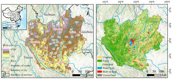
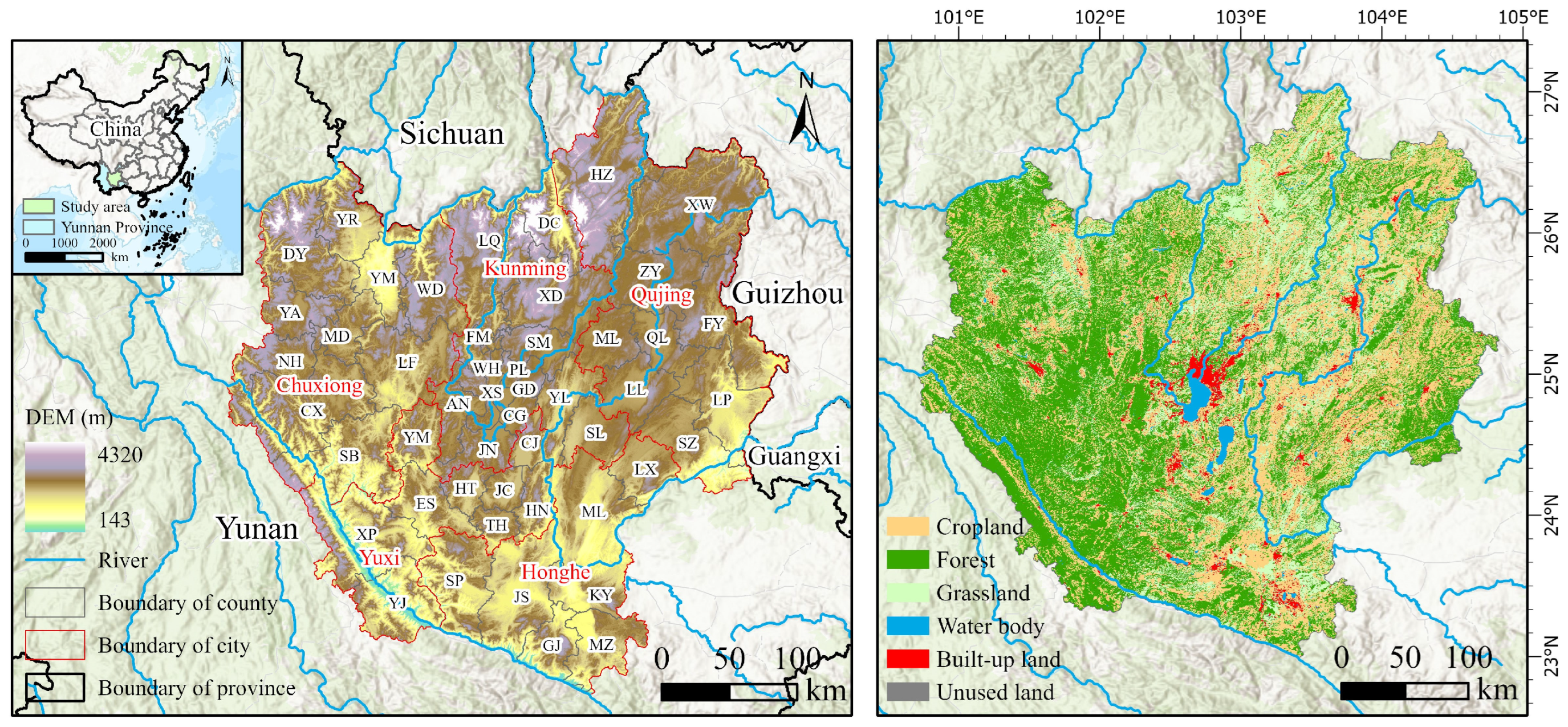
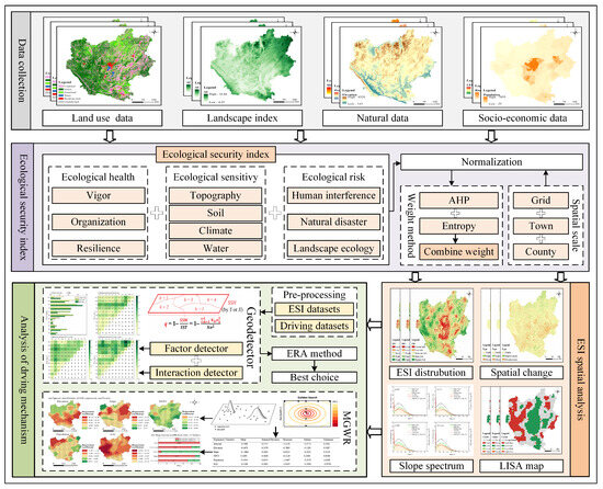
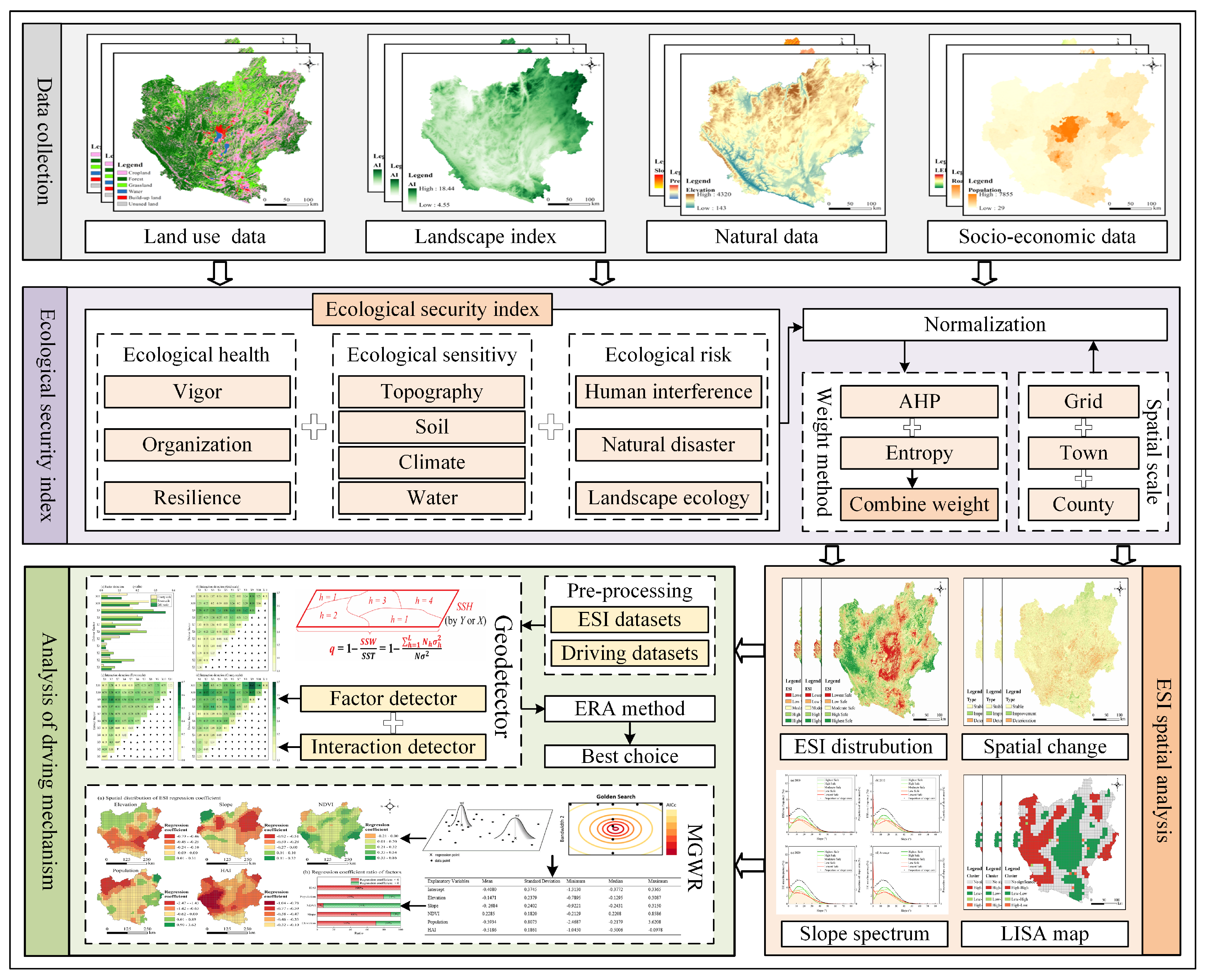
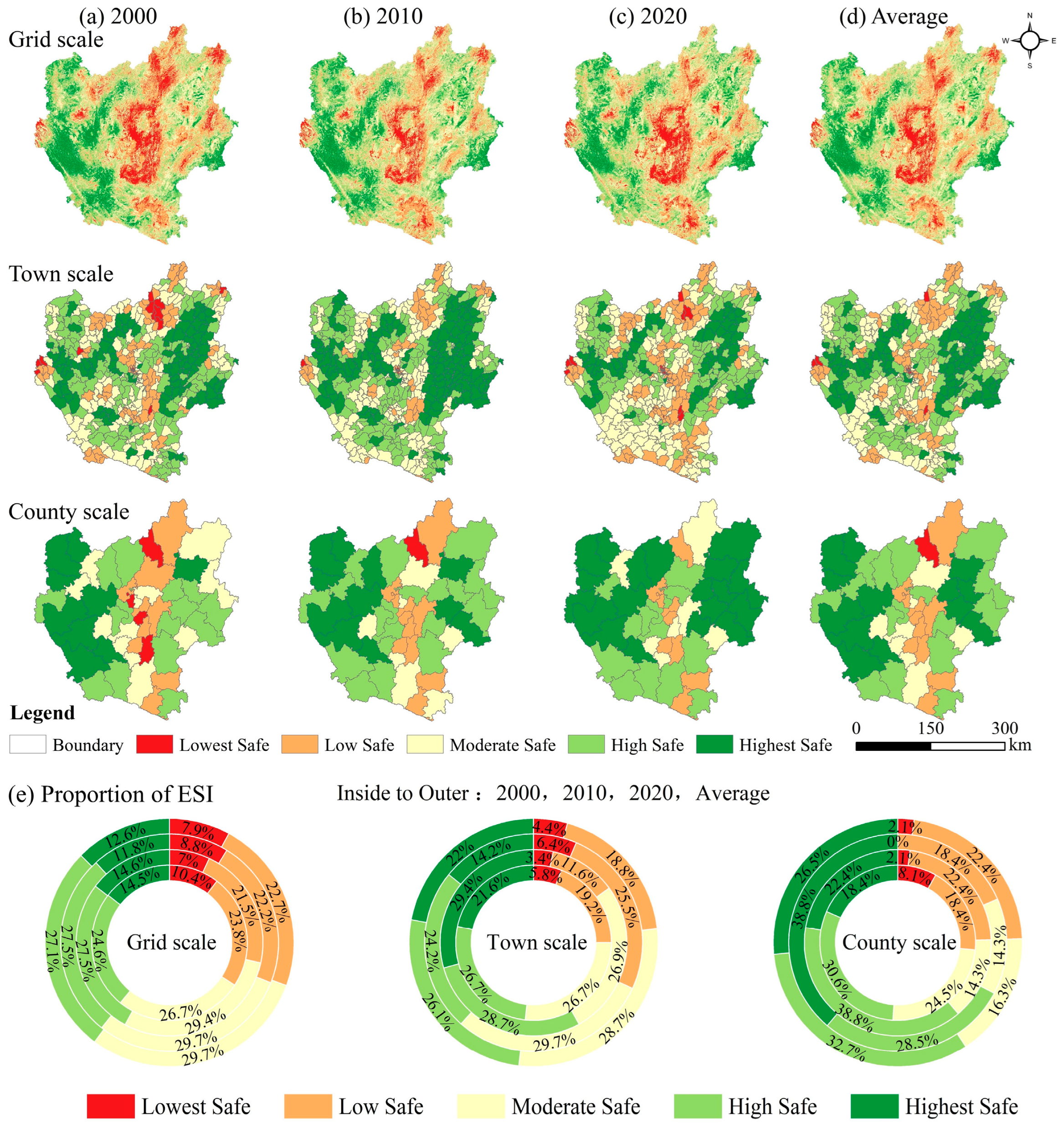
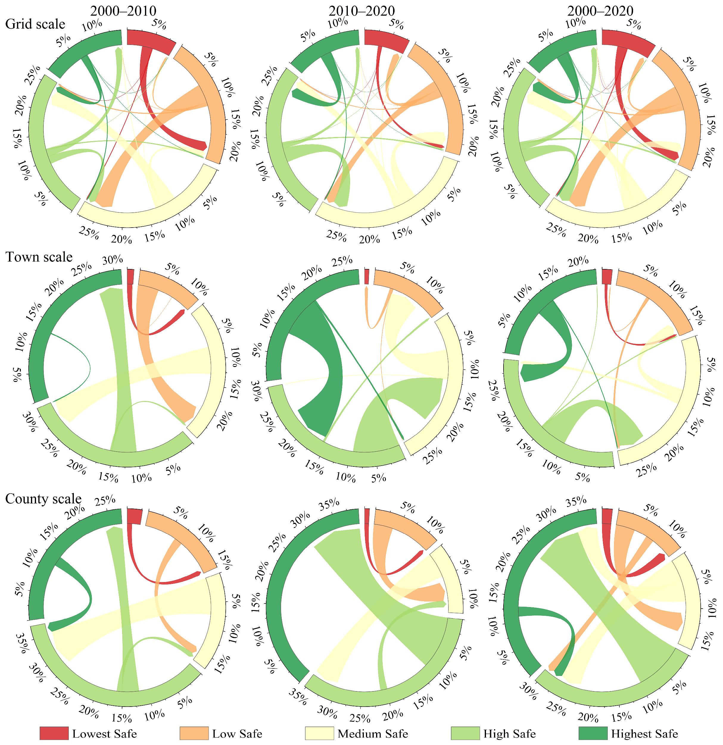
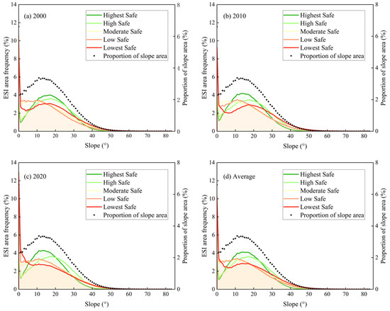
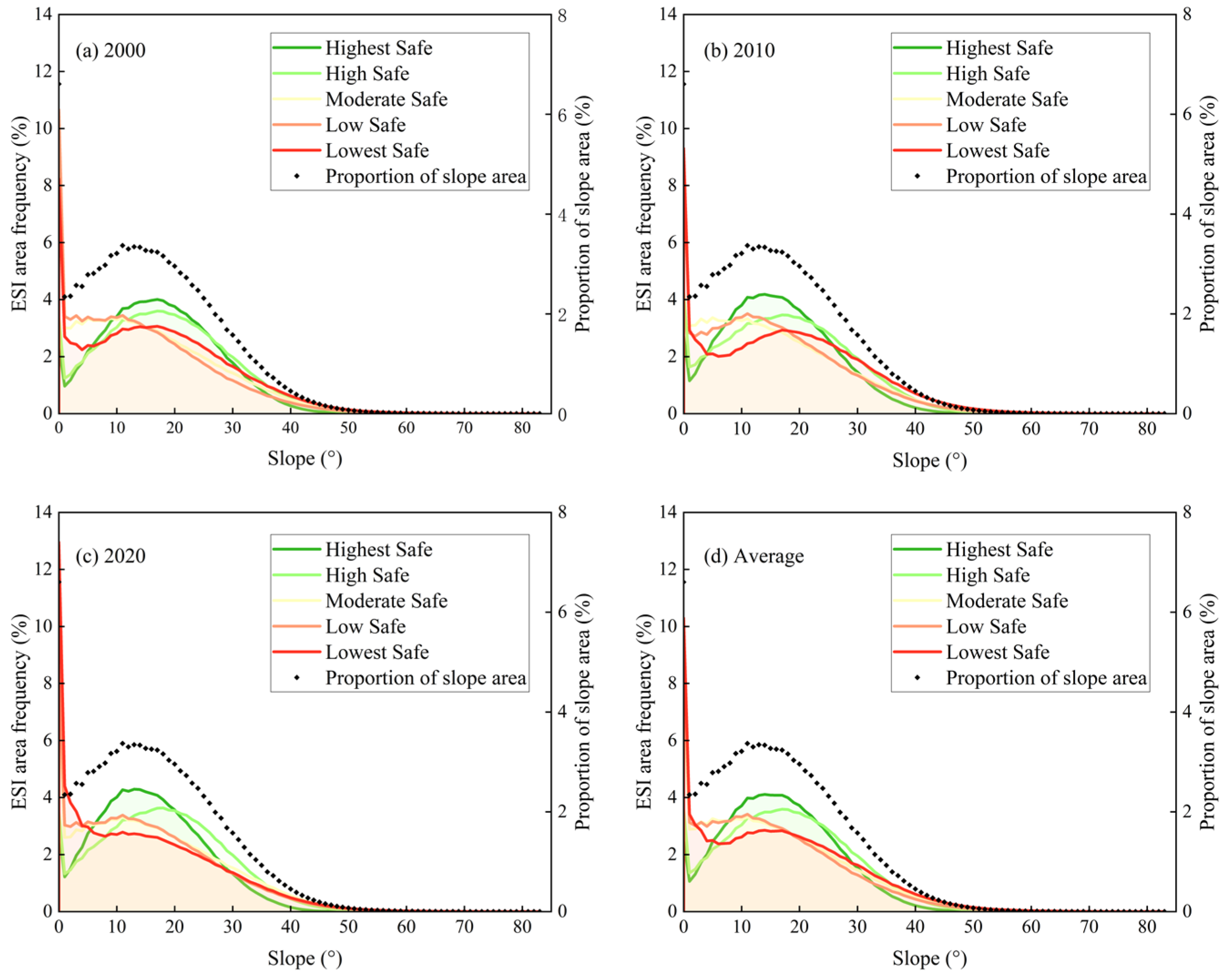
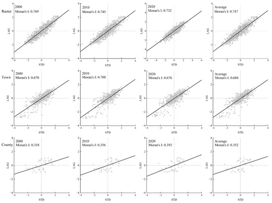
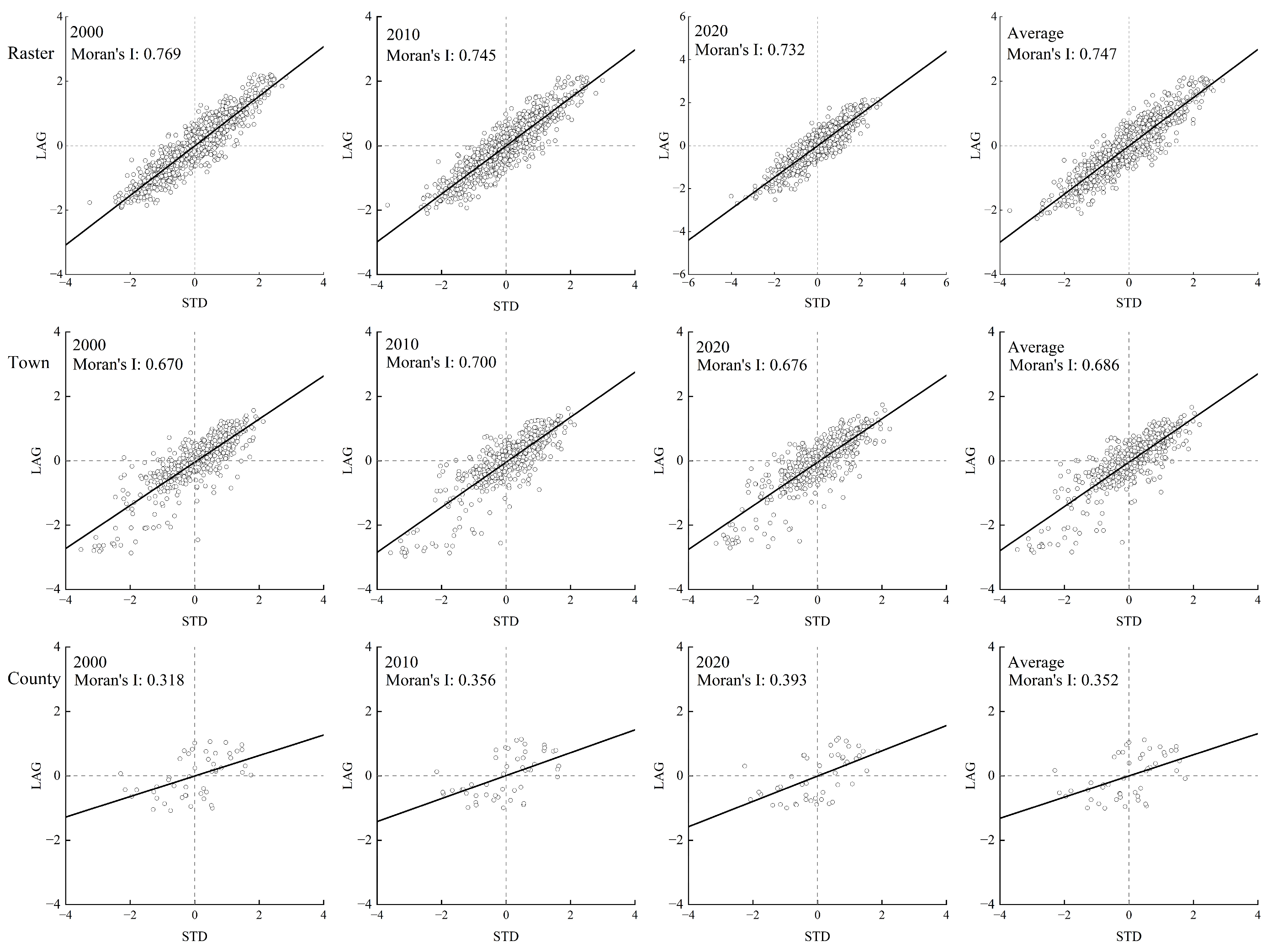
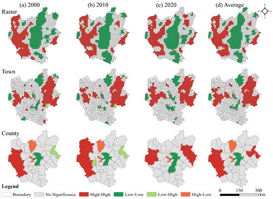
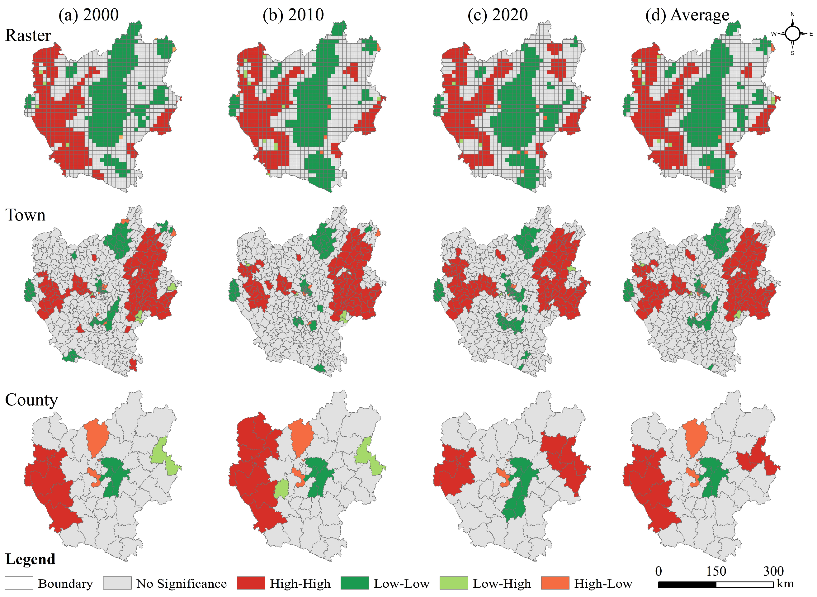
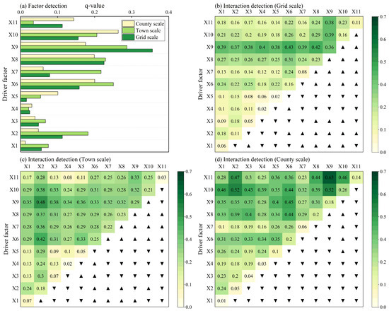
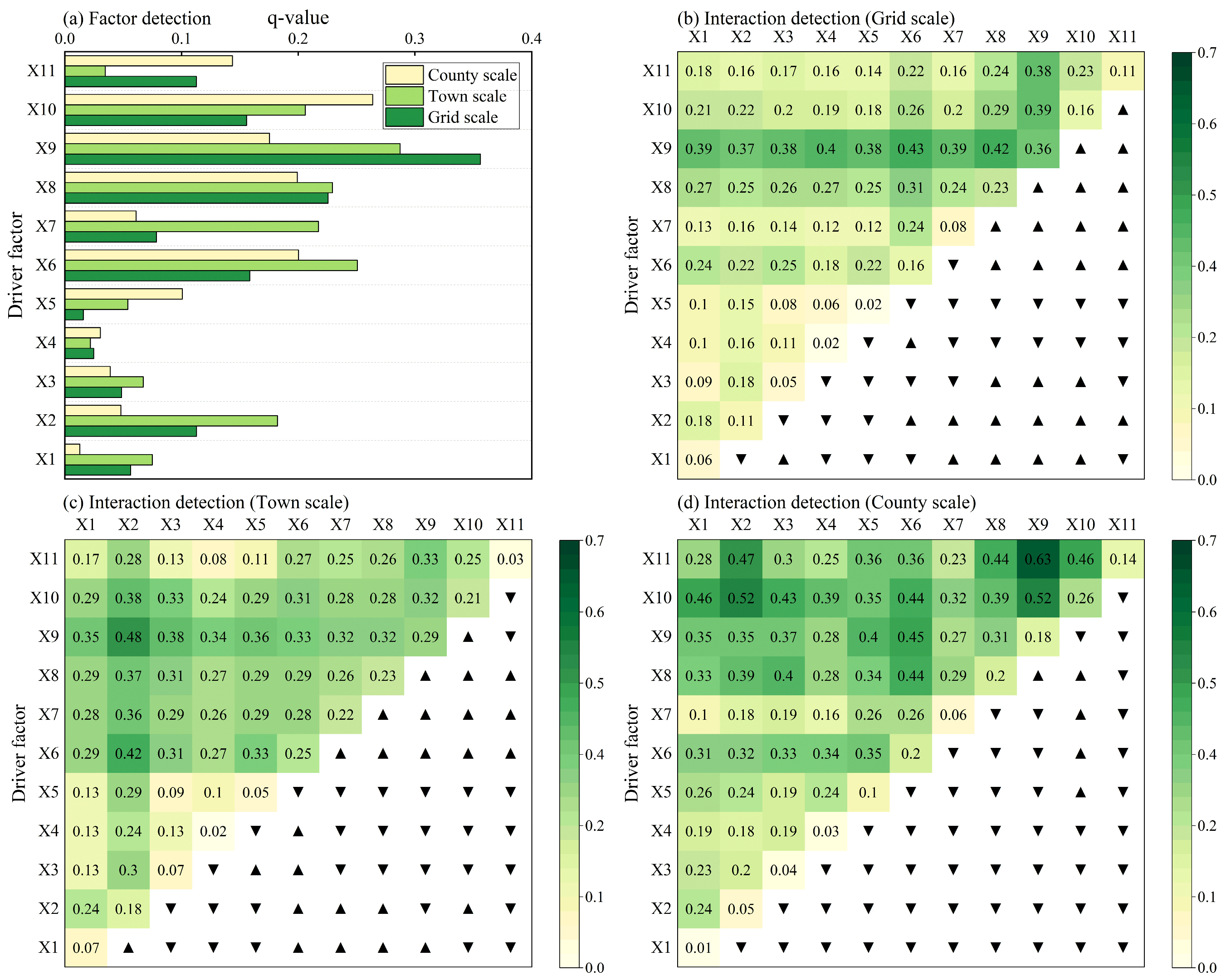
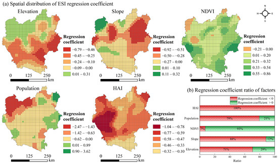
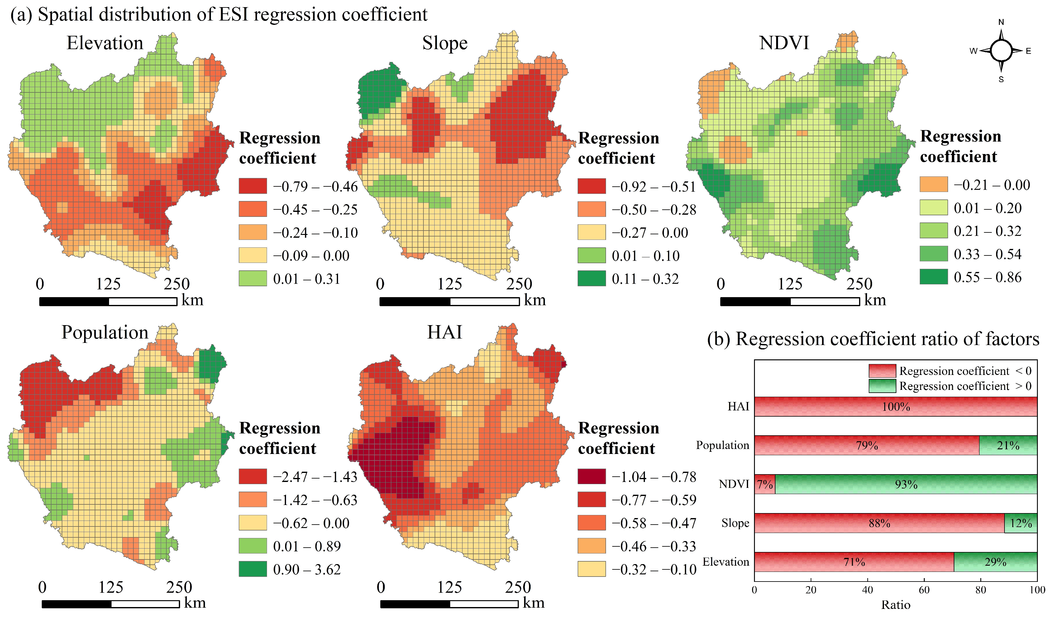
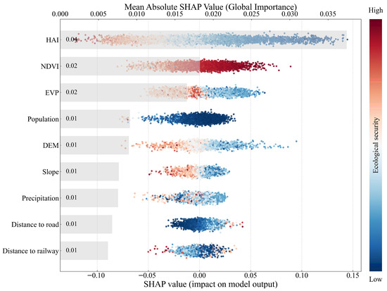
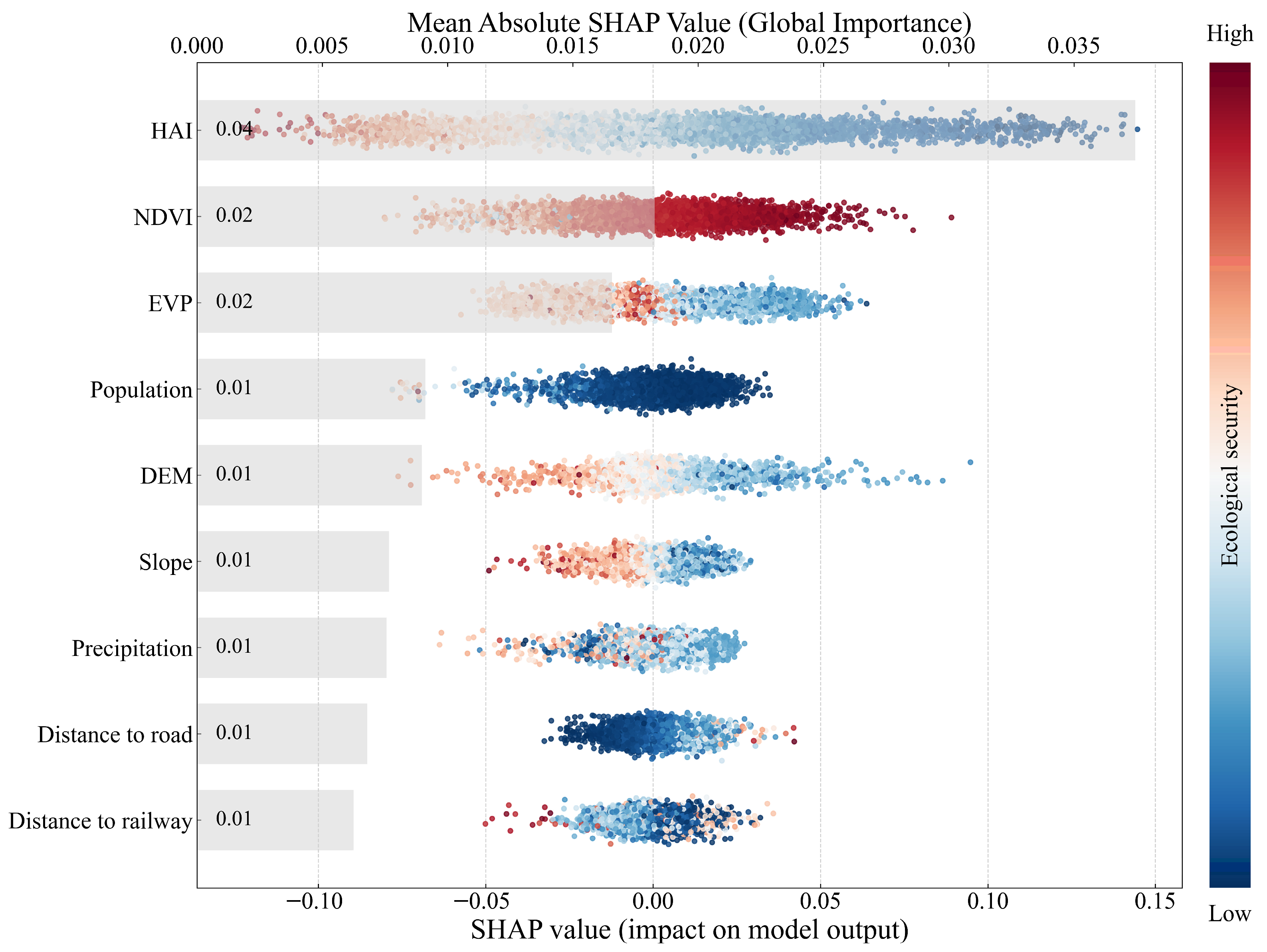
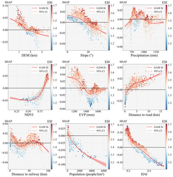
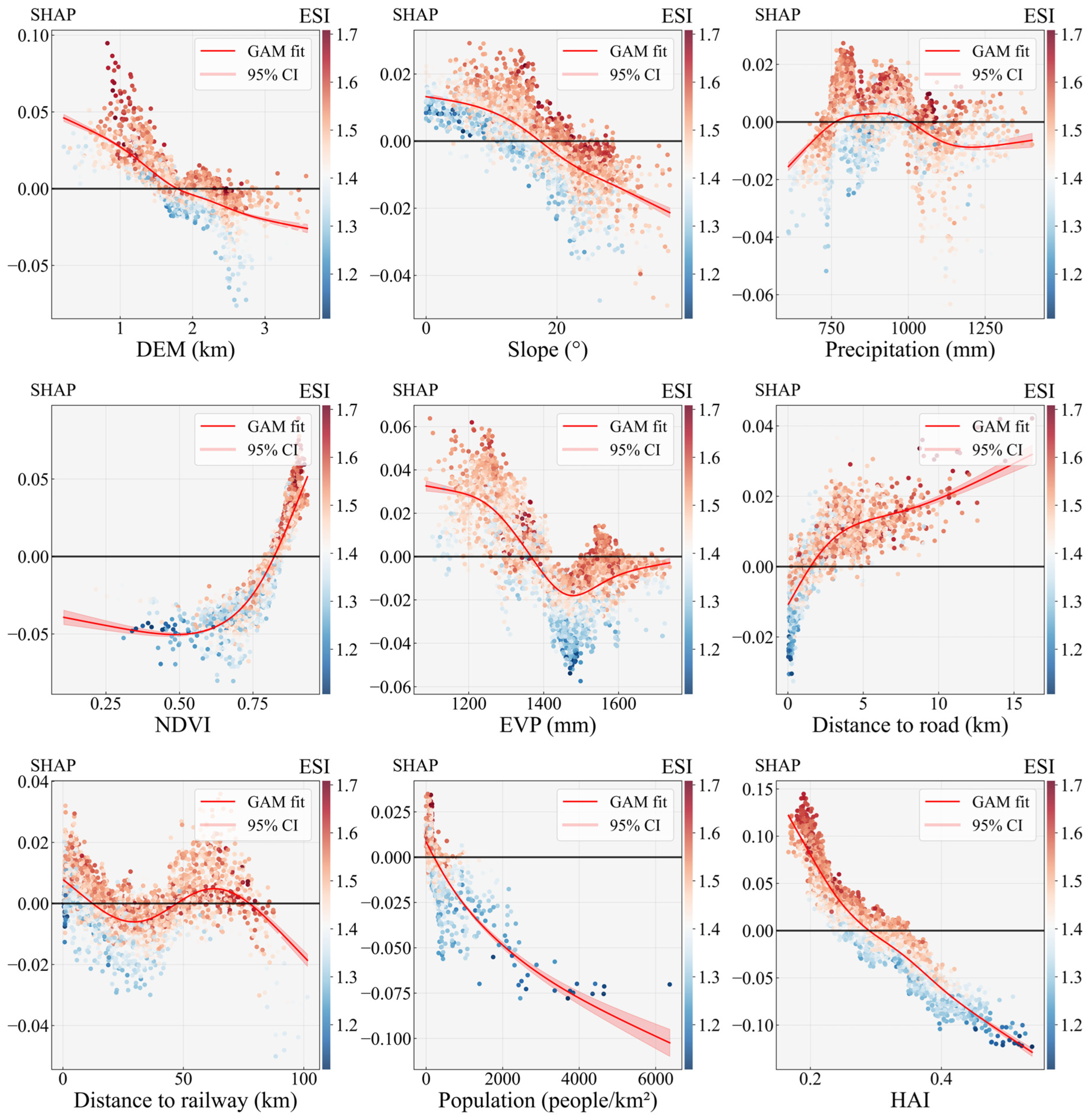

Disclaimer/Publisher’s Note: The statements, opinions and data contained in all publications are solely those of the individual author(s) and contributor(s) and not of MDPI and/or the editor(s). MDPI and/or the editor(s) disclaim responsibility for any injury to people or property resulting from any ideas, methods, instructions or products referred to in the content. |
© 2026 by the authors. Licensee MDPI, Basel, Switzerland. This article is an open access article distributed under the terms and conditions of the Creative Commons Attribution (CC BY) license.