


Abstract
Land use/land cover (LULC) exerts a substantial influence on hydrological processes, notably runoff generation, flow routing, and evapotranspiration. To evaluate the impacts of LULC change on different flood types in the Jinhua River Basin, LULC data from four periods (2005, 2015, 2025, and 2035) were incorporated into the Distributed Hydrology–Soil–Vegetation Model (DHSVM). Using a fuzzy decision tree approach, thirty-six flood events were identified and classified as flash floods (FFs), short-rainfall floods (SRFs), and long-rainfall floods (LRFs). Projections of LULC for 2035 under three Shared Socioeconomic Pathways (SSP1-2.6, SSP2-4.5, and SSP5-8.5) were generated by coupling System Dynamics (SD) with the Patch-based Land Use Simulation (PLUS) model. DHSVM was calibrated separately for each flood category, with the 2005 LULC dataset serving as the baseline for parameter estimation. The results revealed a progressive decline in forest land and water from 2005 to 2035, together with an expansion of construction land. By contrast, cultivated land exhibited a fluctuating pattern, expanding initially, then contracting, and recovering thereafter. These land-cover changes increased flood volumes and peak flows across FF, SRF, and LRF alike, largely owing to the growth of construction land and the loss of forest cover and water. Across the three future scenarios, the largest increases were projected under SSP5-8.5, followed by SSP2-4.5 and SSP1-2.6. With respect to flood type, LULC change exerted the most pronounced effects on flood volume and peak flow for LRF, followed by SRF and FF. Under SSP5-8.5, the maximum relative changes in LRF reached 6.74% in flood volume and 8.56% in peak flow. These findings suggest that LRF warrant greater attention in future assessments given their comparatively higher potential risk. Such divergent responses of the three flood types to LULC change can be attributed primarily to intrinsic differences in their flood characteristics.
1. Introduction
Substantial LULC changes have occurred under the combined influence of climate change and intensive human activities, with urban areas particularly affected [1,2]. It is widely acknowledged that LULC change substantially alters water resources and hydrological processes [3,4]. Key hydrological components, including surface runoff, base flow, canopy interception of precipitation, and evapotranspiration, can be modified by such change within a catchment. Consequently, the rainfall runoff conversion pathway is reshaped, ultimately affecting regional water availability [5,6,7].
Numerous studies have demonstrated that LULC change plays a pivotal role in regulating water resources and hydrological processes. For instance, Zhan et al. [8] reported that grassland changes in the source region of the Yellow River enhanced evapotranspiration and soil moisture storage by 5.66% and 2.03%, respectively. Markhali et al. [9] examined the hydrological responses to pronounced LULC change across 89 catchments in Eastern North America and found that spring peak flows associated with snowmelt shifted markedly in both magnitude and timing. Naha et al. [10] integrated Land-Use Harmonization version 2 (LUH2) data into the Variable Infiltration Capacity (VIC) model to assess the effects of LULC change on hydrological responses in a large Indian river basin; their results revealed a median percentage increase in extreme flows, while mean annual flows rose by 1.8–11.3% across the subcatchments. Liu et al. [11] further showed that the expansion of cropland, grassland, and urban areas increased river runoff, whereas the growth of forest area reduced it.
Taken together, the above literature indicates that LULC change exerts a pronounced influence on hydrological processes, with its effects on flood events being of particular concern given the direct implications for flood mitigation and risk assessment. Avashia and Amit [12] examined the role of LULC change in the occurrence of urban flooding across 42 Indian cities under both historical and future scenarios. Their findings indicated that flood frequency rose with urban expansion, and that the number of flood events under Representative Concentration Pathway (RCP) 2.6 was considerably lower than under RCPs 4.5 and 8.5. Gao et al. [13] identified forest as the land use type most sensitive to flood retention, with increased forest cover contributing to reduced flood magnitudes. However, the expansion of forest area did not lower the frequency of 5-year and 10-year return period floods. Liu et al. [14] demonstrated that human activities, particularly deforestation and polder expansion, exerted a more pronounced effect on millennial flood regimes in the Yangtze River Basin than meteorological factors did. Collectively, these studies have primarily addressed aggregated flood events, while limited attention has been given to the distinct mechanisms through which LULC change affects different flood types [12,13].
Therefore, this study aims to explore how historical and future LULC changes affect different flood types, specifically with respect to flood volume, peak flow, and time to peak. To this end, DHSVM, a physically based and fully distributed hydrological model, is employed to simulate flood events of various types under LULC conditions from different periods and subsequently assess the resulting changes in these events [15]. Compared with other hydrological models, DHSVM is better suited to catchments with small drainage areas [16]. Because it incorporates approximately twenty parameters for each land use type, such as leaf area index (LAI), vegetation albedo, and vegetation resistance, the model can adequately represent the distinct characteristics of each land use type, thereby capturing the influence of LULC change on flood events [17]. Its spatial resolution is determined by that of the digital elevation model (DEM), typically 30 m, and its temporal resolution ranges from hourly to daily [17]. Consequently, DHSVM can produce simulation outputs with high spatial and temporal resolution. In a study by Zhan et al. [8], DHSVM was applied to evaluate the influence of grassland surface area and growth state on hydrological processes in the source region of the Yellow River, with growth state quantified using LAI. Similarly, Zhang et al. [18] used DHSVM to investigate historical and future runoff responses in the Kaidu River Basin across various scenarios of climate and LULC change.
Future LULC data for 2035 are also projected under multiple scenarios using the SD-PLUS model, which has been widely adopted for this purpose owing to its ease of use and reliable accuracy. For instance, Zhao et al. [19] applied this approach to simulate LULC patterns in Jilin Province for 2030 across four development scenarios, and Yuan et al. [20] projected LULC in Wuhan for 2030 under SSP1-2.6, SSP2-4.5, and SSP5-8.5. These scenarios are generally considered appropriate and feasible for LULC-related studies. Although the SSP-RCP framework theoretically encompasses 30 combinations (5 SSPs × 6 RCPs), applying all of them is impractical owing to computational limitations [21]. Consequently, three representative scenarios are commonly selected for further analysis: a low-emission scenario (SSP1-RCP2.6), a moderate-emission scenario (SSP2-RCP4.5), and a high-emission scenario (SSP5-RCP8.5) [22,23]. These three scenarios are therefore adopted in the present study.
This study focuses on the Jinhua River Basin, located in East China. Owing to the uneven distribution of precipitation, the basin frequently experiences flooding during the typhoon and plum rain seasons. Understanding how LULC change influences flood hazards is therefore essential, as such knowledge can support more effective flood risk management and disaster prevention. Accordingly, this study pursues three main objectives: (1) to analyze LULC change during the historical period from 2005 to 2025; (2) to project future LULC patterns for 2035 under the SSP1-2.6, SSP2-4.5, and SSP5-8.5 scenarios and examine LULC changes from 2025 to 2035; and (3) to evaluate the impacts of historical and future LULC changes on multiple flood types using the DHSVM model.
2. Materials and Methods
Figure 1 illustrates the overall flowchart of this study, which comprises three main modules: projecting future (2035) LULC demand using the SD model, simulating future spatial LULC patterns with the PLUS model, and assessing the influence of historical and future LULC change on different flood types using the DHSVM model. For the SD model, driving data (Section 2.1.2) and historical LULC data are employed to determine LULC demand in the Jinhua River Basin. Once the model attains acceptable accuracy, it is applied to project LULC demand for 2035 under three scenarios (SSP1-2.6, SSP2-4.5, and SSP5-8.5). For the PLUS model, historical LULC data and driving factors are adopted to construct the LULC simulation model. Following validation of its accuracy, the PLUS model is used to project the spatial distribution of LULC in 2035 under the same scenarios, with the demand constrained by the SD model outputs. Subsequently, flood events are identified from the observed runoff series using the automated selection procedure, and the fuzzy decision tree method is applied to classify these events into three flood types: FF, SRF, and LRF. Hydro-meteorological and geographical data are then used to configure DHSVM separately for each flood type, followed by parameter calibration using the 2005 LULC data. Once the model exhibits acceptable performance for all three flood types during both calibration and validation, the LULC maps for 2015, 2025, and 2035 (under the three scenarios) are fed into the calibrated model to generate the corresponding simulations. Notably, only the vegetation map is replaced with the LULC maps for 2015, 2025, and 2035, while all other model inputs remain unchanged. Finally, the simulated changes are systematically evaluated in two parts: the first examines the impacts of historical LULC change (2005 and 2025) on the different flood types, and the second examines those of future LULC change (2035) under the three scenarios.
Figure 1.
The flowchart of this study.
2.1. Study Area and Data
2.1.1. Study Area
The Jinhua River Basin is a major tributary of the Qiantang River Basin, which is the longest and largest river system in Zhejiang Province, East China. As illustrated in Figure 2, the Jinhua River Basin is situated in the mid-western part of Zhejiang Province and covers a drainage area of 5897 km2 above the Jinhua discharge station, the basin outlet [24]. Geographically, the basin extends from 28.5° N to 29.5° N in latitude and from 119.4° E to 120.7° E in longitude, with elevations ranging from 29 m to 1284 m. The study area is predominantly influenced by an Asian subtropical monsoon climate, characterized by abundant precipitation and high temperatures in summer and by cold and dry conditions in winter. The mean annual precipitation is approximately 1400 mm [25]. Owing to the unevenly distributed precipitation, the catchments are highly susceptible to flood disasters, posing significant risks to residents and property. Accurate flood simulation is therefore essential, as it provides critical support for flood prevention. Moreover, LULC change exerts a considerable influence on flood characteristics. As shown in Figure 2, the land use types within the study area comprise forest land, water, cultivated land, and construction land. In 2005, forest land and cultivated land were the dominant land use types, accounting for 64.01% and 27.33% of the total area, respectively, whereas water and construction land represented 1.5% and 7.17%.
Figure 2.
The location, DEM, streams, meteorological stations, discharge station and LULC (2005) of the study area. (a) Location of study area; (b) DEM of study area; (c) LULC (2005) of study area.
2.1.2. Data
- LULC dataset
This study employs the China Annual Land Cover Dataset (CLCD), which was developed by Wuhan University from Landsat imagery and spans the period from 1985 to 2025 [26]. Its spatial resolution is 30 m. A post-processing method based on spatiotemporal filtering was incorporated into the dataset, and logical reasoning was introduced to improve the spatiotemporal consistency of the CLCD. Owing to its accessibility, accuracy, adequate temporal coverage, and high spatial resolution, the CLCD has been widely adopted. For this study, a total of 19 years of data (2005 and 2008–2025) were used. The dataset is publicly available at https://zenodo.org/records/15853565 (accessed on 1 July 2026).
- Input data for SD model
A total of eleven input variables were used in the SD model: gross domestic product (GDP), total population, rural population, urban population, precipitation, temperature, urbanization rate, fixed asset investment, fishery output value, agricultural output value, and forestry output value. These variables, comprising both socioeconomic and climatic data, were obtained from the Jinhua Statistical Yearbook (http://tjj.jinhua.gov.cn/col/col1229166308/index.html, accessed on 8 July 2026), which covers the period from 2008 to 2024. All inputs to the SD model are annual values.
- Driving factors datasets for PLUS model
The driving factors for the PLUS model fall into four categories: climatic, physical geographical, socioeconomic, and locational factors. As shown in Table 1, the climatic data include precipitation and temperature for 2025, both at a spatial resolution of 1 km, which were downloaded from the Resource and Environmental Science Data Platform of the Chinese Academy of Sciences (RESDC) (https://www.resdc.cn). The physical geographical factors consist of DEM, slope, soil data, and the normalized difference vegetation index (NDVI) for 2025. The DEM has a spatial resolution of 30 m and was sourced from https://www.gscloud.cn/, whereas the slope, soil, and NDVI datasets have resolutions of 500 m, 1 km, and 1 km, respectively, and were obtained from RESDC. The socioeconomic factors comprise GDP and population data for 2023, both at a resolution of 1 km [27]. For the locational factors, road information was obtained from RESDC, and stream networks were generated from the DEM. Distance variables were derived through Euclidean distance analysis. The data used in the PLUS model are maps matched to the LULC. The spatial distributions of these driving factors within the Jinhua River Basin are presented in Figure 3.
Table 1.
Driving factors used for PLUS model.
Figure 3.
Driving factors used for PLUS model. (a) DEM; (b) Slope; (c) Soil; (d) NDVI; (e) Temperature; (f) Precipitation; (g) GDP; (h) Population; (i) Distance to expressway; (j) Distance to railway; (k) Distance to national highway; (l) Distance to provincial highway; (m) Distance to streams.
- Data for DHSVM model
The DHSVM model requires both geographical and hydro-meteorological data. The meteorological variables include precipitation, average air temperature, wind speed, relative humidity, and incoming longwave and shortwave radiation. A total of 23 meteorological stations were used in this study, and their locations are shown in Figure 2. Most of these stations provide complete records of the aforementioned variables for the period from 1 January 2006 to 31 August 2014 (see Table 2). Missing data at several stations were filled by inverse distance interpolation using data from the nearest stations. The hydrological data consist of observed runoff at the Jinhua discharge station, covering the period from 4 December 2006 to 1 July 2013. Both datasets are available at an hourly temporal resolution.
Table 2.
The meteorological stations used in this study.
The geographical data required for the DHSVM model comprise the basin boundary (mask), DEM, soil data, LULC data, soil depth, and stream network. The DEM was obtained from https://www.gscloud.cn/ at a spatial resolution of 30 m, and the basin mask was derived from the DEM. Soil data were acquired from the Nanjing Institute of Soil Research and subsequently reclassified according to the U.S. Department of Agriculture (USDA) soil texture classification system, as required by the DHSVM model. LULC data were extracted from the CLCD dataset for 2005, while the stream network and soil depth were generated from the DEM and basin mask. Given that model calibration at the native 30 m resolution would take several months and impose a considerable computational burden, all geographical datasets were resampled to a 200 m spatial resolution by nearest-neighbor resampling. At this resolution, model calibration requires several days on a small server (24 cores, 48 threads). Accordingly, all subsequent model runs were performed at the 200 m resolution to balance computational efficiency and simulation accuracy.
2.2. Methods
2.2.1. Multi-Scenario Setting
This study adopts SSP-RCP scenario combinations to project future LULC in the Jinhua River Basin. The SSP-RCP framework, which is widely applied in the Coupled Model Intercomparison Project Phase 6 (CMIP6) and related research, couples the Shared Socioeconomic Pathways (SSPs) with the Representative Concentration Pathways (RCPs). Three commonly used scenarios were selected: SSP1-2.6, SSP2-4.5, and SSP5-8.5. These scenarios were subsequently applied to generate the 2035 LULC map for the basin. Specifically, SSP1-2.6 (SSP1-RCP2.6) represents a low-emission pathway that combines strong climate mitigation with sustainable development. SSP2-4.5 (SSP2-RCP4.5) corresponds to a moderate-emission pathway with intermediate mitigation efforts, consistent with the continuation of current socioeconomic and technological trends. SSP5-8.5 (SSP5-RCP8.5) describes a high-emission pathway characterized by energy-intensive socioeconomic development and elevated radiative forcing. The detailed parameter settings for the three scenarios are provided in Table 3. GDP and population growth rates were established according to the development targets outlined in the Jinhua 14th Five-Year Plan, whereas other parameters, such as the annual average temperature and precipitation variations, were determined based on previous studies [28,29].
Table 3.
Scenario parameter settings for 2035.
2.2.2. SD-PLUS Model
- SD model
The SD model is employed to elucidate the dynamic interactions among demographic, economic, and climatic drivers, thereby evaluating their combined influence on LULC change [30]. The version used in this study is Vensim PLE 7.3.5. The model subsequently forecasts LULC transitions and the corresponding demand areas for each land use type in the Jinhua River Basin (Figure 4; the SD model equations are shown in Table S1). On the basis of previous studies, five interconnected subsystems (LULC, productivity, economy, climate, and population) are established to construct the LULC demand system. A total of eleven variables are included, as detailed in Section 2.1.2. The simulation period spans 2008 to 2035, with 2008–2024 serving as the historical calibration period and 2025–2035 used to project future LULC demand. A one-year time step is adopted. The calibration period extends only to 2024 because statistical data for 2025 are not yet publicly available. The evaluation index for accuracy estimation in the SD model is the relative error (RE) [31], and its equation is given as follows:
Figure 4.
The reproducible stock-flow structure of the SD model.
- PLUS model
The PLUS model comprises two primary modules: the land expansion analysis strategy (LEAS) and a cellular automaton (CA) model that employs multiple random seeds (CARS) [32]. The version used in this study is PLUS v1.40. The LEAS module performs a comparative analysis of LULC data between 2005 and 2015 to identify transition patterns among changing land use types by examining their expansion patches. A random forest classification algorithm is then applied to estimate the development probability of each land use type on the basis of the influence of multiple driving factors on land use growth [31]. These driving factors and their data sources are described in Section 2.1.2. Both the LULC maps and the driving factors have a spatial resolution of 30 m. The CARS module, built upon a cellular automaton framework, functions as a scenario-driven simulation model that reproduces the spatial distribution of LULC using the development probabilities generated by the LEAS module [33]. In this study, the development probabilities derived for the period 2005–2015 were used in the CARS module to simulate the LULC distribution in 2025. The simulated results were subsequently validated against the observed LULC distribution in 2025 using the Kappa coefficient, overall accuracy (OA), and the figure of merit (FoM). The corresponding equations are presented as follows:
2.2.3. Flood Event Selection and Flood Type Classification
- Flood event selection
This study applies an automated procedure to identify flood events from the observed runoff series [35]. The procedure comprises three main steps: (1) detecting the peak flow in the hourly observed runoff series; (2) identifying the start and end times of each flood event, defined as the moments when runoff falls below a specified threshold; and (3) if precipitation is present at the initially identified start time, adjusting the start time backward to the most recent moment with no precipitation. Further details of this method are provided in our previous study [24]. A total of 36 flood events are identified for subsequent analysis.
- flood type classification
A process-based flood classification method is employed in this study [36]. This approach categorizes floods into five types: flash floods (FFs), short-rain floods (SRFs), long-rain floods (LRFs), rain-on-snow floods, and snowmelt floods. Given the limited snowfall in the Jinhua River Basin, only rainfall-related flood types are considered. FFs typically occur during the typhoon season and result from short-duration, high-intensity precipitation. Such events are usually localized. SRFs can occur throughout the year and are generated by rainfall of relatively short duration and high intensity; they differ from FFs in their larger spatial extent and longer duration. LRFs also occur year-round and are driven by prolonged, low-intensity precipitation ranging from several days to weeks. This flood type is generally regional in scope and may affect the entire river basin [36].
Subsequently, the fuzzy decision tree approach (the structure shown in Figure S1) is applied to classify the 36 selected events into multiple flood types. Within this framework, an individual event may comprise more than one flood type. The method yields a degree of acceptance for each event across all categories, and the type with the highest acceptance is designated as the primary flood type [37]. The fuzzy decision tree method is described in further detail in our previous study [24]. The classification is based on precipitation duration and intensity, event timing, and other factors (Table 4). On this basis, the 36 flood events are assigned to three categories: 18 to SRF, 13 to LRF, and 5 to FF. The median flood durations of the three types are 142 h for LRFs, 84 for SRFs, and 57 for FFs [24].
Table 4.
Flood indicators used for fuzzy decision tree classification.
2.2.4. DHSVM Model Set-Up and Calibration
DHSVM is a fully distributed and physically based hydrological model capable of simulating hydrology and vegetation dynamics [15,16]. The version used in this study is DHSVM 3.1.1. The model discretizes the catchment into computational grids based on the DEM, and for each grid cell it solves the water and energy balance equations simultaneously. For each grid cell, the vegetation and soil types are assigned from the input vegetation and soil maps. Each soil type is described by 17 parameters, such as lateral conductivity, field capacity, and wilting point. Each land use type is described by approximately 20 parameters, including leaf area index, vegetation albedo, and vegetation resistance. For cells classified as impervious construction land, the impervious surface fraction is also specified. Precipitation falling on impervious surfaces becomes surface runoff, and the proportion of this runoff routed directly to streams varies with land cover. Open water is treated as a distinct vegetation type, primarily characterized by an impervious fraction of 1.0, so that all precipitation becomes surface runoff that is routed directly to stream channels. The simulated physical processes include snowpack accumulation and melt, canopy snow interception and release, evapotranspiration, unsaturated moisture movement, saturated subsurface flow, surface flow, and channel flow [17]. DHSVM has been widely and successfully applied in studies of climate change, stream temperature modeling, and urbanization [25,38]. The model can operate at daily or sub-daily time steps. In this study, an hourly temporal resolution and a 200 m spatial resolution were adopted.
The input data for the DHSVM model are described in Section 2.1.2. Parameter identification was performed with the ε-dominance non-dominated sorting genetic algorithm II (ε-NSGA-II) [39,40], a many-objective evolutionary algorithm. Unlike Bayesian inference schemes such as MCMC, which sample a posterior distribution p(θ | D) over the parameter space, ε-NSGA-II searches for an ε-approximation of the Pareto-optimal set, i.e., the set of parameter vectors that are mutually non-dominated with respect to the four calibration objectives (KGE, PBIAS, PPBIAS, and ΔT). A multi-objective formulation was adopted because these objectives are in competition, so that no single parameter vector can optimize all of them simultaneously. The algorithm was run with an objective-wise ε and a fixed upper limit on the number of archived solutions, and it was terminated once the ε-progress indicator showed no further improvement over consecutive generations. Because the ε-dominance archiving strategy guarantees a bounded archive size and monotone improvement of the ε-indicator irrespective of the number of objectives [41], convergence to a representative approximation of the Pareto set is a designed property of the algorithm rather than a post hoc empirical check. The archived set analyzed here is therefore a converged ε-nondominated archive rather than the final generation of a single trajectory.
Calibration was performed separately for each of the three flood types. Following the commonly used 7:3 calibration-to-validation ratio in hydrological modeling, the available flood events were allocated to calibration and validation as closely as possible to this ratio. For FFs, 3 flood events were used for calibration and 2 for validation; for SRFs, 12 events were used for calibration and 6 for validation; and for LRFs, 9 and 4 events were used for calibration and validation, respectively. The parameters selected for calibration were determined based on the sensitivity analysis results of our previous study [24], in which a local sensitivity test was conducted using a one-at-a-time parameter perturbation approach, a method well validated in previous DHSVM applications. Based on the sensitivity results, 12 sensitive parameters (Table 5) were selected for calibration. By calibrating with ε-NSGA-II, a set of Pareto-optimal solutions was obtained. Each Pareto-optimal solution represents a feasible parameter configuration that is not dominated by any other across all objective functions. Because no single best solution exists on the Pareto front, a compromise solution was selected for each calibration scenario. This solution was identified by minimizing the normalized Euclidean distance from each Pareto-optimal solution to the ideal point, which is defined by the optimal value of each objective function, as described in the following paragraph.
Table 5.
Twelve sensitive parameters used for model calibration.
The objective functions used for model calibration comprise the Kling-Gupta Efficiency (KGE) [42,43], absolute percent bias for flood volume (PBIAS) and peak flow (PPBIAS), and the ratio of peak time error to flood duration (ΔT). The optimal value of KGE is 1, whereas the optimal values of PBIAS, PPBIAS, and ΔT are all 0. The acceptance criterion for KGE is >0.5 [44]. The acceptance criteria for PBIAS and PPBIAS are ≤30% and ≤20%, respectively [45,46]. For ΔT, no explicit criterion has been established; however, lower values are generally preferable [47]. The four evaluation indices are defined as follows:
where α represents the proportion of the standard deviation of simulated runoff to the standard deviation of observed runoff; β is the proportion of simulated mean runoff to observed mean runoff; indicates the correlation coefficient between simulated runoff and observed runoff series for a certain flood event. Si and Oi are simulated and observed runoff at time step i; i1 and i2 are the beginning and end time for a certain flood event; Sp and Qp are simulated peak flow and observed peak flow; t(Sp) and t(Qp) are simulated and observed peak flow occurrence times; T denotes the flood duration for a certain flood event. The aforementioned evaluation indices are first calculated for each flood event individually. The final value for each flood type is then obtained by averaging the results across all events within that type.
3. Results
3.1. Accuracy Evaluation of SD-PLUS Model
3.1.1. SD Model
Figure 5 compares the simulated and observed areas of all land use types in the Jinhua River Basin for 2024. The differences between the simulated and observed values for cultivated land, forest land, water, and construction land in 2024 are −1.89 km2, −23.95 km2, 1.96 km2, and 13.18 km2, respectively. The corresponding RE values are −0.12%, −0.68%, 2.76%, and 1.79%. All RE values fall within ±3%, below the acceptable threshold of ±5% (see Table 6). Moreover, the RE values for all land use types during 2008–2023 remain within ±5%, indicating that the model accuracy meets the required standard. These results confirm that the developed SD model is suitable for projecting LULC demand in 2035 under multiple scenarios. For all four land use types, the residuals are free of significant linear dependence on the predicted values (R2 between Re and Pr = 0.00–0.20; all p > 0.05) and of scale-dependent bias (Figure S2). The DW statistic of 0.37, 1.19, 0.51, and 0.41 computed on the level residuals is not diagnostic, because the residuals of two smooth, strongly trending series are serially correlated by construction; computed on the first-differenced residuals, which removes the trend, it becomes 2.00, 2.51, 1.44, and 2.01, all within the no-autocorrelation region [dU, 4 − dU] = [1.37, 2.63], indicating no systematic short-term temporal structure.
Figure 5.
Comparison of the simulated area and actual area in 2024.
Table 6.
RE (%) values of each land use type during 2008–2024.
3.1.2. PLUS Model
In the PLUS model, the LULC distributions for 2005 and 2015 are first used to derive the development probability of each land use type; these probabilities are then employed to simulate the LULC distribution in 2025. Figure 6 compares the actual (a) and simulated (b) LULC distributions in 2025. The simulated spatial distribution closely matches the actual distribution. For the 2025 simulation, the Kappa coefficient is 0.85, the FoM index is 0.14, and the overall accuracy reaches 0.92. The overall accuracy for each land use type is shown in Table 7. All of these values are acceptable. At the pixel level, the hit rate, miss rate, and false positive rate are 14.00%, 39.82%, and 46.18%, respectively. These results reveal that the PLUS model can reasonably reproduce the overall spatial pattern of LULC.
Figure 6.
Comparison of the actual (a) and simulated (b) land use distribution in 2025.
Table 7.
The accuracy of each land use type.
3.2. LULC Change During 2005–2035
3.2.1. LULC Change During 2005–2025
Table 8 presents the LULC transfer matrix from 2005 to 2025 in the Jinhua River Basin. Cultivated land and forest land are the dominant land use types, together accounting for over 91% of the total area in 2005. Water and construction land occupy relatively small proportions, together comprising less than 10% of the total area (Figure 7). The area of cultivated land expanded from 1611.39 km2 in 2005 to 1618.66 km2 in 2015, then declined to 1590.73 km2 in 2025 (Table 8 and Figure 7). Forest land exhibited a clear decreasing trend, declining from 3774.47 km2 in 2005 to 3572.15 km2 in 2015 and further to 3490.36 km2 in 2025, a net reduction of 284.11 km2 (−7.53%). Similarly, the water area decreased by 16.82 km2 (−19.06%) during the same period. Conversely, construction land increased steadily, rising from 422.75 km2 in 2005 to 618.37 km2 in 2015 and reaching 744.33 km2 in 2025 (Table 8), with a net increase of 321.58 km2 (76.07%).
Table 8.
LULC transfer matrix from 2005 to 2025 (km2).
Figure 7.
The LULC spatial distribution of the study area in 2005 (a), 2015 (b), and 2025 (c).
Overall, the areas of cultivated land, forest land, and water exhibited declining trends. Among them, the water area showed the highest rate of decrease, while construction land recorded the largest rate of change (76.07%). The LULC transfer matrix (Table 8) provides detailed information on the conversions among all land use types. From 2005 to 2015, forest land underwent the greatest reduction, with a decrease of 202.32 km2, whereas the change in water area was minimal (0.57 km2). Construction land experienced the largest increase (195.62 km2), while cultivated land showed only a slight increase of 7.27 km2. Cultivated land was primarily transferred to forest land, water, and construction land, with areas of 35.96 km2, 9.61 km2, and 177.14 km2, respectively. The decrease in forest land was primarily due to its conversion to cultivated land, amounting to 220.42 km2. The water area changed only slightly. The increase in construction land mainly resulted from the conversion of cultivated land and forest land, with areas of 177.14 km2 and 18.54 km2, respectively.
From 2015 to 2025, the changes among different land use types were relatively smaller than those during 2005–2015. Construction land showed the greatest variation, with a change rate of 20.37%, which mainly resulted from the transfer of cultivated land (114.54 km2). Water exhibited the second largest change, with a decrease rate of 18.53%, primarily owing to its conversion to cultivated land (16.82 km2). Furthermore, there was a notable mutual conversion between cultivated land and forest land. The area converted from cultivated land to forest land was 66.10 km2, whereas the reverse conversion was considerably larger at 138.17 km2. On the basis of the LULC transfer data over the two decades, it can be concluded that the primary LULC change process is the conversion among cultivated land, forest land, and construction land.
3.2.2. LULC Change During 2025–2035
Table 9 summarizes the LULC demands for 2035 across three scenarios (SSP1-2.6, SSP2-4.5, and SSP5-8.5), which were obtained through the validated SD model under corresponding parameter settings. For comparison, Table 9 includes the actual LULC data for 2025. Table 9 and Figure 8 show that the areas of cultivated land and construction land increase, whereas the areas of forest land and water decrease across all scenarios. The most pronounced change occurs in construction land, with change rates of 29.56%, 42.18%, and 58.14% under SSP1-2.6, SSP2-4.5, and SSP5-8.5, respectively. This indicates a positive relationship between the intensity of economic development scenarios and the magnitude of construction land expansion. Cultivated land exhibits relatively modest increases across the three scenarios, with rates of 8.92% (SSP1-2.6), 8.37% (SSP2-4.5), and 9.37% (SSP5-8.5). The projected increase in cultivated land area by 2035 is mainly driven by population growth, together with dietary, socioeconomic, and policy factors. The area of forest land also decreases in 2035, with change rates of −9.90% under SSP1-2.6, −12.08% under SSP2-4.5, and −15.62% under SSP5-8.5. The water area also declines considerably, with change rates of −23.32% (SSP1-2.6), −35.82% (SSP2-4.5), and −51.19% (SSP5-8.5).
Table 9.
LULC demands (km2) across multiple scenarios for 2035.
Figure 8.
Projected changes in all land use types under different SSP scenarios (2025–2035). (a) Relative change in cultivated land area from 2025 (%); (b) Relative change in forest land area from 2025 (%); (c) Relative change in water area from 2025 (%); (d) Relative change in construction land area from 2025 (%).
Subsequently, the spatial distributions of LULC in 2035 under the three scenarios are obtained through the PLUS model, using the LULC demand derived from the SD model. For comparison, Figure 9 presents the actual spatial distribution of LULC in 2025. Compared with the 2025 distribution, pronounced changes are evident across the three scenarios in 2035. Under the SSP1-2.6 scenario, LULC expands in an orderly manner with moderate intensity and a strong emphasis on ecological conservation. Construction land expands compactly and moderately along urban fringes. Cultivated land increases slightly. Despite an overall reduction in forest land, a notable amount of marginal cropland and degraded land is converted to forest. Water remains largely stable. Under the SSP2-4.5 scenario, LULC exhibits moderate changes, balancing development and conservation. Construction land expands moderately along urban fringes. Despite an overall increase in cultivated land, the loss in the northeast and southwest is considerable, exceeding that under SSP1-2.6. Forest land is fragmented by construction land. Water retreats slightly in places. Under the SSP5-8.5 scenario, LULC undergoes drastic and disorderly sprawling expansion. Construction land expands dramatically, spreading widely around urban fringes and along transport corridors in finger-like and leapfrog patterns. In the eastern and southern plains, cultivated land experiences the greatest loss. Forest land shrinks and becomes fragmented, with connectivity disrupted. Water undergoes partial infilling, with a reduction in blue patches.
Figure 9.
Spatial distribution of LULC in 2025 and 2035 across three scenarios. (a) LULC in 2025; (b) LULC in 2035 under SSP1-2.6; (c) LULC in 2035 under SSP2-4.5; (d) LULC in 2035 under SSP5-8.5.
To examine the LULC transition dynamics across multiple scenarios in 2035, this study compares the spatial distribution of LULC between 2025 and 2035. Figure 10 presents the spatial distribution of LULC transitions from 2025 to 2035 across multiple scenarios. As shown, the largest transition occurs in construction land, followed by cultivated land, forest land, and water. These transitions occur primarily around streams and construction land. SSP5-8.5 exhibits the most pronounced spatial changes, followed by SSP2-4.5 and SSP1-2.6.
Figure 10.
The spatial distribution of the LULC transition from 2025 to 2035 across multiple scenarios (Legend: “Unchanged” denotes areas where LULC remained stable between 2025 and 2035; “Cultivated land” refers to all other LULC types in 2025 that were converted to cultivated land in 2035; the same convention applies to “Forest land,” “Water,” and “Construction land”). (a) SSP1-2.6; (b) SSP2-4.5; (c) SSP5-8.5.
To further examine the conversions among distinct land use types, the transfer matrix from 2025 to 2035 under multiple scenarios is calculated and presented in Table 10. Substantial mutual conversions occur among cultivated land, forest land, and construction land. From 2025 to 2035, the largest transfer occurs from forest land to cultivated land, with areas of 422.01 km2 under SSP1-2.6, 498.20 km2 under SSP2-4.5, and 568.86 km2 under SSP5-8.5. Conversely, the transfer from cultivated land to forest land is also non-negligible, with areas of 85.53 km2 (SSP1-2.6), 90.17 km2 (SSP2-4.5), and 86.37 km2 (SSP5-8.5). In addition, the transfer from cultivated land to construction land is considerable under all three scenarios, with areas of 244.66 km2 under SSP1-2.6, 316.12 km2 under SSP2-4.5, and 367.00 km2 under SSP5-8.5. In contrast, construction land also transfers a certain area to cultivated land, with areas of 18.92 km2 (SSP1-2.6), 25.11 km2 (SSP2-4.5), and 27.76 km2 (SSP5-8.5).
Table 10.
LULC transfer matrix from 2025 to 2035 (km2).
In general, the modest increase in cultivated land in 2035 under the three scenarios is primarily due to the transfer from forest land, water, and construction land, especially forest land. This transfer also accounts for the decrease in forest land area in 2035. The decline in water area is mainly due to its transfer to cultivated land and construction land. The increase in construction land mainly results from the transfer of cultivated land and forest land. Overall, SSP5-8.5 exhibits the largest LULC change, followed by SSP2-4.5 and SSP1-2.6.
Compared with 2005–2025, the 2025–2035 transitions differ in three main respects. First, construction land expansion accelerates markedly: the conversion of cultivated land to construction land rises from 177.14 and 114.54 km2 in the two historical periods to 224.66 and 367.00 km2 under the future scenarios. Second, exchanges between forest land and cultivated land expand severalfold, as the conversion of forest land to cultivated land grows from 220.42 and 138.17 km2 to 402 and 569 km2, while the conversion of cultivated land to forest land remains stable at 85 to 90 km2, and cultivated land shifts from a slight historical decline (1618.66 to 1590.73 km2) to a net gain by 2035. Third, the water area declines continuously from 71.46 to 41–55 km2, whereas it was essentially stable over 2005–2025. In addition, the scenario spread is large, with transition intensity decreasing in the order SSP5-8.5, SSP2-4.5, and SSP1-2.6.
3.3. Calibration and Validation of the DHSVM Model
3.3.1. Aggregate Performance Across Different Flood Types
The DHSVM model is applied in this study to explore the impact of LULC change on different flood types. Therefore, calibration and validation are essential before model application. Parameter calibration is conducted separately for each flood type. On the basis of this calibration, Pareto-optimal solutions are obtained for each model. The numbers of Pareto-optimal solutions for FF, SRF, and LRF are 97, 171, and 49, respectively.
Figure 11 presents boxplots of the model performance achieved by the Pareto-optimal solutions during the calibration and validation periods for FFs, SRFs, and LRFs. Overall, the model performance is acceptable. For FFs, KGE values range from 0.60 to 0.82 during calibration and from 0.37 to 0.65 during validation. PBIAS ranges from 5.62% to 20.06% and from 13.76% to 32.40% during the calibration and validation periods, respectively. For PPBIAS, the range is 3.83–14.40% in calibration and 32.14–48.59% in validation. ∆T varies from 0.07 to 0.11 during calibration and from 0.07 to 0.13 during validation. In general, model performance is better during calibration than during validation, and this pattern is also observed for SRFs and LRFs. For SRFs, the best KGE value is 0.65 during calibration and 0.52 during validation. The best PBIAS values during calibration and validation are 22.43% and 28.43%, respectively. The best PPBIAS values during calibration and validation are 18.72% and 28.43%, respectively. For ∆T, the best values are 0.04 in calibration and 0.10 in validation. The model performance for LRFs is relatively better than that for SRFs. For LRFs, the best KGE values are 0.80 and 0.48 during calibration and validation, respectively. The best PBIAS values during calibration and validation are 12.99% and 39.72%, respectively. For PPBIAS, the best values are 11.76% in calibration and 31.78% in validation. The best ∆T value is 0.02 during calibration and 0.04 during validation.
Figure 11.
Boxplots of the model performance of Pareto-optimal solutions during calibration and validation periods for FFs, SRFs, and LRFs. (a) KGE; (b) PBIAS; (c) PPBIAS; (d) ∆T.
3.3.2. Illustrative Hydrographs for Each Flood Type
To complement the aggregate statistics above, Figure 12 shows observed and simulated hydrographs for well-simulated events of each flood type during the calibration and validation periods. These hydrographs illustrate that the model can reproduce the internal structure of each flood type (the shape of the rising limb, the timing and magnitude of the peak, and the recession), which cannot be evaluated from a scalar efficiency score alone. They are not a random or statistically representative subsample of the events, and they are not used to quantify model reliability; that quantification rests exclusively on the distributions in Figure 11. For the six illustrative flood events, the simulated runoff closely matches the observed runoff.
Figure 12.
Comparison of the simulated and observed runoff of illustrative floods during the calibration and validation periods for FFs, SRFs, and LRFs. (a) FF Calibration: 20120430; (b) FF Validation: 20060614; (c) SRF Calibration: 20100708; (d) SRF Validation: 20070613; (e) LRF Calibration: 20120302; (f) LRF Validation: 20090419.
For FFs, the illustrative flood in the calibration period exhibits satisfactory performance, with a high KGE value (0.89), low PBIAS (10.17%) and PPBIAS (0.13%), and a ∆T of 0. A similar performance is observed for the illustrative flood in the validation period. For SRFs, the performance of the illustrative flood in the calibration period is excellent, and the evaluation indices are close to their optimal values (KGE = 0.98, PBIAS = 0.59%, PPBIAS = 2.04%, ∆T = 0.02). In the validation period, the illustrative flood for SRFs also performs well. For LRFs, the illustrative flood during the calibration period also shows strong performance (KGE = 0.95, PBIAS = 1.36%, PPBIAS = 1.81%, ∆T = 0.01). Although the model performance for the illustrative flood during the validation period is inferior to that during the calibration period, it remains satisfactory. A satisfactory reproduction of the events shown in Figure 12 does not imply that all events of the corresponding type are simulated equally well. Individual flood events differ in their antecedent conditions, rainfall structure and magnitude, and model performance varies accordingly (see the spread of the distributions in Figure 11).
3.4. Change in Different Flood Types Across LULC Transitions (2005–2035)
3.4.1. Historical LULC (2005–2025)
The calibrated DHSVM models for the three flood types are applied to simulate flood events in the Jinhua River Basin based on LULC data from 2005, 2015, and 2025. The best solutions for the three flood types are ultimately selected from these Pareto-optimal sets to estimate the impact of LULC change on flood events, given their acceptable performance (Figure 11). For each flood event, flood volume, peak flow, and time to peak flow are calculated to further analyze the impact of LULC change. Historical LULC change has little impact on the time to peak flow for several flood types. Based on hourly-scale simulations, historical LULC change has no effect on FF and SRF, whereas it has some influence on LRF. For two flood events in LRF, the time to peak is advanced by one hour. Figure 13 shows boxplots of relative changes in historical flood volume and peak flow for FFs, SRFs, and LRFs. The relative change in flood volume from 2005 to 2015 is calculated as (V2015 − V2005)/V2005 × 100%. The same calculation is applied to the other relative changes.
Figure 13.
Boxplots of relative change in flood volume and peak flow for FFs, SRFs, and LRFs in the historical period. (a) Flood volume; (b) Peak flow.
As shown in Figure 13, flood volume increased for all three flood types from 2005 to 2015. The largest increase in flood volume occurred for LRFs, ranging from 0.27% to 1.50%, followed by SRFs (0.10–1.35%) and FFs (0.16–1.27%). The relative change in peak flow showed a similar increasing tendency. Specifically, the peak flow of LRFs exhibited the most pronounced change during this period (0.04–2.73%), followed by SRFs (0.16–2.13%) and FFs (0.29–1.91%). Compared with 2005–2015, the relative changes in flood volume and peak flow for the three flood types were relatively smaller during 2015–2025. During this period, the largest impact of LULC change on flood volume occurred for FFs, followed by SRFs and LRFs. For peak flow, LRFs showed the largest relative change (0.01–1.44%), followed by SRFs (0.07–1.24%) and FFs (0.19–1.13%). Overall, historical LULC change exerted a certain degree of impact on flood events, as reflected in the relative changes in flood volume and peak flow. Moreover, the largest overall impact of historical LULC change was observed for LRFs, followed by SRFs and FFs.
3.4.2. Future LULC (2025–2035) Across Three SSP Scenarios
In this study, future LULC maps for 2035 under three scenarios are used to estimate the impact of LULC change on different flood types. Following the approach described in Section 3.4.1, three flood event characteristics (flood volume, peak flow, and time to peak flow) are selected to quantify this impact. The relative changes in these flood characteristics serve as evaluation indices. For instance, the relative change in flood volume from 2025 to 2035 is calculated as (V2035 − V2025)/V2025 × 100%. Future LULC change also has little impact on the time to peak flow for the three flood types at the hourly scale. Model simulations illustrate that future LULC change has no impact on FF and SRF, but some impact on LRF. For LRF, the time to peak flow of the three events is advanced by 1–2 h under the three scenarios.
Figure 14 presents boxplots of the relative changes in flood volume and peak flow for FFs, SRFs, and LRFs under the three future scenarios. As shown in the left column of Figure 14, the rates of increase in flood volume for the three flood types rank in the order LRF > SRF > FF. Moreover, the largest relative change in flood volume occurs under SSP5-8.5, followed by SSP2-4.5 and SSP1-2.6. Consequently, the largest relative change in flood volume occurs for LRFs under SSP5-8.5, ranging from 0.54% to 6.74%. Under the same scenario, the ranges of relative change in flood volume for SRFs and FFs are 0.11–3.80% and 0.13–2.07%, respectively. Under SSP2-4.5, the change rate of flood volume is lowest for FFs (0.08–1.38%), intermediate for SRFs (0.15–2.84%), and largest for LRFs (0.42–5.31%). Compared with the other scenarios, the LULC under SSP1-2.6 in 2035 has the least impact on flood volume for all three flood types. The ranges of relative changes in flood volume for FFs, SRFs, and LRFs are 0.04–0.70%, 0.05–1.97%, and 0.34–4.40%, respectively. The relative changes in peak flow for the three flood types are presented in the right column of Figure 14. The relative changes in peak flow for SRFs and LRFs exceed those in flood volume under the same scenarios. However, for FFs, the impacts of future LULC change on peak flow and flood volume are comparable. Consistent with the pattern for flood volume, the largest impact of LULC change on peak flow occurs under the SSP5-8.5 scenario, followed by SSP2-4.5 and SSP1-2.6. Accordingly, the most pronounced change is observed in the peak flow of LRFs under SSP5-8.5, ranging from 0.09% to 8.56%.
Figure 14.
Boxplots of relative change in flood volume and peak flow for FFs, SRFs, and LRFs under three scenarios in the future period. (a) Flood volume; (b) Peak flow.
4. Discussion
Exploring the impacts of LULC change on flood events is important for water resource management and flood prevention. Accordingly, this study employed the DHSVM model to simulate flood events under historical and future LULC conditions and compared the results to quantify the effects of LULC change on flooding. The results indicated that LULC change led to increases in flood volume and peak flow in both the historical and future periods, whereas no significant change was detected in the time to peak flow at the hourly scale. The effect of LULC change on the time to peak flow would probably be more evident if sub-hourly data were used in the model simulations. The rising trends in flood volume and peak flow, together with the decline in the time to peak flow, can be mainly attributed to the expansion of construction land and the reduction of forest land. The impact of construction land expansion on hydrological processes is also widely recognized. This is primarily because construction land typically consists of impervious surfaces, which reduce infiltration and groundwater recharge, increase surface runoff and peak flows, and heighten flood risk in downstream areas while aggravating local water scarcity [48,49]. Huang et al. [50] further showed that urbanization accounts for approximately 23% of the surface runoff changes across three urban agglomerations in the Yangtze River basin. Furthermore, forest cover loss diminishes canopy interception and soil infiltration capacity, decreases evapotranspiration, and accelerates flow concentration, causing a greater proportion of precipitation to be converted into surface runoff and thereby increasing flood volume and peak flow [51,52]. Khoury et al. [51] reported that annual recharge increased by 7–8% and annual evapotranspiration decreased by 12–18% owing to the removal of forest cover in the Baget karst catchment of the Pyrenees in southwestern France. Similarly, Guzha et al. [52] evaluated the effects of LULC change on discharge, surface runoff, and low flows in 37 East African catchments. Their results showed that reductions in forest cover increased annual discharge and surface runoff by 16% and 45%, respectively, while peak flows increased by an average of 10% and low flows decreased by an average of 7%. In addition to the areal extent of forest, the structural quality of the remaining vegetation also regulates runoff. Using an explainable machine learning framework for Shenzhen, Huang et al. [53] showed that canopy edge density, vertical coverage, and weighted mean canopy height are the dominant controls on urban waterlogging, which reinforces canopy interception as a first-order control on runoff generation. LULC is represented here as a two-dimensional classification; however, the scenarios capture changes in forest extent but not the vertical structure of the canopy; representing canopy structure explicitly in models such as DHSVM is therefore a promising direction for future work.
The changes in flood events were more pronounced in the future period, largely attributable to the projected increase in cultivated land. This is because the conversion of forest land to cultivated land led to increased runoff. This finding agrees with Mangi et al. [54], who reported a 20.6% increase in surface runoff owing to the conversion of forest and bushland to agricultural fields. The primary reason is that forests regulate water by intercepting rainfall with their canopies and absorbing and gradually releasing water from the forest floor into streams and groundwater. In contrast, agriculture reduces infiltration and interception, accelerates runoff and erosion, and compromises water quality by shortening the retention time and increasing sediment and solute delivery to streams [55]. Khorn et al. [56] similarly reported that a 39% transition from forest to agricultural land in the upper Prek Thnot watershed, Cambodia, was the main driver of a 36% increase in annual average surface runoff, along with decreases in groundwater (24%) and percolation (8%).
However, the aforementioned studies have predominantly focused on the impact of LULC change on mean annual runoff or on aggregated flood events. By contrast, this study provides more detailed information on the effects of LULC change on different flood types. Moreover, the differential impacts of LULC change on FFs, SRFs, and LRFs should not be overlooked. The effect of LULC change on flood volume and peak flow was most pronounced for LRFs, followed by SRFs and FFs. This is because FFs result from the limited spatial coverage of rainstorms and the rapid response of catchments, with most flow paths occurring on the surface [36]. The modulating effects of land surface conditions are therefore not fully realized, so FF events are less sensitive to LULC change. SRFs predominantly consist of runoff generated from saturated areas and rapid subsurface flow, and wet antecedent moisture conditions also contribute to this flood type [36]. The increase in construction land and the reduction in forest cover alter the flood characteristics of SRFs. Consequently, LULC change exerts a greater influence on SRFs than on FFs. Compared with SRFs and FFs, LRFs are generally dominated by saturation-excess runoff and are increasingly controlled by subsurface storage capacity, groundwater levels, canopy interception, and evapotranspiration. Thus, the effects of LULC change on canopy interception, soil infiltration, and water storage can be progressively manifested and amplified throughout the extended runoff generation and concentration processes, ultimately exerting a more pronounced influence on flood volume and peak flow. It can therefore be concluded that the differential impacts of LULC change on distinct flood types are primarily attributable to the inherent differences in their flood characteristics.
The scenario simulations in this study were conducted with a single calibrated parameter set; that is, they represent a conditional, comparative assessment of land-use effects rather than a probabilistic projection of flood volume, peak flow, and time to peak flow. The research question is comparative, and the analysis was designed as a paired experiment. All scenarios were simulated with an identical model structure, identical meteorological forcing, and an identical parameter set; land use was the only perturbed factor. Parameter values therefore enter both the reference and the scenario simulations, and their influence largely cancels when relative changes are reported. This is the same logic as the paired-baseline design routinely used in climate- and land-use-change impact studies, where the calibrated reference configuration is held fixed so that the signal of interest is isolated from the calibration uncertainty [57]. Within this design, the coexistence of many non-dominated parameter vectors is an expected and informative outcome of the multi-objective calibration rather than a deficiency of the data. Each member of the Pareto set represents a different trade-off among the four objectives and is therefore equally defensible; in this sense the Pareto set is the multi-objective counterpart of the “behavioral” set of the equifinality literature [58,59]. This trade-off-induced non-uniqueness should be distinguished from non-identifiability caused by insufficient information: a parameter whose values span a broad range across the archived set is weakly constrained by the available observations, whereas one that spans a narrow range is well constrained. The multi-objective formulation makes this distinction explicit instead of concealing it behind an apparently unique optimum, and it thereby shows why parameter uncertainty alone would give an incomplete and potentially misleading picture. In hydrological modeling, uncertainty arising from model structure, input data, and scenario design often equals or exceeds parameter uncertainty [60]. Reporting a parameter-only uncertainty envelope while leaving these other sources unquantified could suggest a degree of completeness that is not warranted. One such source is the projected land use itself, because errors in the PLUS-simulated land use enter DHSVM as parameter errors. Over-predicted change raises imperviousness and reduces roughness, inflating simulated peak discharge and flood extent, whereas missed change does the opposite; change assigned to the wrong sub-basin additionally displaces flood peaks in space and time. With a Figure of Merit of 0.14, the 2035 flood magnitudes should be read as indicative rather than deterministic. These errors thus introduce an additional source of uncertainty into the simulated flood response, whose magnitude remains to be quantified through a coupled LULC and hydrological uncertainty analysis. We therefore interpret the results as robust evidence of the sign, ranking, and approximate magnitude of the land-use effects and recommend that absolute design-flood estimates be derived through a full uncertainty framework in subsequent work.
One limitation of this study is that it examines only the impacts of LULC change on flood events, without considering the influence of climate change. Most previous studies have investigated the effects of both climate change and LULC change on hydrological processes, generally assuming these factors to be independent [61,62]. In reality, climate change and LULC change are inherently coupled. The conversion of forests and grasslands to agricultural land leads to the release of substantial amounts of carbon previously stored in vegetation and soils, thereby increasing atmospheric greenhouse gas concentrations and intensifying global warming [63,64]. Conversely, climate change alters LULC primarily through rising temperatures and shifting precipitation patterns, which in turn modify evapotranspiration, soil moisture availability, and growing season length, thus inducing changes in vegetation cover and composition [65]. Another limitation of this study is the relatively limited number of flood events used for DHSVM model calibration and validation. Although the model performance for different flood types was acceptable, incorporating additional flood events into the parameter calibration could improve simulation accuracy and enhance the robustness of the DHSVM model [66].
Therefore, future research will explore the separate and combined effects of climate change and LULC change on the different flood types. This will be approached through a factorial design that crosses climate projections with land-cover scenarios, so that the individual and interactive contributions of the two drivers can be separated. In addition, a larger dataset of flood events will be collected to further refine the model calibration and to confirm the influence of LULC change on each flood type. These records should span a wider range of flood magnitudes and antecedent moisture conditions and be reserved in part for independent validation, strengthening parameter identifiability. Sub-hourly data will also be collected to better reflect the impact of LULC change on the time to peak flow, and higher-resolution rainfall inputs would help resolve the rising limb and test whether the weak time-to-peak signal becomes detectable. Furthermore, the analysis will be extended to additional catchments with contrasting climatic and land-cover characteristics, thereby enabling a more comprehensive comparative assessment of the effects of LULC change across flood types. These catchments should differ in size, physiography, and degree of urbanization to test parameter transferability, and coupling the simulations with the LULC projection errors noted above would place the flood estimates within a probabilistic envelope.
5. Conclusions
In this study, LULC data for the years 2005, 2015, 2025, and 2035 across the SSP1-2.6, SSP2-4.5, and SSP5-8.5 scenarios were used to analyze LULC change in the Jinhua River Basin, East China. The DHSVM model was calibrated separately for FF, SRF, and LRF (36 flood events). The calibrated models were then employed to investigate the impacts of historical (2005, 2015, 2025) and future (2035 under the three SSP scenarios) LULC change on different flood types. The major conclusions are summarized below.
(1) In 2005, cultivated land and forest land were the dominant land use types, together accounting for over 91% of the total area. From 2005 to 2025, the areas of all LULC types underwent varying degrees of change. Specifically, cultivated land, forest land, and water were reduced by 20.66 km2, 284.11 km2, and 16.82 km2, respectively. In contrast, construction land was the only type that expanded, increasing by 321.58 km2 during this period, with the largest change rate of 76.07%.
(2) Future LULC data in 2035 under multiple scenarios were projected using the SD-PLUS model. In the SD model, the RE values for all LULC types were within ±5% for the entire calibration period. In the PLUS model, the Kappa coefficient and overall accuracy reached 0.85 and 0.92, respectively. From 2025 to 2035, cultivated land and construction land increased, while forest land and water decreased across all scenarios. Construction land exhibited the largest change, with rates of increase of 29.56% (SSP1-2.6), 42.18% (SSP2-4.5), and 58.14% (SSP5-8.5). The decrease in water area was also considerable, with reductions of 16.60 km2 (SSP1-2.6), 25.60 km2 (SSP2-4.5), and 36.58 km2 (SSP5-8.5). The changes in cultivated land and forest land were relatively small.
(3) Historical LULC change exerted a certain degree of impact on flood events from 2005 to 2025. During this period, flood volume and peak flow increased for all three flood types. The impact was the largest for LRFs, followed by SRFs and FFs. The rates of increase in flood volume for FFs, SRFs, and LRFs ranged from 0.34% to 2.23%, 0.15% to 2.90%, and 0.30% to 2.65%, respectively. Similarly, peak flow exhibited the largest change for LRFs from 2005 to 2025 (0.05–4.17%), followed by SRFs (0.23–3.35%) and FFs (0.48–3.04%).
(4) Future LULC change in 2035 exerted a greater impact on flood events than historical LULC change, as reflected in the larger increases in flood volume and peak flow for FFs, SRFs, and LRFs. Among the three scenarios, the largest impact occurred under SSP5-8.5, followed by SSP2-4.5 and SSP1-2.6. The change rates of flood volume and peak flow for LRFs were larger than those for SRFs and FFs. Across all flood types and scenarios, the most pronounced increase in flood volume was observed for LRFs under SSP5-8.5, with a change rate ranging from 0.54% to 6.74%. Under the same scenario, the rates of increase in flood volume for SRFs and FFs were 0.11–3.80% and 0.13–2.07%, respectively. Regarding peak flow, LRFs showed the largest response under SSP5-8.5 (0.09–8.56%), followed by SRFs (0.21–4.41%), whereas FFs exhibited the smallest change (0.31–2.19%).
6. Recommendation
Finally, this study offers a framework for assessing the impacts of historical and future LULC change on different flood types, which is useful for flood prevention, water resource management, and the trade-off between ecological conservation and economic development. Researchers may find the framework beneficial for comparing scenarios, linking land use and hydrological models, and identifying where flood risks may shift. Policy planners can apply the framework to spatial planning and risk mapping, for example, when deciding where to protect wetlands or guide urban growth. Decision makers can use it to set priorities and design adaptation measures. Stakeholders (communities, landowners, and local organizations) can likewise apply the framework to understand local risks and take part in planning. The framework therefore has practical value beyond academic analysis.
Supplementary Materials
The following supporting information can be downloaded at: https://www.mdpi.com/article/10.3390/land15101996/s1, Figure S1: The structure of fuzzy decision tree approach [37]. Figure S2: SD model residual diagnostics (2008–2024, n = 17). Table S1: The SD model equations.
Author Contributions
Conceptualization, S.P. and Y.L.; methodology, H.G.; software, D.M.; validation, S.P., H.G. and D.M.; formal analysis, S.P.; investigation, S.P.; resources, Y.L.; data curation, C.W.; writing—original draft preparation, S.P.; writing—review and editing, Y.L.; visualization, H.G.; supervision, Y.L.; project administration, Y.L.; funding acquisition, C.W., D.M., S.P. and Y.L. All authors have read and agreed to the published version of the manuscript.
Funding
This research was funded by the Nanxun Scholars Program of ZJWEU, grant number RC2023010969. In addition, this research was also funded by the Zhejiang Provincial Natural Science Foundation, grant number LQN25E090007. Moreover, this research was also funded by the Scientific and Technological Plan Project of Huzhou City, grant number 2024GZ77.
Data Availability Statement
The CLCD dataset is downloaded from the website https://zenodo.org/records/15853565 (accessed on 1 July 2026). The data for input variables for the SD model are sourced from the Jinhua Statistical Yearbook; the website is http://tjj.jinhua.gov.cn/col/col1229166308/index.html (accessed on 8 July 2026). Except for DEM, the driving factors for the PLUS model come from https://www.resdc.cn. The DEM comes from https://www.gscloud.cn/. The hourly observed meteorological and runoff data in the Jinhua River Basin are not available due to privacy.
Acknowledgments
We acknowledge Yang, J. and Huang, X, who provided the LULC dataset (The 30 m annual land cover datasets and its dynamics in China from 1985 to 2025) for Zhejiang province. Jinhua Municipal Bureau of Statistics is also acknowledged for offering the Jinhua Statistical Yearbook. Resource and Environmental Science Data Platform, Chinese Academy of Sciences, also needs to be acknowledged for its datasets for driving factors for the PLUS model. Geospatial Data Cloud is acknowledged for offering DEM data. Additionally, we greatly acknowledge the National Climate Center of the China Meteorological Administration, Zhejiang Provincial Meteorological Administration, and Zhejiang Provincial Hydrology Management Center for providing the meteorological and hydrological data used in this study.
Conflicts of Interest
The authors declare no conflicts of interest.
Abbreviations
The following abbreviations are used in this manuscript:
| LULC | Land use/land cover |
| DHSVM | Distributed Hydrology Soil and Vegetation Model |
| FFs | Flash floods |
| SRFs | Short-rainfall floods |
| LRFs | Long-rainfall floods |
| SSP | Shared Socioeconomic Pathways |
| SD | System Dynamics |
| PLUS | Patch-based Land Use Simulation |
| LUH2 | Land-Use Harmonization version 2 |
| VIC | Variable Infiltration Capacity |
| RCP | Representative Concentration Pathway |
| LAI | Leaf area index |
| DEM | Digital elevation model |
| CLCD | China Annual Land Cover Dataset |
| GDP | Gross domestic product |
| RESDC | Resource and Environmental Science Data Platform of the Chinese Academy of Sciences |
| NDVI | Normalized difference vegetation index |
| CMIP6 | Coupled Model Intercomparison Project Phase 6 |
| RE | Relative error |
| LEAS | Land expansion analysis strategy |
| CA | Cellular automaton |
| CARS | Cellular automaton model employing multiple random seeds (CARS) |
| FoM | Figure of Merit |
| ε-NSGA II | ε-dominance non-dominated sorted genetic algorithm II |
| KGE | Kling-Gupta Efficiency |
| PBIAS | Absolute percent bias for flood volume |
| PPBIAS | Absolute percent bias for peak flow |
References
- Tyagi, A.; Gupta, N.; Tiwari, R.K.; James, N.; Chavan, S.R. Determining the impact of anthropogenic activities and climate change on landslide susceptibility for the Himalayan region. Nat. Hazards 2025, 121, 5239–5265. [Google Scholar] [CrossRef] [Scilit]
- Zhang, M.; Zhou, Y.; Li, X.; Sun, Z.; Yang, G.; Xie, Z. Quantifying the Contributions of Regional Human Activities and Global Climate Change to the Regional Climate in a Typical Mountain-Oasis-Desert System of Arid Central Asia from 1979 to 2018. J. Geophys. Res. Atmos. 2023, 128, e2022JD037110. [Google Scholar] [CrossRef] [Scilit]
- Aragaw, H.M.; Kura, A.L. Hydrological response to land use/land cover changes in Ethiopian basins: A review. Hydrol. Sci. J. 2024, 69, 986–996. [Google Scholar] [CrossRef] [Scilit]
- Rivera-Fernandez, A.S.; Cotrina-Sanchez, A.; Salas López, R.; Zabaleta-Santisteban, J.A.; Rios, N.; Medina-Medina, A.J.; Tuesta-Trauco, K.M.; Sánchez-Vega, J.A.; Silva-Melendez, T.B.; Oliva-Cruz, M.; et al. Spatiotemporal Land Cover Change and Future Hydrological Impacts Under Climate Scenarios in the Amazonian Andes: A Case Study of the Utcubamba River Basin. Land 2025, 14, 1234. [Google Scholar] [CrossRef] [Scilit]
- Han, S.; Kang, Y.; Jo, H.; Ahn, M.; Kim, T.; Son, S. Future Land Use and Cover Modeling in South Korea: Linking SSP-RCP with FLUS Model. Land 2025, 14, 2380. [Google Scholar] [CrossRef] [Scilit]
- Shukla, S.; Meshesha, T.W.; Sen, I.S.; Bol, R.; Bogena, H.; Wang, J. Assessing impacts of land use and land cover (LULC) change on stream flow and runoff in Rur Basin, Germany. Sustainability 2023, 15, 9811. [Google Scholar] [CrossRef] [Scilit]
- Riche, A.; Drias, A.; Ricci, R.; Souissi, B.; Melgani, F. Predicting LULC changes and assessing their impact on surface runoff with machine learning and remote sensing data. Water Resour. Manag. 2026, 40, 182. [Google Scholar] [CrossRef] [Scilit]
- Zhan, H.; Yu, D.; Wang, L.; Zhang, J.; Xu, M.; Fang, X.; Xue, K.; Yan, Y.; Ren, L.; Wang, Y.; et al. Stronger influences of grassland growth than grassland area on hydrological processes in the source region of the Yellow River. J. Hydrol. 2024, 642, 131886. [Google Scholar] [CrossRef] [Scilit]
- Markhali, S.P.; Gonzalez, M.C.; Turcotte, B.; Poulin, A.; Martel, J.L.; Arsenault, R.; Brissette, F.; Asselin, O.; Turcotte, R. Impacts of severe land use changes on the hydrology of snow dominated catchments in southern Quebec. J. Hydrol. 2025, 667, 134875. [Google Scholar] [CrossRef] [Scilit]
- Naha, S.; Rico-Ramirez, M.A.; Rosolem, R. Quantifying the impacts of land cover change on hydrological responses in the Mahanadi river basin in India. Hydrol. Earth Syst. Sci. 2021, 25, 6339–6357. [Google Scholar] [CrossRef] [Scilit]
- Liu, W.; Wu, J.; Xu, F.; Mu, D.; Zhang, P. Modeling the effects of land use/land cover changes on river runoff using SWAT models: A case study of the Danjiang River source area, China. Environ. Res. 2024, 242, 117810. [Google Scholar] [CrossRef] [Scilit]
- Avashia, V.; Garg, A. Implications of land use transitions and climate change on local flooding in urban areas: An assessment of 42 Indian cities. Land Use Policy 2020, 95, 104571. [Google Scholar] [CrossRef] [Scilit]
- Gao, G.; Li, J.; Feng, P.; Liu, J.; Wang, Y. Impacts of climate and land-use change on flood events with different return periods in a mountainous watershed of North China. J. Hydrol. Reg. Stud. 2024, 55, 101943. [Google Scholar] [CrossRef] [Scilit]
- Liu, Y.; Sun, G.; Wu, J.; Liu, Y.; Zhou, H.; McNulty, S.G.; Liu, C. Anthropogenic transition in flood regimes: Insights from a millennium of the Yangtze River records. npj Nat. Hazards 2026, 3, 15. [Google Scholar] [CrossRef] [Scilit]
- Wigmosta, M.S.; Vail, L.W.; Lettenmaier, D.P. A distributed hydrology-vegetation model for complex terrain. Water Resour. Res. 1994, 30, 1665–1679. [Google Scholar] [CrossRef] [Scilit]
- Wigmosta, M.S.; Burges, S.J. An adaptive modeling and monitoring approach to describe the hydrologic behavior of small catchments. J. Hydrol. 1997, 202, 48–77. [Google Scholar] [CrossRef] [Scilit]
- Wigmosta, M.S.; Nijssen, B.; Storck, P.; Lettenmaier, D.P. The distributed hydrology soil vegetation model. Math. Model. Small Watershed Hydrol. Appl. 2002, 1, 7–42. [Google Scholar]
- Zhang, Q.; Xu, C.; Wang, H.; Wang, Q.; Li, L.; Luo, Y. Simulation and prediction of hydrological processes in Kaidu River Basin based on DHSVM model. J. Hydrol. Reg. Stud. 2025, 60, 102537. [Google Scholar] [CrossRef] [Scilit]
- Zhao, B.; Li, S.; Liu, Z. Multi-scenario simulation and prediction of regional habitat quality based on a system dynamic and patch-generating land-use simulation coupling model—A case study of Jilin Province. Sustainability 2022, 14, 5303. [Google Scholar] [CrossRef] [Scilit]
- Yuan, H.; Li, X.; Ding, M.; Shen, G.; Xu, M. Simulating land use and evaluating spatial patterns in Wuhan under multiple climate scenarios: An integrated SD-PLUS-FD modeling approach. Land 2025, 14, 1412. [Google Scholar] [CrossRef] [Scilit]
- Asgharipour Dasht Bozorg, A.; Morshedi, J.; Borna, R.; Ghorbanian, J.; Javanmardi, M. Projection of climatic variables of temperature and precipitation using CMIP6 models outputs under SSP scenarios (Case Study: Shoor river catchment area). J. Clim. Res. 2026, 1404, 39–60. [Google Scholar]
- Rashad, E.; Liu, Y.; Liu, J.; Pan, T.; Refaee, A. Land-Cover-Stratified Validation and Uncertainty Prioritization for SSP-Based NDVI Projection at 1 km Resolution in Northeast China. Remote Sens. 2026, 18, 2203. [Google Scholar] [CrossRef] [Scilit]
- Hu, Z.; Cao, L.; Li, J.; Liu, R. Carbon Storage Response to Land Use Change and SSP-RCP Scenario Simulation: A Case Study of Coastal Area in China. Land 2026, 15, 1137. [Google Scholar] [CrossRef] [Scilit]
- Pan, S.; Xu, Y.P.; Gu, H.; Bai, Z.; Xuan, W. Temporary dependency of parameter sensitivity for different flood types. Hydrol. Res. 2021, 52, 990–1014. [Google Scholar] [CrossRef] [Scilit]
- Pan, S.; Xu, Y.P.; Gu, H.; Yu, B.; Xuan, W. Evaluation of remote sensing-based evapotranspiration datasets for improving hydrological model simulation in humid region of East China. Remote Sens. 2022, 14, 4546. [Google Scholar] [CrossRef] [Scilit]
- Yang, J.; Huang, X. The 30 m annual land cover datasets and its dynamics in China from 1985 to 2024 [Data set]. Earth Syst. Sci. Data 2025, 13, 3907–3925. [Google Scholar]
- Liu, H.; Jiang, D.; Yang, X. Spatialization approach to 1km grid GDP supported by remote sensing. Geo-Inf. Sci. 2005, 7, 120–123. [Google Scholar]
- Guo, H.; He, S.; Li, M.; Bao, A.; Chen, T.; Zheng, G.; De Maeyer, P. Future changes of drought characteristics in coupled model intercomparison project phase 6 shared socioeconomic pathway scenarios over central Asia. Int. J. Climatol. 2022, 42, 3888–3908. [Google Scholar] [CrossRef] [Scilit]
- You, Q.; Cai, Z.; Wu, F.; Jiang, Z.; Pepin, N.; Shen, S.S. Temperature dataset of CMIP6 models over China: Evaluation, trend and uncertainty. Clim. Dyn. 2021, 57, 17–35. [Google Scholar] [CrossRef] [Scilit]
- Han, J.; Hayashi, Y.; Cao, X.; Imura, H. Application of an Integrated System Dynamics and Cellular Automata Model for Urban Growth Assessment: A Case Study of Shanghai, China. Landsc. Urban Plan. 2009, 91, 133–141. [Google Scholar] [CrossRef] [Scilit]
- O’Keeffe, J.; Pluchinotta, I.; De Stercke, S.; Hinson, C.; Puchol-Salort, P.; Mijic, A.; Zimmermann, N.; Collins, A.M. Evaluating Natural Capital Performance of Urban Development through System Dynamics: A Case Study from London. Sci. Total Environ. 2022, 824, 133–141. [Google Scholar] [CrossRef] [Scilit]
- Liang, X.; Guan, Q.; Clarke, K.C.; Liu, S.; Wang, B.; Yao, Y. Understanding the drivers of sustainable land expansion using a patch-generating land use simulation (PLUS) model: A case study in Wuhan, China. Comput. Environ. Urban Syst. 2021, 85, 101569. [Google Scholar] [CrossRef] [Scilit]
- Zhang, S.; Zhong, Q.; Cheng, D.; Xu, C.; Chang, Y.; Lin, Y.; Li, B. Landscape Ecological Risk Projection Based on the PLUS Model under the Localized Shared Socioeconomic Pathways in the Fujian Delta Region. Ecol. Indic. 2022, 136, 108642. [Google Scholar] [CrossRef] [Scilit]
- Hu, Y.; Li, T. Forecasting Spatial Pattern of Land Use Change in Rapidly Urbanized Regions Based on SD-CA Model. Acta Sci. Nat. Univ. Pekin. 2022, 58, 372. [Google Scholar]
- Ficchì, A.; Perrin, C.; Andréassian, V. Impact of temporal resolution of inputs on hydrological model performance: An analysis based on 2400 flood events. J. Hydrol. 2016, 538, 454–470. [Google Scholar] [CrossRef] [Scilit]
- Merz, R.; Bloeschl, G. A process typology of regional floods. Water Resour. Res. 2003, 39, 1340. [Google Scholar] [CrossRef] [Scilit]
- Sikorska, A.E.; Viviroli, D.; Seibert, J. Flood-type classification in mountainous catchments using crisp and fuzzy decision trees. Water Resour. Res. 2015, 51, 7959–7976. [Google Scholar] [CrossRef] [Scilit]
- Song, X.; Xu, Q.; Lu, F.; Li, P. Hydrological alterations driven by climate change and human activities: Historical attribution, future projections, and process mechanisms in the Daqing River Basin, China. Hydrol. Res. 2026, 57, 229–250. [Google Scholar] [CrossRef] [Scilit]
- Kollat, J.B.; Reed, P.M. Comparing state-of-the-art evolutionary multiobjective algorithms for long-term groundwater monitoring design. Adv. Water Resour. 2006, 29, 792–807. [Google Scholar] [CrossRef] [Scilit]
- Laumanns, M.; Thiele, L.; Deb, K.; Zitzler, E. Combining convergence and diversity in evolutionary multiobjective optimization. Evol. Comput. 2002, 10, 263–282. [Google Scholar] [CrossRef] [Scilit]
- Pan, S.; Liu, L.; Bai, Z.; Xu, Y.P. Integration of remote sensing evapotranspiration into multi-objective calibration of distributed hydrology–soil–vegetation model (DHSVM) in a humid region of China. Water 2018, 10, 1841. [Google Scholar] [CrossRef] [Scilit]
- Gupta, H.V.; Kling, H.; Yilmaz, K.K.; Martinez, G.F. Decomposition of the mean squared error and NSE performance criteria: Implications for improving hydrological modelling. J. Hydrol. 2009, 377, 80–91. [Google Scholar] [CrossRef] [Scilit]
- Kling, H.; Fuchs, M.; Paulin, M. Runoff conditions in the upper Danube basin under an ensemble of climate change scenarios. J. Hydrol. 2012, 424, 264–277. [Google Scholar] [CrossRef] [Scilit]
- Tidjani, A.M.; Togbévi, Q.F.; Tovihoudji, P.G.; Akponikpè, P.B.I.; Vanclooster, M. Applicability of the Lumped GR4J Model for Modeling the Hydrology of the Inland Valleys of the Sudanian Zones of Benin. Water 2026, 18, 340. [Google Scholar] [CrossRef] [Scilit]
- Moriasi, D.N.; Gitau, M.W.; Pai, N.; Daggupati, P. Hydrologic and water quality models: Performance measures and evaluation criteria. Trans. ASABE 2015, 58, 1763–1785. [Google Scholar] [CrossRef] [Scilit]
- Asadzadeh, M.; Farokhzad, P. A Comprehensive Framework for Integrating Diverse Model Performance Metrics in Calibration. Water Resour. Res. 2025, 61, e2024WR039656. [Google Scholar] [CrossRef] [Scilit]
- Xu, Y.; Liu, C.; Yu, Q.; Zhao, C.; Quan, L.; Hu, C. Study on a Hybrid Hydrological Forecasting Model SCE-GUH by Coupling SCE-UA Optimization Algorithm and General Unit Hydrograph. Water 2023, 15, 2783. [Google Scholar] [CrossRef] [Scilit]
- Sultana, S.; Hossain, M.A. Effect of urbanization on surface runoff and performance of green roofs and permeable pavement for mitigating urban floods. Nat. Hazards 2024, 120, 4563–4585. [Google Scholar] [CrossRef] [Scilit]
- Sabitha, N.M.; Thampi, S.G.; Sathish Kumar, D. Application of a Distributed Hydrologic Model to Assess the Impact of Climate and Land Use Change on Surface Runoff from a Small Urbanizing Watershed. Water Resour. Manag. 2023, 36, 2347–2368. [Google Scholar] [CrossRef] [Scilit]
- Huang, J.; Yang, C.; Wang, Y. Urbanization enhances channel and surface runoff: A quantitative analysis using both physical and empirical models over the Yangtze River basin. J. Hydrol. 2024, 631, 130855. [Google Scholar] [CrossRef] [Scilit]
- Al Khoury, I.; Boithias, L.; Bailey, R.T.; Ollivier, C.; Sivelle, V.; Labat, D. Impact of land-use change on karst spring response by integration of surface processes in karst hydrology: The ISPEEKH model. J. Hydrol. 2023, 626, 130300. [Google Scholar] [CrossRef] [Scilit]
- Guzha, A.C.; Rufino, M.C.; Okoth, S.; Jacobs, S.; Nóbrega, R.L. Impacts of land use and land cover change on surface runoff, discharge and low flows: Evidence from East Africa. J. Hydrol. Reg. Stud. 2018, 15, 49–67. [Google Scholar] [CrossRef] [Scilit]
- Mangi, H.O.; Onywere, S.M.; Kitur, E.C.; Lalika, M.C.; Chilagane, N.A. Hydrological response to land-use and land-cover change on the slopes of Kilimanjaro and Meru Mountains. Ecohydrol. Hydrobiol. 2022, 22, 609–626. [Google Scholar] [CrossRef] [Scilit]
- Ni, X.; Parajuli, P.B.; Ouyang, Y.; Dash, P.; Siegert, C. Assessing land use change impact on stream discharge and stream water quality in an agricultural watershed. Catena 2021, 198, 105055. [Google Scholar] [CrossRef] [Scilit]
- Khorn, N.; Ismail, M.H.; Nurhidayu, S.; Norizah, K.; Sulaiman, M.S. Land use/land cover changes and its impact on runoff using SWAT model in the upper Prek Thnot watershed in Cambodia. Environ. Earth Sci. 2022, 81, 466. [Google Scholar] [CrossRef] [Scilit]
- Huang, Y.; Liufu, Y.; Chen, Y.; Lin, J.; Li, S. Impacts of three-dimensional canopy structure on urban waterlogging: Thresholds, interactions, and local effects. Sustain. Cities Soc. 2026, 150, 107906. [Google Scholar] [CrossRef] [Scilit]
- Cao, C.; Sun, R.; Wu, Z.; Chen, B.; Yang, C.; Li, Q.; Fraedrich, K. Streamflow response to climate and land-use changes in a tropical island basin. Sustainability 2023, 15, 13941. [Google Scholar] [CrossRef] [Scilit]
- Casado-Rodríguez, J.; del Jesus, M. Hydrograph separation for tackling equifinality in conceptual hydrological models. J. Hydrol. 2022, 610, 127816. [Google Scholar] [CrossRef] [Scilit]
- Harvey, N.; Marshall, L.; Vervoort, R.W. Verifying model performance using validation of Pareto solutions. J. Hydrol. 2023, 621, 129594. [Google Scholar] [CrossRef] [Scilit]
- Moges, E.; Demissie, Y.; Larsen, L.; Yassin, F. Review: Sources of hydrological model uncertainties and advances in their analysis. Water 2021, 13, 28. [Google Scholar] [CrossRef] [Scilit]
- Belay, H.; Melesse, A.M.; Tegegne, G.; Tamiru, H. Identifying Flood Source Areas and Analyzing High-Flow Extremes Under Changing Land Use, Land Cover, and Climate in the Gumara Watershed, Upper Blue Nile Basin, Ethiopia. Climate 2025, 13, 7. [Google Scholar] [CrossRef] [Scilit]
- Ni, J.; Xu, F. Remote Sensing-Based Analysis of the Coupled Impacts of Climate and Land Use Changes on Future Ecosystem Resilience: A Case Study of the Beijing–Tianjin–Hebei Region. Remote Sens. 2025, 17, 2546. [Google Scholar] [CrossRef] [Scilit]
- Hyväluoma, J.; Keskinen, R.; Niemi, P.; Salminen, J.; Kinnunen, S.; Miettinen, A.; Kaseva, J.; Soinne, H. Changes in organic carbon, structure and nematode density in boreal soils following conversion from grassland to cropland. Geoderma Reg. 2026, 45, e01099. [Google Scholar] [CrossRef] [Scilit]
- IPCC. Climate Change 2022: Mitigation of Climate Change; Working Group III Report; Cambridge University Press: Cambridge, UK, 2022. [Google Scholar]
- Lee, D.; Park, S.W.; Shin, Y.; Kim, J.S.; Kam, J.; Kug, J.S. Land use change-induced abrupt changes in vegetation and the role of climate factors. J. Environ. Manag. 2025, 380, 125097. [Google Scholar] [CrossRef] [Scilit]
- Ten Berge, A.A.; Booij, M.J.; Rientjes, T.H. Robustness of hydrological models for simulating impacts of climate change on high and low streamflow. J. Hydrol. 2025, 662, 133734. [Google Scholar] [CrossRef] [Scilit]
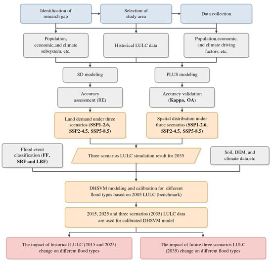
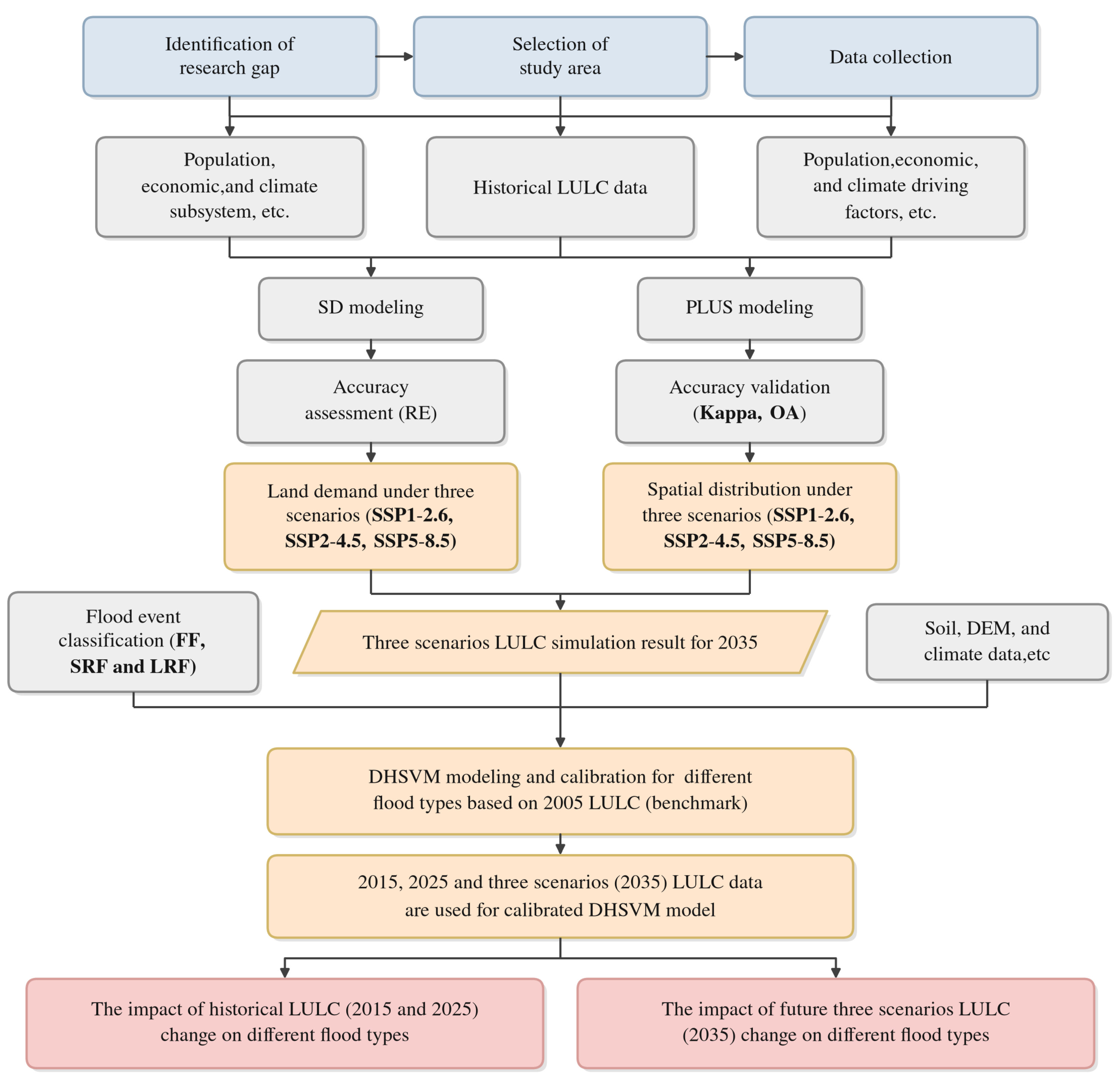
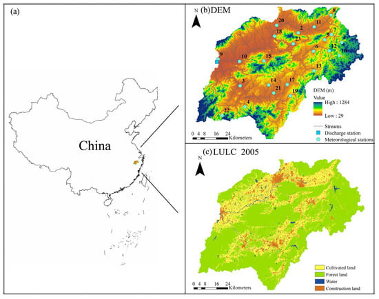
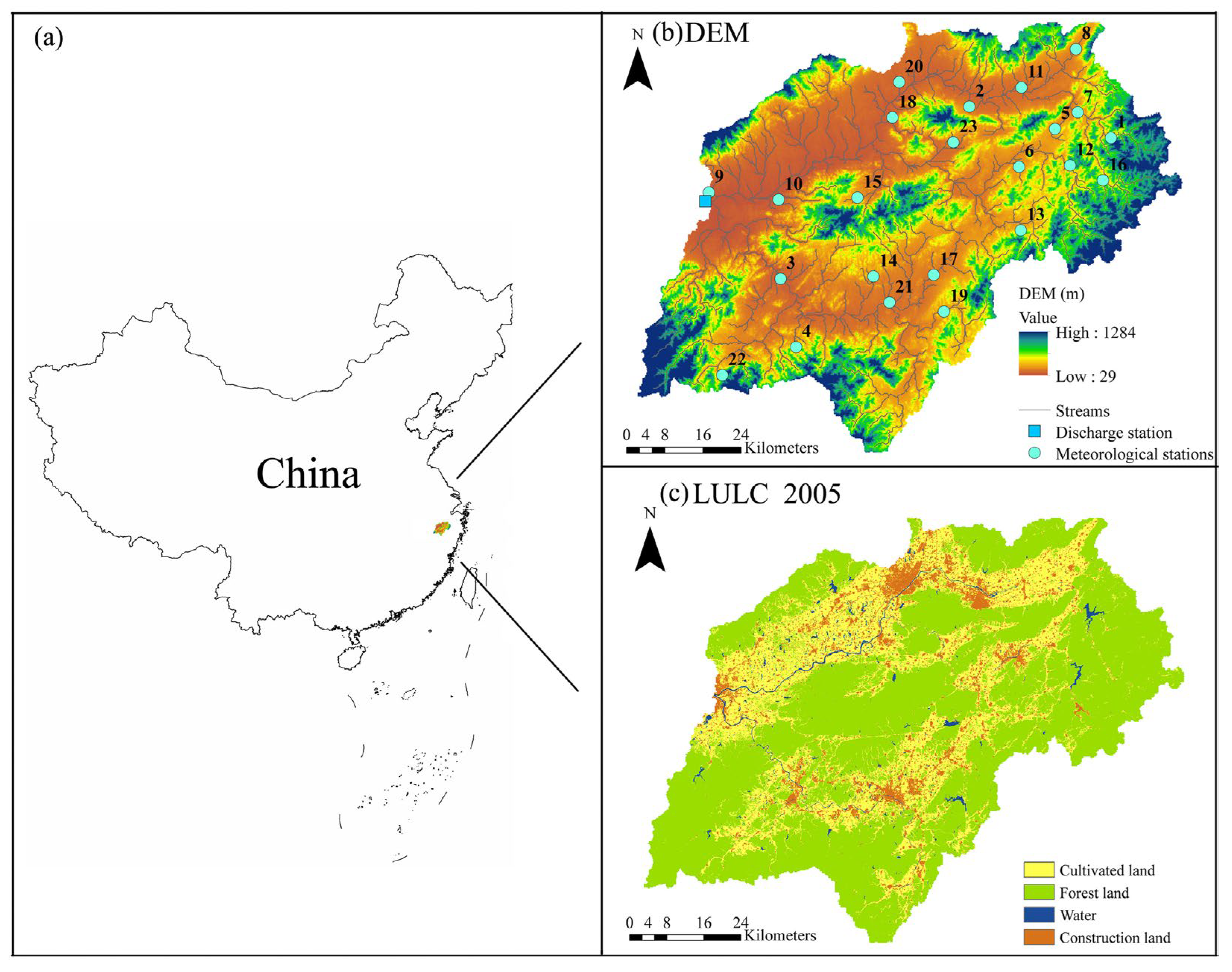
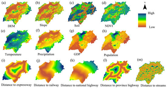
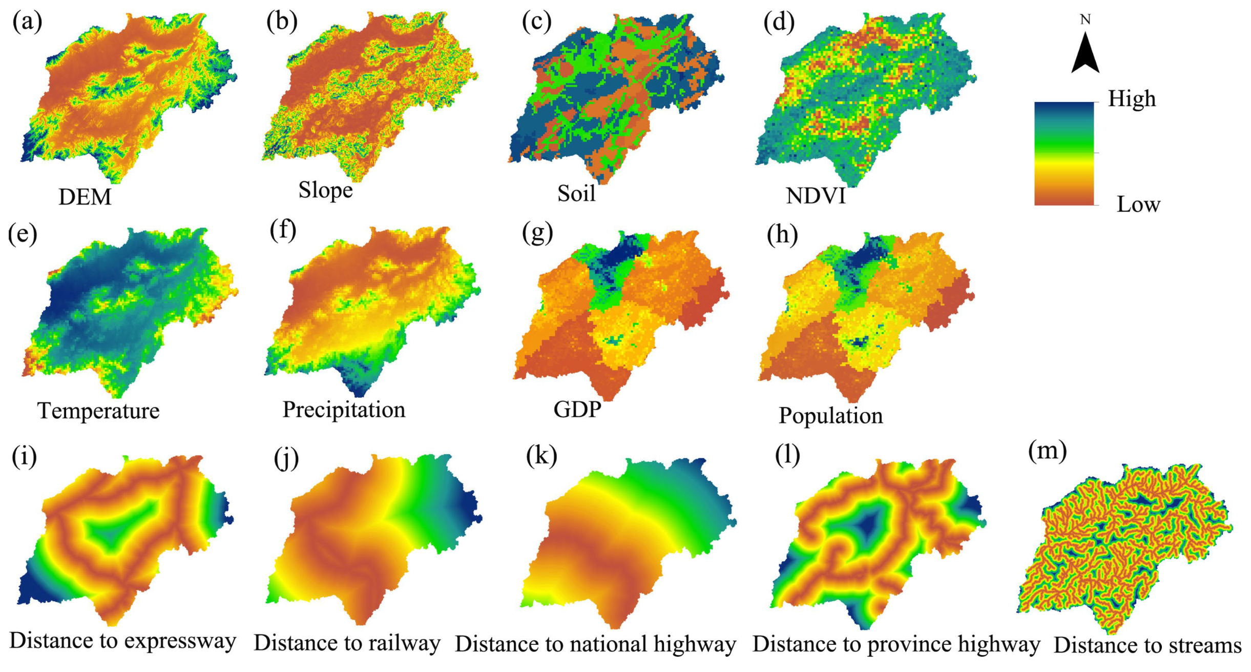
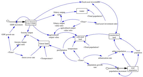
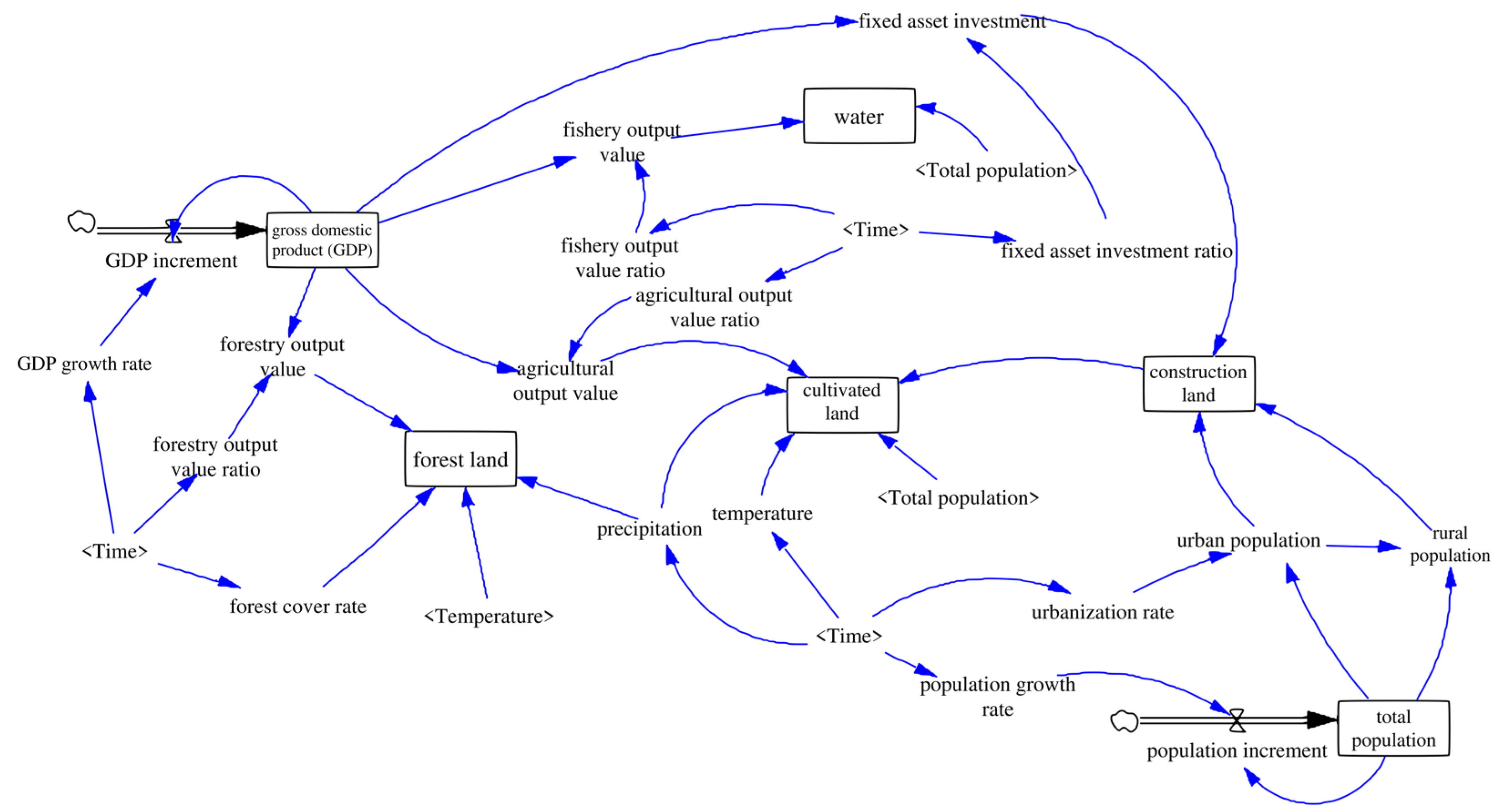
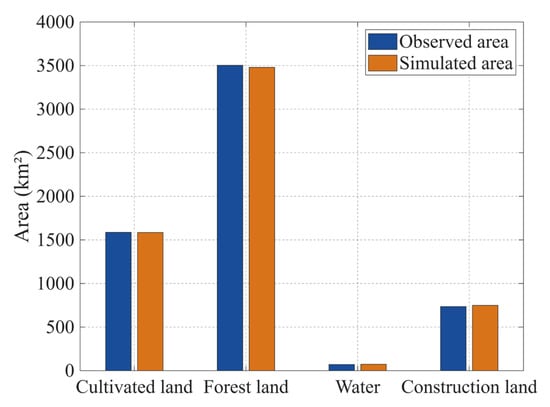
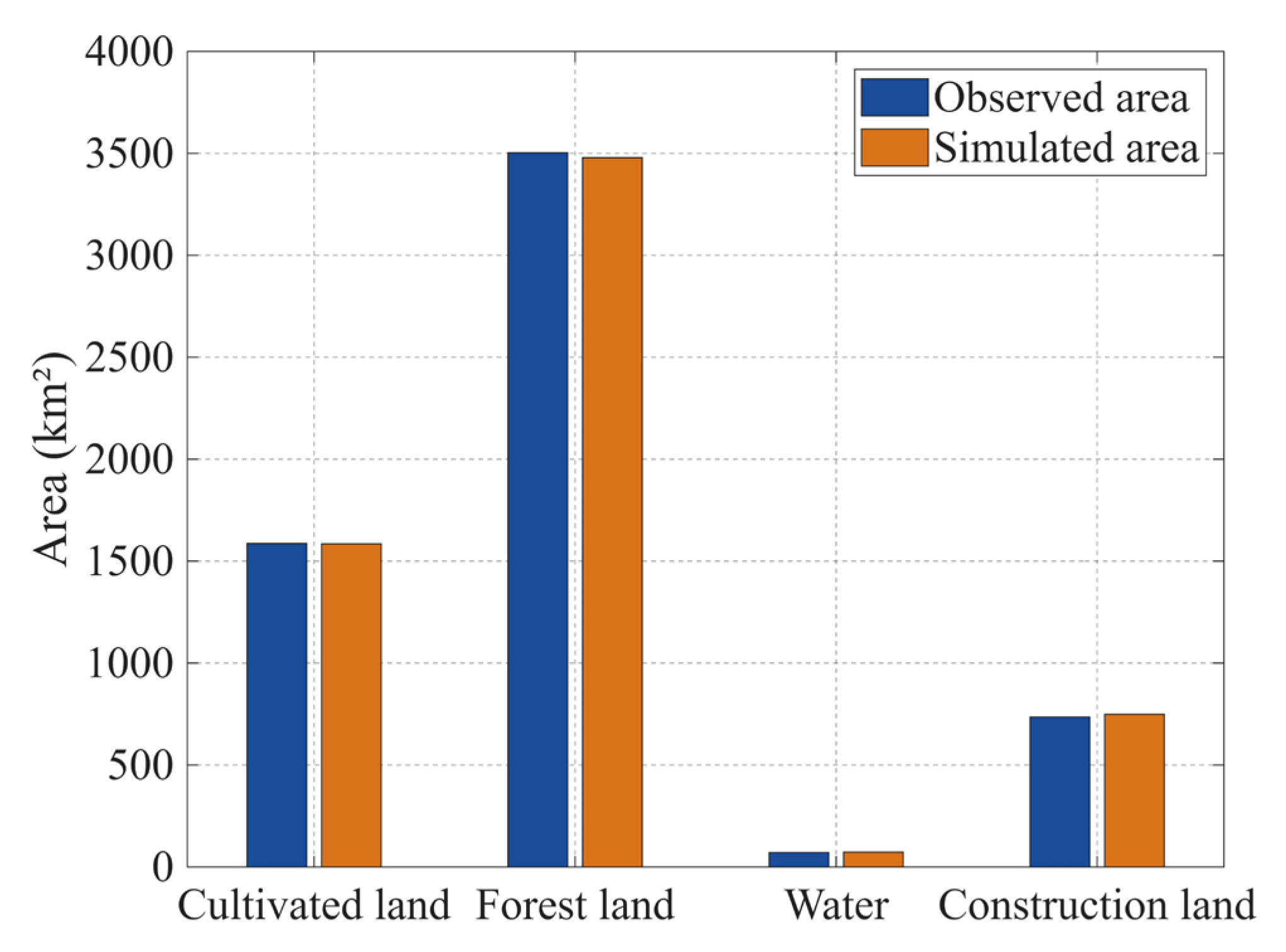
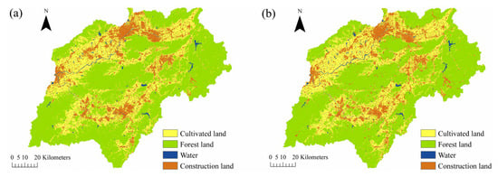
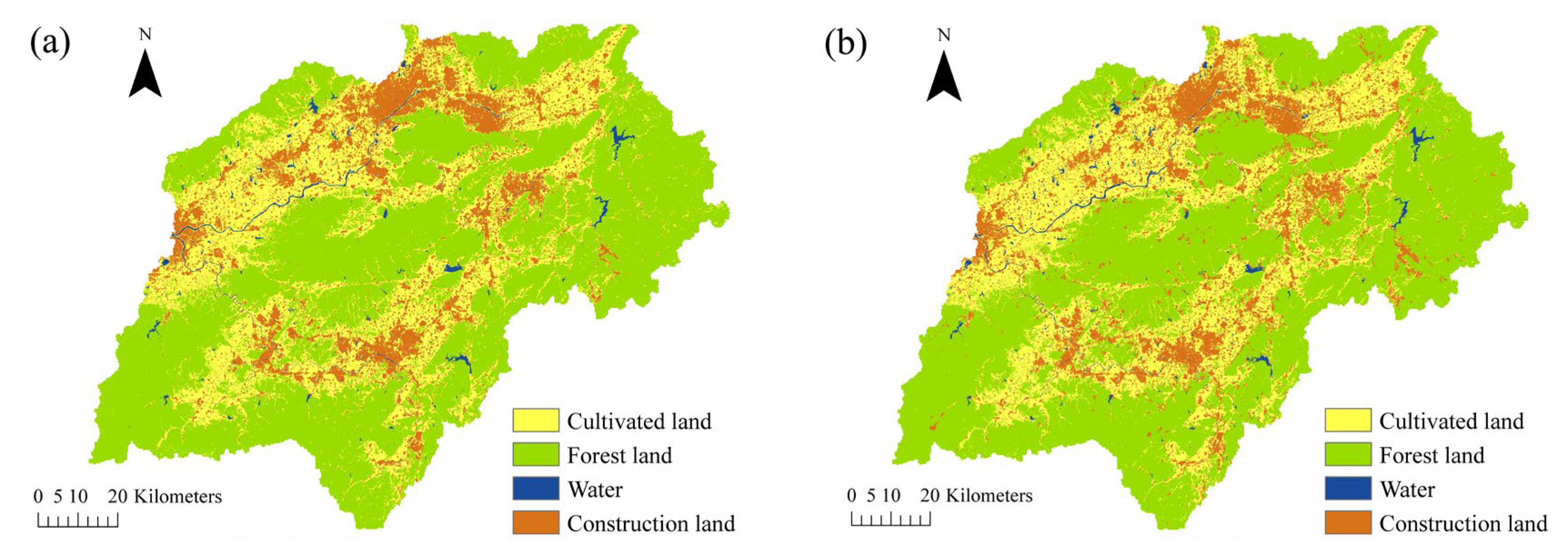
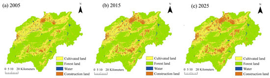
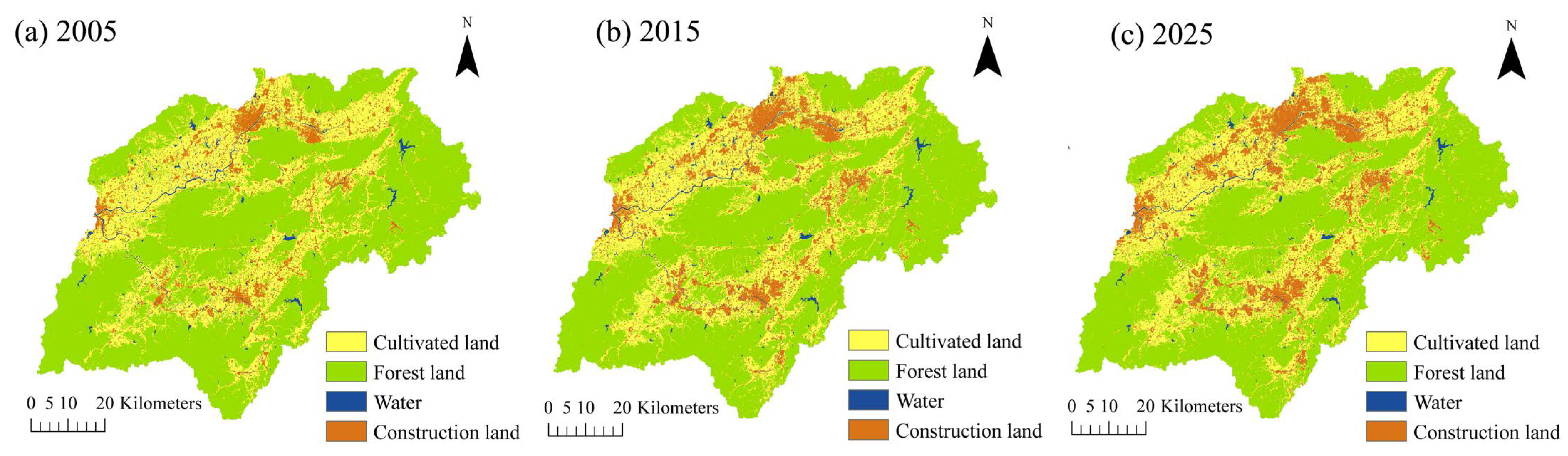
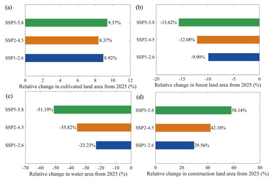
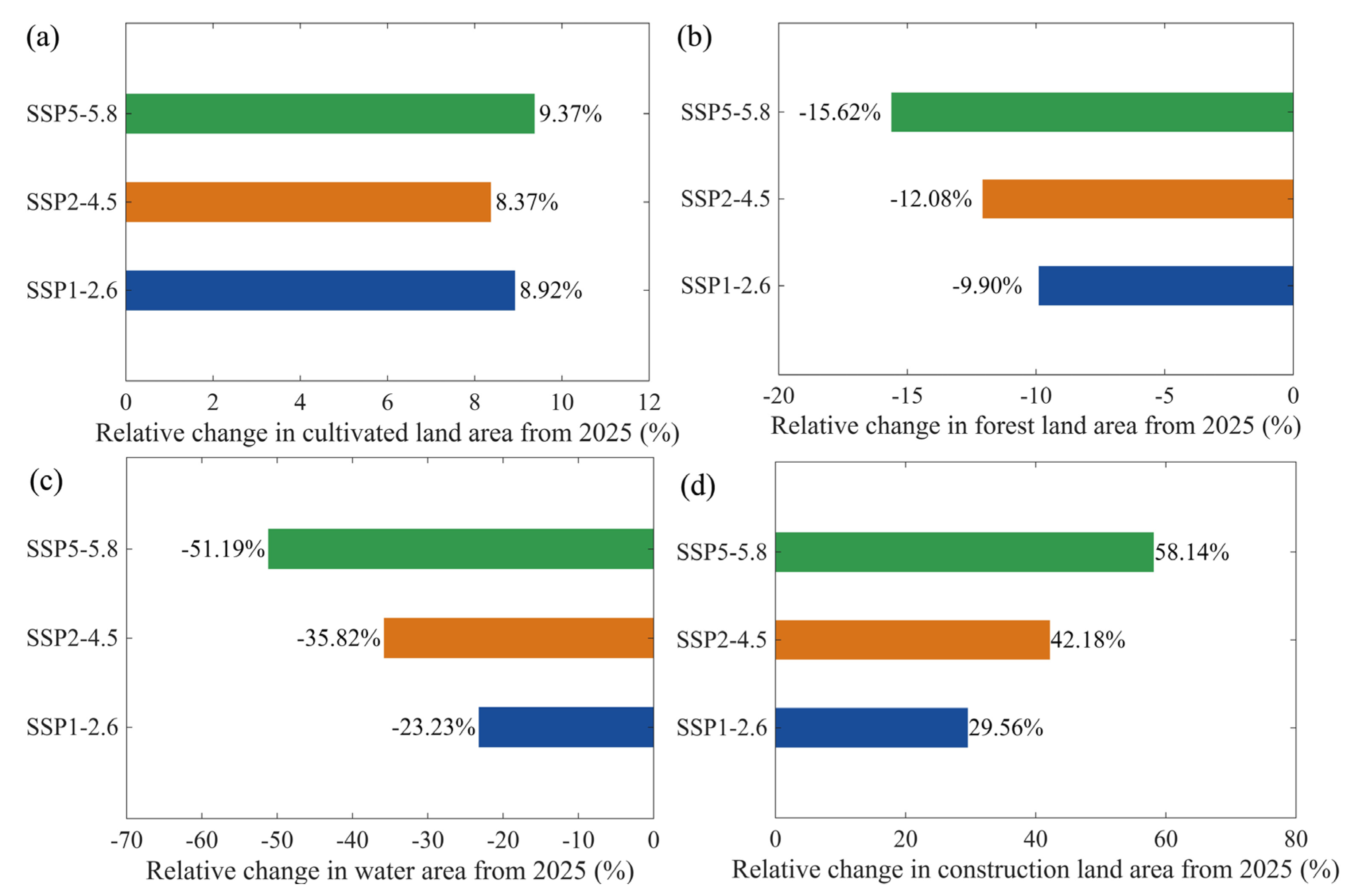
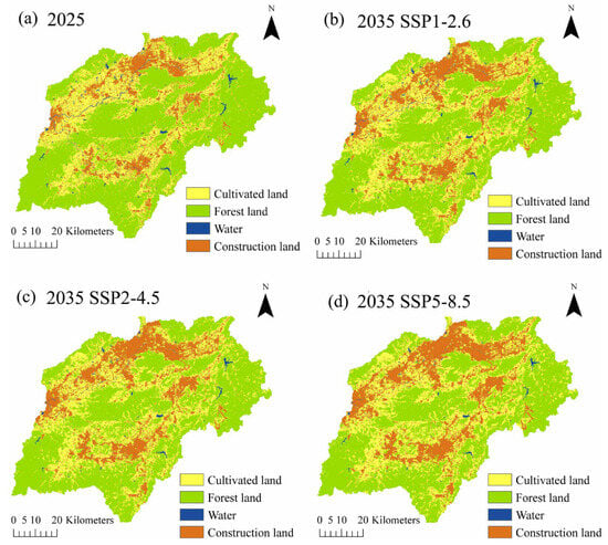
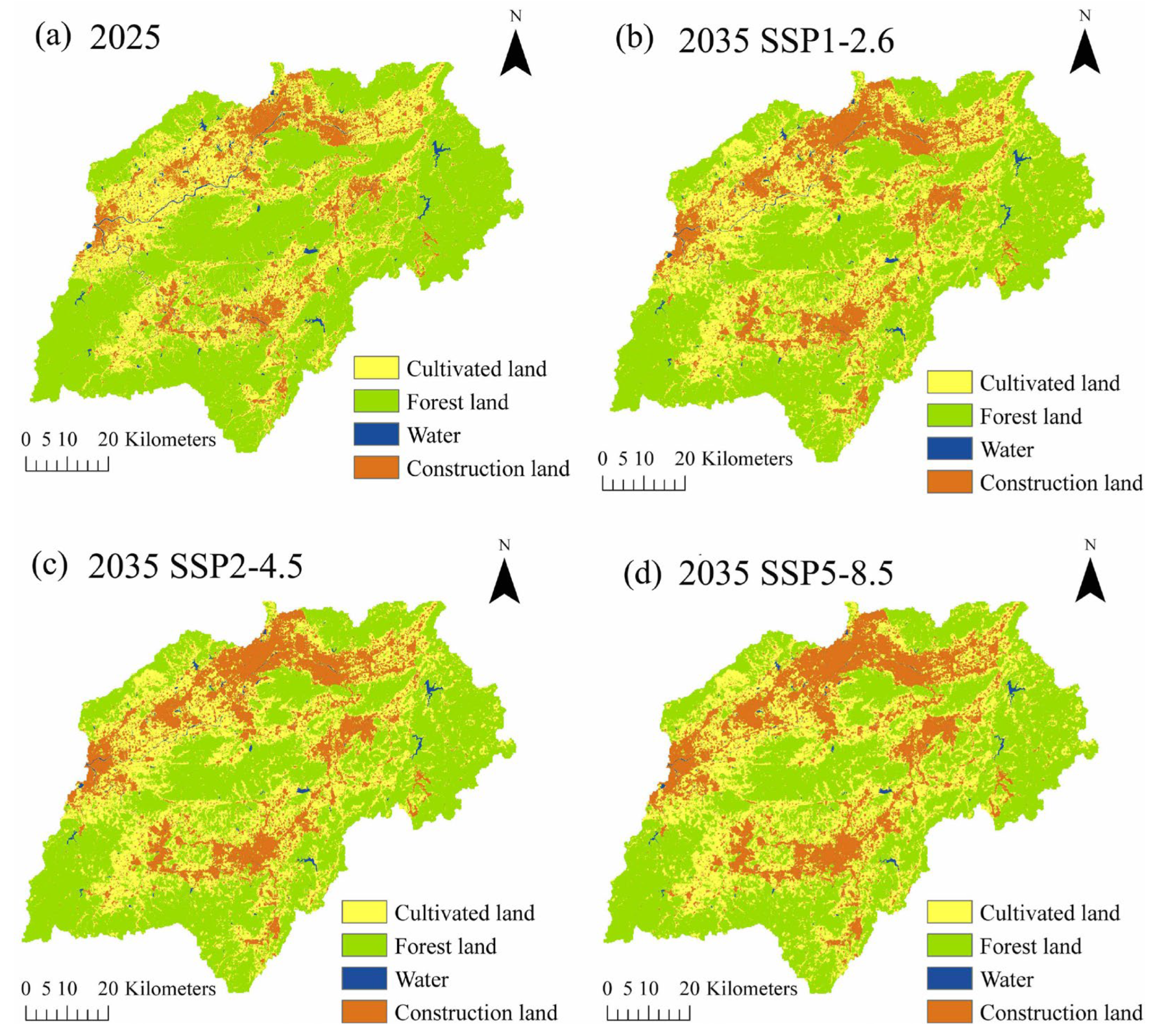
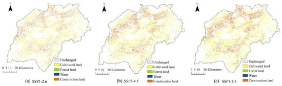
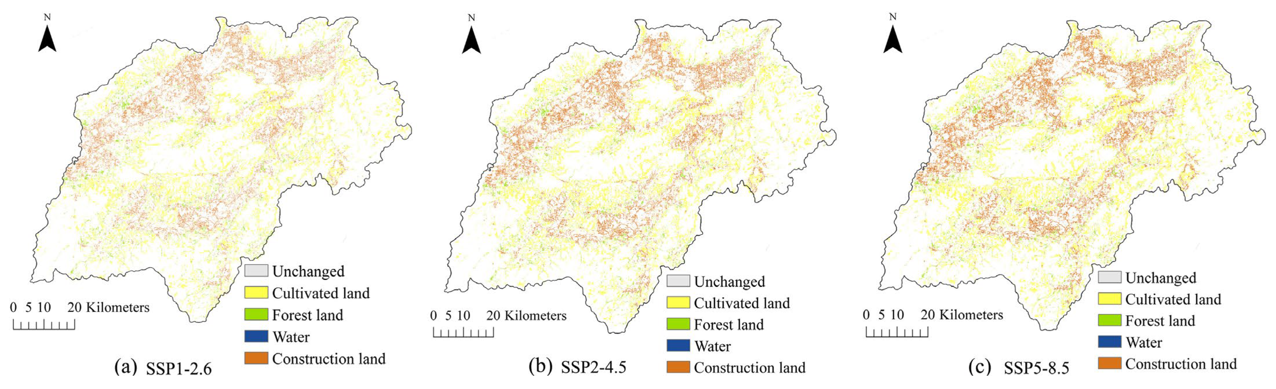
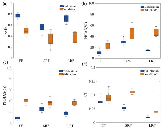
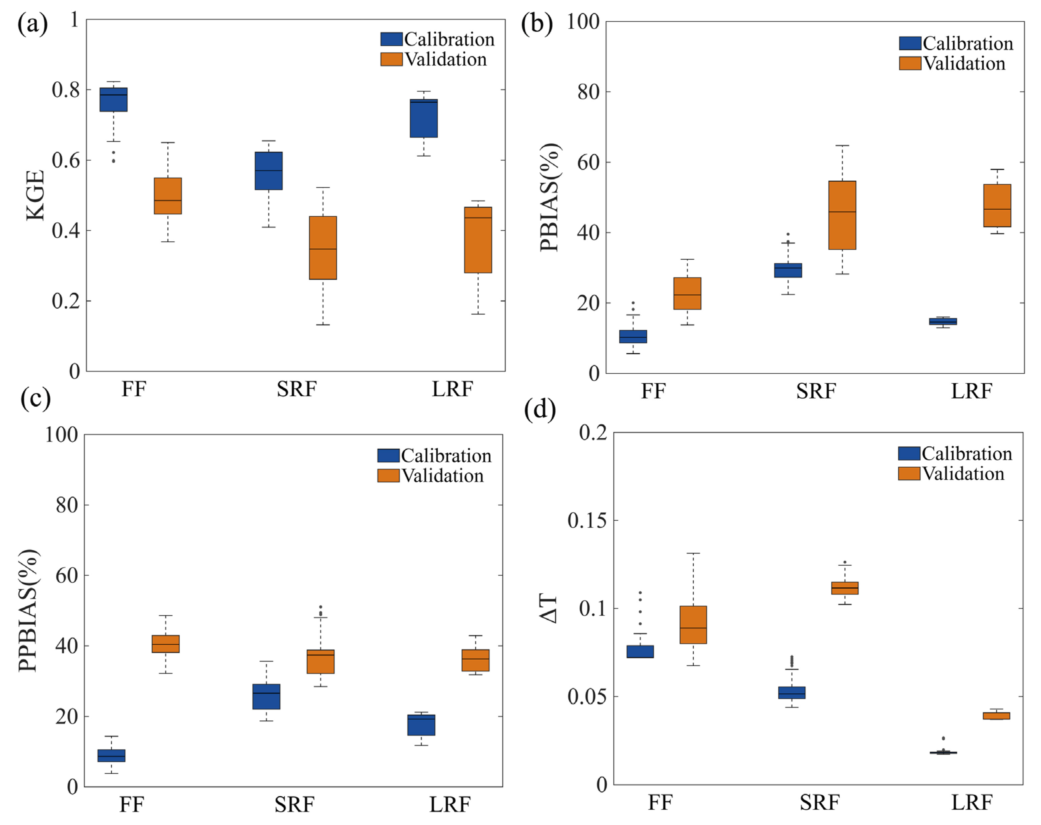
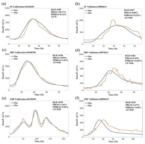
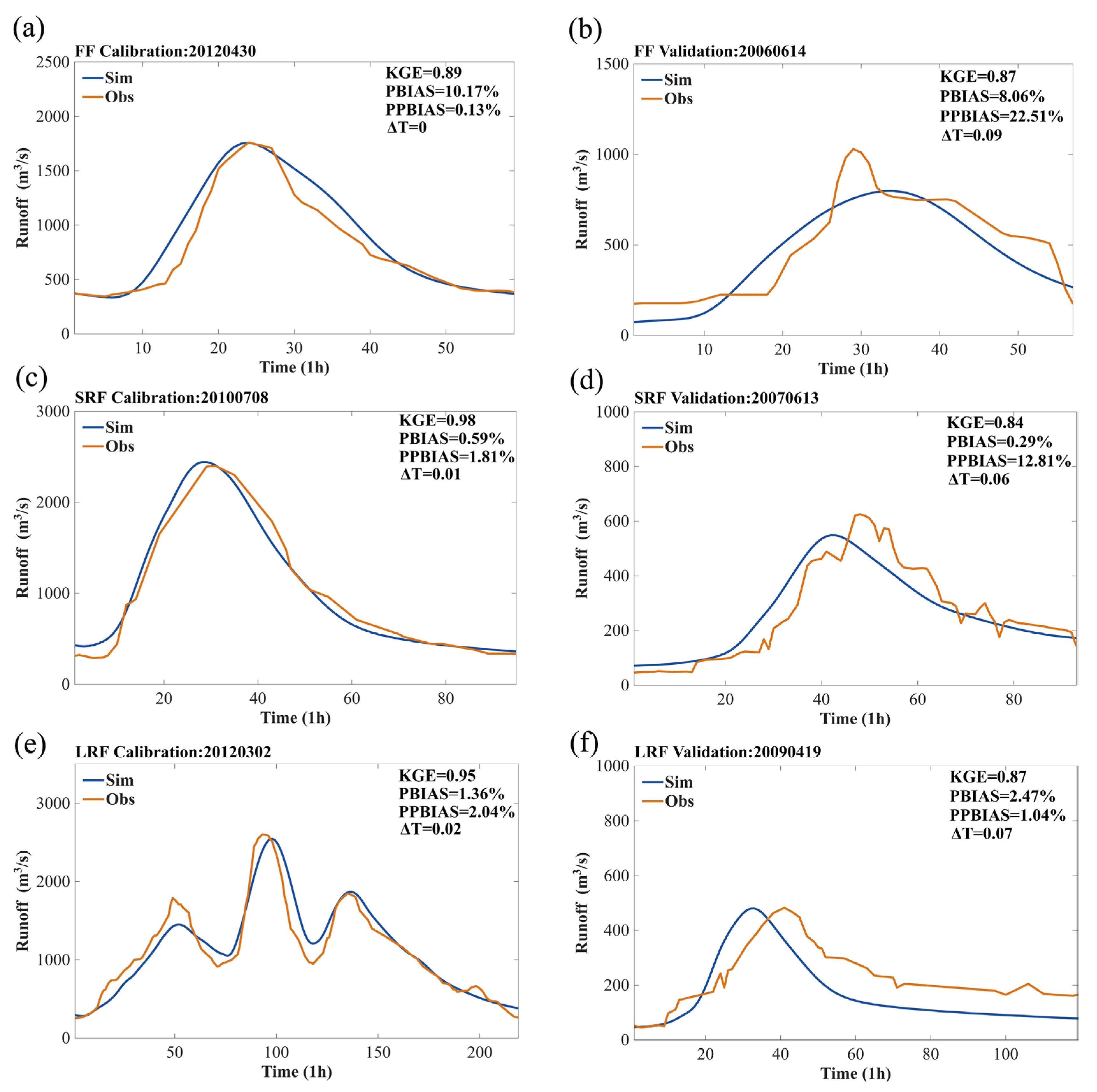
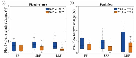
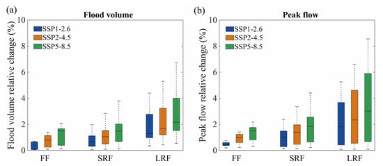

Disclaimer/Publisher’s Note: The statements, opinions and data contained in all publications are solely those of the individual author(s) and contributor(s) and not of MDPI and/or the editor(s). MDPI and/or the editor(s) disclaim responsibility for any injury to people or property resulting from any ideas, methods, instructions or products referred to in the content. |
© 2026 by the authors. Licensee MDPI, Basel, Switzerland. This article is an open access article distributed under the terms and conditions of the Creative Commons Attribution (CC BY) license.