Representation of Packed Log Jams in a Two-Dimensional Hydraulic Model

Abstract

Packed log jams (PWJs) can form naturally in streams and engineered log jams have been strategically placed in streams in river restoration projects. Their presence impacts stream hydraulics, flood inundation, morphology and ecology. Proper representation of large woods in two-dimensional hydraulic models is important, but proper guidelines are needed for any models, considering that such models have been widely used for assisting river restoration design and fish habitat evaluation. Existing large wood representation methods are inadequate. In this study, the porous-media method, widely used in groundwater modeling, is adapted and extended to represent large wood in streams. A modified formulation is proposed, which adopts only one calibration parameter to compute the drag force due to large wood presence. Two sets of experimental data with PWJs are used to assess the performance of the method. The porous-media method is found to produce good results when compared with the measured data of backwater rise as well as water depth and velocity variations along the flow. A general usage guideline is proposed on the proper way to apply the method and verified against the PWJ experimental data. Further, a regression equation is developed to estimate the large wood calibration parameter; it can be useful when no measured data are available for calibration. The proposed method, the developed guidelines, and the regression equation are found to produce satisfactory results in comparison with the measured PWJ data.

1. Introduction

Large wood structures (LWSs) form naturally in streams. They are widespread and have been found beneficial to river systems [1]. LWSs, therefore, have been widely used in river restoration projects worldwide [2,3].

Large wood (LW) presence may induce large impacts, good or bad, on flow processes due to much increased flow resistance [4]. They cause changes in flood stage, stream morphology and stream ecology [3,5]. For example, LWSs may raise the water stage, leading to increased flood risk [6,7]; stabilize stream channels [2,5]; alter local erosion and deposition, impacting sediment management [8,9]; and alter stream geomorphology [5,10,11]. There is also an urgent need to investigate the impact of multiple types of woody debris and vegetation on riverine property protections during floods [3]. Importantly, LW presence may result in ecological benefits—such as enhanced aquatic physical habitat [12,13,14], increased hyporheic flow exchange [15], and improved water quality [16].

Successful restoration projects rely on a good understanding of the relationship between LWSs, resultant hydraulic processes and eventual geomorphology. Numerical hydraulic models have generally been used to assist river restoration design due to complex interacting physical processes involved. Three-dimensional (3D) models may be more appropriate for some design questions [12,17,18,19]. In general, however, two-dimensional (2D) hydraulic models are often sufficient for answering most study questions [19] and more practical to use. 2D models have been widely used in understanding the impact of restoration changes on stream flow hydraulics and morphology [3,20,21,22].

The use of 2D hydraulic models with LWS presence, however, is challenging though widespread. In the past, LWSs have either been ignored or represented using simple methods such as a solid protrusion [23,24]. However, studies have shown that LWS properties such as porosity are significantly important and should not be ignored [23,25]. In [26], it was shown that neglect of LWS porosity could lead to 40% root-mean-square error in average stream velocity and 5% error in average water depth—both are important in computing habitat suitability indices in river restoration efforts. In another study, lack of proper accounting for the LWS presence resulted in erroneous hydraulic predictions at both reach and local scales [27].

As the importance of LWS inclusion in 2D models is increasingly recognized, several representation methods have been adopted (a review is provided below). This has led to a second challenge: a lack of a comprehensive evaluation of existing methods and a lack of general guidelines for their proper usage. Addy and Wilkinson [28] found that scientific knowledge remains an issue on the appropriateness of the existing LWS-representation methods. The suitability of each method has not been comprehensively evaluated [29], and there is a lack of accepted guidelines in the use of each method [30,31]. The review of [28] concluded that there was “a pressing need to assess the applicability of modeling to capture the hydraulic and hydrological effects of LW in rivers.” Sixta and Ubing [22] confirmed the limitations of existing methods and recommended the need for further study.

The current state-of-the-practice leads to the primary objective of the present study: the development of an LWS-representation method in a 2D hydraulic model, along with the development of general usage guidelines. A key aim is to ensure that 2D models may be applied properly and satisfactorily for river restoration applications.

2. Scope

LWSs may be formed naturally due to fallen trees, logs and stumps, or be manually installed by humans or other actors. Three general LWS categories may be distinguished: packed wood jams (PWJs), engineered log jams (ELJs) and loosely distributed large wood (LDLW). In this study, PWJ is the primary focus; research into the ELJ type is in progress and will be reported in the future.

PWJs, formed mostly by floating woody debris during floods or by beavers, are defined as woody debris that is active and leaky and induces a backwater rise upstream. PWJs may extend across the entire stream (named channel-spanning PWJs in this study) or only a part of the stream width (named partial-spanning). Extensive experimental studies have been carried out in recent years by [32,33]—the measured data are reported in [34,35]. In recent years, PWJs have also been actively investigated numerically by, e.g., [36,37]. Altmann et al. [36] proposed a new yet simple PWJ-representation method in a 2D model to simulate the laboratory cases of [32,33]. The model was found to predict the PWJ-induced backwater rise within 30% of the prediction range. Radiyan and Liu [37] have also carried out laboratory experiments with PWJs’ presence to evaluate the importance of flow conditions and sediment transport. They additionally conducted 2D numerical modeling of the measured cases to evaluate the existing LWS-representation methods. They concluded that two widely used existing methods produced good results only when they were recalibrated if flow or sediment conditions changed.

In the following, a literature review is first provided with the existing LWS-representation methods, and discussion focuses on their pros and cons. The proposed representation method is then presented. The method is evaluated in two stages: using a partial-spanning dataset of [33] first and channel-spanning cases of [32] next. Finally, guidelines are proposed and evaluated, and a regression equation is developed to estimate the calibration parameter for the PWJ type.

3. A Literature Review

Flows with instream LWSs have been widely simulated using 2D hydraulic models, and various methods have been applied. An extensive study was reported by Sixta and Ubing [22]. Several methods, available in the SRH-2D model [38], were evaluated for a field case; the objective was to determine the best methodology. Based on sensitivity analyses, they found that no existing method was adequate, at least for the case studied. Reviews of the existing methods have also been reported by others, including [28,32,39]. In the following, the existing methods are categorized into five types, and each is discussed.

3.1. Solid-Block Method

The solid-block method represents the LWS by modifying the stream bed terrain to account for the LWS’s presence—a method recommended by [40,41]. This is one of the simplest methods, as it is transferable across all existing 2D models without the need for model modifications. In Sixta and Ubing [22], the solid-block method was achieved by treating the LWS as a fully blocked obstruction, i.e., the bed elevation of the mesh was raised to the design elevation of the LWS’s top surface.

Despite its simplicity, there is a severe limitation with the method: LWS permeability is omitted, and the method has been found to overestimate the flow resistance unless it is artificially compensated by reducing the total blockage volume. Manners et al. [23] reported that the drag force was overestimated by 10–20% and the maximum bed shear stress was overpredicted by 75% for the bank-attached LWS case simulated. Addy and Wilkinson [28] suggested that the solid-block method, along with the partial-block method discussed below, might produce reasonable predictions of the hydrograph shape [42]. The flow hydrograph, however, was unrealistically delayed. The study in [22] showed that the solid-block method produced poor results in comparison with other methods and was not recommended for general use.

3.2. Partial-Block Method

The partial-block method is an alternative to the solid-block method. It attempts to add the permeability of the LWS—achieved by dividing the LWS into columns of solid bars. However, the method achieved partial blockage only through a refined mesh, as a portion of the mesh was used to represent the solid columns.

The limitation of this method is obvious: it is difficult to determine the appropriate level of the blockage (e.g., the proper number of solid columns), and a much-refined mesh is needed to allow flows through the voids. In addition, various ways of solid-void partitioning are possible and hard to determine. LWS representation can be challenging in practical applications. The partial-block method was evaluated by Sixta and Ubing [22]; a sophisticated block-defining method was also proposed in [36]. Sixta and Ubing [22], based on the field application, did not recommend the method due to its arbitrary nature and inconsistency in repeating the simulation under different conditions. Under laboratory conditions, Altmann et al. [36] achieved satisfactory results when a particular way of partitioning was followed and additional LWS-induced friction was added.

3.3. Manning’s Equation Method

The Manning’s equation method is a straightforward way to take into account the LWS-generated drag force. With this method, a horizontal zone is delineated to represent the LWS footprint, and the Manning’s coefficient is then artificially increased within the zone to represent the drag force. The method was recommended by, e.g., [28,42]. The method is attractive, as the Manning’s equation has already been utilized in existing 2D models for bed friction, so no additional model development is needed.

Despite its simplicity, however, the method is less likely to be general, as it lumps together the LWS drag force with bed friction and other energy losses. Sixta and Ubing [22] showed that the method was effective in reproducing the backwater rise by LWSs but produced unsatisfactory velocity distribution. The method would also generate anomalous results for the bed shear stress and stream power that were often used for sediment analyses. Addy and Wilkinson [28] concluded that “there are important transferability and spatiotemporal limitations to be aware of” with the method. Another drawback is that no general guidelines have been developed, to my knowledge, to select the appropriate Manning’s coefficient for a given LWS; it has been found dependent on flow conditions in the literature (see the wide range of roughness values reported in Table 2 of [28]). This flow-dependency means a calibrated roughness coefficient under a steady flow may not provide a valid prediction for different flows or under unsteady conditions.

3.4. Drag-Force Method

With the drag-force method, the LWS-generated resistance force is explicitly computed using the well-known equation relating the drag force to the flow velocity and projected LWS area. This method has been incorporated in an SRH-2D model [38] and used in applications [22,37].

The drag-force method has the benefit of a clear physical meaning based on fluid mechanics, and the LWS resistance force is computed separately from the stream bed friction. However, studies have shown that the method is not more general than the Manning’s equation method, at least for flow simulations. In a field application of the two methods, Sixta and Ubing [22] found that the drag-force method produced only slightly better velocity patterns, but the differences were small. Lai et al. [19] showed that the two methods needed to go through the same calibration process and produced similar results. In a recent study, Radiyan and Liu [37] showed that the two methods were equivalent and a simple conversion relation existed between the drag coefficient and Manning’s coefficient if the LWS footprint was a rectangle. An important conclusion was that the drag coefficient value varied under different flow conditions, making the development of guidelines difficult.

3.5. Mixed Method

The mixed method refers to the use of a combination of the above four methods. For example, the method reported by Altmann et al. [36] may be classified as a mixed method, a combination of the partial-block and Manning’s equation methods. This study attempted to take into account two distinctive PWJ effects: flow blockage by PWJ logs and energy loss by log surface friction. The Altmann study demonstrated that a mixed method might obtain reasonable results. The mixed method of [36], however, has its drawbacks despite success. First, a strategy is required to determine the solid-void partition—a challenging task as discussed before. Second, the partition needs to be represented by a much-refined mesh, which needs to be changed if the porosity changes. Lastly, more than one physical process needs to be calibrated: the flow constriction due to LWS porosity and energy loss for the flow through the PWJ.

3.6. Discussion of Existing Methods

The existing methods have achieved some success when measured data are available for model calibration. This success, however, may be case-dependent. As a result, no general guidelines have been developed, probably due to the non-general nature of the methods. The state-of-the-art review in [28] may be quoted as a summary: “Despite the number of studies and range of methods applied, most are heuristic in nature and quantitative validation of approaches has been limited.”

Some of the shortcomings of the existing methods are summarized below:

• Lack of rationale why a particular LWS-representation method should be selected—an outcome of a lack of verification and validation;
• Lack of useful and practical guidelines to select and apply a particular method;
• Little attention has been paid to the importance of LWS porosity and drag-coefficient-based methods [28];
• Little attention has been paid to the importance of LWS types as well as the LWS scale effect [28].

The above review points to the need for more studies on an appropriate LWS-representation method. This study’s objectives now can be summarized: (a) development of a defensible LWS-representation method that takes into account the LWS type and porosity; (b) verification/validation of the proposed method for the PWJ type; and (c) development of general guidelines in applying the method. The LWS scale effect is not tackled in this study, as it is more appropriate to use 3D CFD models for such a study.

4. Proposed LWS-Representation Method

In this study, a different LWS-representation method, named the porous-media method, is proposed and evaluated for use in 2D hydraulic models. This study consists of two steps. First, the porous-media method widely used in groundwater modeling is extended and evaluated. This study seeks a method valid over a range of flow discharges and stages once a key model parameter is calibrated under one steady flow condition. A general guideline is also developed based on a comparison with the measured PWJ data. It has been known that the resistance force coefficient depends on both flow conditions and the LWS’s geometric features in addition to stream characteristics and LWS blockage ratio. It is probably not feasible to develop a method that may incorporate all the above features [37], but the limitations need to be understood. In the second step, an empirical relation, based on PWJ data, is developed to estimate the calibration parameter when no measured data are available.

Note that this study is limited to the PWJ type. This restriction is due to limited availability of measured data for other LWS types. Indeed, the porous-media method itself may be applicable to other types. Its appropriateness, however, can only be evaluated in the future when reliable data becomes available.

4.1. Governing Equations

Stream flows are governed by the St. Venant equations, which may be derived under the shallow-water assumption and by depth-averaging the 3D flow equations. The governing equations represent the mass and momentum conservation laws and may be expressed in tensor form as [38]:

$${\displaystyle \frac{\partial ph}{\partial t}}+\nabla •(h\overrightarrow{\mathit{V}})=0$$

(1)

$${\displaystyle \frac{\partial \left(ph\overrightarrow{V}\right)}{\partial t}}+\nabla •\left(h\overrightarrow{V}\overrightarrow{V}\right)=-p^{2}gh\nabla Z+\nabla •\left(h\overrightarrow{\overrightarrow{T}}\right)-{\displaystyle \frac{{\overrightarrow{\tau }}_b}{\rho }}-p^{2}h{\displaystyle \frac{\overrightarrow{F_R}}{\rho }}$$

(2)

In the above, t is time, h is water depth, $\overrightarrow{\mathit{V}}$ is depth-averaged horizontal velocity vector, Z is water surface elevation, $\overrightarrow{\overrightarrow{\mathit{T}}}$ is 2nd-order tensor representing turbulence and dispersive stresses, ${\overrightarrow{\mathit{\tau }}}_{\mathit{b}}$ is bed shear stress, $\rho$ is water density, and $\overrightarrow{F_R}$ is LWS-generated resistance force (the total force exerted on water by the LWS). A special variable p, the LWS porosity, appears explicitly in the above equations—it assumes the value of unity (1.0) in flow areas without the LWS but less than 1.0 in the LWS footprint. Refer to [38] for a detailed expression of $\overrightarrow{\overrightarrow{T}}$ and Manning’s equation to compute the bed shear stress ${\overrightarrow{\mathit{\tau }}}_{\mathit{b}}$. In addition to porosity, only the flow resistance force $\overrightarrow{F_R}$ is a new term and discussed below.

4.2. Resistance Force Method

The flow resistance force $\overrightarrow{F_R}$ may be computed using any of the existing methods reviewed above. Herein, the drag-force method is discussed first, and the proposed porous-media method is presented next.

The drag-force method computes $\overrightarrow{F_R}$ by resorting to the classic drag force equation in fluid mechanics. For each LWS, a horizontal footprint is delineated, representing the LWS’s spatial extent; the total flow resistance in the zone is then computed as:

$$\overrightarrow{F_R}={\displaystyle \frac{A_{LW}}{2{\forall }_{LW}}}{C}_R\rho \left|\overrightarrow{V}\right|\overrightarrow{V}$$

(3)

In the above, C_R is the resistance coefficient, ${\forall }_{LW}$ is the volume occupied by the LWS, and A_LW is the LWS projected area. Note that local bulk velocity ($\overrightarrow{V}$) is used in place of the upstream approach velocity. For this reason, the above resistance force formula is not the same as the classic drag force equation, as local bulk velocity is typically much smaller than the approach velocity. As a result, the value of C_R is quite different from and much larger than the classic drag force coefficient reported by, e.g., [23,43,44]. In implementation, the total resistance force is distributed to mesh cells occupied by the LWS footprint. In applications, C_R is treated as a calibration constant. Reported C_R variation has been between 10 and 70 for a wide range of flows, but no general guidelines have been developed.

In this study, the porous-media method, widely used for groundwater flow modeling, is adapted and extended to simulate flows through the LWS within 2D hydraulic models. This means the flow through an LWS is treated as a special type of porous-media flow. To my knowledge, such an extension has not been reported in the literature with 2D models. The porous-media method, however, has been adopted in coastal engineering to simulate porous structures by, e.g., [45,46]. It was also explored in a 3D CFD model for flows through an LWS in [17]. The Xu-Liu study found that the porous-media method could yield good results in the far-field and even reasonable results in the near-field and wake regions.

In this study, the governing equations of van Gent [45] are extended to flows with an LWS presence; they are expressed in Equations (1) and (2). These resemble the standard shallow-water equations, except that LWS porosity is explicitly added and the resistance force ($\overrightarrow{F_R}$) is added. Note that within the LWS footprint, $\overrightarrow{V}$ is the depth-averaged bulk velocity, not the actual flow velocity.

Following the groundwater model of van Gent [45], the resistance force $\overrightarrow{F_R}$ is computed according to the Darcy–Forchheimer equation as:

$$\overrightarrow{F_R}=\rho \alpha {\displaystyle \frac{{\left(1-p\right)}^2}{p^3}}{\displaystyle \frac{\nu }{{D_L}^2}}\overrightarrow{V}+\rho \beta {\displaystyle \frac{(1-p)}{p^3}}{\displaystyle \frac{1}{D_L}}\left|\overrightarrow{V}\right|\overrightarrow{V}$$

(4)

where $D_L$ is the porous-media grain diameter for groundwater flows but represents an LWS length scale (called log size), and $\alpha$ and $\beta$ are two dimensionless parameters.

It is seen that three parameters are needed with the above equation: ELJ log size $D_L$ and dimensionless parameters $\alpha$ and $\beta$. In this study, only one calibration parameter is sought so that the method may be practical in real-life applications. Past porous-media modeling studies have already determined a proper range for $\alpha$ and $\beta$. For example, $\alpha =1000$ and $\beta =1.1$ were determined by [45], while $\alpha =200$ and $\beta =2.0$ were recommended by Jensen et al. [46]. For flows through the LWS, 3D CFD modeling was reported in [17], using the same porous-media method—it was found that the values of van Gent [45] provided better results. The present study, therefore, follows [17] by fixing $\alpha =1000$ and $\beta =1.1$. Two reasons are offered for the choice: (1) these values were verified to be good for flows through an LWS, although a 3D model was applied; (2) it is the ratio of the two parameters that is more important, as absolute values may be adjusted through the LWS coefficient to be discussed below; note that the ratio is similar between [45] and [46] despite the absolute value difference. It is acknowledged that use of fixed $\alpha$ and $\beta$ values makes the model less flexible in calibration; however, the benefit outweighs the restriction: only one parameter needs to be calibrated in applications. Further, a dimensionless parameter, named the LWS coefficient (${\alpha }_{log}$), is defined in this study to represent the log size and serves as the calibration parameter. The relationship between the log size and the LWS coefficient is $D_L={\alpha }_{log}{d}_{log}$ (where $d_{log}$ is the average LWS log diameter). In this formulation, the log size $D_L$ has a physical meaning: it should resemble the “grain diameter” of a porous media for groundwater flows. Therefore, it is expected that $D_L$ is similar to the log diameter ($d_{log}$); therefore, the LWS coefficient (${\alpha }_{log}$) is expected around a value of 1.0—a hypothesis to be verified. Note that the mean log diameter is readily measurable in the field.

It is commented that the two terms of the resistance force in Equation (4) have their physical representations. The linear term is related to the skin friction of the LWS, while the quadratic term is due to the form drag generated by the logs. In the context of groundwater flows, the linear term dominates as flows are usually slow and laminar since ground media diameter is mostly fine-grained and small; the quadratic term, on the other hand, becomes important only when the flow is turbulent, which is primarily associated with coarse-grained media.

The limitations of the proposed method need to be noted. LWS properties are assumed uniform within the footprint, and resistance force is implemented in a 2D depth-averaged fashion. The method aims to correctly represent the obstruction effect on flows away from the LWS. Local flow details such as velocity magnitude may not be accurate within the LWS footprint—therefore, near-field flow results should not be used to draw design conclusions. For such a purpose, detailed 3D modeling is recommended, such as in [17,19]. Results immediately downstream of the LWS may also be inaccurate if the backwater rise is significant due to the depth-averaged nature [37].

5. Results and Discussion

The proposed porous-media method is evaluated using experiment data with flows through PWJs. Note that the experiments are not part of this study and were carried out by others as described below.

5.1. Partial-Spanning PWJs

Partial-spanning PWJs were studied by [33] with a series of experimental tests. This dataset is valuable as both water depth and flow velocity profiles were measured along longitudinal transects of the flow, not just the backwater rise.

5.1.1. About the Experiment and Numerical Model

A series of flume experiments were conducted with partial-spanning PWJs by [33]—a total of 20 cases. The flume was 10.7 m long, 1.0 m wide, and 0.8 m deep and had a flatbed that could be tilted. The flume inlet section was equipped with a flow straightener to create uniform approach flows, and the side walls were made of glass and PVC. The stage at the flume exit was controlled by a flap gate and varied around 0.2 m.

Partial-spanning PWJs, though a few were channel-spanning, were placed within two aluminum racks, which were 4.0 m downstream of the flume inlet and had a longitudinal length of 0.2 m. The PWJ was constructed from natural woody logs with the following properties: (a) log diameter 0.027 ± 0.003 m; (b) log length 0.25 ± 0.01 m; and (c) PWJ height 0.34–0.49 m. Two PWJ properties were varied. One was the PWJ lateral width called blockage; it varied between 0.25 and 1.0 m, leading to a blockage of 25%, 50%, 75%, 90% and 100%, respectively. Another was the PWJ porosity, which varied between 0.49 and 0.8; most had a porosity of 0.6.

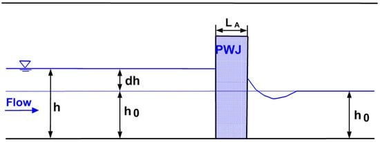
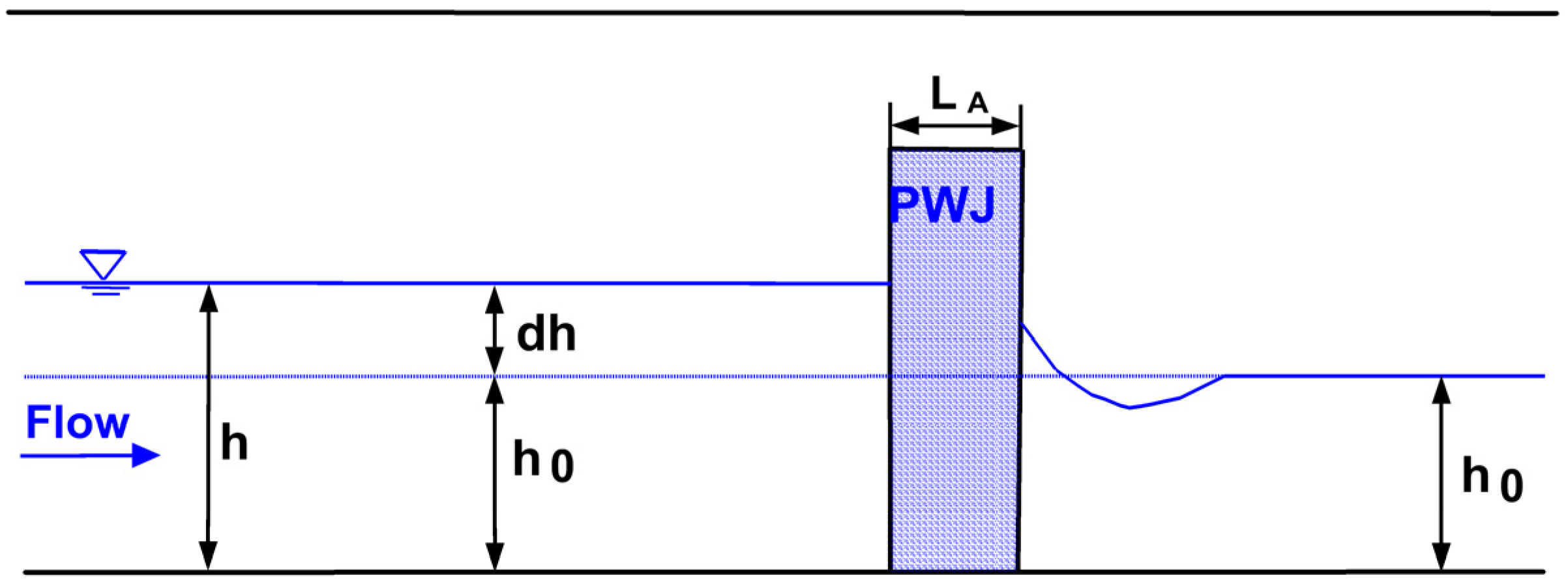
The flow conditions primarily varied in discharge. The uniform upstream flow had an approach velocity between 0.1 and 0.8 m/s, leading to the Froude number from 0.1 to 0.6. Some had supercritical flows in the PWJ gap zone. An illustrative side view of the flume setup is shown in Figure 1.

Figure 1. Illustrative side view of the flume setup for both partial- and channel-spanning PWJ experiments.

The relevant parameters of the dataset are documented in Table 1. This dataset is valuable in evaluating the performance of the LWS-representation method and used to assess effects of flow discharge and PWJ blockage. The importance of other properties, such as flow stage and PWJ porosity, will be addressed later with the channel-spanning dataset.

Table 1. Major parameters of the 20 cases with the experiment of [33].

Case ID	Discharge (m3/s)	Froude Number	PWJ Blockage	PWJ Porosity	${\mathit{h}}_0$ (m) Measured
1	0.02	0.07	100%	0.6	0.24113
2	0.02	0.07	100%	0.5	0.22981
3	0.02	0.07	100%	0.8	0.20728
4	0.02	0.07	90%	0.61	0.21237
5	0.06	0.21	90%	0.61	0.28333
6	0.10	0.36	90%	0.61	0.36247
7	0.20	0.07	75%	0.6	0.20544
8	0.10	0.36	75%	0.6	0.29332
9	0.159	0.57	75%	0.6	0.37215
10	0.02	0.07	50%	0.6	0.20272
11	0.06	0.21	50%	0.6	0.21357
12	0.10	0.36	50%	0.6	0.23541
13	0.159	0.57	50%	0.6	0.29394
14	0.02	0.07	25%	0.58	0.20092
15	0.10	0.36	25%	0.58	0.20904
16	0.159	0.57	25%	0.58	0.24404
17	0.02	0.07	50%	0.49	0.20323
18	0.06	0.21	50%	0.49	0.21454
19	0.10	0.36	50%	0.49	0.22311
20	0.06	0.21	50%	0.79	0.21449

The 2D model domain is rectangular and has a longitudinal length of 7.0 m and lateral width of 1.0 m. PWJs have a fixed longitudinal length of 0.2 m and are placed 3.0 m downstream of the inlet. A mesh of 7140 cells is used and found fine enough for this study. The mesh has 170 cells longitudinally and 42 cells laterally, with a finer resolution within and near the PWJ. A total of 15 longitudinal cells is within the PWJ. This mesh resolution is in agreement with the recommendation by [37], who found that at least five longitudinal cells were needed within a PWJ to achieve mesh-independent results.

The reported flow discharge is imposed as the inlet boundary condition for all simulations (see Table 1), while a fixed stage is imposed at the domain exit (derived from the measured water depth data, but mostly at or near 0.2 m).

5.1.2. Effect of Varying Flow

One of the primary objectives of the present study is to seek an LWS-representation method that is capable of predicting different or unsteady flows once the resistance coefficient is calibrated using one steady flow; it would be impractical if the calibration parameter needs to be recalibrated whenever flow conditions change. Existing guidelines recommend the measurement of flows under one flow condition already, even for flows without the LWS’s presence. The data are usually used to calibrate the model first, and the calibrated model is then applied to different flow conditions.

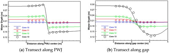
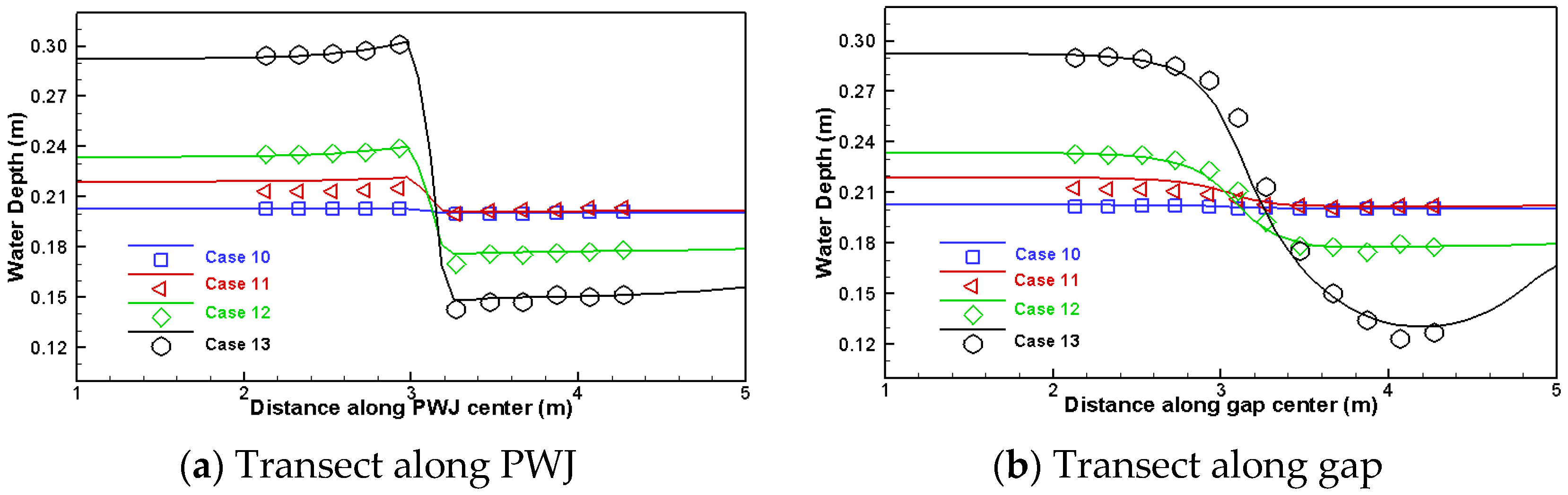
The first set of modeling is carried out to evaluate the predictive capability of the proposed method under varied flow discharge. The set includes cases of 10 to 13—they have the same PWJ (log diameter 0.027 m, porosity 0.6, and blockage 50%) but a range of discharge (0.02 to 0.16 m³/s with the Froude number from 0.07 to 0.57). Using either the low flow of 0.02 m³/s or the high flow of 0.16 m³/s, the LWS coefficient is found to be 0.7 (the backwater rise is used for the calibration).

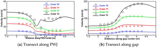
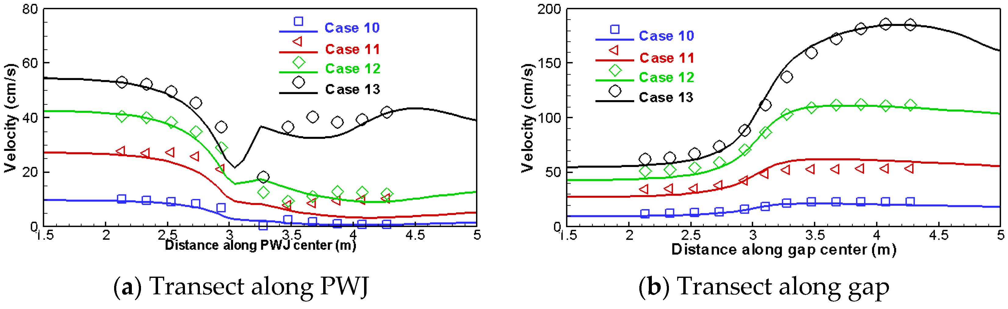
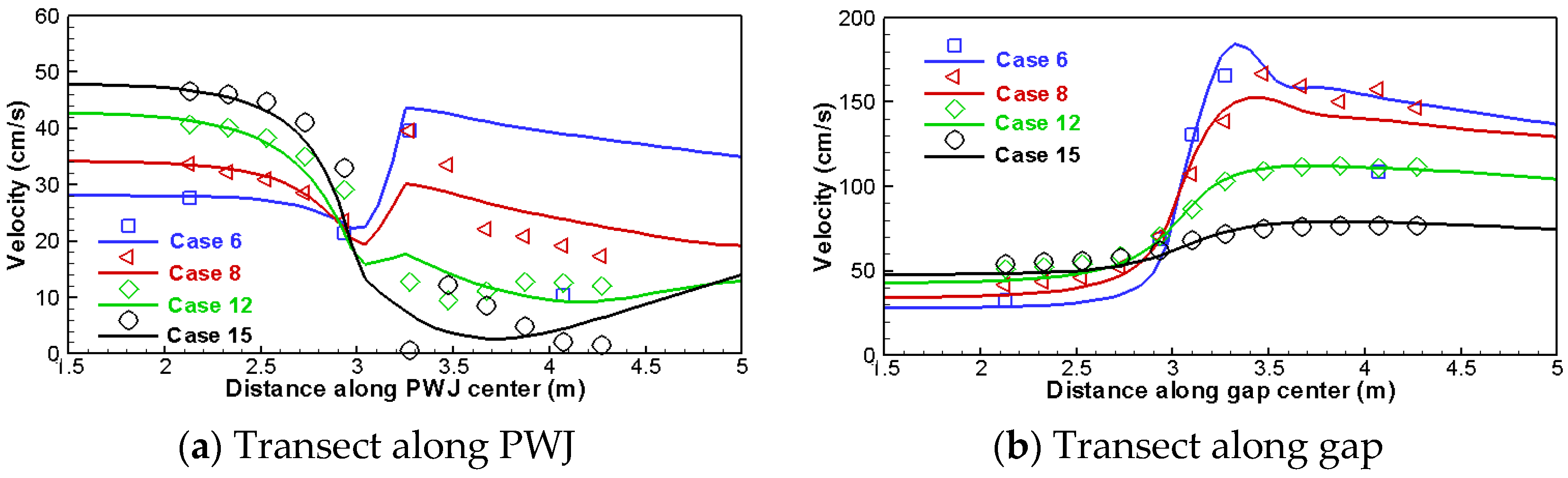
The results are compared in Figure 2 and Figure 3, in which the water depth and velocity are compared along two longitudinal transects (one along the middle of the PWJ and the other along the middle of the gap). The agreement between the prediction and measurement is seen as good. Further, a quantitative comparison is performed by computing the statistical values of the differences between the model and data—all measured points are used along the two measurement transects. Error indicators include the mean error (ME) and root-mean-square errors (RMSEs), and two goodness-of-fit indices are also used, i.e., the Nash–Sutcliffe coefficient (NS coefficient N) and index-of-agreement (I). The NS coefficient determines the relative magnitude of residual variance to the measured data variance. It ranges from negative infinity to 1.0, with N = 1.0 corresponding to a perfect match. The index-of-agreement I is between 0 and 1, with 1 meaning a perfect match. N and I are comparable to the R² index but were found better suited to evaluate the goodness-of-fit according to [47]. These statistical indices are well-known, and a detailed definition is omitted.

Figure 2. Comparison of predicted and measured water depth with cases 10–13.

Figure 3. Comparison of predicted and measured velocity with cases 10–13.

Results of the statistical indices are listed in Table 2; they point to a very good performance by the model. ME is 0.3% of the mean water depth and 2.0% of the mean velocity, while RMSE is 1.7% of the mean water depth and 11% of the mean velocity. Both goodness-of-fit indicators exceed 0.98. The porous-media method is shown capable of predicting flows under different conditions once the LWS coefficient is calibrated using one flow condition—at least for the PWJ dataset studied. More data will be used later to confirm this finding.

Table 2. Statistical error and goodness-of-fit indicators with the partial-spanning PWJ cases.

Case	Variable	ME	RMSE	N	I
10 to 13	Water Depth	−0.55 mm	3.4 mm	0.992	0.998
	Velocity	0.89 cm/s	4.9 cm/s	0.988	0.997
6, 8, 12 & 15	Water Depth	1.56 mm	14.1 mm	0.951	0.986
	Velocity	0.91 cm/s	9.26 cm/s	0.964	0.991

A second dataset is selected to examine the effect of PWJ blockage on model results given the same PWJ packaging (i.e., the same log diameter of 0.027 m and porosity of 0.6). In the literature, it has been reported that blockage is important in impacting the backwater rise. This dataset consists of two subsets: four cases (6, 8, 12 and 15) at a high discharge of 0.1 m³/s (Froude number 0.36) and five cases (1, 4, 7, 10 and 14) at a low discharge of 0.02 m³/s (Froude number 0.07). The blockage value includes 100%, 90%, 75%, 50% and 25%. The same calibrated LWS coefficient of 0.7 is used for all simulations; no recalibration is attempted to obtain a better agreement.

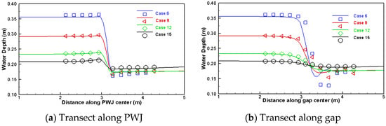
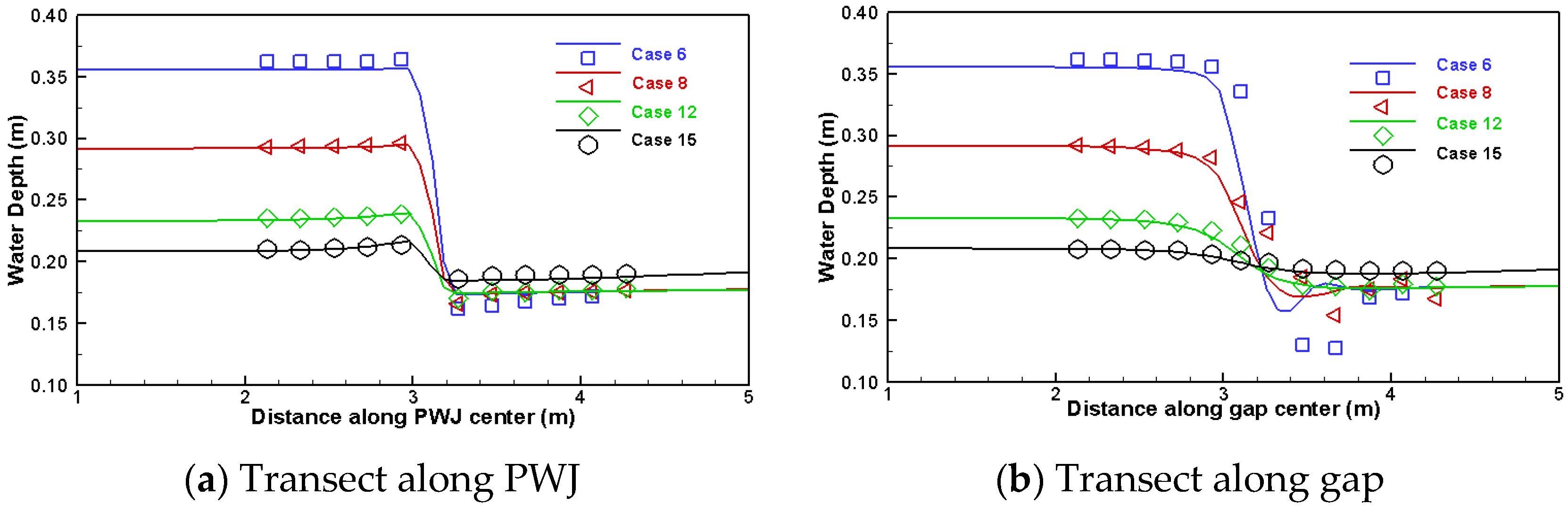
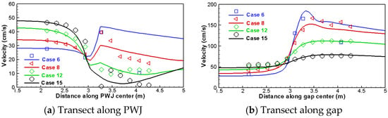
The predicted results are compared with the measured data for the four high-discharge cases in Figure 4 and Figure 5, while the error and goodness-of-fit indicators are listed in Table 2. The low-discharge results produce better agreement but are not shown here—they are included in the comparison later when all cases are presented. It is seen that PWJ blockage has relatively a small effect on the LWS coefficient; therefore, it is not explored further in this study as an independent parameter impacting the LWS coefficient. Again, the agreement between the model and measurement is satisfactory with this set of PWJ data. The major discrepancy is limited to the velocity prediction downstream of the PWJ. Such a discrepancy is expected in view of the highly 3D nature of the flows immediately downstream of the PWJ, which cannot be predicted well by a 2D model, as discussed in [37]. The results suggest that the blockage effect on the LWS coefficient may be unimportant. In practice, it is recommended that no additional calibration be necessary for the blockage effect. Note that this recommendation is based only on a small set of PWJ data and should be regarded as tentative.

Figure 4. Comparison of predicted and measured water depth for cases 6, 8, 12 and 15.

Figure 5. Comparison of predicted and measured velocity with cases 6, 8, 12 and 15.

5.1.3. Effect of Varying Porosity

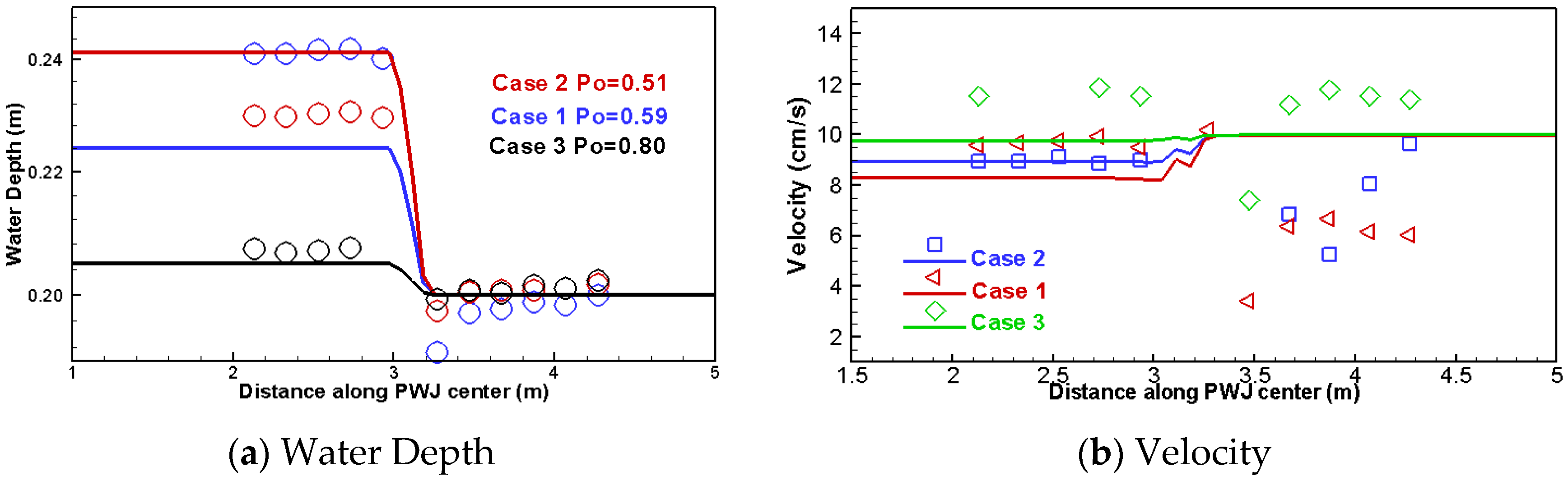
The porosity effect on the LWS coefficient is examined using another set of cases (cases 1 to 3)—these are the only cases available to examine the porosity effect with this dataset. The reported porosity is 0.59, 0.51 and 0.8, respectively. Other properties include 100% blockage and a flow discharge of 0.02 m³/s (Froude number 0.07). The simulation is again carried out using the LWS coefficient of 0.7.

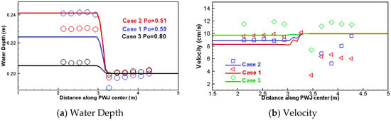
The predicted water depth and velocity along the middle of PWJ are compared with the measured data in Figure 6. It is seen that the predicted results have high errors and deviate from measurement appreciably. It is also noted that the measured water depth for case 1 has a higher backwater rise than case 2, despite case 1 having a smaller porosity. This result seems unlikely and may indicate that other factors are responsible. For this reason, this set of data is deemed insufficient to examine the porosity effect. Despite the issue, however, the results do suggest that PWJ porosity may impact the LWS coefficient, and more investigation is needed. This will be carried out later when the channel-spanning dataset is simulated.

Figure 6. Comparison of water depth and velocity variation for cases 1, 2 and 3.

5.1.4. Results of All Cases

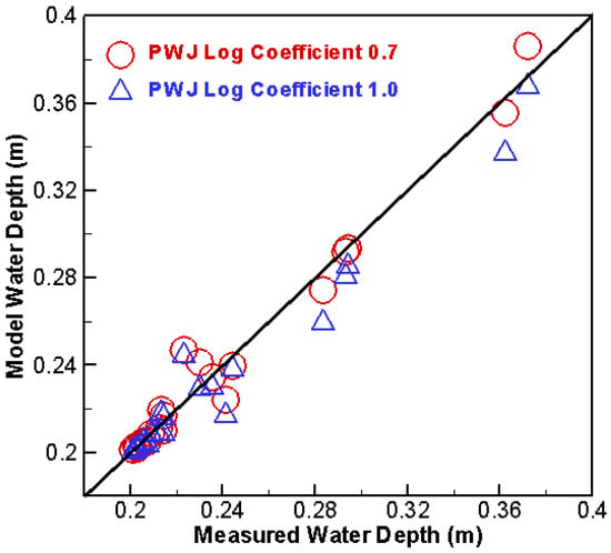
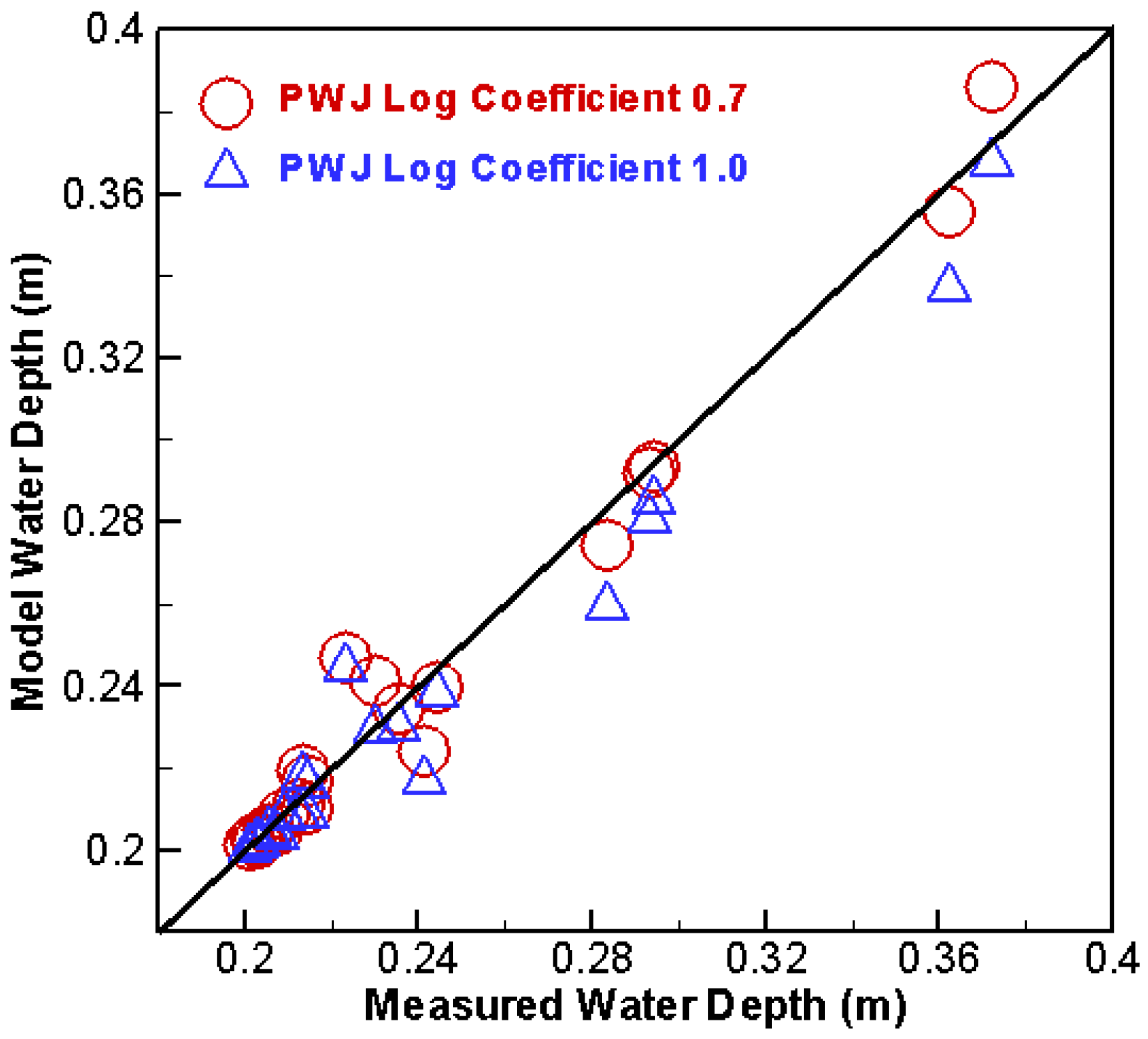
Model results of all 20 cases are obtained by applying the calibrated LWS coefficient of 0.7. The predicted and measured backwater rise (the water depth at the upstream-most measurement point) is compared in Figure 7. In the figure, an additional set of numerical model results is included, computed using simply a unity LWS coefficient (i.e., 1.0). The model is shown to predict well the backwater rise, even though only one calibrated LWS coefficient is applied for all cases (varying flow and blockage). A larger discrepancy is associated with cases that have different porosity—an indication of the dependency of the LWS coefficient on porosity. It is further found that the method of simply applying the unity LWS coefficient also achieves reasonable results—with only 6% underprediction (higher errors are associated with an increased backwater rise). It suggests that the LWS coefficient close to 1.0 may be used when no measured data is available for calibration. These results support the advantage of the proposed method: the LWS log diameter, easily measurable in the field, may be used as the length scale.

Figure 7. Comparison of predicted and measured backwater rise at the upstream-most measurement point for all 20 cases.

5.2. Channel-Spanning PWJs

The porous-media method is evaluated further using the channel-spanning PWJs experimentally studied in [32]. The dataset consisted of more than 200 cases, covering a wide range of PWJ properties (porosity, log diameter and longitudinal length) and flow conditions (discharge and water depth).

5.2.1. The Experiment and Numerical Model

A laboratory study of channel-spanning PWJs was carried out by [25,32]. The series-A dataset had no organic leaves and was used in the present study. The flume was straight—8.0 m long, 0.4 m wide and 0.7 m deep. The inlet section was equipped with two flow straighteners to suppress secondary currents and surface waves so that a uniform flow up to 0.07 m³/s was generated. The flow was controlled at the exit by a sharp-crested weir and generated a stage between 0.05 and 0.15 m. Box-shaped channel-spanning PWJs were placed 3.0 m downstream of the inlet by packing logs between two aluminum racks. PWJs created had a high-enough vertical height that no overtop flows occurred. Schalko et al. [25] found that the aluminum rack had a negligible effect on the approach flow condition and did not induce measurable backwater rise. An illustrative side view of the flume setup is shown in Figure 1.

PWJs were packaged using natural woody logs with various log diameters—see [25,32] for details. Important PWJ properties include (a) average log diameter between 2.3 and 15.0 mm (some used mixed-size logs); (b) porosity between 0.5 and 0.8, covering the dense (0.50–0.67), medium (0.67–0.75) and loose (0.75–0.80) categories according to the classification of Schalko et al. [25]; (c) longitudinal length between 0.05 and 0.2 m; and (d) average log length in the range of 0.05–0.3 m (not explicitly used by the porous-media method).

The flow conditions varied widely—the discharge ranged from 0.003 to 0.056 m³/s and the corresponding Froude number ranged from 0.2 to 1.4. The unobstructed flow depth ($h_0$), taken as the stage at the flume exit, varied between 0.05 and 0.15 m. The flow Reynolds number, based on the approach velocity and hydraulic radius computed by W$h_0$/(W + 2$h_0$) with W being the channel width, was more than 10,000—so the flows were turbulent. The study of [25] estimated the measurement errors: (a) PWJ porosity about ±10%; (b) mean log diameter about ±0.5 mm; and (c) backwater rise up to 15% with an average error of 5%.

The 2D numerical modeling inputs are as follows. The model domain has a total longitudinal length of 7.0 m and lateral width of 0.4 m. The box-shaped PWJ is placed 3.0 m downstream of the inlet and has several longitudinal lengths. The 2D mesh has a total of 2,300 mesh cells with 115 longitudinal cells and 20 lateral cells—much fewer lateral cells are needed for the channel-spanning PWJ than the partial-spanning counterpart, as lateral flow variation is small. Finer longitudinal resolution is used within and near the PWJ, and the average resolution is 0.01 m. The mesh conforms to the recommendation by [37].

Key numerical model inputs are as follows. Flow discharge is imposed as the inlet boundary condition according to each experimental case, while flow stage (water depth)—the reported unobstructed water depth—is imposed as the boundary condition at the exit. The LWS coefficient is the primary input that is to be calibrated with the porous-media method.

5.2.2. Results of All Cases

First, all 262 A-series cases are simulated using the porous-media method. The LWS coefficient is calibrated using one flow for each unique PWJ packaging (i.e., the same values of porosity, log diameter and longitudinal length)—this is to follow the recommended calibration guideline. The calibrated coefficient is then adopted to simulate remaining cases that have different flows (i.e., varied discharge and exit stage). A total of 42 distinct PWJs are identified and simulated. For consistency, the flow case with a Froude number of 0.6, a mid-value of the measured range, is selected for calibration. Schalko et al. [25] identified a dimensionless parameter, named diversion factor (u), as important—it is the ratio of the PWJ’s longitudinal length to the log diameter. The diversion factor was found to be one of the PWJ parameters impacting the backwater rise (the other two are porosity and Froude number). Therefore, the diversion factor is used in this study in place of the PWJ’s longitudinal length from now on in the discussion.

For all PWJs simulated, the calibrated LWS coefficient is found ranging between 0.43 and 2.04. This range may be used as a tentative range in applications. However, it is pointed out that a narrower range between 0.62 and 1.58 is found if four PWJs are excluded. Three of the excluded four, A30, 31 and 39, produced the LWS coefficient above 1.6 and are associated with the smallest log diameter of 2.3 mm (the highest diversion factor). It may suggest that the LWS coefficient is dependent on the diversion factor. The remaining excluded one is the PWJ with A25–26; it leads to the smallest coefficient of 0.43. For this case, however, the backwater rise is significantly overpredicted for the remaining flows—an indication that the measured data may have a high uncertainty. The LWS coefficient would be above 0.6 if any of the other flows were used for calibration. This data point, therefore, is an outlier and should not be included in evaluation.

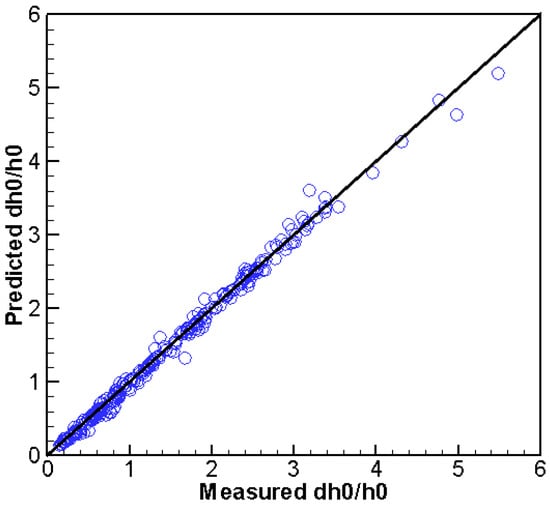
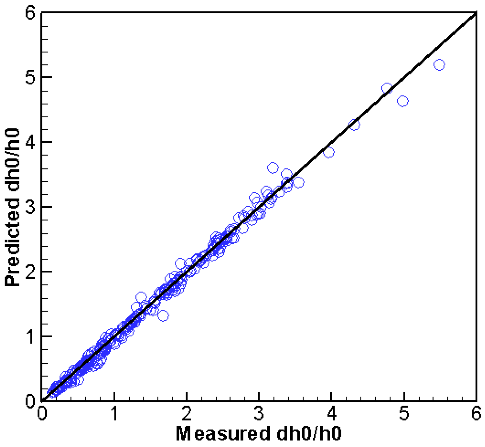
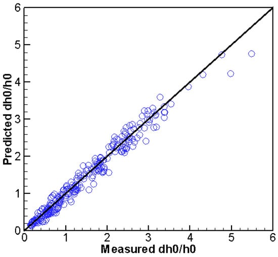
The predicted and measured backwater rise is compared in Figure 8 for all 262 cases comprising 42 PWJs. Overall, the agreement is very good. A statistical error analysis for the entire dataset shows a mean error of the backwater rise of 2.0 mm, an absolute mean error of 4.6 mm, and an RMSE of 14.0 mm—corresponding to 1.6%, 3.7% and 11% of the measured mean. The NS coefficient and index-of-agreement are 0.975 and 0.994, respectively. The quantitative error indices confirm that the model prediction is good by following the suggested general guideline for model calibration—i.e., for each unique PWJ, only one flow is needed for LWS coefficient calibration. Note that the reported error of the measured backwater rise was up to 15% and a mean of 5%, which is comparable to the model prediction errors.

Figure 8. Comparison of predicted and measured $d{h}_0$/$h_0$ for all 262 A-series cases of [32] ($d{h}_0$ is the backwater rise and $h_0$ is the unobstructed water depth).

5.2.3. Effect of PWJ Porosity

It is widely known that PWJ properties impact the resistance force, and one of the most important is porosity. The partial-spanning PWJ results earlier also show that the LWS coefficient may be dependent on the porosity, though it is inconclusive due to the limited number of cases available. With the extensive dataset of [32], the porosity effect can be thoroughly investigated now and discussed next.

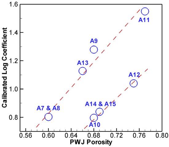
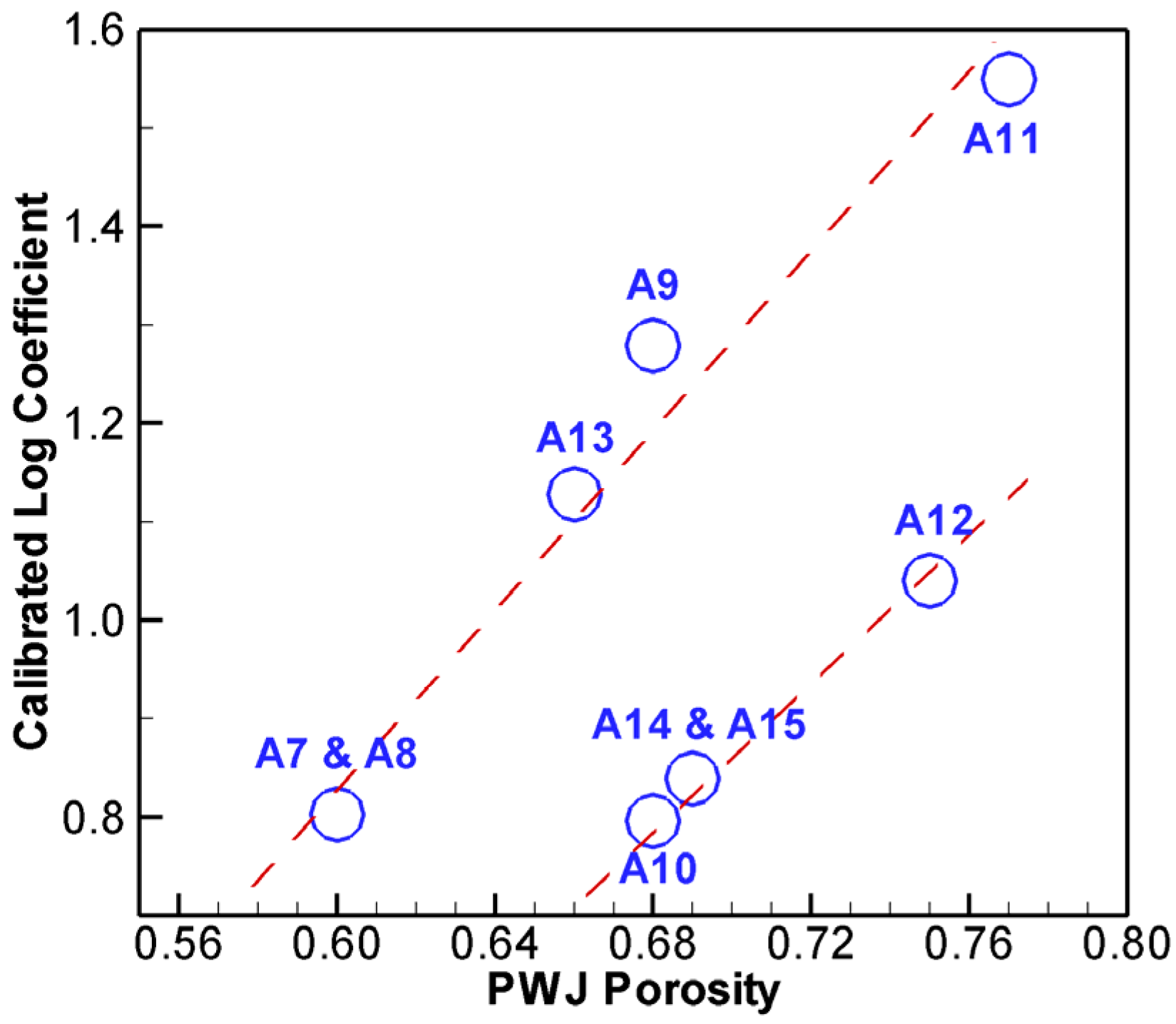
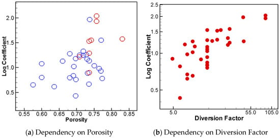
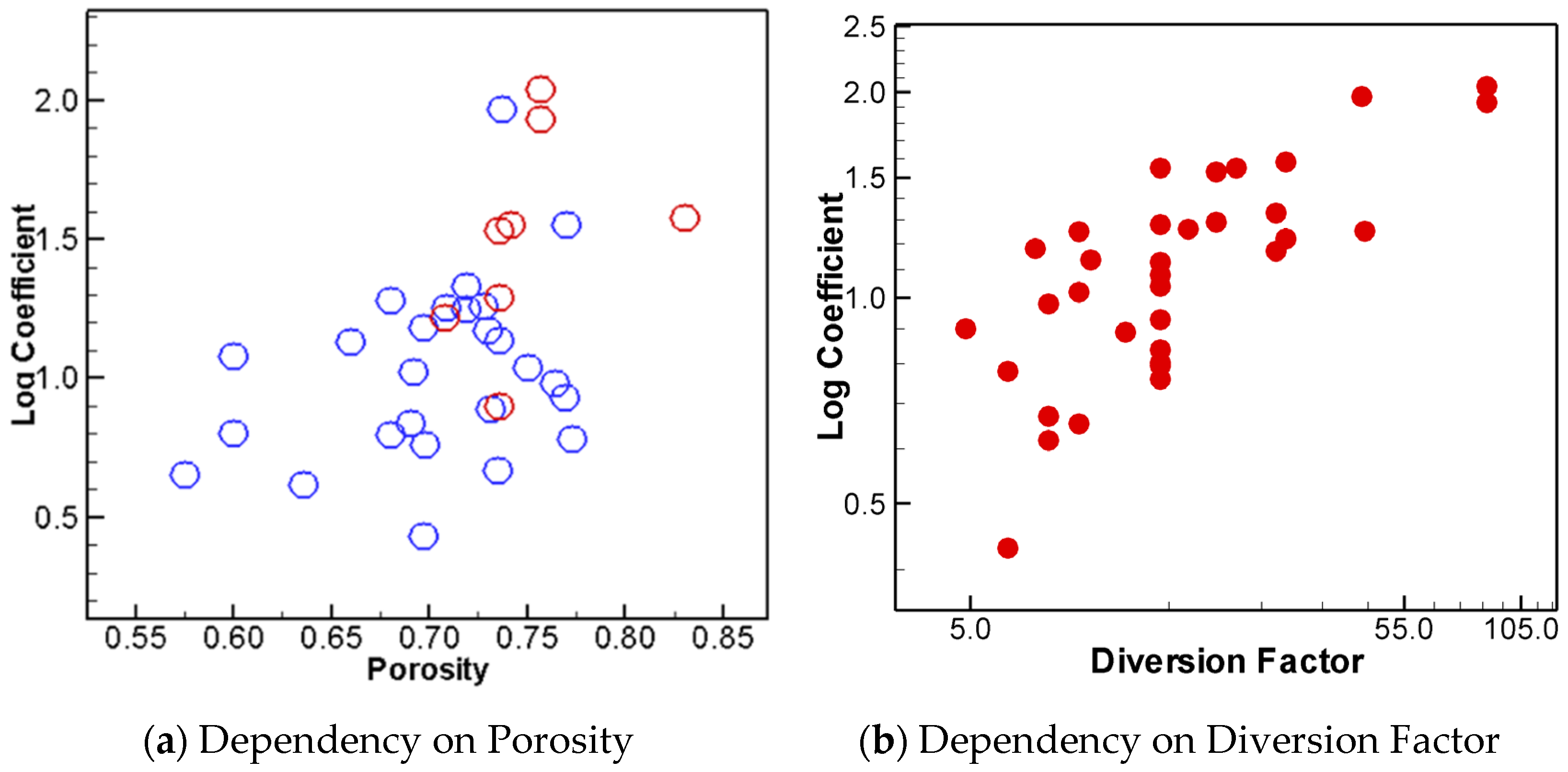
As a first step, 69 cases, series A7–15, are simulated to investigate the porosity effect. This set includes six different porosity values between 0.6 and 0.77; it has the same diversion factor of 14.3 and log diameter of 0.007 m but includes various flows (Froude number from 0.2 to 1.4; water depth from 0.05 to 0.10 m). The calibrated LWS coefficient is shown in Figure 9 against porosity. It is seen that the LWS coefficient is indeed a function of the porosity. There is a general trend of increasing coefficient with increasing porosity. To gain a better understanding, the results of all 262 cases are plotted in Figure 10a. Similar results are obtained, although much more scatter is displayed. If a linear relationship is used for regression, the LWS coefficient may be estimated by ${\alpha }_{Log}=3.39p-1.286$. This linear fit, however, has a low fidelity: the R² coefficient of determination is 0.235 with the correlation coefficient 0.485. The results suggest that porosity alone is insufficient to obtain a reliable estimate. One cause of the scatters may be due to the log surface roughness, such as the presence of barks and/or leftover cut-off branches, but it is not viable to be studied further due to lack of data.

Figure 9. Dependency of log coefficient on porosity based on all cases of A7–A15.

Figure 10. Dependency of log coefficient on porosity and diversion factor: (a) porosity effect with blue symbols from 34 PWJs with a longitudinal length of 0.1 m and red from 8 PWJs with a longitudinal length of 0.05 m and 0.2 m; (b) diversion factor effect.

Another PWJ property, the diversion factor, is explored for its effect on the LWS coefficient, encouraged by the study of [25]. The results of the LWS coefficient and diversion factor are plotted in Figure 10b. The diversion factor is clearly shown to impact the LWS coefficient, and a non-linear relationship exists. It is also shown that the relation between diversion factor and the LWS coefficient has a lesser scatter than porosity. If power regression is applied, the LWS coefficient may be estimated by 0.417$u^{0.35}$. This regression has an R² coefficient of determination of 0.6 and a correlation coefficient of 0.77—a much better equation than relying on the porosity alone.

5.2.4. A Regression Equation

The above results show that the LWS coefficient is a function of both porosity and diversion factor. Additional uncertainty, if it exists, may be attributed to factors such as the log surface roughness (not explored herein due to lack of data). In the following, a regression equation is developed to estimate the LWS coefficient using both porosity and diversion factor. Note that porosity and diversion factor may be easily estimated in the field, and such a regression can be useful in practical applications when no measured data is available for the recommended calibration.

After trials of several functional forms, a relatively simple power model, in the form of $a{X}_1^b{X}_2^c$, is adopted. The recommended regression equation is expressed as follows:

$${\alpha }_L=0.815p^{1.56}{u}^{0.3}$$

(5)

The above regression has an R² coefficient of determination of 0.7 and a correlation coefficient of 0.84. This equation is recommended for use to estimate the LWS coefficient when no measured backwater rise data is available for calibration. This regression is only needed to estimate the PWJ porosity, mean log diameter and longitudinal length.

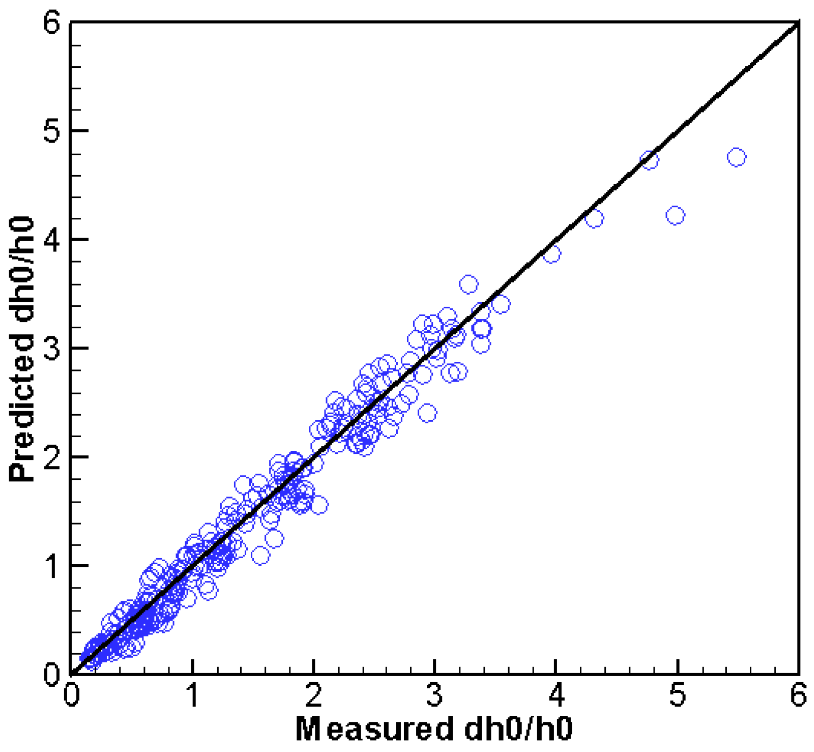
The above regression equation is evaluated for its performance: all 262 cases are re-simulated by using the LWS coefficient computed solely by the regression equation. The predicted backwater rise is compared with the measured data in Figure 11. A visual inspection shows that the results, as expected, have a larger scatter than those calibrated (see Figure 8) but are satisfactory. The statistical error analysis shows that the mean error of the backwater rise is 3.1 mm, the absolute mean error is 11.8 mm, and the RMSE is 19 mm, which corresponds to 2.5%, 9.5% and 15.3% of the measured means. The NS coefficient and index-of-agreement are 0.954 and 0.989, respectively. The quantitative error results confirm that the prediction using the regression is still satisfactory with the porous-media method, considering that the reported mean error of the measured rise was 5% (up to 15% is possible). Note that the error range of the present method performed better than the mixed method of Altmann et al. [36], who used the same dataset for modeling. The Altmann method predicted the backwater rise within 30% of the prediction range.

Figure 11. Comparison of predicted and measured $d{h}_0/h_0$ for all 262 A-series cases of [32] when the log coefficient is computed from the regression equation only.

Limitations of the regression equation need to be kept in mind: it is probably limited to the channel-spanning PWJs and may be additionally limited to the parameter ranges of the data used to obtain the regression—i.e., porosity between 0.5 and 0.8 and diversion factor between 4.8 and 87. Future verification is needed for its applicability to other ELJ types and in the field.

6. Conclusions

A porous-media method is adapted and extended from groundwater flow models to simulate stream flows with the LWS’s presence. The method computes the LWS resistance force using a combined linear Darcy term and quadratic Forchheimer term. Only one calibration parameter, called the LWS coefficient, is proposed with the present method. The method is evaluated using two sets of laboratory data—the partial-spanning PWJ data of Schalko et al. [33] and the channel-spanning data of Schalko [32]. Major conclusions are summarized below.

A general guideline is developed in applying the proposed porous-media method; it consists of the following procedure: (1) The LWS coefficient should first be calibrated for each unique LWS using measured data under at least one flow condition; the upstream backwater rise may be used to perform the calibration. (2) If there are no measured data for calibration, the empirical equation developed in this study may be used to provide an estimate of the coefficient, but its validity remains to be verified beyond PWJs. (3) The obtained LWS coefficient can then be used to simulate different or unsteady flows as far as the LWS remains the same.

The proposed porous-media method is found to predict the flows well, using two sets of laboratory data with PWJ presence, when the proposed guideline is followed. The differences between the model prediction and measured data are small and mostly within the measurement errors. The proposed porous-media method can potentially be a viable tool in practical applications, as the general guideline may be readily followed by engineers (measured data under one flow condition is often available).

An advantage of the proposed porous-media method is that the LWS coefficient has a clear physical meaning: it is the ratio of the log size to the LWS log diameter, which is easily estimated in the field, and the log size is close to the log diameter. Indeed, the coefficient is found within a relatively narrow range with the PWJ datasets studied—e.g., between 0.6 and 1.6.

A tentative regression equation is also developed to estimate the LWS coefficient according to the PWJ type. Such a regression can be useful in practical applications when no measured data is available for model calibration. The computed backwater rise using the regression equation is found to satisfactorily agree with the measured PWJ data—the differences are found close to the reported measurement errors, and it performed better than the method in [36].

Despite the success of the present method, potential limitations need to be pointed out; they include: (a) the general guideline is yet to be verified using field cases and beyond the PWJ type; (b) good predictions also need to be confirmed with more measured data, in particular, the field data; and (c) the regression equation to estimate the LWS coefficient should be viewed as tentative; its validity may be limited to the parameter ranges of the data used—that is, the LWS type (PWJ only), porosity (0.5 to 0.8), and diversion factor (4.8 to 87). Further, it is cautioned in practical applications that the 2D method is more suitable for far-field results of water level and velocity distribution, as well as for flood inundation extent in river channels; it is not recommended for near-field (e.g., within LWSs) results, which should be simulated using high-resolution 3D CFD models.

Future work includes two areas. One is the simulation of other LWS types such as ELJs; another is to perform more verifications to confirm the findings of this study. In particular, field data is needed to verify the general guideline and application procedure. The finding that the LWS coefficient is not a function of the flow conditions also needs to be verified in the field.

References

- Bennett, S.J.; Ghaneeizad, S.M.; Gallisdorfer, M.S.; Cai, D.; Atkinson, J.F.; Simon, A.; Langendoen, E.J. Flow, turbulence, and drag associated with engineered log jams in a fixed-bed experimental channel. Geomorphology 2015, 248, 172–184. [Google Scholar] [CrossRef] [Scilit]
- Beechie, T.J.; Sear, D.A.; Olden, J.D.; Pess, G.R.; Buffington, J.M.; Moir, J.; Roni, P.; Pollock, M.M. Process-based principles for restoring river ecosystems. BioScience 2010, 60, 209–222. [Google Scholar] [CrossRef] [Scilit]
- USBR (Bureau of Reclamation); ERDC (U.S. Army Engineer Research and Development Center). National Large Wood Manual: Assessment, Planning, Design, and Maintenance of Large Wood in Fluvial Ecosystems: Restoring Process, Function, and Structure. 2016. Available online: https://ewn.erdc.dren.mil/wp-content/uploads/2021/03/National_Large_Wood_Manual-USBR_USACE-January2016-FINAL2.pdf (accessed on 15 February 2026).
- Jeffries, R.; Darby, S.E.; Sear, D.A. The influence of vegetation and organic debris on flood-plain sediment dynamics: Case study of a low-order stream in the New Forest, England. Geomorphology 2003, 51, 61–80. [Google Scholar] [CrossRef] [Scilit]
- Abbe, T.B.; Brooks, A.; Montgomery, D.R. Wood in River Rehabilitation and Management. In The Ecology and Management of Wood in World Rivers; Gregory, S., Brurnell, K., Boyer, A., Eds.; American Fisheries Society: Bethesda, MD, USA, 2003; pp. 367–391. [Google Scholar]
- Le Lay, Y.-F.; Piegay, H.; Moulin, B. Wood Entrance, Deposition, Transfer and Effects on Fluvial Forms and Processes: Problem Statements and Challenging Issues. In Treatise on Geomorphology; Shroder, J.F., Butler, D.R., Hupp, C.R., Eds.; Academic Press: San Diego, CA, USA, 2013; pp. 20–36. [Google Scholar]
- Comins, L.; Garft, D.; Spray, C.; MacDonald, A. Eddleston Water Project Report, 2016. Available online: https://ewn.erdc.dren.mil/wp-content/uploads/2021/03/case_study_9_eddleston.pdf (accessed on 27 March 2026).
- Shields, F.D.; Knight, S.S.; Stofleth, J.M. Large wood addition for aquatic habitat rehabilitation in an incised, sand-bed stream, little Topashaw Creek, Mississippi. River Res. Appl. 2006, 22, 803–817. [Google Scholar] [CrossRef] [Scilit]
- Addy, S.; Wilkinson, M.E. An assessment of engineered log jam structures in response to a flood event in an upland gravel-bed river. Earth Surf. Process. Landf. 2016, 41, 158–1670. [Google Scholar] [CrossRef] [Scilit]
- Abbe, T.B.; Brooks, A. Geomorphic, Engineering, and Ecological Considerations When Using Wood in River Restoration. In Stream Restoration in Dynamic Fluvial Systems: Scientific Approaches, Analyses, and Tools; Simon, A., Bennett, S., Castro, J., Eds.; American Geophysical Union: Washington, DC, USA, 2011; pp. 419–451. [Google Scholar]
- Polvi, L.E.; Wohl, E. Biotic drivers of stream planform: Implications for understanding the past and restoring the future. BioScience 2013, 63, 439–452. [Google Scholar] [CrossRef] [Scilit]
- Allen, J.B.; Smith, D.L. Characterizing the impact of geometric simplification on large woody debris using CFD. Int. J. Hydraul. Eng. 2012, 1, 1–14. [Google Scholar] [CrossRef]
- Lester, R.E.; Boulton, A.J. Rehabilitating agricultural streams in Australia with wood: A review. Environ. Manag. 2008, 42, 310–326. [Google Scholar] [CrossRef] [Scilit] [PubMed]
- Roni, P.; Beechie, T.; Pess, G.; Hanson, K. Wood placement in river restoration: Fact, fiction, and future direction. Can. J. Fish. Aquat. Sci. 2014, 72, 466–478. [Google Scholar] [CrossRef] [Scilit]
- Lautz, L.K.; Siegel, D.I.; Bauer, R.L. Impact of debris dams on hyporheic interaction along a semi-arid stream. Hydrol. Process. 2006, 20, 183–196. [Google Scholar] [CrossRef] [Scilit]
- Flores, L.; Larranaga, A.; Diez, J.; Elosegi, A. Experimental wood addition in streams: Effects on organic matter storage and breakdown. Freshw. Biol. 2011, 56, 2156–2167. [Google Scholar] [CrossRef] [Scilit]
- Xu, Y.; Liu, X. Effects of different in-stream structure representations in computational fluid dynamics models—Taking engineered log jams (ELJ) as an example. Water 2017, 9, 110. [Google Scholar] [CrossRef] [Scilit]
- Kimura, I.; Kitazono, K. Effects of the driftwood Richardson number and applicability of a 3D-2D model to heavy wood jamming around obstacles. Environ. Fluid Mech. 2020, 20, 503–525. [Google Scholar] [CrossRef] [Scilit]
- Lai, Y.G.; Smith, D.L.; Bandrowski, D.J.; Xu, Y.; Woodley, C.M.; Schnell, K. Development of a CFD model and procedure for flows through in-stream structures. J. Appl. Water Eng. Res. 2021, 10, 197–211. [Google Scholar] [CrossRef] [Scilit]
- Ruiz-Villanueva, V.; Blade, E.; Sanchez-Juny, M.; Marti-Cardona, B.; Dıez-Herrero, A.; Bodoque, J.M. Two-dimensional numerical modeling of wood transport. J. Hydroinformatics 2014, 16, 1077–1096. [Google Scholar] [CrossRef] [Scilit]
- Persi, E.; Petaccia, G.; Sibilla, S. Large wood transport modelling by a coupled Eulerian-Lagrangian approach. Nat. Hazards 2017, 91, 59–74. [Google Scholar] [CrossRef] [Scilit]
- Sixta, M.; Ubing, C. Representation of Large Wood Structures Using a Numerical Two-Dimensional Model. Final Report ST-2019-1756-01, Research and Development Office, Science and Technology Program, U.S. Bureau of Reclamation, Denver, Colorado. 2019. Available online: https://www.usbr.gov/research/projects/researcher.cfm?id=2211 (accessed on 15 May 2022).
- Manners, R.B.; Doyle, M.W.; Small, M.J. Structure and hydraulics of natural woody debris jams. Water Resour. Res. 2007, 43, W06432. [Google Scholar] [CrossRef] [Scilit]
- Tullos, D.; Walter, C. Fish use of turbulence around wood in winter: Physical experiments on hydraulic variability and habitat selection by juvenile coho salmon, oncorhynchus kisutch. Environ. Biol. Fishes 2015, 98, 1339–1353. [Google Scholar] [CrossRef] [Scilit]
- Schalko, I.; Schmocker, L.; Weitbrecht, V.; Boes, R.M. Backwater rise due to large wood accumulations. J. Hydraul. Eng. 2018, 140, 04018056. [Google Scholar] [CrossRef] [Scilit]
- Ventres-Pake, R.; Nahorniak, M.; Kramer, N.; O’Neal, J.; Abbe, T. Integrating large wood jams into hydraulic models: Evaluating a porous plate modeling method. J. Am. Water Resour. Assoc. 2020, 56, 333–347. [Google Scholar] [CrossRef] [Scilit]
- Nahorniak, M.; Wheaton, J.; Volk, C.; Bailey, P.; Reimer, M.; Wall, E.; Whitehead, K.; Jordan, C. How do we efficiently generate high-resolution hydraulic models at large numbers of riverine reaches? Comput. Geosci. 2018, 119, 80–91. [Google Scholar] [CrossRef] [Scilit]
- Addy, S.; Wilkinson, M.E. Representing natural and artificial in-channel large wood in numerical hydraulic and hydrological models. WIREs Water 2019, 6, e1389. [Google Scholar] [CrossRef] [Scilit]
- Nisbet, T.; Silgram, M.; Shah, N.; Morrow, K.; Broadmeadow, S. Woodland for Water: Woodland Measures for Meeting Water Framework Directive Objectives. Surrey: Retrieved from Forest Research. 2011. Available online: https://www.ecrr.org/Portals/27/scho0711btyr-e-e.pdf (accessed on 27 March 2026).
- Metcalfe, P.; Beven, K.; Hankin, B.; Lamb, R. A modelling framework for evaluation of the hydrological impacts of nature-based approaches to flood risk management, with application to in-channel interventions across a 29-km2 scale catchment in the United Kingdom. Hydrol. Process. 2017, 31, 1734–1748. [Google Scholar] [CrossRef] [Scilit]
- Pinto, C.; Ing, R.; Browning, B.; Delboni, V.; Wilson, H.; Martyn, D.; Harvey, G.L. Hydromorphological, hydraulic and ecological effects of restored wood: Findings and reflections from an academic partnership approach. Water Environ. J. 2019, 33, 353–365. [Google Scholar] [CrossRef] [Scilit]
- Schalko, I. Modeling Hazards Related to Large Wood in Rivers, VAW-Mitteilungen 249, Versuchsanstalt für Wasserbau, Hydrologie und Glaziologie (VAW); Boes, R.M., Ed.; ETH: Zürich, Switzerland, 2018; Available online: https://www.ethz.ch/content/dam/ethz/special-interest/baug/vaw/vaw-dam/documents/das-institut/mitteilungen/2010-2019/249.pdf (accessed on 20 November 2021).
- Schalko, I.; Follett, E.; Nepf, H. Impact of lateral gap on flow distribution, backwater rise, and turbulence generated by a logjam. Water Resour. Res. 2023, 59, e2023WR034689. [Google Scholar] [CrossRef] [Scilit]
- Schalko, I. Dataset: Backwater Rise Due to Large Wood Accumulations. 2018. Available online: https://zenodo.org/record/2640932 (accessed on 20 November 2021).
- Schalko, I. Dataset: Impact of Lateral Gap on Flow Distribution, Backwater Rise, and Turbulence Generated by a Logjam. 2023. Available online: https://zenodo.org/records/8415089 (accessed on 10 October 2023).
- Altmann, M.; Vanzo, D.; Valero, D.; Schalko, I. A simple approach to simulate logjams in two-dimensional hydrodynamic models. J. Hydraul. Eng. 2024, 150, 06024002. [Google Scholar] [CrossRef] [Scilit]
- Radiyan, F.M.; Liu, X. Flow Partition in Two-Dimensional Open Channels with Porous Structures. Sci. Rep. 2025, 15, 28255. [Google Scholar] [CrossRef] [Scilit] [PubMed]
- Lai, Y.G. Two-dimensional depth-averaged flow modeling with an unstructured hybrid mesh. J. Hydraul Eng. 2010, 136, 12–23. [Google Scholar] [CrossRef] [Scilit]
- Tsakiris, A.; Mozes, K.; George, M. Approaches for Simulating Large Woody Material (LWM) in Two-Dimensional (2D) Models. In Proceedings of the National Hydraulic Engineering Conference, Atlanta, Georgia, 16–19 August 2022; Available online: https://www.youtube.com/watch?v=5LUxT_RMphA&list=PL_AexyHkNDwQzO4O3c_I7-Qm2SqtYpuov&index=36 (accessed on 2 October 2025).
- Brooks, A.P.; Abbe, T.B.; Jansen, J.; Taylor, M.; Gippel, C.J. Putting the wood back into our rivers: An experiment in river rehabilitation. In Proceedings of the Third Australian Stream Management Conference: The Value of Healthy Streams; Rutherford, I., Sheldon, F., Brierley, G., Eds.; Cooperative Research Centre for Catchment Hydrology: Clayton, Australia, 2001; pp. 73–80. [Google Scholar]
- Abbe, T.B. Conceptual Design Guidelines: Application of Engineered Logjams. Retrieved from Commissioned Report for SEPA; Scottish Environment Protection Agency: Seattle, WA, USA, 2006. [Google Scholar]
- Pasternack, G.B. 2D Modeling and Ecohydraulic Analysis; University of California at Davis: Davis, CA, USA, 2011. [Google Scholar]
- Wilcox, A.C.; Wohl, E.E. Flow resistance dynamics in step-pool stream channels: Large Woody Debris and Controls on Total Resistance. Water Resour. Res. 2006, 42, 1–14. [Google Scholar] [CrossRef] [Scilit]
- Turcotte, B.; Millar, R.G.; Hassan, M.A. Drag forces on large cylinders. River Res. Appl. 2015, 32, 411–417. [Google Scholar] [CrossRef] [Scilit]
- Van Gent, M.R.A. Wave Interaction with Permeable Coastal Structures. Technical Report Diss 2689. Ph.D. Thesis, Delft University of Technology, Delft, The Netherlands, 1995. Available online: https://www.researchgate.net/publication/27344718 (accessed on 6 October 2024).
- Jensen, B.; Jacobsen, N.G.G.; Christensen, E.D. Investigations on the porous media equations and resistance coefficients for coastal structures. Coast. Eng. 2014, 84, 56–72. [Google Scholar] [CrossRef] [Scilit]
- Legates, D.R.; McCabe, G., Jr. Evaluating the use of “goodness-of-fit” measures in hydrologic and hydroclimatic model validation. Water Resour. Res. 1999, 35, 233–241. [Google Scholar] [CrossRef] [Scilit]
Disclaimer/Publisher’s Note: The statements, opinions and data contained in all publications are solely those of the individual author(s) and contributor(s) and not of MDPI and/or the editor(s). MDPI and/or the editor(s) disclaim responsibility for any injury to people or property resulting from any ideas, methods, instructions or products referred to in the content. |
© 2026 by the author. Licensee MDPI, Basel, Switzerland. This article is an open access article distributed under the terms and conditions of the Creative Commons Attribution (CC BY) license.