


Abstract
Against the backdrop of ongoing climate change, the Qinghai–Tibet Plateau, a region highly sensitive to climatic variation, exhibits intricate spatiotemporal patterns in reference crop evapotranspiration (ETO), with significant implications for regional water-resource planning. This study selected four agro-climatic zones across the plateau region (TSA, TSH, TAZ, and WCH). Long-term daily observations from 28 meteorological stations were used to estimate ETO via the FAO 56 Penman–Monteith equation. This extensive dataset enabled robust trend analysis using the Mann–Kendall test, alongside a cloud-model framework, and analyses of sensitivity and contributions to evaluate ETO’s spatiotemporal evolution, its distributional uncertainty, and the underlying drivers. Results reveal pronounced regional heterogeneity in the interannual variability of ETO. Annual ETO declined in TSH and TSA (trend rates of −1.12 and −6.58 mm·10a−1, respectively) and increased in TAZ and WCH (15.76 and 10.74 mm·10a−1, respectively). At monthly and seasonal timescales, ETO exhibited an unimodal pattern, with the greatest stability in winter and spring and lower stability in summer and autumn. The cloud-model parameter He indicates that ETO stability is greatest in TSH and weakest in WCH, with He values of 7.15 and 12.29 mm, respectively. Contribution-rate analyses identify Tmax and Tmean as the principal determinants of rising ETO across all study zones, reflecting the largest individual contributions. Temperature-related factors together account for the majority of ETO variability across the regions, with their absolute contributions ranging from 5.61% to 8.63%, well above those of aerodynamic factors (0.62–1.78%). Stability assessments indicate that ETO is generally more unstable than its meteorological drivers, with substantial regional disparities, implying that ETO evolution cannot be explained by a single controlling factor. Overall, the study characterizes the uncertainty in ETO variations under complex terrain, highlights the value of the cloud model for refined hydrological assessments, and provides a scientific basis for adaptive agricultural water-resource management in the region.
1. Introduction
Against the backdrop of climate change, reference crop evapotranspiration (ETO) serves as a key indicator of atmospheric evaporative demand and crop-water requirements. It underpins regional water resources planning, guides precision irrigation management, supports drought monitoring, and informs assessments of ecosystem responses under evolving climatic conditions [1,2,3]. Under ongoing climate change, fluctuations in meteorological variables—such as air temperature, solar radiation, wind speed, and humidity—drive the spatiotemporal variability of ETO, posing substantial challenges to the balance between regional water supply and demand and to agricultural production security. Consequently, accurate estimation of ETO and elucidation of its variation patterns and driving mechanisms are essential for developing sustainable water-resource management strategies and for improving irrigation management. Xizang lies at the ecological core and represents a sensitive frontier of the Qinghai–Tibet Plateau. The region features distinctive topography, high-altitude conditions, and fragile ecosystems [4,5], which render it particularly vulnerable to climate change. Therefore, an in-depth investigation of ETO dynamics and their underlying drivers in Xizang has significant scientific and practical significance for quantifying agricultural water demand, informing sustainable water-resource utilization strategies, and optimizing irrigation management [6,7].
Recently, scholars from both domestic and international contexts have conducted extensive research on the variability of ETO and its driving mechanisms. Methodologically, a range of techniques has been used to detect long-term trends in ETO, including the Mann–Kendall trend test [8,9], linear trend analysis [10], and cumulative departure methods [11]. Additionally, methods such as partial correlation analysis [12], sensitivity analyses [13], and contribution-rate analyses [8,14] have been used to examine the contributions of meteorological factors to ETO variation and the underlying mechanisms. These approaches, widely applied across regions, have effectively revealed the spatiotemporal evolution of ETO and its response to climate change [8,15]. Global syntheses indicate that ETO displays complex spatiotemporal variability across recent decades [16,17,18], with declines in some regions and increases in others. This variability closely tracks changes in meteorological factors, including net radiation, wind speed, air temperature, and relative humidity. In the Qinghai–Tibet Plateau, several studies have noted that [19,20,21,22], under rising temperatures and increased solar radiation, ETO has generally risen; however, localized areas have declined or shown no significant change due to wind speed, relative humidity, and other factors. For instance, Tang et al. [8], based on data from 31 meteorological stations on the Tibetan Plateau, found that, with the exception of some Shigatse regions, most of Tibet exhibited an increasing ETO trend directly related to changes in temperature and humidity. Furthermore, under climate warming, agricultural irrigation water demand in Tibet is projected to rise. Liu et al. [19], focusing on three major irrigation districts in Tibet, observed substantial differences in the spatiotemporal distribution patterns of ETO. They identified average wind speed and relative humidity as key influencing factors and documented the existence of the “evaporation paradox” within the irrigation districts [23]. Additionally, machine-learning models, including support vector machines, artificial neural networks, random forests, and multilayer perceptrons, have demonstrated substantial potential in estimating ETO and unveiling nonlinear relationships between meteorological factors and ETO [24,25]. However, these models are frequently described as “black boxes” offering only limited insight into how their internal processes operate [26]. Moreover, their reliance on large training data sets creates obstacles to applying them in the Xizang region [27,28].
In summary, existing analytical approaches have proven effective in characterizing ETO variation across multiple spatiotemporal scales and in identifying the primary meteorological drivers. Nevertheless, many investigations indicate that ETO time series possess intrinsic randomness and ambiguity [29,30], causing traditional statistical approaches to fall short in quantifying uncertainty properties like distributional uniformity and stability within ETO dynamics. A quantitative assessment of ETO uncertainty is essential for clarifying its spatiotemporal variability and the mechanisms driving it, and it provides a methodological basis for advancing ETO theory and enhancing predictive accuracy. The cloud model, originally proposed by academician Deyi Li, provides a powerful framework for bridging qualitative concepts and quantitative representations and explicitly accommodates the coexistence of randomness and fuzziness in natural systems. Within this framework, the expectation (Ex), entropy (En), and hyper-entropy (He) characterize the central tendency, uniformity, and stability of a sequence [31]. Moreover, cloud diagrams facilitate intuitive visualization of distributional uniformity and structural stability [32]. Compared with traditional trend-based approaches, the cloud model provides a more refined quantitative description of attributes such as variation uniformity, fluctuation stability, and the evolution of distributional structure [33]. Accordingly, Bai et al. [34], Zhang et al. [35], Yang et al. [36], Sun et al. [37], and Liu et al. [19] have successfully applied the cloud model in climatological, hydrological, and agricultural studies, achieving significant advances. Notably, Liu et al. [19] were the first to introduce the cloud model to evaluate the temporal uniformity and stability of ETO at the irrigation-district scale in Xizang. These findings provide a methodological basis for extending the cloud model to broader spatial scales in the present study.
Although considerable progress has been made in understanding the patterns of ETO variation and its driving mechanisms on the Xizang Plateau, several limitations persist. Firstly, the majority of studies analyze either the plateau in its entirety or individual river basins [38], leaving insufficient attention to systematic, fine-scale comparisons across diverse agro-climatic zones. Consequently, the heterogeneity of ETO dynamics and of its dominant controlling factors under complex climatic gradients and diverse cropping systems remains inadequately characterized, underscoring the need for targeted comparative analyses. Second, the majority of prior studies rely on deterministic modeling frameworks [20,21], whereas the uncertainty characteristics inherent in ETO variability have received relatively little attention. This omission constrains a comprehensive understanding of the stochastic and structural features shaping ETO evolution. Third, although fluctuations and stability of ETO are likely influenced by the stability of its driving meteorological factors, empirical investigations into this relationship remain scarce. This information gap constrains a deeper understanding of regional water-resource dynamics and hampers the development of adaptive irrigation management strategies within Xizang’s farming systems. Closing these gaps is essential to advance both the theoretical framework and the practical applications of ETO research in high-altitude, climate-sensitive regions. Consequently, this study postulates the following core hypothesis:
We hypothesize that the temporal stability of ETO in the Tibetan Plateau is generally lower than that of its primary meteorological driving factors; furthermore, the coupling relationship between ETO and the stability of its driving meteorological factors is not a simple linear one; instead, it exhibits substantial regional heterogeneity, with its intricate nature being non-linearly modulated by the local climatic context and the synergistic effects of multiple influencing factors.
To address these identified limitations and rigorously test the proposed hypothesis, this study focuses on four representative agro-climatic zones in Xizang—the plateau temperate semi-arid zone, the semi-humid zone, the arid zone, and the cool temperate semi-humid zone—and systematically applies cloud-model theory to examine the multi-temporal variability of ETO and its driving mechanisms. The principal contribution is a pioneering exploration: the first attempt to elucidate the coupling between the temporal stability of ETO and the stability of its dominant meteorological drivers. By applying this analytical framework, we refine our understanding of the processes that govern ETO evolution and of the primary sources of uncertainty across the Xizang Plateau. These findings will thus provide a robust scientific basis for climate-change adaptation in Xizang agriculture, thereby supporting more efficient water-resource allocation and promoting sustainable agricultural development.
2. Materials and Methods
2.1. Overview of the Study Area
The study area covers the central Qinghai–Tibet Plateau within the Tibet Autonomous Region (see Figure 1). The terrain is complex and heterogeneous, with average elevations exceeding 4000 m. The region exhibits typical plateau climate characteristics, including strong solar irradiance and large diurnal temperature ranges, and marked spatial variability in hydrothermal conditions [39]. Annual precipitation is unevenly distributed and follows a distinct wet–dry seasonal pattern: May–September constitutes the wet season, while October through April of the following year constitutes the dry season. Owing to constraints imposed by terrain, topography, and water resources, cultivated land in Xizang is scarce, occurring mainly in belts or patches within valleys and basins [40].
Figure 1.
Topographic features and spatial distribution of meteorological stations in the Xizang Autonomous Region. Elevations derived from a digital elevation model (DEM) range from 24 m to 8746 m above mean sea level (m a.s.l.). Solid black circles (●) indicate meteorological stations located in agricultural zones, whereas red triangles (▲) denote stations in non-agricultural zones.
To systematically elucidate the spatiotemporal evolution of ETO under varying climatic gradients, the study area was subdivided into four agro-climatic zones following the established agricultural climatic regionalization framework [41,42]: TSA (plateau temperate semi-arid), TSH (plateau temperate semi-humid), TAZ (plateau temperate arid), and WCH (plateau warm–cool temperate semi-humid). These zones exhibit marked variations in hydrothermal conditions and, together, encompass Xizang’s major agricultural production systems and key farming areas, thereby ensuring the representativeness and coherence of the analytical framework.
2.2. FAO 56 Penman–Monteith Model
The FAO 56 Penman–Monteith method is widely regarded as the standard approach for estimating ETO because of its physical basis and accuracy [43]. In accordance with Allen et al. [44], the equation used in this study is shown below:
In the equation, the following apply:
- : reference crop evapotranspiration (mm·d−1);
- : slope of the saturation vapor-pressure curve with respect to temperature (kPa·°C−1);
- : net solar radiation (MJ·m−2·d−1);
- G: soil heat flux density (MJ·m−2·d−1);
- : psychrometric constant (kPa·°C−1);
- T: daily mean air temperature at a height of 2 m (°C);
- : saturation vapor pressure at temperature T (kPa);
- : actual vapor pressure at temperature T (kPa);
- : daily mean wind speed at a height of 2 m (m·s−1).
2.3. Cloud Model
This section presents the core principles of the cloud model, explains the computation of its numerical descriptors (Ex, En, He), and describes the implementation adopted in this study [45]. In addition, this section delineates the physical interpretation of the cloud model with respect to quantifying uncertainty in evapotranspiration.
2.3.1. Fundamental Principles of the Cloud Model
The cloud model, proposed by academician Li Deyi, is a framework for transforming uncertainty between qualitative concepts and quantitative representations, drawing on traditional fuzzy-set theory and probability statistics [31]. The central idea is to represent a qualitative concept by quantitative values—referred to as “cloud drops”—encoded via a designated algorithm. Let D denote the universe of discourse for quantitative values, and C a qualitative concept defined on D. If a value x ∈ D is a random realization of C, and its certainty degree u(x) ∈ [0, 1] with respect to C exhibits a stable tendency, then the distribution of x over D is called a cloud, and each x is a cloud drop [45].
Unlike conventional probabilistic approaches that treat randomness alone, the cloud model characterizes uncertainty as the integration of randomness and fuzziness. This integrated representation renders it particularly suitable for analyzing hydro-meteorological variables such as ETO, which are jointly regulated by multiple meteorological drivers and governed by complex interactions, and cannot be adequately described by any single deterministic or statistical metric [46].
2.3.2. Digital Characteristics of the Cloud Model and Their Computation
Within the cloud-model framework, a qualitative concept is defined by three numerical descriptors: the expectation (Ex), the entropy (En), and the hyper-entropy (He). For illustration, this study employs a one-dimensional normal cloud model, and the definitions and calculation procedures are provided below [47]. In practice, estimating these three parameters from a given set of deterministic observational data is achieved through the Backward Cloud Generator (BCG) algorithm based on statistical moments. The specific estimation formulas are as follows.
- (1)
- Ex denotes the point in the universe of discourse that best represents the qualitative concept; equivalently, it equals the mean of the cloud-droplet distribution. Numerically, Ex is computed as the sample mean:
- (2)
- En quantifies the uncertainty associated with a qualitative concept. It captures both the range of allowable values within the universe of discourse and the dispersion of cloud droplets in the cloud map. In the one-dimensional normal cloud model, En can be computed as follows:
- (3)
- He describes the volatility of entropy, i.e., the uncertainty associated with entropy. It reflects the condensation level of the cloud map’s droplet distribution and the overall thickness of the cloud, and serves as a key indicator of model stability. A larger He indicates greater dispersion of cloud droplets and hence greater instability of the cloud distribution. For the one-dimensional normal cloud model, He is calculated as follows:
The three parameters Ex, En, and He constitute the cloud model’s digital characteristic vector, jointly describing the central tendency, dispersion, and uncertainty structure of a sample sequence, respectively. In the forward normal cloud model, cloud droplets that effectively represent a qualitative concept are predominantly distributed within the interval [Ex − 3En, Ex + 3En], and droplets outside this interval are typically neglected. This principle, known as the “3En rule” of the forward normal cloud model [48], preserves the concept’s main structural characteristics while excluding extreme, low-probability fluctuations.
2.3.3. Implementation Procedure of the Cloud Model in This Study
In this study, the cloud model is applied to a multitemporal-scale analysis of ETO and its driving meteorological factors across four agro-climatic regions—TSA, TSH, TAZ, and WCH. The implementation procedure is outlined below [49]:
- (1)
- The daily ETO sequences calculated with Equation (1) and their corresponding meteorological factor sequences are aggregated across four agro-climatic zones (TSA, TSH, TAZ, and WCH) to produce time series at annual, seasonal (spring: March–May; summer: June–August; autumn: September–November; winter: December–February), and monthly scales.
- (2)
- Uncertainty estimation stage (backward process): For each grouped time series (e.g., the annual ETO series in the TSA), the overall uncertainties are quantitatively estimated. Specifically, the uncertainty parameters En and He are extracted from the sequence’s distribution using Equations (2)–(5).
- (3)
- Visualization stage (forward process): Taking En as the mean and He2 as the variance, is drawn from a normal distribution: .
- (4)
- Using Ex as the expectation and as the standard deviation, is drawn from a normal distribution: .
- (5)
- The certainty (membership degree) of each cloud droplet is calculated as follows:
- (6)
- Each pair defines a cloud droplet within the quantitative domain.
- (7)
- Steps (3)–(6) are repeated to generate n cloud droplets; for example, a cloud of 1000 droplets as in Figure 2, illustrating ETO’s distribution range, central tendency, and dispersion.Figure 2. Illustration of the flowchart for the multi-time-scale ETO uncertainty analysis based on the Forward Cloud Generator. In this figure, each membership degree μ corresponds to a specific ETO value x, and each μ is associated with a probability of membership. A set of 1000 distinct membership-degree samples is depicted as blue dots. Ex denotes the expected value (i.e., the mean) of the ETO distribution within the universe of discourse. The interval [Ex − 3En, Ex + 3En] represents the ETO values that can be represented by the qualitative concept within the universe of discourse. En reflects the dispersion of ETO around its mean, and its magnitude influences He, which reflects the density of cloud droplets and the overall thickness of the cloud.
- (8)
- The cloud-model parameters (Ex, En, and He) are compared across diverse agro-climatic zones and time scales. These parameters are then associated with meteorological factor trends, sensitivities, and contribution rates to reveal the spatiotemporal heterogeneity and driving mechanisms of uncertainty in ETO changes.
2.3.4. Physical Interpretation of Cloud-Model Parameters
To develop an uncertainty analysis framework tailored for agro-hydrological processes, this study provides explicit physical interpretations for the cloud-model parameters (Ex, En, He), using ETO as an illustrative case.
- (1)
- Ex denotes the baseline regional evapotranspiration demand under long-term climatic conditions; it reflects the mean ETO imposed on the regional agricultural system and serves as an indicator of the background hydro-thermal regime [50].
- (2)
- En quantifies the dispersion of the ETO distribution. A larger En indicates greater fluctuations around the mean, reflecting higher sensitivity of evapotranspiration to climatic disturbances and increased variability in agricultural water demand [51].
- (3)
- He characterizes the uncertainty structure of the ETO distribution and captures the combined effects of randomness and fuzziness [52,53]. A higher He implies more irregular evolution of ETO and reduced predictability, signaling greater uncertainty for agricultural water-resource planning. By contrast, a lower He indicates more stable system behavior and stronger structural coherence [50].
Within agro-hydrological research, the cloud-model parameters Ex, En, and He acquire clear physical significance, transforming the cloud-model from a purely mathematical descriptor into a structured analytical framework for ETO uncertainty assessment.
By integrating the cloud-model framework with conventional trend analysis, this study provides a dual-level characterization of ETO across the Tibetan Plateau’s four agro-climatic zones, ranging from long-term variation trends to process-level stability and structural uncertainty. This integrated approach supports evaluating the vulnerability and adaptive capacity of regional agricultural water resources under climate change.
2.4. Mann–Kendall Trend Test
The Mann–Kendall (M-K) trend test is a widely utilized nonparametric statistical method for identifying monotonic trends in time series data. Its extensive adoption is due to its robustness to distributional assumptions and insensitivity to outliers. For a time series x= {x1, x2, …, xn} of length n, the computational procedure for this test, as outlined in [54], is as follows.
The Mann–Kendall statistic S is computed as follows:
where the function is defined as follows:
Here, and are data values at time points i and j, respectively.
For , the variance of is given by the following:
The standardized test statistic Z is then calculated as follows:
The computed Z statistic is compared against the standard normal distribution’s critical values. A positive Z value signifies an increasing trend, whereas a negative one denotes a decreasing trend. At a significance level of α = 0.05, an increasing trend is considered significant if Z > 1.645 and a decreasing trend if Z < −1.645. If |Z| ≤ 1.645, no trend is statistically significant at α = 0.05 [55].
However, a fundamental assumption of the standard M-K test is that the time series data are independent. In practice, hydrometeorological time series often exhibit significant serial correlation (autocorrelation), which can inflate the variance of the M-K statistic and lead to an overestimation of trend significance (increased Type I error rate). To address this issue, the presence of autocorrelation in each time series (ETO and other meteorological factors) was first assessed.
The Ljung–Box Q test was employed to statistically detect overall autocorrelation at various lags. Additionally, correlograms, including the Autocorrelation Function (ACF) and Partial Autocorrelation Function (PACF) plots, were visually inspected to identify the pattern and strength of autocorrelation. If significant autocorrelation was detected (e.g., p-value from Ljung–Box test less than 0.05 at initial lags), the Trend-Free Pre-Whitening (TFPW) method, as proposed by Yue et al. [56], was applied prior to performing the M-K test.
The TFPW procedure involves the following steps:
- (1)
- Estimate the trend: First, the linear trend (or Sen’s slope trend) of the original time series () is estimated. Let this trend component be .
- (2)
- Detrend the series: The detrended series () is obtained by subtracting the estimated trend from the original series: .
- (3)
- Estimate lag-1 autocorrelation: The lag-1 autocorrelation coefficient () of the detrended series () is calculated. This coefficient quantifies the strength of the short-term memory in the series after removing the monotonic trend.
- (4)
- Pre-whiten the original series: A new series, the TFPW-transformed series (), is constructed by removing the serial correlation component from the original series using the estimated : for t = 2, …, n. This step effectively “pre-whitens” the original series by removing its AR(1) component while preserving the underlying trend.
- (5)
- Apply M-K test to the TFPW-transformed series: Finally, the standard M-K test (Equations (7)–(10)) is applied to the TFPW-transformed series () to assess the trend’s significance. This approach ensures that the M-K test’s assumption of independence is met, leading to more robust and reliable trend detection results.
For time series where no significant autocorrelation was detected, the standard M-K test (Equations (7)–(10)) was directly applied.
2.5. Sensitivity Analysis and Contribution-Rate Assessment
2.5.1. Sensitivity Analysis
Sensitivity analysis quantifies how a dependent variable responds to changes in its driving factors. In this study, the sensitivity of ETO to each meteorological factor is defined as the ratio of the relative variation in ETO to the relative variation in the factor, expressed through the sensitivity coefficient :
where denotes the i-th meteorological factor (e.g., temperature and wind speed), ΔETO and , are the corresponding infinitesimal changes, and is the dimensionless sensitivity coefficient. The sign of indicates the direction of the effect: means ETO increases with the factor, while means ETO decreases as the factor increases. This definition follows the standard elasticity concept in economics and is widely applied in hydro-climatological studies [57,58]. The partial derivative is derived analytically from the FAO 56 Penman–Monteith equation (Equation (1)) by treating all other factors as constants.
2.5.2. Contribution Rate of Meteorological Factor to the Change in ETO
Sensitivity analysis reveals how ETO responds to climate change, but it does not quantify the extent to which changes in meteorological factors influence ETO [57]. To determine the contribution rate of meteorological-factor changes to ETO variations, the sensitivity coefficient is combined with meteorological-factor changes [58]. The contribution rate is defined as follows:
where is the annual relative change rate of , defined as follows:
Here, denotes the contribution rate of the meteorological factor . If , changes in lead to an increase in ETO; conversely, indicates that ETO decreases as changes. denotes the annual relative change rate of . denotes the slope of the simple linear regression of on time, typically expressed as the rate of change per decade. The sample length is n, and is the mean value of .
Furthermore, to evaluate the regional impact, the composite contribution rate for a specific agro-climatic region () is aggregated based on the meteorological stations within that zone. The mathematical expression is explicitly given as follows:
where denotes the contribution rate of the meteorological factor at the j-th station within the specific region, and m represents the total number of meteorological stations in that region. The sign of the resulting total determines the overall regional driving direction.
2.6. Data Sources and Processing
2.6.1. Data Sources
The daily-scale meteorological data, including maximum air temperature, minimum air temperature, mean air temperature, relative humidity, sunshine duration, and wind speed, used in this study were obtained from the China Terrestrial Climate Data Daily Value Dataset (V3.0), developed by the China National Meteorological Science Data Center (https://data.cma.cn, accessed on 15 January 2026). This dataset, designated SURF_CLI_CHN_MUL_DAY_CES (Version 3.0), underwent rigorous quality-control protocols, comprising checks for climatic threshold values, station extremes, internal consistency, temporal consistency, spatial consistency, and manual verification and correction. The data exhibit an accuracy approaching 100% and completeness exceeding 99%. For this analysis, observational data from 28 meteorological stations located within four agro-climatic zones on the Tibetan Plateau (Figure 1) were used. The geographical locations and basic meteorological characteristics of these stations are presented in Table 1.
Table 1.
Means of 28 meteorological variables for meteorological stations across the agricultural regions of Xizang.
Monthly and annual meteorological data, along with ETO, for each station were derived from daily data through aggregation or averaging. Seasonal definitions followed the standard in reference [59]: spring (March–May), summer (June–August), autumn (September–November), and winter (December–February of the following year).
2.6.2. Data Preprocessing and Quality Control
To ensure data reliability, accuracy, and temporal consistency, we implemented rigorous quality-control procedures and performed imputation of missing values for the daily observations across all stations.
- (1)
- Outlier detection and removal
We identified observations outside climatologically plausible ranges using the three-sigma rule (3σ criterion) [60]. Detected outliers were cross-validated against data from neighboring stations for the same period [61]. If a value could not be validated, it was treated as missing.
- (2)
- Missing-value imputation
For short-term missing sequences (e.g., single-day observations), linear interpolation is applied, utilizing the mean of observed values from the two adjacent days. Conversely, long-term missing sequences (e.g., continuous monthly data gaps) or previously identified and removed continuous outliers are replaced by the multi-year average for the corresponding month at that station [62]. This methodology aims to maximize the preservation of the data series’ statistical characteristics.
2.6.3. Data Analysis and Visualization
All data processing and statistical analyses were performed in MATLAB R2022 using in-house scripts. The procedures included the extraction of the cloud-model’s digital characteristics (Ex, En, and He), the implementation of the cloud-droplet-generation algorithm, the Mann–Kendall trend test, and the calculation of sensitivity coefficients and contribution rates. All figures were generated and formatted using OriginPro 2025.
3. Results
3.1. Annual Variation Characteristics of ETO
Figure 3 presents the interannual evolution of ETO across four agricultural climate zones of the Xizang Plateau—TSH, TSA, WCH, and TAZ. ETO exhibited substantial interannual fluctuations in all regions, with long-term mean values ranging from 684.08 to 1052.18 mm and pronounced spatial variability. Linear trend analysis (Figure 3, Table 2) reveals significant increasing trends in ETO for TAZ and WCH (Mann–Kendall Z > 1.64). Specifically, TAZ exhibits the largest increase, 15.76 mm per decade (Z = 5.61), followed by WCH (10.74 mm per decade, Z = 4.65). In contrast, TSA shows a significant decline of 6.58 mm per decade (Z = −4.39), whereas TSH shows a non-significant decline of 1.12 mm per decade (Z = −0.34); ETO remains relatively stable overall. The five-year moving-average curves align closely with the linear trends, reinforcing the persistence of these patterns and suggesting that interannual fluctuations do not alter the long-term trajectories.
Figure 3.
Annual variation in ETO across four plateau agro-climatic zones in Xizang. The annual ETO time series are shown for (a) the plateau temperate semi-humid zone (TSH), (b) the plateau temperate semi-arid zone (TSA), (c) the plateau temperate arid zone (TAZ), and (d) the plateau warm–cool semi-humid zone (WCH). Blue dots represent observed annual ETO, green squares denote the 5-year moving average, and dashed lines indicate linear regression trends. The corresponding slope and coefficient of determination (R2) are provided in each panel. The gray shaded band represents the mean ± SD, reflecting the inter-annual variability among sites within the region.
Table 2.
Change and cloud-model characteristics of annual ETO across four agricultural regions in Xizang.
Although traditional trend analyses—including linear trend analysis, moving-average curves, and the Mann–Kendall trend test—describe the linear evolution of ETO, they do not capture the uniformity and stability of its temporal distribution. To address this limitation, cloud-model theory is employed to characterize the uniformity and stability of ETO’s distribution through its numerical characteristics (Ex, En, and He) and the corresponding cloud maps (Figure 4). The results in Table 2 indicate that TAZ and TSA exhibit the highest annual ETO expectations (Ex) of 984.36 mm and 963.31 mm, respectively, while TSH and WCH show lower Ex values of 754.70 mm and 758.05 mm, reflecting baseline differences in evapotranspiration potential among regions. According to the cloud-model “3En” rule, the contributing cloud drops for TSH, TSA, WCH, and TAZ are distributed primarily within the intervals [680.36, 829.04], [848.08, 1078.54], [642.61, 873.49], and [873.90, 1094.82], respectively. The relative positions of Ex and these interval endpoints indicate that TSH has the narrowest interval span, implying minimal fuzziness and dispersion in its ETO distribution; by contrast, TSA and WCH show the widest spans, suggesting greater fuzziness and dispersion. Regarding stability, WCH has the largest hyper-entropy (He = 12.29 mm), corresponding to the most dispersed cloud drops and the greatest cloud thickness in Figure 4, indicating the poorest uniformity and stability. By contrast, TSH has the smallest He (7.15 mm), reflecting the most concentrated and stable distribution with highly condensed cloud drops and a thinner cloud layer. The stability of ETO in TAZ and TSA is intermediate between these extremes.
Figure 4.
Cloud representations of the temporal distributions of annual ETO across four plateau agro-climatic regions in Xizang. This figure presents cloud-model diagrams illustrating the temporal distribution of annual ETO for (a) TSA, (b) TSH, (c) TAZ, and (d) WCH. Each cloud comprises numerous cloud drops generated from the expectation (Ex), entropy (En), and hyper-entropy (He). Expectation (Ex) denotes the central tendency of the ETO distribution, while the interval [Ex − 3En, Ex + 3En] delineates the primary range of its variability. Hyper-entropy (He) reflects the stability of the uncertainty structure within the annual ETO time series.
3.2. Seasonal and Monthly Variation in ETO
Figure 5a depicts the intra-annual variation in monthly ETO across four agro-climatic zones of the Xizang Plateau—TSA, TSH, TAZ, and WCH. The monthly ETO series displays a unimodal pattern, with peaks occurring around midyear and minima at the beginning and end of the year. High-ETO periods occur mainly from May to August (as indicated by the shaded region in Figure 5a), while minima are observed in December and January of the following year. Among the four zones, TAZ records the highest monthly ETO, peaking in June at 128.39 mm, followed by TSA, which peaks in June at 120.40 mm. In contrast, TSH and WCH exhibit substantially lower monthly ETO values, with peaks in July. An uncertainty analysis indicates that monthly ETO variability rises markedly during high-ETO periods (May–August) and remains relatively small during low-ETO periods (December–January).
Figure 5.
Seasonal characteristics of ETO across agricultural regions of Xizang. (a) Seasonal variation in the multi-year mean monthly ETO; (b) multi-year mean seasonal ETO for spring, summer, autumn, and winter. Lines with markers denote the mean monthly ETO, while the error bars indicate interannual variability (±SD). The shaded area denotes the high-ETO season (May–August). Regions are ordered along a gradient from arid to semi-humid climatic conditions.
Cloud-model results (Table 3) show that monthly dispersion and hyper-entropy (En, He) across all zones closely track the seasonal progression of mean ETO. Specifically, high-ETO periods correspond to greater dispersion (mean En = 6.94 mm), whereas low-ETO periods exhibit more concentrated distributions (mean En = 3.20 mm). Although no significant interregional differences in monthly distribution uniformity were detected (p = 0.51), clear differences emerge in stability: TSH shows the highest monthly ETO stability (He = 2.03), whereas WCH shows the lowest stability (He = 2.62).
Table 3.
Cloud-model characteristics of monthly ETO across four plateau agro-climatic regions in Xizang.
At the seasonal scale (Figure 5b), ETO across the four zones follows a consistent pattern: summer > spring > autumn > winter, with pronounced regional differences (p < 0.01). Cloud-model results (Table 4) yield seasonal Ex values of ETO ranging from 122.73 to 357.45 mm in TAZ, 132.09 to 331.69 mm in TSA, 108.29 to 265.54 mm in TSH, and 93.70 to 278.82 mm in WCH. Among the zones, TSA exhibits the highest summer ETO (mean Ex = 331.69 mm), while WCH records the lowest winter ETO (mean Ex = 93.70 mm). In terms of distribution uniformity, seasonal ETO displays greater dispersion in spring and summer and stronger concentration in autumn and winter across all regions. Interregional differences indicate that TSH has the lowest seasonal dispersion (mean En = 9.59 mm), while TSA has the highest dispersion (mean En = 12.97 mm). Seasonal ETO stability exhibits pronounced spatiotemporal heterogeneity. In TSH and TAZ, stability is lowest in summer and autumn and higher in winter and spring, consistent with Figure 6, which shows clustered cloud droplets and thinner cloud layers during these periods. By contrast, TSA and WCH display greater stability in autumn and winter and reduced stability in spring and summer, indicating that these two agro-climatic zones experience greater stability during the cold season.
Table 4.
Cloud-model characteristics of seasonal ETO across four plateau agro-climatic regions in Xizang.
Figure 6.
Cloud-model distributions of seasonal ETO across four plateau agro-climatic regions in Xizang. The panels show ETO distributions for (a) spring, (b) summer, (c) autumn, and (d) winter. In each panel, colored dots represent cloud-model realizations of seasonal ETO for each agricultural region. Vertical dashed lines denote the expectation values (Ex) of the ETO distributions. Consistent regional color coding across panels facilitates comparisons of seasonal ETO characteristics across the four climatic agricultural zones.
3.3. Variation in the Mean Values of Meteorological Factors
Table 5 summarizes the variation trends and cloud-model characteristics (Ex, En, and He) of the major meteorological variables across Xizang’s four agro-climatic zones (TSA, TSH, TAZ, and WCH), with the corresponding cloud maps presented in Figure 7.
Table 5.
Annual changes and cloud-model characteristics of meteorological factors across four plateau agro-climatic regions in Xizang.
Figure 7.
Cloud-model distributions of meteorological factors across four plateau agro-climatic regions in Xizang. This figure presents cloud distributions of meteorological factors across the four agro-climatic zones on the Xizang Plateau (TSA, TSH, TAZ, and WCH), with cloud-model features Ex, En, and He, and the membership degree μ. Subplots (a) Tmax, (b) Tmean, (c) Tmin, (d) U, (e) RH, and (f) SH. Colors denote the regions TSA, TSH, TAZ, and WCH. The x-axis shows the variable value, and the y-axis shows the membership degree μ. Ex, En, and He reflect the central tendency, dispersion, and stability (fuzziness) of the cloud-model distribution, respectively. μ indicates the cloud membership probability. Ex lines and cloud shapes should be consistent with Table 5 values to facilitate cross-reference.
Temperature variables display significant upward trends across all zones, with Mann–Kendall Z values ranging from 2.90 to 9.22 and decadal warming rates from 0.1 to 0.9 °C. The greatest warming rate is observed in TAZ, followed by WCH, while TSA and TSH warm more slowly. Cloud-model characteristics indicate that TAZ has the lowest Tmin Ex (−3.24 °C); Tmax and the En and He values for Tmean are the highest among the four regions, implying more pronounced cold-season conditions, greater temperature dispersion, and poorer interannual stability, as evidenced by dispersed cloud droplets and thicker cloud layers in Figure 7. In contrast, TSA and TSH show lower En and He values, with more aggregated cloud droplets and thinner cloud layers, indicating more uniform and stable temperature distributions. Overall, TAZ exhibits the greatest temperature variability and distributional uncertainty, whereas TSA shows comparatively greater thermal stability.
Across the four regions, the annual mean wind speed ranges from 1.66 to 2.68 m∙s−1 and exhibits a general downward trend over time. Statistically significant declines occur in TSA, TSH, TAZ, and WCH (Z = −7.04, −6.07, −6.76, and −3.55). Cloud-model results indicate that TAZ exhibits the highest Ex (2.68 m∙s−1), while TSH exhibits the lowest (1.66 m∙s−1). Although TAZ records the greatest mean wind speed, its En is the smallest (0.11 m∙s−1), suggesting limited interannual fluctuations and a more concentrated distribution. By contrast, WCH shows the largest En (0.45 m∙s−1), indicating greater interannual variability. In terms of stability, TSA has the smallest He (0.05 m∙s−1), corresponding to highly aggregated cloud droplets and thinner cloud layers in Figure 7, indicating the highest interannual wind speed stability. By contrast, TSH and WCH exhibit weaker stability.
Sunshine duration shows marked regional differentiation, with significant decreases in TSA, TSH, and TAZ (TSA: Z = −6.20) and a significant increase in WCH (Z = 3.05). Cloud-model analysis reveals that WCH has the largest En (0.33 h), indicating greater interannual variability, while the remaining regions show En values between 0.19 and 0.31 h, reflecting relatively concentrated distributions. With regard to stability, WCH exhibits the smallest He value (0.04 h). Figure 7 shows highly aggregated cloud droplets and the thinnest cloud layer, indicating a more stable interannual sunshine distribution, despite its greater amplitude of variability.
Relative humidity increased significantly in TSA and TSH (Z = 4.79 and 2.38) and decreased significantly in TAZ (Z = −3.15), whereas WCH showed no significant change (Z = 0.05). Cloud-model metrics indicate that the RH Ex is highest in TSH (67%) and lowest in TAZ (42%), reflecting pronounced regional differences in annual mean atmospheric moisture conditions. WCH exhibits the largest En (0.04) and He (0.016), indicating greater dispersion and higher structural uncertainty in RH distribution, while the other regions show En values from 0.02 to 0.03 and He values from 0.004 to 0.007, suggesting more uniform and stable interannual distributions. Cloud maps in Figure 7 further confirm higher cloud-droplet aggregation and thinner cloud layers in TSA, TSH, and TAZ, supporting their relatively stronger RH stability.
3.4. Sensitivity and Contribution of Meteorological Factors Controlling ETO Across Climatic Agricultural Zones
3.4.1. Sensitivity of ETO to Meteorological Factors
Table 6 presents the sensitivity coefficients (Se) of ETO to Tmax, Tmin, Tmean, U, SH, and RH across the four agro-climatic zones. Pronounced regional differentiation is evident in both the direction and magnitude of these sensitivities, indicating that ETO’s responses to climatic drivers vary spatially.
Table 6.
Sensitivity coefficients of ETO changes to climate factors across four plateau agro-climatic regions in Xizang.
Across all regions, Tmax shows positive sensitivity, with SeTmax values of 0.28 (TSA), 0.51 (TSH), 0.34 (TAZ), and 0.35 (WCH), indicating that higher Tmax promotes ETO. Tmean also exhibits positive sensitivity across regions, although SeTmean values are smaller. Tmin shows clear regional differentiation, being positively sensitive in TSH (SeTmin = 0.09) and negatively sensitive in TSA, TAZ, and WCH (SeTmin = −0.06 to −0.001). The overall sensitivity of ETO to wind speed is weak: WCH shows a marginal negative response (SeU = −0.01), whereas the other regions show positive SeU. RH exhibits negative sensitivity across all regions (SeRH = −0.62 to −0.30), indicating that declines in RH promote ETO. SH exhibits positive sensitivity across all regions (SeSH = 0.34–0.69), reflecting the significant influence of radiative conditions on ETO.
Figure 8 contrasts the composite sensitivities of temperature factors (SeTem, defined as the mean of SeTmax, SeTmin, and SeTmean) with those of non-temperature factors (SeNon-Tem, defined as the mean of SeU, SeSH, and SeRH). SeTem is positive across all regions, ranging from 0.13 to 0.30, with TSH the highest at 0.30 and TSA the lowest at 0.13, indicating that ETO in TSH is most responsive to temperature changes. For non-temperature factors, SeNon-Tem is positive in TSA, TAZ, and WCH (0.01–0.15) but negative in TSH (−0.09), implying that in the TSH climate, the combined marginal effect of wind speed, sunshine duration, and RH suppresses ETO growth. This counterintuitive result stems from the mixed influence of non-temperature factors on TSH. RH contributes the strongest negative effect (−0.62) among the regions, while U contributes a small positive effect (0.01) and SH contributes a moderate positive effect (0.34). Averaging these effects shows that the negative RH impact dominates the positive contributions from wind and radiation, yielding a net negative composite sensitivity.
Figure 8.
Average sensitivity coefficients of ETO to temperature and non-temperature factors in four plateau agro-climatic regions in Xizang. The average temperature-sensitivity, STem, is defined as STem = (SeTmax + SeTmin + SeTmean)/3, representing ETO’s average sensitivity to temperature-related factors. The average non-temperature sensitivity, SeNon-Tem, is defined as SeNon-Tem = (SeRH + SeSH + SeU)/3, representing ETO’s average sensitivity to RH, SH, and U (radiation and dynamical factors). Positive values indicate that increasing the factor raises ETO; negative values indicate a decrease. If |SeNon-Tem| > |SeTem|, the region is non-temperature-factor-dominant; otherwise, it is temperature-factor-dominant.
3.4.2. Contribution of Meteorological Factors to ETO Changes
To identify the dominant drivers of ETO changes across four agro-climatic zones, this study employs the contribution-rate method to quantify the net effect of each meteorological factor. The contribution rate captures the actual change in a meteorological factor over the study period and its net impact on ETO (increase or decrease). The sign of the contribution rate is determined jointly by the sensitivity direction and the factor-change trend. A positive contribution rate indicates that the factor’s change promotes ETO, whereas a negative rate indicates inhibition of ETO growth.
The contribution-rate analysis (Table 7) reveals significant spatial heterogeneity in the dominant meteorological drivers of ETO, demonstrating that the same factor can exhibit distinct directional contributions across different regions. Specifically, Tmax and Tmean exhibit significant positive contributions to ETO in all four regions, emerging as the factors with the largest individual contribution rates. Tmax contributions are 5.28% (WCH), 4.82% (TAZ), 2.96% (TSA), and 2.63% (TSH), whereas Tmean contributions are 5.31% (WCH), 4.63% (TAZ), 3.16% (TSA), and 3.14% (TSH). Tmin shows regional differentiation: positive in TSH (CRTmin = 2.86%), negative in TSA (−0.51%), TAZ (−3.28%), and WCH (−2.96%). The wind speed contribution (CRU) is positive in WCH (0.68%) but negative in TSA, TAZ, and TSH (−2.71%, −2.30%, and −1.01%, respectively). The sunshine duration contribution (CRSH) is negative in TSA, TSH, and TAZ (−0.73% to −2.63%) and near zero in WCH (0.03%), indicating that SH variations suppress ETO in most regions, with the strongest inhibition observed in TSH. Across all four regions, the relative humidity contribution (CRRH) remains positive, spanning 1.46–2.88%, indicating that variations in RH consistently promote ETO.
Table 7.
Contribution rates of different meteorological factors to ETO across four plateau agro-climatic regions in Xizang.
Figure 9 shows that the combined contribution of temperature factors (CRTem; Tmax, Tmin, Tmean) is positive in all four regions, ranging from 5.61% to 8.63%, indicating a consistent temperature-driven direction across the study area. In contrast, the combined contribution of non-temperature factors (CRNon-Tem; SH, RH, U) exhibits distinct regional differentiation: it suppresses ETO in TSA, TSH, and TAZ (CRNon-Tem between −1.97% and −0.14%) but promotes ETO in WCH (CRNon-Tem = 3.60%). Across all regions, temperature factors contribute more strongly in absolute terms than non-temperature factors, identifying temperature as the primary driver of ETO changes.
Figure 9.
Contribution rates of temperature-related and non-temperature factors to ETO across four plateau agro-climatic regions in Xizang. The temperature-related composite contribution, CRTem, equals the sum of the contributions from Tmax, Tmin, and Tmean, while the non-temperature composite contribution, CRNon-Tem, equals the sum of the contributions from RH, SH, and U.
3.5. Integrated Assessment of ETO Stability and Dominant Meteorological Drivers
Table 8 quantifies the correspondence between ETO stability and that of its dominant meteorological factors across four agro-climatic zones, using cloud-model hyper-entropy (He) and a stability-difference index (ΔHe). Dominant factors are identified through a contribution-rate analysis; ETO stability is represented by the cloud-model parameter He, and ΔHe quantifies the relative stability difference between ETO and its dominant driver.
Table 8.
Integrated stability characteristics of ETO and its dominant meteorological factors across four plateau agro-climatic zones in Xizang.
Across all four agro-climatic zones, HeETO consistently surpasses Hedom, indicating that ETO instability exceeds that of its dominant meteorological factor. Figure 10 reveals spatial discrepancies in stability rankings: ETO stability follows the order TSH > TSA > TAZ > WCH, whereas the stability of the dominant factors follows TSH > TAZ > TSA > WCH. This demonstrates that the correspondence between ETO stability and dominant-factor stability is not consistent across regions.
Figure 10.
Rank correspondence of stability (He) between ETO and its dominant meteorological factors across four plateau agro-climatic zones in Xizang. Stability is expressed as the rank of He, with lower ranks indicating higher stability. Parallel lines indicate consistent stability rankings between ETO and the dominant factor, whereas rank crossovers indicate divergence in the stability structure.
For instance, in the TSH region, the dominant-factor stability (Tmean) exhibits the highest stability (Hedom = 0.08 mm), and the corresponding ETO also shows the highest stability (HeETO = 7.15 mm). Similarly, in the WCH region, the dominant-factor stability shows the lowest stability (Hedom = 0.51 mm), with the corresponding ETO also displaying the lowest stability (HeETO = 12.29 mm). In these two regions, a consistently positive relationship is observed, in which greater stability of the dominant factor corresponds to greater ETO stability (Figure 10).
In the TSA region, although the dominant-factor stability ranks second (Hedom = 0.10 mm, second only to TSH), its corresponding ETO stability is comparatively low (HeETO = 10.68 mm), ranking second to last, just above the least stable WCH. In the TAZ region, the dominant-factor stability ranks third (Hedom = 0.40 mm), yet its corresponding ETO stability is higher than that of TSA, ranking second overall. This highlights that higher stability of the dominant factor does not necessarily guarantee higher ETO stability.
These findings indicate that the stability of the ETO time series cannot be predicted from the stability of a single dominant factor alone, and that the relationship between the two varies across regions.
4. Discussion
4.1. Methodological Advantages of the Cloud Model in Characterizing ETO Stability and Physical-Mechanism Analysis
ETO is governed by nonlinear interactions among multiple meteorological factors [63], and its spatiotemporal evolution exhibits substantial randomness, uncertainty, and stability [64]. The analysis of ETO uncertainty currently relies primarily on classical statistical methods, such as linear regression and trend tests, as well as time–frequency analysis techniques, including wavelet analysis and empirical mode decomposition [65,66,67]. However, these approaches are constrained by stationarity assumptions and struggle to characterize multi-scale heterogeneity under nonstationary conditions [68]. In contrast, the cloud model—which integrates randomness and fuzziness—offers a new perspective for analyzing such problems [69]. Compared with single statistical indicators, the cloud model simultaneously characterizes the core value (Ex), dispersion (En), and dispersion stability (He), thereby providing a more comprehensive portrait of uncertainty under multi-factor drivers [70]. Specifically, hyper-entropy (He)—a second-order measure of entropy (En)—quantifies the credibility and volatility of the uncertainty representation, providing a novel tool for probing higher-order features of system randomness.
The Tibetan Plateau, a region highly sensitive to global climate change, exhibits significant non-stationarity and pronounced variability in hydrometeorological elements amidst a warming climate, primarily owing to its intricate topography and distinctive atmospheric circulation, including monsoon influences [71,72]. The cloud model, with its unique capacity to quantify the coupled “randomness-fuzziness”, effectively captures the inherent uncertainty structure within such complex systems. This provides a robust analytical framework for profoundly elucidating the evolutionary characteristics of ETO in the region and its higher-order driving mechanisms, thereby transcending the limitations of conventional approaches that solely focus on means or basic measures of dispersion [33,73]. This study utilizes the cloud model to quantify the uniformity and stability of ETO distributions across the agro-climatic zones of the Xizang Plateau, demonstrating substantial spatiotemporal differentiation. Spatially, cloud-model parameters indicate that the WCH and TSA agro-regions exhibit the greatest annual nonuniformity in ETO distribution and the poorest system stability (maximum He). Conversely, the TSH agro-region exhibits the most uniform and stable ETO distribution (minimum He). This pronounced spatial differentiation corresponds to the transition of climate zones across the Tibetan Plateau from south to north and from low to high altitudes. Specifically, the low-altitude, high-humidity, semi-humid southern region (TSH) exhibits optimal ETO stability, whereas the high-altitude, low-humidity, semi-arid region (TSA) and the transitional zone (WCH), situated at the monsoon edge and susceptible to frequent extreme climatic events, demonstrate the greatest ETO instability. This pattern aligns with observations of increased inter-annual variability in plateau monsoons [74] and the frequent occurrence of extreme precipitation and drought events [75,76] amidst global climate change, thereby underscoring the cloud model’s efficacy in delineating the spatial distribution of regional climate sensitivity. Temporally, ETO discreteness across regions is scattered in summer and clustered in winter. On a monthly timescale, nonuniformity and instability peak from May to August (the warm season), while the cold season (December–January) exhibits high system stability. This pattern is seasonally reinforced: ETO discreteness is dispersed in spring–summer and concentrated in autumn–winter, with winter showing the lowest discreteness. These results are corroborated by the cloud model’s numerical characteristics and its intuitive cloud maps, confirming the method’s applicability in complex-terrain climates.
The cloud model’s characterization of ETO stability is not confined to a single numerical level. Rather, it overcomes the limitations of traditional statistics—which describe dispersion solely by the standard deviation or the coefficient of variation—by providing a synergistic analysis based on En and He [77,78]. Traditional methods often equate large ETO dispersion with large fluctuations; by contrast, the cloud model distinguishes between regular wide-range fluctuations (high En and low He) and irregular random oscillations (high En, high He) [78,79,80]. In this study, the thin-cloud features (low En and low He) observed in winter ETO cloud maps suggest that this period is likely shaped by reduced radiation, lower temperatures, and weakened vapor-pressure deficit activity [81], yielding a highly ordered and relatively stable hydrothermal-driving mechanism dominating ETO changes [82]. Conversely, thick-cloud features (high En and high He) observed in summer indicate that, under the Plateau monsoon climate, intense water vapor transport and energy-dissipation processes introduce strong random perturbations. This deconstruction of the uncertainty structure demonstrates that the cloud model, when applied to non-linear, non-stationary hydrological time series in the Tibet region [83], can extract second-order random information masked by traditional smoothing, thereby transforming qualitative concepts into quantitative values [84]. This approach provides a more granular and robust methodological basis for identifying sensitive time windows (e.g., summer) and vulnerable regions (e.g., WCH and TSA) within the regional water cycle.
4.2. Regional Differentiation of the “Evaporation Paradox” in Xizang: The Complex Regulatory Role of Aerodynamic Factors in ETO Changes
Classical theory predicts that global warming, by elevating temperatures and consequently increasing the vapor-pressure deficit (VPD), will heighten atmospheric evaporative demand [85]. Nonetheless, empirical analyses across diverse agro-climatic zones in Xizang reveal substantial regional differentiation: the WCH and TAZ agro-regions manifest a positive warming-evaporation enhancement, whereas the TSA region demonstrates the classic evaporation paradox (Figure 3 and Table 5). This apparent contradiction reflects the complex nonlinear mechanisms by which plateau climate change drives the water cycle, indicating that temperature rise is not the sole driver. Aerodynamic weakening, represented by decreasing wind speeds [86], and reduced radiative input, represented by declining sunshine duration [87], together constitute key regulatory mechanisms.
Specifically, although TSA experienced significant warming at 0.3 °C per decade (Mann–Kendall statistic Z = 3.70), ETO declined significantly by 6.58 mm per decade (Z = −4.39). Contribution-rate analysis (Table 7) shows that reductions in mean wind speed (U) and sunshine duration (SH) in this region contributed −2.71% and −0.62% to ETO, respectively. This phenomenon of decreasing wind speed is highly consistent with the “Global Stilling” characteristic proposed by McVicar et al. [88], which may be attributed to a reduction in the thermal differences between the plateau and surrounding regions, alongside atmospheric circulation adjustments [89]. Conversely, the reduction in sunshine duration reflects a “Solar Dimming” trend in certain parts of the plateau, as confirmed by studies by You et al. [90] and Yang et al. [91,92], potentially associated with increased cloud cover or alterations in aerosol concentrations [93]. In this multifactorial interplay, the negative effects of aerodynamic and radiation terms counterbalance the positive contribution of temperature increase (CRTem = 2.19%), thereby culminating in a downward trend for ETO. These results suggest that aerodynamic and radiative factors critically govern ETO in Xizang’s semi-arid agro-regions. The evaporation paradox is activated at the local scale when its adverse influences outweigh the warming contribution [94]. This finding is highly consistent with the established understanding regarding the causes of the “evaporation paradox” in global semi-arid regions, which are primarily driven by non-temperature factors such as wind speed, sunshine duration, and relative humidity [95,96].
By contrast, in WCH, wind speed declines did not produce the evaporation paradox. This region’s sunshine duration increased significantly (Z = 3.05), offsetting wind speed reductions. In addition, positive contributions from relative humidity (CRRH = 2.88%) and the thermal term (CRTem = 7.63%) jointly produced a hydrothermal synergistic enhancement. Consequently, aerodynamic and thermal effects together increased ETO by 10.74 mm per decade (Figure 3). This finding indicates that the evaporation paradox is highly context-dependent, arising from the net interplay of hydrothermal factors under regional climatic conditions [97].
In summary, the dynamics of ETO in Xizang are primarily governed by the interaction of thermal (temperature-driven) and non-thermal factors (e.g., wind speed and sunshine). The direction and magnitude of these non-thermal components, especially wind speed and sunshine, act as key determinants for the local occurrence of the evaporation paradox [98]. In TSA, wind speed and sunshine reductions attenuate evaporative demand, alleviating warming-induced water deficits. In WCH, increased sunshine and temperature intensify atmospheric water demand. These findings suggest that predicting future agricultural water demand requires considering wind speed, cloud cover, and aerosol effects on surface energy balance and water transport [99], in addition to temperature alone.
4.3. Non-Linear Transmission Mechanisms of Meteorological Perturbations: Exponential Amplification and Wind Speed Anchoring Effects of the FAO 56 Penman–Monteith Equation in Plateau Environments
Traditionally, hydro-meteorological analyses have emphasized how mean changes in meteorological factors influence ETO, whereas the effects of the magnitude of fluctuations in input variables on ETO have received comparatively less attention [100,101]. In response, this study, based on cloud-model excess entropy (He) quantification (Table 8, Figure 10), finds that ETO stability in several agricultural regions of the Xizang Plateau does not align with the stability of the dominant meteorological factors: in the TSA agro-region, input factors are highly stable while ETO fluctuates markedly; in the TAZ agro-region, the pattern is reversed. This phenomenon, termed stability decoupling, suggests that meteorological perturbations, when transformed into ETO via the FAO 56 Penman–Monteith equation, undergo nonlinear modulation that is closely related to the local climatic background [102,103].
- (1)
- Perturbation amplification in semi-arid contexts: the exponential response mechanism of saturation vapor pressure
The TSA region exhibits a typical “stable input—unstable output” pattern: although the dominant factors display high interannual stability (Hedom = 0.10), ETO stability is poor (HeETO = 10.68). The physical root of this decoupling lies in the nonlinear slope Δ of the saturation vapor-pressure curve within the FAO 56 Penman–Monteith equation [104]. According to the Clausius–Clapeyron relation, Δ increases approximately exponentially with temperature [105,106]. Under this type of TSA semi-arid background, this characteristic amplifies the temperature perturbation through the pathway shown in Figure 11.
Figure 11.
Schematic of the nonlinear amplification mechanism of temperature disturbances transmitted to evapotranspiration in TSA agricultural areas.
- i.
- Exponential amplification of saturation vapor pressure in response to temperature perturbations: small temperature perturbations are transformed into significant changes in es via the exponential term in the Clausius–Clapeyron equation [105,107,108].
- ii.
- VPD amplification in low-humidity environments: because the actual vapor pressure (ea) is low, fluctuations in es are transmitted almost entirely to the vapor-pressure deficit (VPD) [109,110]. VPD is a key driver of the aerodynamic term in the FAO 56 Penman–Monteith equation, and the resulting sequence of processes amplifies ETO in response to a weak temperature signal.
- (2)
- Perturbation suppression in arid and strong wind contexts: regulatory effect of wind speed stabilization on product-term fluctuations
In contrast to the TSA agro-region, the TAZ agro-region presents an “unstable input—stable output” pattern (Figure 12). Despite its dominant factor, exhibiting the lowest stability among the four agro-regions (Hedom = 0.40 °C), its ETO stability nevertheless surpasses that of TSA. This pattern stems from the product structure within the aerodynamic term of the FAO 56 Penman–Monteith equation. Cloud-model results show that wind speed in the TAZ agro-region is not only greatest in magnitude (Ex = 2.68 m∙s−1) but also highly stable (He = 0.08 m∙s−1; Table 5), indicating an extremely stable strong-wind environment in this area.
Figure 12.
Schematic of the nonlinear damping mechanism of temperature perturbations to ETO in the TAZ region.
Within a product-structure framework, if a factor (U2) simultaneously exhibits a large magnitude and high stability, it largely suppresses the variability of the entire product term. In this case, the stable, strong wind acts as a baseline and stabilizing anchor for the aerodynamic term, effectively dampening the transmission of VPD fluctuations to ETO [111]. Consequently, even with substantial temperature fluctuations in the TAZ region, ETO remains relatively stable. In this context, perturbation-transmission suppression is exhibited by the FAO 56 Penman–Monteith equation.
- (3)
- Nonlinear transmission: climate-background dependency and implications.
The preceding comparison indicates that meteorological perturbations propagate through the FAO 56 Penman–Monteith equation in a manner that depends strongly on the local climate context. In semi-arid regions, the exponential response of the saturation vapor-pressure to temperature dominates, producing a tendency toward perturbation amplification in ETO. In contrast, in arid and windy regions, the stabilizing effect of wind speed within the aerodynamic term dominates, yielding perturbation suppression [112]. The fact that the same mathematical structure can exhibit distinctly different transmission characteristics under different parameter domains reflects a hallmark of nonlinear systems. Notably, this nonlinear behavior is not prominent in the TSH and WCH agro-regions, which still display linear transmission features (stable input leads to stable output) and no evident stability decoupling. This pattern largely arises from (i) higher background humidity (humid or semi-humid climates), which dampens the sensitivity of VPD to es fluctuations [87], and (ii) a relatively balanced contribution from radiation and aerodynamic terms, making it difficult for a single nonlinear component to dominate the overall transmission process [113]. In this context, the transmission of meteorological disturbances is closer to a linear mapping.
In summary, the differences in ETO stability revealed by the He parameter of the cloud model essentially reflect the spatial distribution of the nonlinear transmission characteristics of the FAO 56 Penman–Monteith equation under varying climatic backgrounds. This finding implies that, for water-resource risk management in semi-arid regions, stability in temperature forecasts cannot by itself be used to infer the stability of agricultural water demand. Because water vapor pressure responds exponentially to temperature, even small thermal perturbations can trigger large fluctuations in the ETO system [26]. Such intrinsic nonlinear risks should be fully considered in the formulation of future irrigation systems and in the design of corresponding safety margins.
4.4. Cloud-Model Application Reflections: From Methodological Limitations to ETO Stability Differentiation and Implications for Irrigation Management
Although the cloud model offers substantial benefits in overcoming the challenge wherein traditional hydrological statistical methods are unable to simultaneously account for sequence randomness and fuzziness, a data-driven theoretical framework that extracts numerical features through a reverse cloud generator inherently possesses certain limitations. Specifically, the convergence and robustness of its theoretical parameter system (particularly the hyper-entropy) are contingent upon the time-series sample size and the time-window resolution. Consequently, its efficacy in accurately characterizing extreme instantaneous meteorological shocks requires further refinement. Moreover, current research primarily employs a one-dimensional cloud model for the independent analysis of a single element’s evolutionary structure; consequently, the comprehensive representation of uncertainties under the synergistic influence of multi-dimensional meteorological factors (e.g., moisture, thermal, and dynamic fields) remains an area for further exploration.
Despite these limitations, the findings derived from the cloud model in this study possess significant practical implications. Traditionally, irrigation strategies commonly deduce agricultural water demand from the historical variability of temperature, precipitation, and a limited set of other factors. Nevertheless, by utilizing the He parameter of the cloud model to delineate ETO stability differences across four agricultural climate zones, this study demonstrates that the TSH agricultural zone exhibits the highest stability (He = 7.15 mm), whereas the WCH agricultural zone displays the lowest stability (He = 12.29 mm). Consequently, in the highly unstable WCH and TSA (especially the TSA region afflicted by the “evaporation paradox”), irrigation management ought not to solely depend on long-term mean ETO or historical temperature trends. Instead, it is imperative to incorporate greater uncertainty margins and implement adaptive management strategies, such as “elastic irrigation regimes” or “meteorological service–driven on-demand irrigation” [114,115]. In contrast, the TSH permits a reduction in the frequency of irrigation decision-making, thereby enabling a concentrated focus on medium- to long-term water-resource optimization.
5. Conclusions
Using the FAO 56 Penman–Monteith model, this study computed long-term ETO time series for 28 meteorological stations across four agro-climatic zones on the Xizang Plateau (TSA, TSH, TAZ, and WCH). We applied Mann–Kendall trend tests, cloud-model analysis of hyper-entropy (He), sensitivity analyses, and contribution-rate decomposition to analyze the spatiotemporal differentiation of ETO and identify the dominant driving factors, while also exploring nonlinear modulation of meteorological perturbations during transmission. The main conclusions are presented below.
- (1)
- ETO changes across the Xizang Plateau agro-climatic zones exhibit pronounced spatial differentiation. Trend analysis indicates that annual ETO rose significantly by 15.76 and 10.74 mm per decade in the TAZ and WCH, respectively, while it declined by 1.12 and 6.58 mm per decade in the TSH and TSA, respectively. Cloud-model analysis indicates that the TSH exhibits the greatest annual ETO uniformity and stability (He = 7.15 mm), whereas the WCH shows the poorest uniformity and stability (He = 12.29 mm). Regarding intra-annual distribution, ETO across agro-climatic zones follows a unimodal pattern (high in the middle, low at the ends), with the greatest uniformity and stability occurring in winter and spring and relatively lower stability in summer and autumn.
- (2)
- The contribution-rate decomposition indicates that temperature factors (Tmax, Tmin, and Tmean) are the primary drivers of ETO changes across all zones. Specifically, increases in Tmax and Tmean confer positive contributions to ETO, with the largest contributions observed across regions. Conversely, wind speed and sunshine duration generally suppress ETO across most zones. The combined contributions of temperature factors dominate across zones, with absolute contributions ranging from 5.61% to 8.63%, substantially exceeding those of non-temperature factors (−1.97% to −3.60%).
- (3)
- Cloud-model analysis indicates that the stability of annual ETO is generally lower than the stability of its key meteorological drivers. The relationship between ETO stability and the stability of these major drivers shows substantial regional heterogeneity rather than a straightforward linear pattern. This implies that ETO trends and stability are not determined solely by the amplitude or stationarity of a single factor, such as temperature. Instead, the FAO 56 Penman–Monteith model demonstrates climate-background dependency in transmitting meteorological perturbations, with net effects depending on the combination of local factor-value domains. Therefore, in water-resource management on the Tibetan Plateau, particularly for irrigation scheduling and water-demand forecasting in semi-arid zones, ETO stability should not be inferred from the historical variability of a few meteorological factors (e.g., temperature).
- (4)
- The spatio-temporal differentiation of ETO stability, as characterized by the hyper-entropy (He) of the cloud model, offers distinct irrigation strategies tailored to specific regions: In areas exhibiting lower stability, such as WCH and TSA, the He value can serve as a critical early warning indicator to guide short-term emergency water allocation; conversely, in regions demonstrating greater stability, such as TSH, the frequency of irrigation decision-making can be streamlined, thereby enabling a focus on medium- to long-term water-resource optimization and management. Building upon these findings, future research ought to integrate the cloud model with deep learning methodologies for the construction of probabilistic water-demand forecasting models. This integration aims to culminate in a comprehensive technical system encompassing “stability diagnosis—risk early warning—adaptive management”.
Author Contributions
Conceptualization, Q.M. and J.L.; methodology, Q.M. and J.L.; software, Q.H. and P.C.; validation, Q.M.; formal analysis, Q.M. and Y.C.; investigation, Y.S. and L.H.; resources, J.L. and P.C.; data curation, J.X. and Y.Z.; writing—original draft preparation, Q.M.; writing—review and editing, J.L.; visualization, P.C.; supervision, Q.H.; project administration, J.L.; funding acquisition, J.X. and Q.H. All authors have read and agreed to the published version of the manuscript.
Funding
This research was funded by the General Program of the 2024 Xizang Autonomous Region Natural Science Foundation, grant number XZ202401ZR0109; the Youth Fund Project of Xizang Agriculture & Animal Husbandry University, grant number NYQNZR2025-03; the Young Investigator Program of the 2024 Xizang Autonomous Region Natural Science Foundation, grant number XZ202401ZR0096; the Open Research Fund from the Research Center of Civil & Hydraulic and Power Engineering of Xizang, grant number XZ202305CHP2008B; the Open Research Fund from the Research Center of Civil & Hydraulic and Power Engineering of Xizang, grant number XZ202305CHP2007B; and 2025 Xizang Agriculture and Animal Husbandry University Undergraduate Innovative Experimental Training Program Project: “Characteristics and Simulation of Evapotranspiration Variation at Different Time Scales in Barley Fields of the Nyingchi River Valley Agricultural Area”.
Data Availability Statement
The original contributions presented in this study are included in the article. Further inquiries can be directed to the corresponding authors.
Acknowledgments
The authors are also thankful to the anonymous reviewers and editors for their constructive feedback, which significantly improved the manuscript.
Conflicts of Interest
The authors declare no conflicts of interest.
References
- Xiang, K.Y.; Li, Y.; Horton, R.; Feng, H. Similarity and difference of potential evapotranspiration and reference crop evapotranspiration—A review. Agric. Water Manag. 2020, 232, 106043. [Google Scholar] [CrossRef] [Scilit]
- Ersi, C.; Sudu, B.; Song, Z.M.; Bao, Y.B.; Wei, S.C.; Zhang, J.Q.; Tong, Z.J.; Liu, X.P.; Le, W.N.; Su, R.N. The potential of NIRvP in estimating evapotranspiration. Remote Sens. Environ. 2024, 315, 114405. [Google Scholar] [CrossRef] [Scilit]
- Guo, J.Y.; Wang, Y.Q.; Zhang, B.Z.; Han, S.J.; Liu, W.H.; Li, G.; Li, Q.X. Quantifying relative contributions of irrigation and internal climate variability to evapotranspiration shifts in China’s Northwest drylands. Agric. Water Manag. 2025, 318, 109716. [Google Scholar] [CrossRef] [Scilit]
- Liu, X.; Wang, Y.B.; Yang, W.J.; Lv, M.X.; Zhao, H.P. Effects of freezing-thawing cycle on the daily evapotranspiration of alpine meadow soil in Qinghai-Tibet Plateau. Environ. Earth Sci. 2020, 79, 533. [Google Scholar] [CrossRef] [Scilit]
- Wang, C.H.; Yang, K.; Zhang, F.M. Impacts of Soil Freeze-Thaw Process and Snow Melting Over Tibetan Plateau on Asian Summer Monsoon System: A Review and Perspective. Front. Earth Sci. 2020, 8, 133. [Google Scholar] [CrossRef] [Scilit]
- Dai, Y.Y.; Lu, F.; Liu, J.T.; Ruan, B.Q. Estimation of actual evapotranspiration from different ecosystems on the Tibetan Plateau based on a generalized complementary evapotranspiration theory model. Ecohydrology 2024, 17, e2635. [Google Scholar] [CrossRef] [Scilit]
- Chang, Y.P.; Ding, Y.J.; Zhang, S.Q.; Shangguan, D.H.; Qin, J.; Zhao, Q.D. Contribution of climatic variables and their interactions to reference evapotranspiration changes considering freeze-thaw cycles in the Tibetan Plateau during 1960–2022. Atmos. Res. 2024, 305, 107425. [Google Scholar] [CrossRef] [Scilit]
- Tang, P.C.; Xu, B.; Tian, D.L.; Ren, J.; Li, Z.K. Temporal and spatial variations of meteorological elements and reference crop evapotranspiration in Alpine regions of Tibet, China. Environ. Sci. Pollut. Res. 2021, 28, 36076–36091. [Google Scholar] [CrossRef] [Scilit]
- Sharma, V.; Nicholson, C.; Bergantino, A.; Irmak, S.; Peck, D. Temporal Trend Analysis of Meteorological Variables and Reference Evapotranspiration in the Inter-mountain Region of Wyoming. Water 2020, 12, 2159. [Google Scholar] [CrossRef] [Scilit]
- Ndiaye, P.M.; Bodian, A.; Diop, L.; Deme, A.; Dezetter, A.; Djaman, K.; Ogilvie, A. Trend and Sensitivity Analysis of Reference Evapotranspiration in the Senegal River Basin Using NASA Meteorological Data. Water 2020, 12, 1957. [Google Scholar] [CrossRef] [Scilit]
- Ji, G.X.; Yue, S.J.; Zhang, J.C.; Huang, J.C.; Guo, Y.L.; Chen, W.Q. Assessing the Impact of Vegetation Variation, Climate and Human Factors on the Streamflow Variation of Yarlung Zangbo River with the Corrected Budyko Equation. Forests 2023, 14, 1312. [Google Scholar] [CrossRef] [Scilit]
- Gu, L.L.; Yao, J.M.; Hu, Z.Y.; Ma, Y.M.; Yu, H.P.; Sun, F.L.; Wang, S.J. Comparison of Actual and Reference Evapotranspiration Between Seasonally Frozen and Permafrost Soils on the Tibetan Plateau. Remote Sens. 2025, 17, 1316. [Google Scholar] [CrossRef] [Scilit]
- Zhang, C.G.; Shen, Y.J.; Liu, F.G.; Meng, L. Changes in reference evapotranspiration over an agricultural region in the Qinghai-Tibetan plateau, China. Theor. Appl. Climatol. 2016, 123, 107–115. [Google Scholar] [CrossRef] [Scilit]
- Han, M.; Zhao, G.; Mu, X.; An, Z.; Gao, P.; Sun, W. Spatial and temporal variations of potential evapotranspiration on the Loess Plateau during 1959–2015. Arid. Land Geogr. 2017, 40, 997–1004. [Google Scholar] [CrossRef]
- Miao, Z.; Xu, L.; Zhang, W. Spatiotemporal Variation of the Reference Crop Evapotranspiration and the Factors Affecting It in Beijing-Tianjin-Hebei Region. J. Irrig. Drain. 2018, 37, 39–50. [Google Scholar] [CrossRef]
- She, D.X.; Xia, J.; Zhang, Y.Y. Changes in reference evapotranspiration and its driving factors in the middle reaches of Yellow River Basin, China. Sci. Total Environ. 2017, 607, 1151–1162. [Google Scholar] [CrossRef] [Scilit]
- Bi, Z.; Sun, S.; Liu, Y.; Sun, G.; Mu, M.; Li, X.; Li, J.; Liu, Y.; Zhou, Y.; Zhou, B.; et al. Global changes in potential evapotranspiration (1992–2020) and associated drivers: Shuttleworth-Wallace model-based analysis. J. Hydrol. 2025, 660, 133435. [Google Scholar] [CrossRef] [Scilit]
- Ning, T.T.; Feng, Q.; Li, R.L.; Yang, L.S. Interaction between wind speed and net radiation controls reference evapotranspiration variance in the inland river basin of Northwest China. Hydrol. Process. 2022, 36, e14620. [Google Scholar] [CrossRef] [Scilit]
- Liu, J.X.; Meng, Q.; Cao, Z.X.; Li, Y.Q.; Zhang, W.X. Using Cloud Model to Analyze Spatiotemporal Variation of Reference Evapotranspiration and Its Determinants in Tableland Irrigation District in Tibet. J. Irrig. Drain. 2021, 40, 135–144. [Google Scholar] [CrossRef]
- Liu, Y.; Yao, X.L.; Wang, Q.Y.; Yu, J.S.; Jiang, Q.; Jiang, W.W.; Li, L.Y. Differences in Reference Evapotranspiration Variation and Climate-Driven Patterns in Different Altitudes of the Qinghai-Tibet Plateau (1961–2017). Water 2021, 13, 1749. [Google Scholar] [CrossRef] [Scilit]
- Ye, H.; Zhang, T.; Yi, G.; Li, J.; Bie, X.; Liu, D.; Luo, L. Spatio-temporal characteristics of evapotranspiration and its relationship with climate factors in the source region of the Yellow River from 2000 to 2014. Acta Geogr. Sin. 2018, 73, 2117–2134. [Google Scholar] [CrossRef]
- Liu, J.D.; Du, J.; Wang, F.; Liu, D.L.; Tang, J.H.; Lin, D.W.; Tang, Y.H.; Shi, L.J.; Yu, Q. Optimal Methods for Estimating Shortwave and Longwave Radiation to Accurately Calculate Reference Crop Evapotranspiration in the High-Altitude of Central Tibet. Agronomy 2024, 14, 2401. [Google Scholar] [CrossRef] [Scilit]
- Guo, D.X.; Olesen, J.E.; Manevski, K.; Pullens, J.W.M.; Li, A.X.; Liu, E.K. Change Trend and Attribution Analysis of Reference Evapotranspiration under Climate Change in the Northern China. Agronomy 2023, 13, 3036. [Google Scholar] [CrossRef] [Scilit]
- Tabari, H.; Kisi, O.; Ezani, A.; Talaee, P.H. SVM, ANFIS, regression and climate based models for reference evapotranspiration modeling using limited climatic data in a semi-arid highland environment. J. Hydrol. 2012, 444, 78–89. [Google Scholar] [CrossRef] [Scilit]
- Dai, L.C.; Fu, R.Y.; Zhao, Z.H.; Guo, X.W.; Du, Y.G.; Hu, Z.M.; Cao, G.M. Comparison of Fourteen Reference Evapotranspiration Models With Lysimeter Measurements at a Site in the Humid Alpine Meadow, Northeastern Qinghai-Tibetan Plateau. Front. Plant Sci. 2022, 13, 854196. [Google Scholar] [CrossRef] [Scilit] [PubMed]
- Guan, Z.Y.; Qin, C.H.; Zhao, Y.; Qu, J.L.; Liu, R.; Liu, Y.; Che, W.X.; Wang, T. Interpretable machine learning workflow for estimating reference crop evapotranspiration in China’s five major dry-wet regions using limited meteorological data. Agric. Water Manag. 2026, 324, 110143. [Google Scholar] [CrossRef] [Scilit]
- Chu, R.H.; Li, M.; Sha, X.Z.; Cheng, L.; Ji, X.J.; Chen, X. Influencing Factors and Simulation of Reference Crop Evapotranspiration in High−standard Farmland of Henan Province. Chin. J. Agrometeorol. 2026, 47, 83–96. [Google Scholar] [CrossRef]
- Nayak, A.K.; Sarangi, A.; Pradhan, S.; Panda, R.K.; Jeepsa, N.M.; Satpathy, B.S.; Kumar, M. Estimation of Daily Reference Evapotranspiration Using Machine Learning and Deep Learning Techniques with Sparse Meteorological Data. Agric. Res. 2026, 1–14. [Google Scholar] [CrossRef] [Scilit]
- Kang, Y.; Chen, P.R.; Cheng, X.; Zhang, S.; Song, S.B. Novel hybrid machine learning framework with decomposition-transformation and identification of key modes for estimating reference evapotranspiration. Agric. Water Manag. 2022, 273, 107882. [Google Scholar] [CrossRef] [Scilit]
- Fu, T.L.; Li, X.R.; Jia, R.L.; Feng, L. A novel integrated method based on a machine learning model for estimating evapotranspiration in dryland. J. Hydrol. 2021, 603, 126881. [Google Scholar] [CrossRef] [Scilit]
- Zheng, Y.; Shi, Z.Y.; Peng, X.J.; Li, J.Y.; Feng, X.L. Multidimensional generalized normal cloud model for uncertainty propagation. Comput. Appl. Math. 2025, 44, 272. [Google Scholar] [CrossRef] [Scilit]
- Ma, Z.Z.; Zhang, S.T. Risk-Based Multi-Attribute Decision-Making for Normal Cloud Model Considering Pre-Evaluation Information. IEEE Access 2020, 8, 153891–153904. [Google Scholar] [CrossRef] [Scilit]
- Pu, J.Z.; Liu, Z.X. HECM-Plus: Hyper-Entropy Enhanced Cloud Models for Uncertainty-Aware Design Evaluation in Multi-Expert Decision Systems. Entropy 2025, 27, 475. [Google Scholar] [CrossRef] [Scilit]
- Bai, X.; Wang, Y.M.; Jin, J.L.; Ning, S.W.; Wang, Y.F.; Wu, C.G. Spatio-Temporal Evolution Analysis of Drought Based on Cloud Transformation Algorithm over Northern Anhui Province. Entropy 2020, 22, 106. [Google Scholar] [CrossRef] [Scilit]
- Zhang, Z.Z.; Fu, B.; Wang, S.N.; Wang, F.; Lai, H.X.; Zhang, W.J.; Feng, K.; Guo, H.Z. Analysis of Spatiotemporal Variation Characteristics and Driving Factors of Drought in Yinshanbeilu Inner Mongolia Based on a Cloud Model. Water 2024, 16, 265. [Google Scholar] [CrossRef] [Scilit]
- Yang, X.; Wang, L. Spatial and Temporal Variations and Influencing Factors of Evapotran-spiration of Reference Crop in Yunnan Province Based on Cloud Model. J. Chang. River Sci. Res. 2023, 40, 85–92. [Google Scholar] [CrossRef]
- Sun, P.; Guo, Z.C.; Liu, N.; Dai, H.B.; Sun, H.M. Spatio-temporal Distribution Characteristics of Dry-Wet Index in Anhui Province Based on Cloud Mode. Trans. Chin. Soc. Agric. Mach. 2020, 51, 147–155. [Google Scholar] [CrossRef]
- Chang, Y.P.; Ding, Y.J.; Zhang, S.Q.; Qin, J.; Zhao, Q.D. Variations and drivers of evapotranspiration in the Tibetan Plateau during 1982–2015. J. Hydrol.-Reg. Stud. 2023, 47, 101366. [Google Scholar] [CrossRef] [Scilit]
- Liu, S.B.; Zhao, L.; Wang, L.X.; Liu, L.; Zou, D.F.; Hu, G.J.; Sun, Z.; Zhang, Y.X.; Chen, W.; Wang, X.Y.; et al. Ground surface deformation in permafrost region on the Qinghai-Tibet Plateau: A review. Earth-Sci. Rev. 2025, 265, 105109. [Google Scholar] [CrossRef] [Scilit]
- Li, P.X.; Liang, X.; Gao, C.Z.; Liu, C.G. Identifying and rebuilding a spatial network of wildlands to promote rewilding on the Qinghai-Tibet Plateau. Appl. Geogr. 2025, 179, 103612. [Google Scholar] [CrossRef] [Scilit]
- Luo, H.Y.; Cui, Y.L. The Computation and Analysis of Highland Barley Crop Coefficientin the Main Agricultural Area of Tibet. J. Irrig. Drain. 2014, 33, 116–119. [Google Scholar]
- Luo, H.Y.; Li, D.; Cui, Y.L.; Tian, Z.Y.; Luo, Y.F. Study on parameter selection of Ångström-Prescott in Tibet agricultural region. Trans. Chin. Soc. Agric. Eng. 2019, 35, 149–155. [Google Scholar] [CrossRef]
- Smith, M.; Segeren, A.; Pereira, L.S.; Perrier, A.; Allen, R.G. Report on the Expert Consultation on Procedures for Revision of FAO Guidelines for Prediction of Crop Water Requirements; FAO: Rome, Italy, 1990; pp. 28–31. [Google Scholar]
- Allan, R.G.; Pereira, L.S.; Raes, D.; Smith, M. Crop Evapotranspiration-Guidelines for Computing Crop Water Requirements-FAO Irrigation and Drainage Paper 56; FAO: Rome, Italy, 1998. [Google Scholar]
- Li, D.Y.; Liu, C.Y.; Gan, W.Y. A New Cognitive Model: Cloud Model. Int. J. Intell. Syst. 2009, 24, 357–375. [Google Scholar] [CrossRef] [Scilit]
- Wang, J.; Li, X.; Lu, L.; Fang, F. Parameter sensitivity analysis of crop growth models based on the extended Fourier Amplitude Sensitivity Test method. Environ. Modell. Softw. 2013, 48, 171–182. [Google Scholar] [CrossRef] [Scilit]
- Yafeng, Y.; Hongrui, W.; Yuanyuan, Z.; Cheng, W. Risk Assessment of Water Resources and Energy Security Based on the Cloud Model: A Case Study of China in 2020. Water 2021, 13, 1823. [Google Scholar] [CrossRef] [Scilit]
- Hu, X.S. Quantitative analysis of the spatiotemporal variation characteristics of evapotranspiration for reference crops in the Liaohe Plain based on cloud models. Water Resour. Plan. Des. 2020, 54–58+66. [Google Scholar] [CrossRef]
- Yan, Z.H.; Baetz, B.; Li, Z. A cloud-based dual-objective nonlinear programming model for irrigation water allocation in Northwest China. J. Clean. Prod. 2021, 308, 127330. [Google Scholar] [CrossRef] [Scilit]
- Li, Y.; Qin, Y.C.; Rong, P.J. Evolution of potential evapotranspiration and its sensitivity to climate change based on the Thornthwaite, Hargreaves, and Penman-Monteith equation in environmental sensitive areas of China. Atmos. Res. 2022, 273, 106178. [Google Scholar] [CrossRef] [Scilit]
- Liu, J.J.; Fu, Z.H.; Liu, W.F. Impacts of precipitation variations on agricultural water scarcity under historical and future climate change. J. Hydrol. 2023, 617, 128999. [Google Scholar] [CrossRef] [Scilit]
- Kaissi, O.; Er-Raki, S.; Belaqziz, S.; Kharrou, M.H.; Amazirh, A.; Bouras, E.H.; El Hachimi, C.; Chehbouni, A. Enhancing water management in Morocco’s arid regions: Using advanced models for accurate ETO estimation. Acta Hortic. 2025, 142, 267–274. [Google Scholar] [CrossRef] [Scilit]
- Zhang, J.; Zhang, C.L.; Shi, W.L.; Fu, Y.C. Quantitative evaluation and optimized utilization of water resources-water environment carrying capacity based on nature-based solutions. J. Hydrol. 2019, 568, 96–107. [Google Scholar] [CrossRef] [Scilit]
- Yagbasan, O.; Demir, V.; Yazicigil, H. Trend Analyses of Meteorological Variables and Lake Levels for Two Shallow Lakes in Central Turkey. Water 2020, 12, 414. [Google Scholar] [CrossRef] [Scilit]
- Wang, J.S. Determining the most accurate program for the Mann-Kendall method in detecting climate mutation. Theor. Appl. Climatol. 2020, 142, 847–854. [Google Scholar] [CrossRef] [Scilit]
- Yue, S.; Pilon, P.; Phinney, B.; Cavadias, G. The influence of autocorrelation on the ability to detect trend in hydrological series. Hydrol. Process. 2002, 16, 1807–1829. [Google Scholar] [CrossRef] [Scilit]
- Fan, J.; Wu, L.; Zhang, F.; Xiang, Y.; Zheng, J. Climate change effects on reference crop evapotranspiration across different climatic zones of China during 1956–2015. J. Hydrol. 2016, 542, 923–937. [Google Scholar] [CrossRef] [Scilit]
- Tangzhe, N.; Rong, Y.; Sihan, L.; Zhongxue, Z.; Zhenping, G.; Xi, Z.; Peng, C.; Tiecheng, L.; Yanyu, L.; Chong, D.; et al. Characteristics of Potential Evapotranspiration Changes and Its Climatic Causes in Heilongjiang Province from 1960 to 2019. Agriculture 2022, 12, 2017. [Google Scholar] [CrossRef] [Scilit]
- Sui, Y.; Jiang, D.B.; Tian, Z.P. Latest update of the climatology and changes in the seasonal distribution of precipitation over China. Theor. Appl. Climatol. 2013, 113, 599–610. [Google Scholar] [CrossRef] [Scilit]
- Hunziker, S.; Gubler, S.; Calle, J.; Moreno, I.; Andrade, M.; Velarde, F.; Ticona, L.; Carrasco, G.; Castellón, Y.; Oria, C.; et al. Identifying, attributing, and overcoming common data quality issues of manned station observations. Int. J. Climatol. 2017, 37, 4131–4145. [Google Scholar] [CrossRef] [Scilit]
- Hunziker, S.; Brönnimann, S.; Calle, J.; Moreno, I.; Andrade, M.; Ticona, L.; Huerta, A.; Lavado-Casimiro, A. Effects of undetected data quality issues on climatological analyses. Clim. Past. 2018, 14, 1–20. [Google Scholar] [CrossRef] [Scilit]
- Massetti, L. Analysis and estimation of the effects of missing values on the calculation of monthly temperature indices. Theor. Appl. Climatol. 2014, 117, 511–519. [Google Scholar] [CrossRef] [Scilit]
- Mohsin, S.; Lone, M.A. Modeling of reference evapotranspiration for temperate Kashmir Valley using linear regression. Model. Earth Syst. Environ. 2021, 7, 495–502. [Google Scholar] [CrossRef] [Scilit]
- Cai, J.B.; Liu, Y.; Lei, T.W.; Pereira, L.S. Estimating reference evapotranspiration with the FAO Penman-Monteith equation using daily weather forecast messages. Agric. For. Meteorol. 2007, 145, 22–35. [Google Scholar] [CrossRef] [Scilit]
- Jerin, J.N.; Islam, H.M.T.; Islam, A.M.T.; Shahid, S.; Hu, Z.H.; Badhan, M.A.; Chu, R.H.; Elbeltagi, A. Spatiotemporal trends in reference evapotranspiration and its driving factors in Bangladesh. Theor. Appl. Climatol. 2021, 144, 793–808. [Google Scholar] [CrossRef] [Scilit]
- Guan, Z.Y.; Qin, C.H.; Zhao, Y.; You, M.Y.; Qu, J.L.; Che, W.X. Estimation of reference crop evapotranspiration in the Weihe River basin based on the VMD-BO-SVM framework. South-North Water Transf. Water Sci. Technol. 2025, 23, 526–533. [Google Scholar] [CrossRef]
- Zheng, X.Y.; Chen, S.X. Segmented Linear Regression Trees. Acta. Math. Sin.-Engl. Ser. 2025, 41, 498–521. [Google Scholar] [CrossRef] [Scilit]
- Agrawal, Y.; Kumar, M.; Ananthakrishnan, S.; Kumarapuram, G. Evapotranspiration Modeling Using Different Tree Based Ensembled Machine Learning Algorithm. Water Resour. Manag. 2022, 36, 1025–1042. [Google Scholar] [CrossRef] [Scilit]
- Wan, S.Y.; Yang, P.; Cui, J.Y.; Li, F.N.; Wei, Z.C.; Chen, W.H. An Improved CEEMDAN-BiLSTM Model for Wind Power Prediction Addressing Non-stationary Signals and High-frequency Noise. Power Syst. Technol. 2025, 49, 1176–1184. [Google Scholar] [CrossRef]
- Wei, Y.; Guo, Y.; Wu, N.; Wei, A.-Y.; Rai, L. Multi-Dimension Information Entropy Measure Model. Adv. Sci. Lett. 2013, 19, 1775–1777(3). [Google Scholar] [CrossRef] [Scilit]
- Li, Y.; Wang, C.H.; Tang, Q.H.; Yao, S.B.; Sun, B.; Peng, H.; Xiao, S.B. Unraveling the discrepancies between Eulerian and Lagrangian moisture tracking models in monsoon- and westerly-dominated basins of the Tibetan Plateau. Atmos. Chem. Phys. 2024, 24, 10741–10758. [Google Scholar] [CrossRef] [Scilit]
- Wang, Y.; Wang, L.; Zhou, J.; Yao, T.; Yang, W.; Zhong, X.; Liu, R.; Hu, Z.; Luo, L.; Ye, Q.; et al. Vanishing Glaciers at Southeast Tibetan Plateau Have Not Offset the Declining Runoff at Yarlung Zangbo. Geophys. Res. Lett. 2021, 48, e2021GL094651. [Google Scholar] [CrossRef] [Scilit]
- Li, Z.F.; Zhang, B.; Wang, M.; Sun, B. A Two-Layer Factor and Cloud Model-Based Approach to Reliability Allocation. Processes 2025, 13, 2561. [Google Scholar] [CrossRef] [Scilit]
- Zhang, W.; Wang, J.; Chen, J.P.; Soltanian, M.R.; Dai, Z.X.; WoldeGabriel, G. Mass-Wasting-Inferred Dramatic Variability of 130,000-Year Indian Summer Monsoon Intensity From Deposits in the Southeast Tibetan Plateau. Geophys. Res. Lett. 2022, 49, e2021GL097301. [Google Scholar] [CrossRef] [Scilit]
- Ding, Y.B.; Wang, F.Z.; Lu, Z.H.; Sun, P.; Wei, R.J.; Zhou, L.; Ao, T.Q. Assessments of various precipitation product performances and disaster monitoring utilities over the Tibetan Plateau. Sci. Rep. 2024, 14, 19740. [Google Scholar] [CrossRef] [Scilit]
- Ding, J.; Cuo, L.; Zhang, Y.X.; Zhang, C.J.; Liang, L.Q.; Liu, Z. Annual and Seasonal Precipitation and Their Extremes over the Tibetan Plateau and Its Surroundings in 1963–2015. Atmosphere 2021, 12, 620. [Google Scholar] [CrossRef] [Scilit]
- Rodríguez, R.A.; Duncan, J.; Riera, R.; Delgado, J.D.; Quirós, A.; Vanni, M.J.; Camarena, T.; Miranda, J.V.; Perdomo, M.E.; Herrera, A.M.; et al. Thermostatistical distribution of a trophic energy proxy: Extension for modelling energy pyramids at the inter-taxocene scale and under non-stationary conditions. Ecol. Model. 2017, 361, 113–121. [Google Scholar] [CrossRef] [Scilit]
- University, H.; University, H. Rigidity and a mesoscopic central limit theorem for Dyson Brownian motion for general β and potentials. Probab. Theory Relat. Fields 2019, 175, 209–253. [Google Scholar] [CrossRef]
- Raduła, M.W.; Szymura, T.H.; Szymura, M. Topographic wetness index explains soil moisture better than bioindication with Ellenberg’s indicator values. Ecol. Indic. 2018, 85, 172–179. [Google Scholar] [CrossRef] [Scilit]
- Comas-Bru, L.; Harrison, S.P.; Werner, M.; Rehfeld, K.; Scroxton, N.; Veiga-Pires, C.; SISAL working group members. Evaluating model outputs using integrated global speleothem records of climate change since the last glacial. Clim. Past. 2019, 15, 1557–1579. [Google Scholar] [CrossRef] [Scilit]
- Wang, Y.J.; Zeng, X.B.; Xu, X.D.; Welty, J.; Lenschow, D.H.; Zhou, M.Y.; Zhao, Y. Why Are There More Summer Afternoon Low Clouds Over the Tibetan Plateau Compared to Eastern China? Geophys. Res. Lett. 2020, 47, e2020GL089665. [Google Scholar] [CrossRef] [Scilit]
- Tang, Q.H.; Leng, G.Y.; Groisman, P.Y. European Hot Summers Associated with a Reduction of Cloudiness. J. Clim. 2012, 25, 3637–3644. [Google Scholar] [CrossRef] [Scilit]
- Wang, J.R.; Chen, X.; Gao, M.; Hu, Q.; Liu, J.T. Changes in nonlinearity and stability of streamflow recession characteristics under climate warming in a large glaciated basin of the Tibetan Plateau. Hydrol. Earth Syst. Sci. 2022, 26, 3901–3920. [Google Scholar] [CrossRef] [Scilit]
- Davydov, Y. On distance in total variation between image measures. Stat. Probab. Lett. 2017, 129, 393–400. [Google Scholar] [CrossRef] [Scilit]
- Zhao, A.Z.; Li, Z.Y.; Cheng, D.Y. Temporal and spatial variation and influencing factors of saturated water vapor pressure difference in the Hai River Basin. Acta Ecol. Sin. 2025, 45, 385–394. [Google Scholar] [CrossRef]
- Pan, Z.; Ma, R.; Sun, Z.Y.; Chen, R.S. Porous aquifers buffer the streamflow change caused by climate warming in alpine catchments, Qinghai-Tibet Plateau. J. Hydrol. 2025, 659, 133235. [Google Scholar] [CrossRef] [Scilit]
- Jiang, K.; Pan, Z.H.; Pan, F.F.; Wang, J.L.; Han, G.L.; Song, Y.; Zhang, Z.Y.; Huang, N.; Ma, S.Q.; Chen, X.; et al. The global spatiotemporal heterogeneity of land surface-air temperature difference and its influencing factors. Sci. Total Environ. 2022, 838, 156214. [Google Scholar] [CrossRef] [Scilit]
- McVicar, T.R.; Roderick, M.L.; Donohue, R.J.; Li, L.T.; Van Niel, T.G.; Thomas, A.; Grieser, J.; Jhajharia, D.; Himri, Y.; Mahowald, N.M.; et al. Global review and synthesis of trends in observed terrestrial near-surface wind speeds: Implications for evaporation. J. Hydrol. 2012, 416, 182–205. [Google Scholar] [CrossRef] [Scilit]
- Zhang, G.F.; Azorin-Molina, C.; Chen, D.L.; McVicar, T.R.; Guijarro, J.A.; Deng, K.Q.; Minola, L.; Lee, J.; Son, S.W.; Ma, H.; et al. Variability and trends of near-surface wind speed over the Tibetan Plateau: The role played by the westerly and Asian monsoon. Adv. Clim. Change Res. 2024, 15, 525–536. [Google Scholar] [CrossRef] [Scilit]
- You, Q.L.; Kang, S.C.; Flügel, W.A.; Sanchez-Lorenzo, A.; Yan, Y.P.; Huang, J.; Martin-Vide, J. From brightening to dimming in sunshine duration over the eastern and central Tibetan Plateau (1961–2005). Theor. Appl. Climatol. 2010, 101, 445–457. [Google Scholar] [CrossRef] [Scilit]
- Yang, K.; Wu, H.; Qin, J.; Lin, C.G.; Tang, W.J.; Chen, Y.Y. Recent climate changes over the Tibetan Plateau and their impacts on energy and water cycle: A review. Glob. Planet. Change 2014, 112, 79–91. [Google Scholar] [CrossRef] [Scilit]
- Yang, K.; Ye, B.S.; Zhou, D.G.; Wu, B.Y.; Foken, T.; Qin, J.; Zhou, Z.Y. Response of hydrological cycle to recent climate changes in the Tibetan Plateau. Clim. Change 2011, 109, 517–534. [Google Scholar] [CrossRef] [Scilit]
- Lin, C.G.; Wu, H.P.; Ou, T.H.; Chen, D.L. A new perspective on solar dimming over the Tibetan Plateau. Int. J. Climatol. 2019, 39, 302–316. [Google Scholar] [CrossRef] [Scilit]
- Liu, T.G.; Li, L.G.; Lai, J.B.; Liu, C.; Zhuang, W.H. Reference evapotranspiration change and its sensitivity to climate variables in southwest China. Theor. Appl. Climatol. 2016, 125, 499–508. [Google Scholar] [CrossRef] [Scilit]
- Wang, K.W.; Bai, P.; Liu, X.M. Three Paradoxes Related to Potential Evapotranspiration in a Warming Climate. Curr. Clim. Change Rep. 2025, 11, 6. [Google Scholar] [CrossRef] [Scilit]
- Ndiaye, P.M.; Bodian, A.; Diop, S.B.; Diop, L.; Dezetter, A.; Ogilvie, A.; Djaman, K. Trend analysis of reference evapotranspiration and climate variables in the main hydrosystems of Senegal: Senegal, Gambia and Casamance River Basins. Proc. IAHS 2022, 385, 305–311. [Google Scholar] [CrossRef] [Scilit]
- Yue, Y.; Qin, M.S.; Yan, Y.Q.; Shen, T.S.; Chen, C.S. Study on the spatiotemporal differentiation distribution characteristics and causes of “Evaporation paradox” in Jilin Province. Water Sav. Irrig. 2025, 66–72. [Google Scholar] [CrossRef]
- Tang, P.C.; Xu, B.; Gao, Z.Y.; Li, H.P.; Gao, X.Y.; Wang, C.Z. Estimating reference crop evapotranspiration with elevation based on an improved HS model. Hydrol. Res. 2019, 50, 187–199. [Google Scholar] [CrossRef] [Scilit]
- Zhang, B.W.; Fan, G.Q.; Zhang, T.S.; Xiang, Y. Detection of aerosol hygroscopic growth in Tibetan Plateau by LiDAR. Laser Infrared 2025, 55, 215–225. [Google Scholar] [CrossRef]
- Wang, W.; Xing, W.; Shao, Q. How large are uncertainties in future projection of reference evapotranspiration through different approaches? J. Hydrol. 2015, 524, 696–700. [Google Scholar] [CrossRef] [Scilit]
- Bashir, R.N.; Mzoughi, O.; Shahid, M.A.; Alturki, N.; Saidani, O. Principal Component Analysis (PCA) and feature importance-based dimension reduction for Reference Evapotranspiration (ET[formula omitted]) predictions of Taif, Saudi Arabia. Comput. Electron. Agric. 2024, 222, 109036. [Google Scholar] [CrossRef] [Scilit]
- Nouri, M.; Homaee, M. On modeling reference crop evapotranspiration under lack of reliable data over Iran. J. Hydrol. 2018, 566, 705–718. [Google Scholar] [CrossRef] [Scilit]
- Semenov, V.A. Influence of oceanic inflow to the Barents Sea on climate variability in the Arctic region. Dokl. Earth Sci. 2008, 418, 91–94. [Google Scholar] [CrossRef]
- Li, L.T.; Li, Z.H. Scaling of precipitation extremes with surface temperature in western Canada: Understanding the control factors using a convection- permitting climate model. Q. J. R. Meteorol. Soc. 2025, 151, e5033. [Google Scholar] [CrossRef] [Scilit]
- Held, I.M.; Soden, B.J. Robust responses of the hydrological cycle to global warming. J. Clim. 2006, 19, 5686–5699. [Google Scholar] [CrossRef] [Scilit]
- Zhong, Z.Q.; Chen, H.W.; Dai, A.G.; Zhou, T.J.; He, B.; Su, B. Sub-diurnal asymmetric warming has amplified atmospheric dryness since the 1980s. Nat. Commun. 2025, 16, 8247. [Google Scholar] [CrossRef] [Scilit]
- O’Gorman, P.A.; Schneider, T. Scaling of Precipitation Extremes over a Wide Range of Climates Simulated with an Idealized GCM. J. Clim. 2009, 22, 5676–5685. [Google Scholar] [CrossRef] [Scilit]
- Wang, G.L.; Wang, D.G.; Trenberth, K.E.; Erfanian, A.; Yu, M.; Bosilovich, M.G.; Parr, D.T. The peak structure and future changes of the relationships between extreme precipitation and temperature. Nat. Clim. Change 2017, 7, 268–274. [Google Scholar] [CrossRef] [Scilit]
- Paredes, P.; Pereira, L.S. Computing FAO56 reference grass evapotranspiration PM-ET0 from temperature with focus on solar radiation. Agric. Water Manag. 2019, 215, 86–102. [Google Scholar] [CrossRef] [Scilit]
- Mendoza, V.M.; Villanueva, E.E.; Garduño, R.; Sánchez-Meneses, O. Atmospheric emissivity with clear sky computed by E-Trans/HITRAN. Atmos. Environ. 2017, 155, 174–188. [Google Scholar] [CrossRef] [Scilit]
- Wang, W.; Li, B.; Zhao, X.F.; Zhang, S.H.; Li, J.M. Light intensity moderates photosynthesis by optimizing photosystem mechanisms under high VPD stress. Plant Physiol. Biochem. 2025, 218, 109322. [Google Scholar] [CrossRef] [Scilit]
- He, J.X.; Ma, L.L.; Li, W.X.; Zhu, C.X.; Liu, M.G.; Li, J.M. Advanced Decision-Making Irrigation Regulated by VPD Changed the Circadian Transpiration Pattern of Tomatoes. J. Plant Growth Regul. 2025, 44, 605–620. [Google Scholar] [CrossRef] [Scilit]
- Lenderink, G.; van Ulden, A.; van den Hurk, B.; van Meijgaard, E. Summertime inter-annual temperature variability in an ensemble of regional model simulations: Analysis of the surface energy budget. Clim. Change 2007, 81, 233–247. [Google Scholar] [CrossRef] [Scilit]
- Moyo, M.; Dube, T.; Rooyen, A.v.; Bjornlund, H.; Parry, K.; Wellington, M.; Ramshaw, P.; Pittock, J. Adapting smallholder irrigation systems to extreme events: A case of the Transforming Irrigation in Southern Africa (TISA) project in Zimbabwe. Int. J. Water Resour. Dev. 2025, 41, 274–297. [Google Scholar] [CrossRef] [Scilit]
- Li, K.; Jiang, Y.; Li, A.; Tian, X.; Lu, J.; Wei, T.; Xiangli, J.; Huang, X.; Li, Y.; Sun, S. An integrated meteorological adaptive simulation-optimization framework for real-time irrigation scheduling considering perfect weather forecasts. Agric. Syst. 2026, 232, 104567. [Google Scholar] [CrossRef] [Scilit]
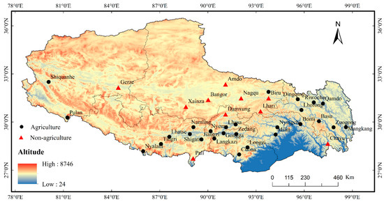
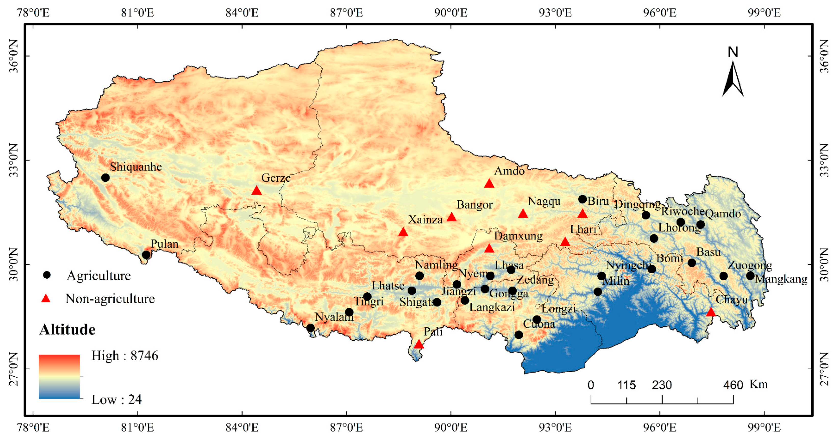
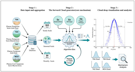
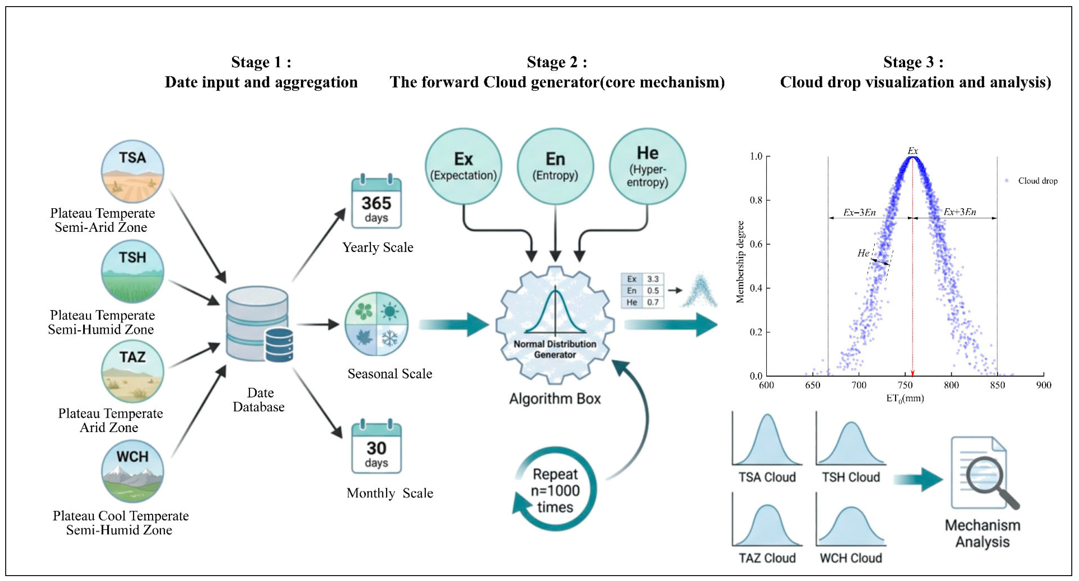
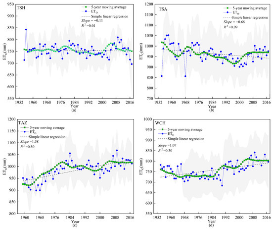
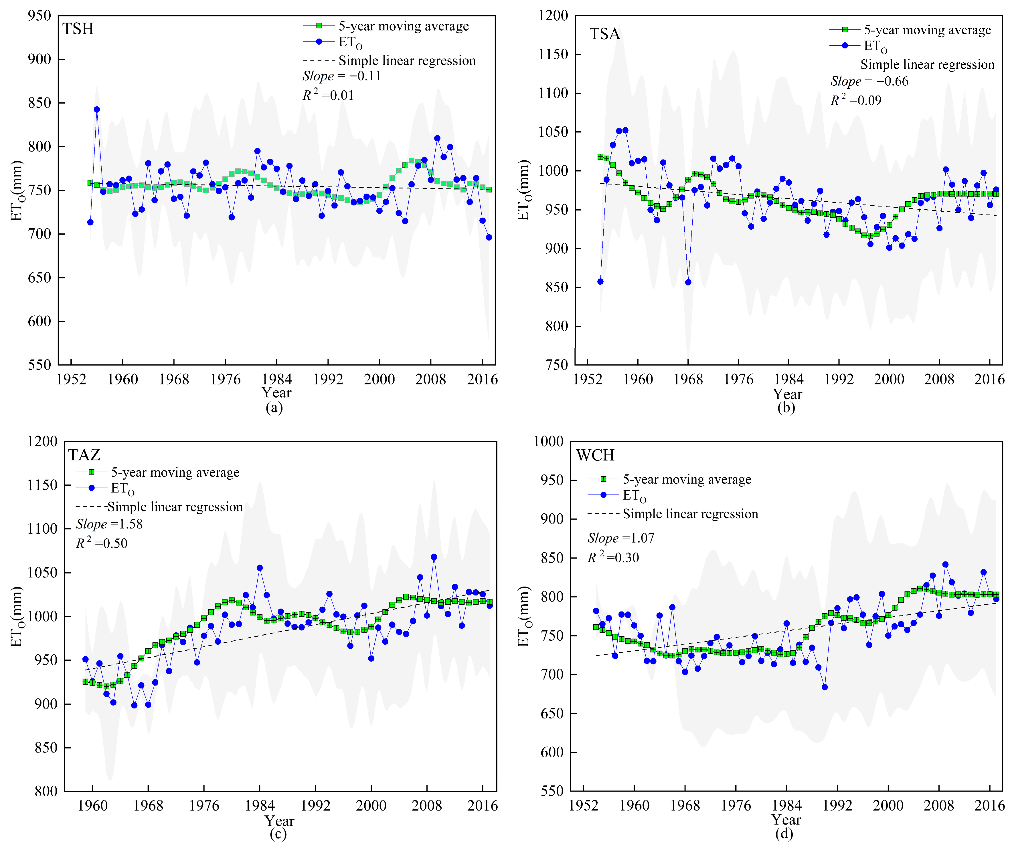
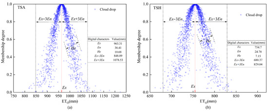
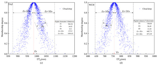
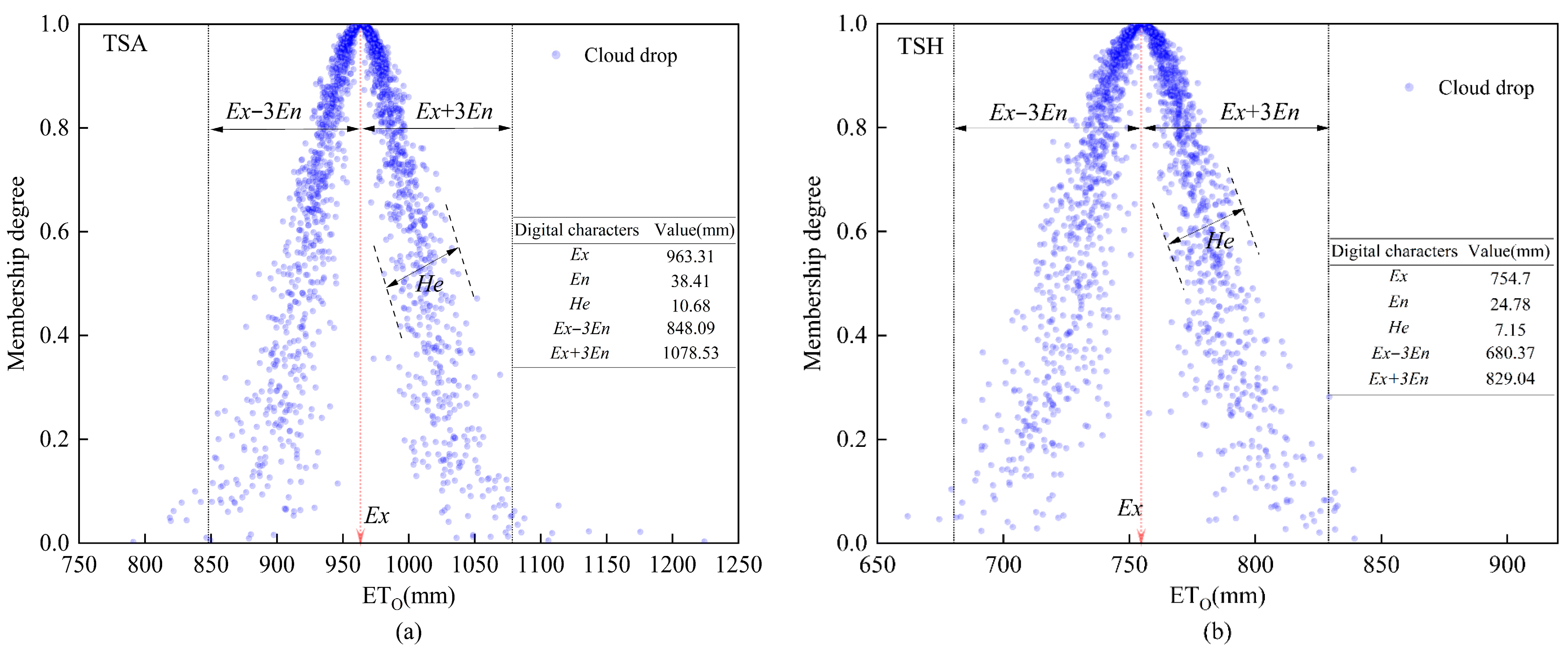
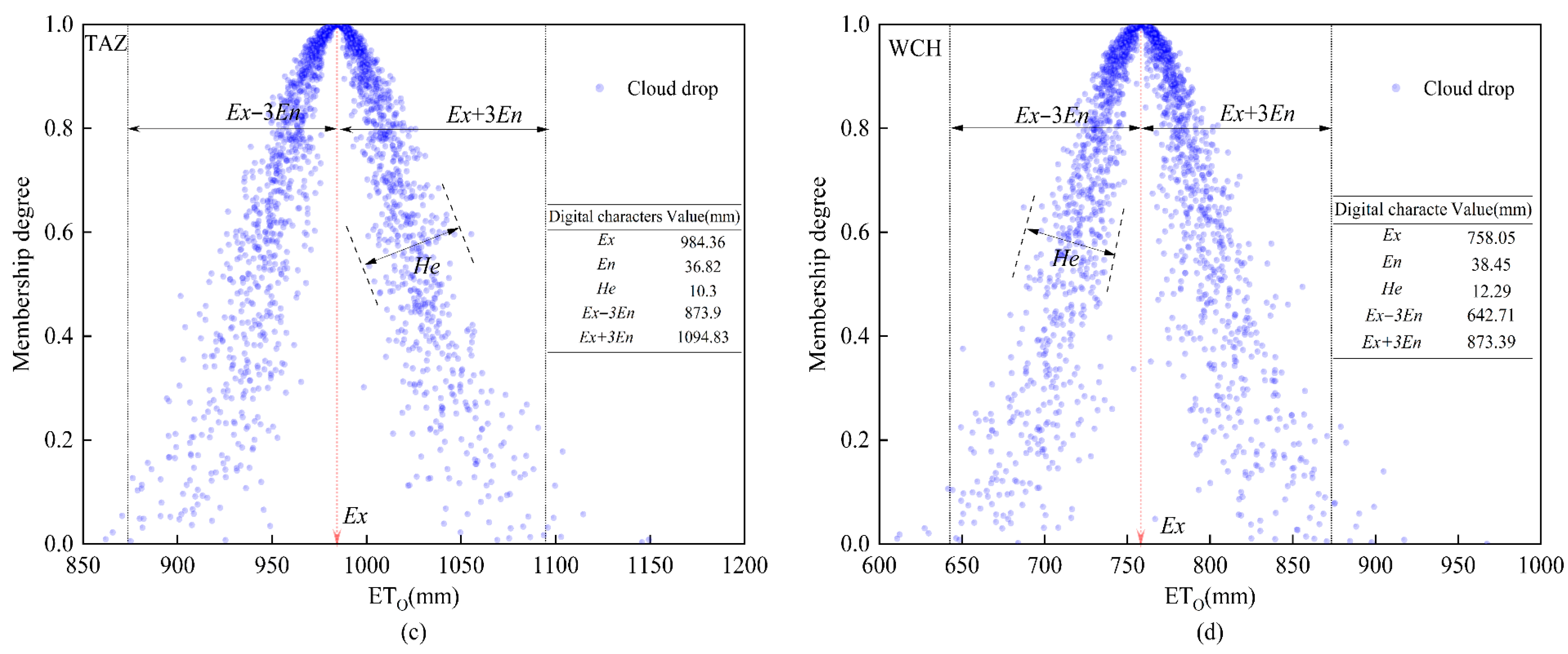
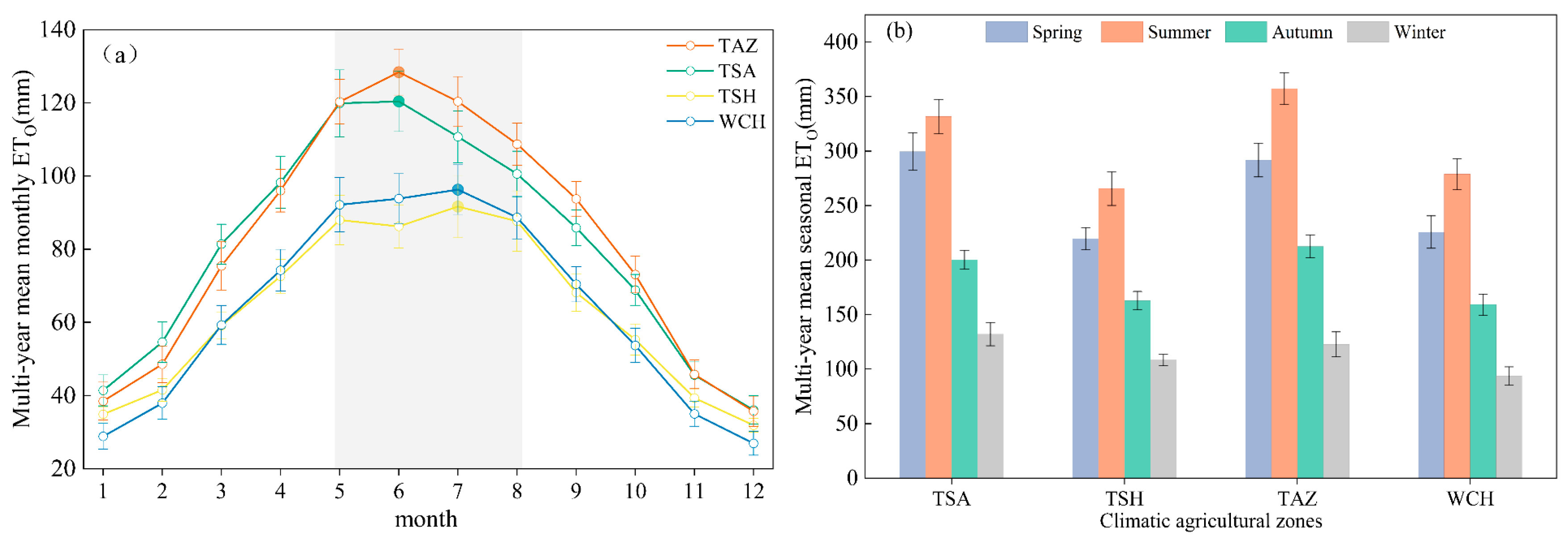
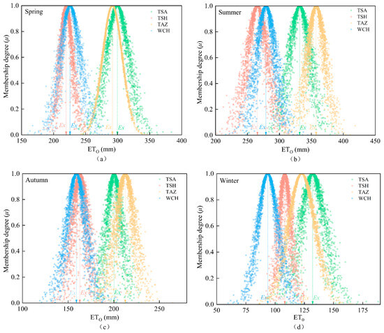
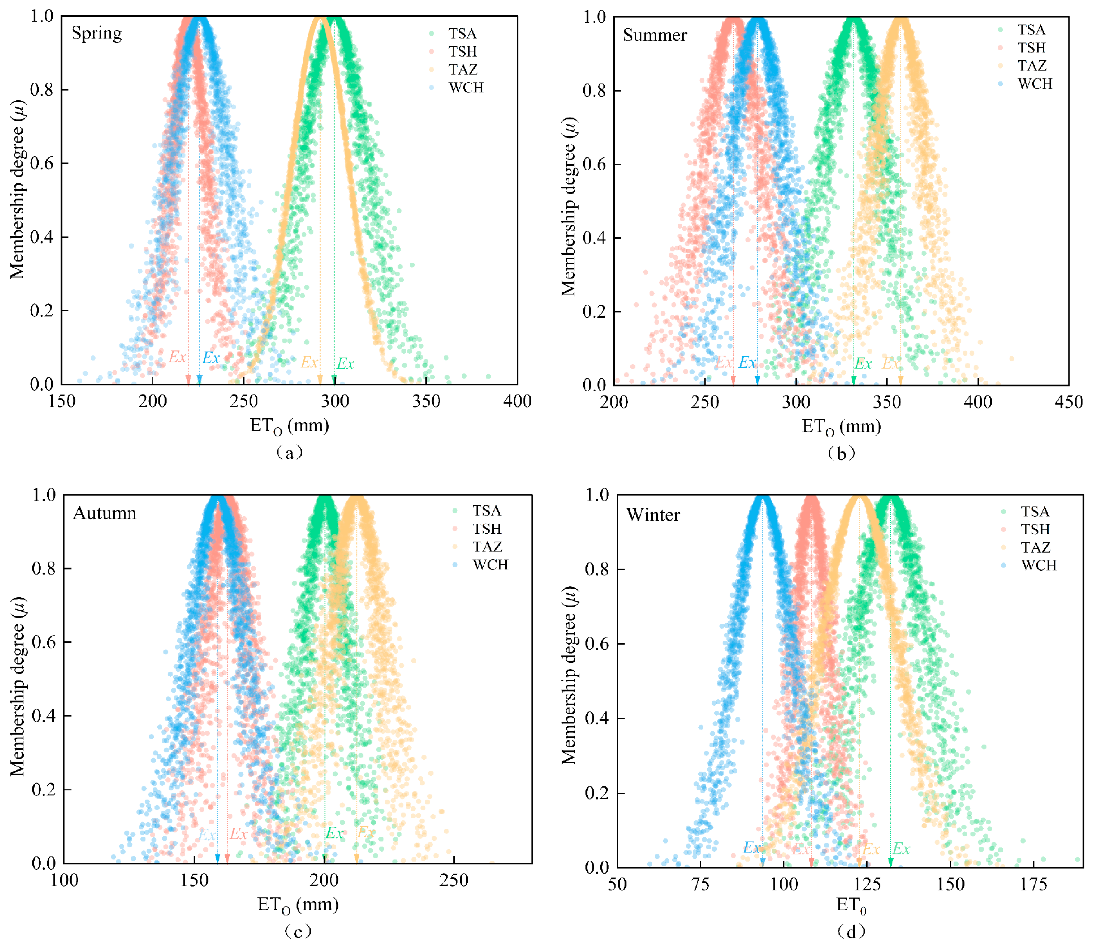
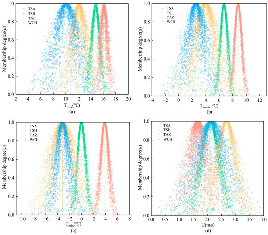
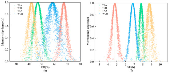
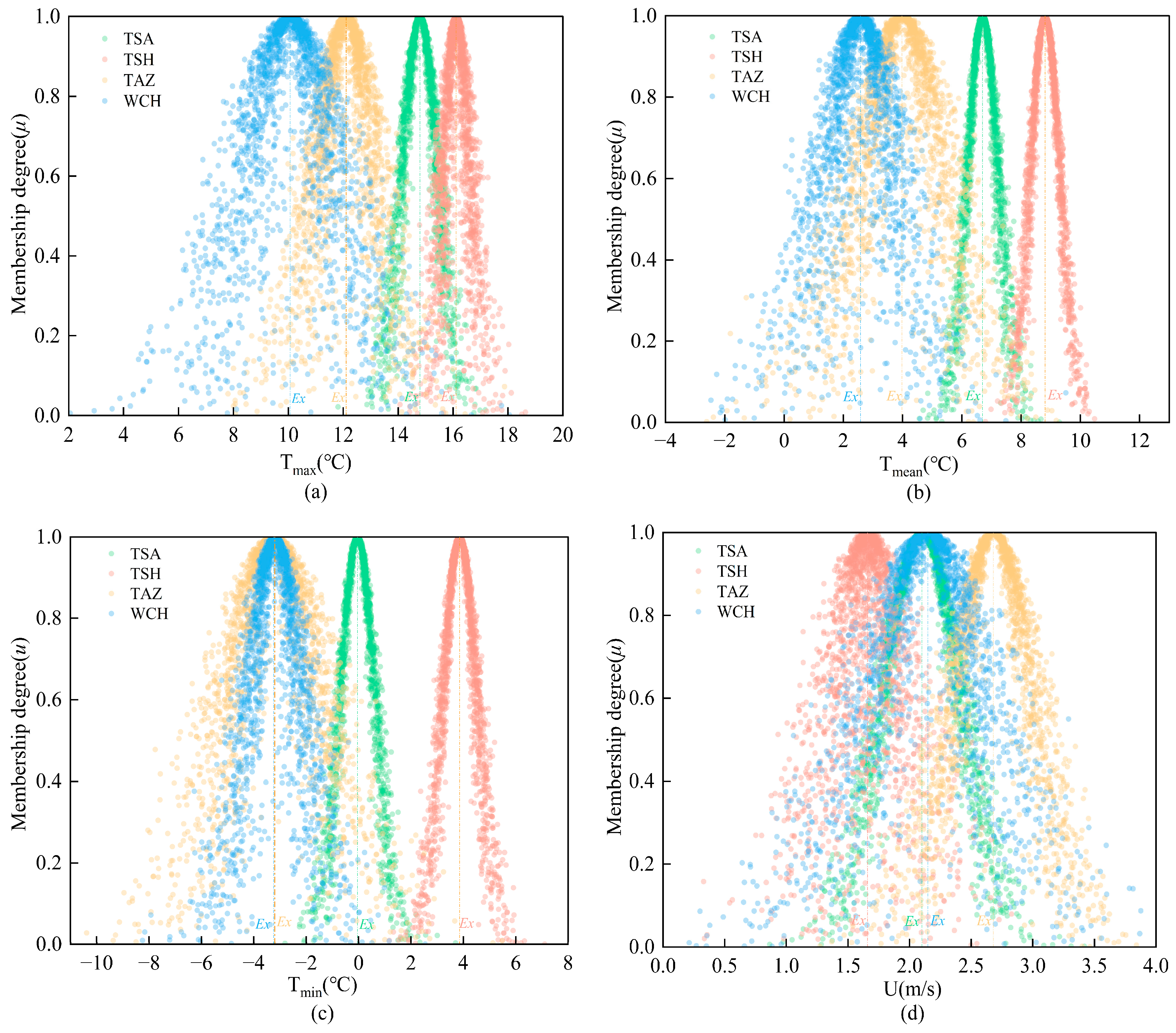
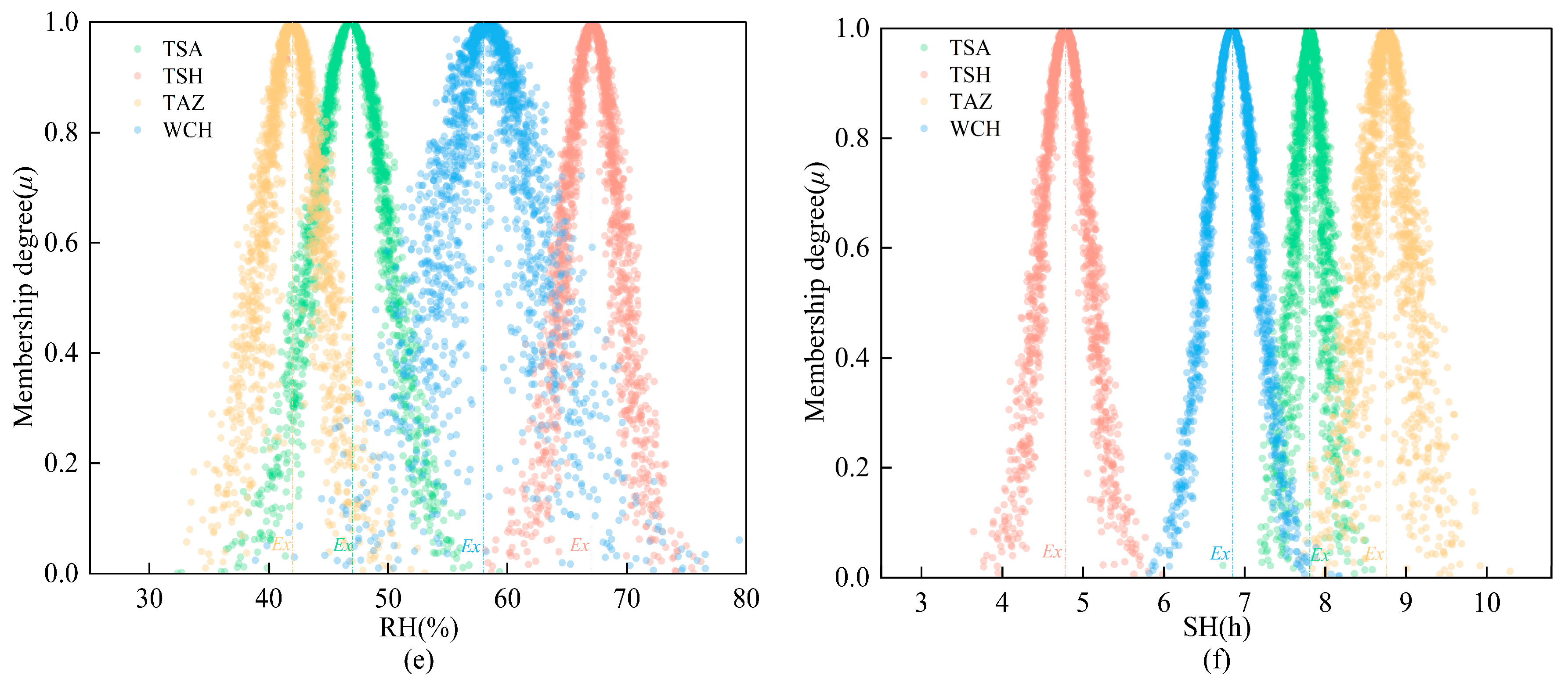
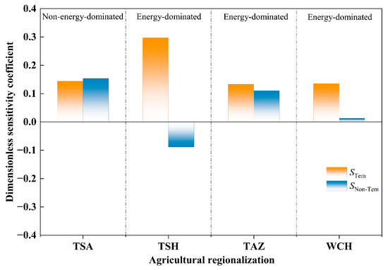
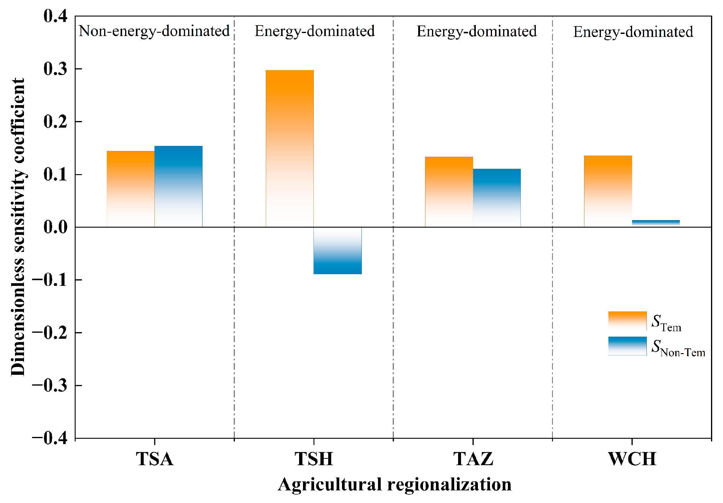
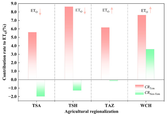
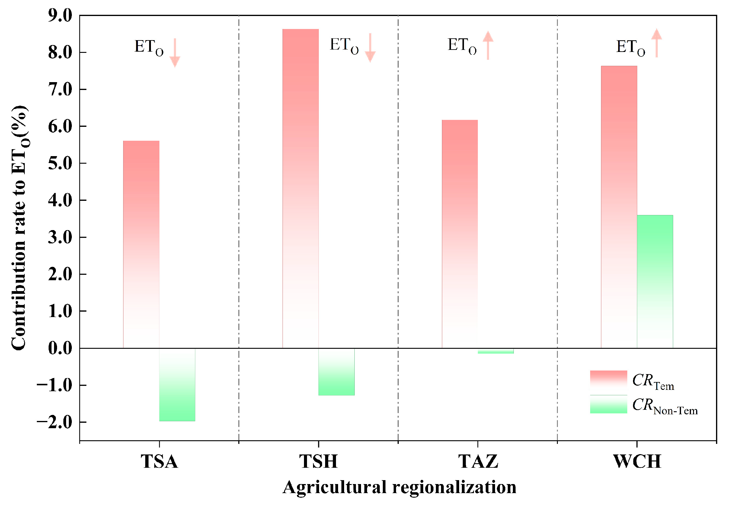
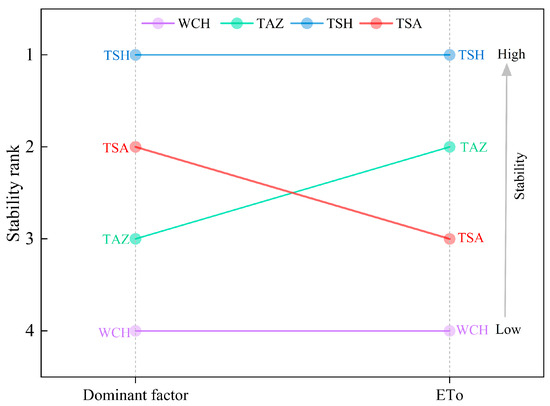
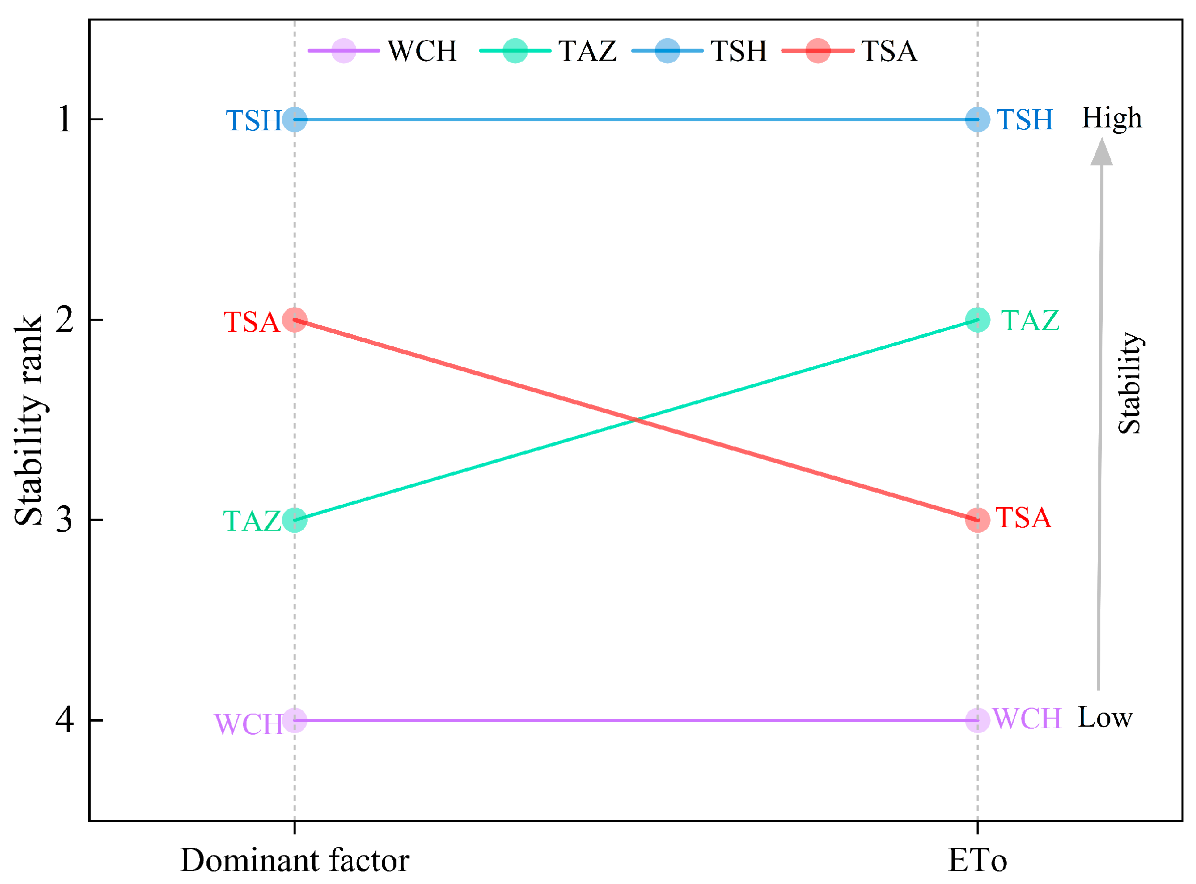
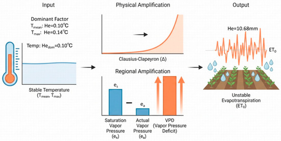
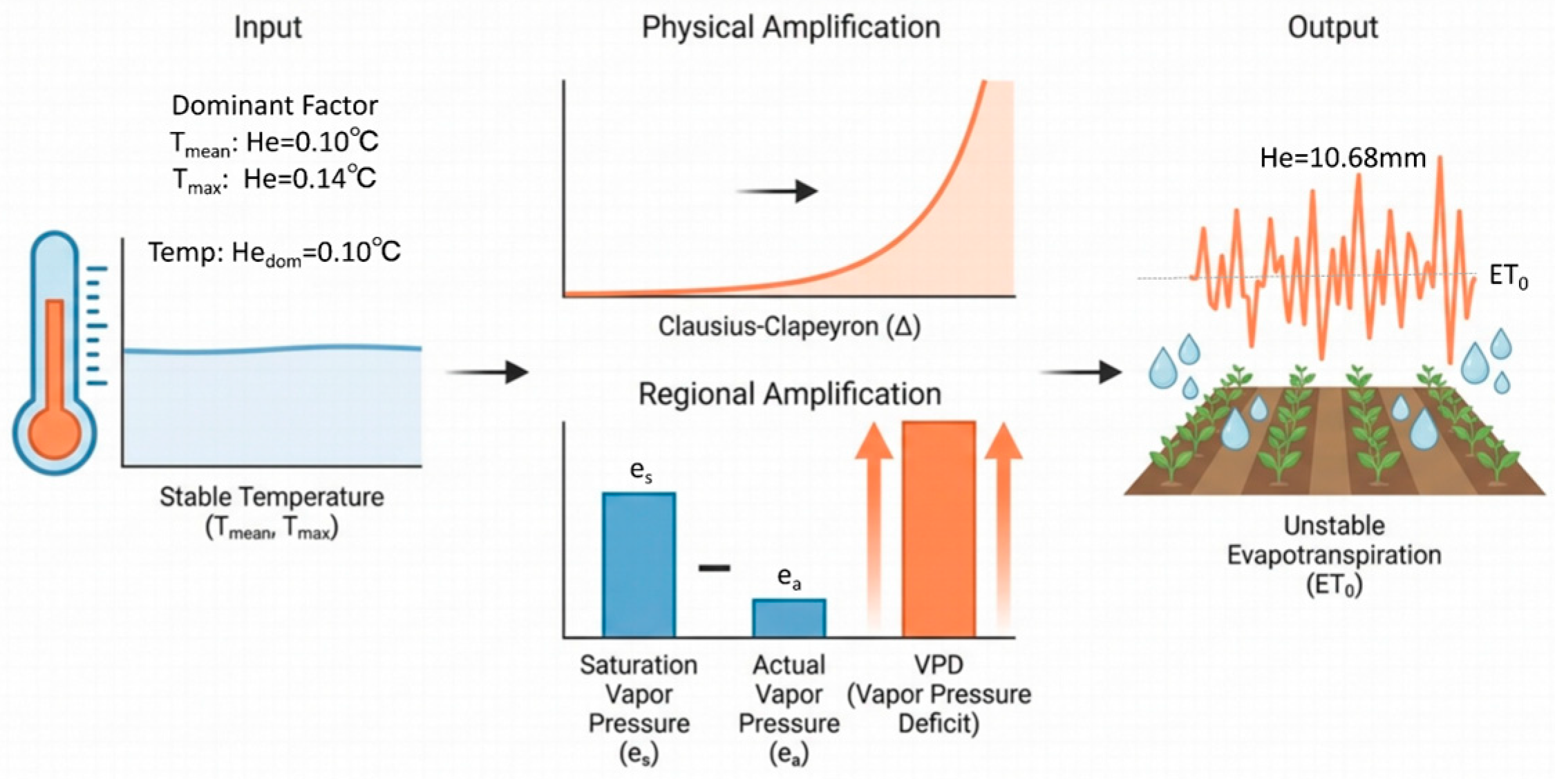
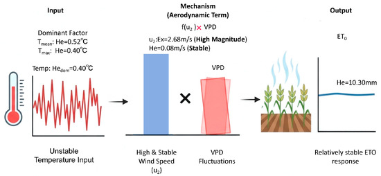
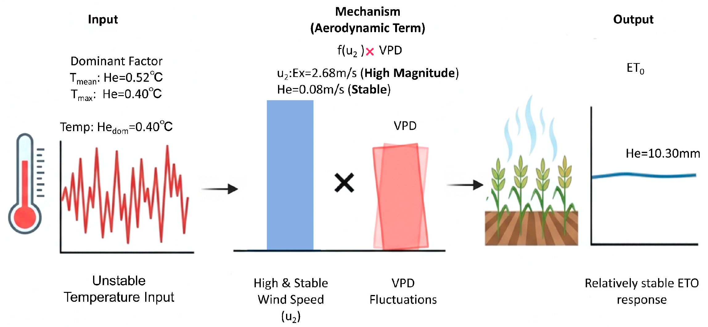

Disclaimer/Publisher’s Note: The statements, opinions and data contained in all publications are solely those of the individual author(s) and contributor(s) and not of MDPI and/or the editor(s). MDPI and/or the editor(s) disclaim responsibility for any injury to people or property resulting from any ideas, methods, instructions or products referred to in the content. |
© 2026 by the authors. Licensee MDPI, Basel, Switzerland. This article is an open access article distributed under the terms and conditions of the Creative Commons Attribution (CC BY) license.