


Highlights
- We show cases where tracking inundation with remote sensors is limited, particularly for medium-sized basins.
- We demonstrate that flood modeling is not merely complementary to remote sensing estimation, but essential for adequate flood risk assessment.
Abstract
This paper presents a comprehensive real-time forecasting and mapping cycle of a regional flood event, encompassing quantitative precipitation forecasting, runoff production and routing, and inundation mapping. The objective of this study is to highlight the significant uncertainties inherent in each step of the fully automated cycle, despite the utilization of state-of-the-art models and remote sensing technologies. The case study focuses on a significant flood event that occurred in the Turkey River and Upper Iowa River, in rural Iowa, United States, resulting in localized damage and disruption to several small communities. The novelty of this study is that it demonstrates the limited utility of satellite-based remote sensing in the absence of other forecasting and mapping system elements, emphasizing the need for the timely integration of information from diverse sources to accurately forecast and map floods. To achieve this, we assembled and analyzed precipitation data from weather radars, streamflow estimates derived from river stages and rating curves, and cross-sectional data from river channels to characterize the movement of the flood wave. These data were integrated into hydrologic and hydraulic models to generate flood inundation estimates for the more severely affected areas. Remote sensing imagery was obtained and used as reference to assess the accuracy of the modeled inundated areas. Our findings illustrate that, despite the increasing availability of satellite data sources, there are still significant limitations to tracking inundation using satellite remote sensing, particularly for medium-sized basins. Flood modeling processes are not merely complementary to satellite-based flood estimation, but essential for comprehensive flood risk assessment.
1. Introduction
Recent years have witnessed a surge of enthusiasm within the hydrologic research community regarding the potential of satellite remote sensing for flood mapping (e.g., ref. [1]). Similarly, flood prediction in the form of inundation mapping seems to be a new holy grail (e.g., ref. [2]) of the operational community. Real-time forecasting and mapping refers to the process of utilizing recent information to generate predictions and mapping of a system’s state over short-term horizons (ranging from hours to days). The key variable of interest in our study is streamflow, which, when exceeding the river channel’s conveyance capacity, results in flooding. Specifically, our investigation centers on riverine (fluvial) flooding, a critical aspect of flood risk assessment and management.
Our goal is to demonstrate that for satellite remote sensing of riverine systems to be useful in real-time monitoring, it must be complemented by an extensive system of models and data. We think this goal is important and novel, with little scientific literature on the topic as presented in our literature review later. The study also offers novel insights into the complexities of an effective flood forecasting system. To illustrate this argument, we selected a recent flooding event that occurred over a small region with medium-sized watersheds, representative of the majority of floods worldwide that impact local communities yet often remain “under the radar” of national media attention. Specifically, we selected an event that typifies the characteristics of most floods, which, while not catastrophic, still pose significant risks to local populations. We deliberately avoided flash-flood events, which are inherently unpredictable, ephemeral, and often lack sufficient observational data, thereby rendering them less suitable for illustrating the complexities of flood forecasting and mapping.
Our paper is organized chronologically along the timeline of a flood event, comparing precipitation/flood observations collected on the ground with the information provided by satellite observations that monitor these events and models that forecast their evolution. Through this framework, we show the limitations of the observational systems, both ground- and space-based; the interdependence of data and models; and most critically, the significant uncertainty that propagates through the entire forecasting system. Furthermore, the paper illustrates the complexity of the forecasting system, which in our paradigm is fully automated, thus there is no human expert intervention involved in the forecast-making process. While acknowledging that our study is a partial reconstruction based on real-time procedures, we aim to provide a nuanced understanding of the forecasting and mapping systems’ intricacies and challenges.
Most of the forecasting tools and data resources used in this study are identical to those used operationally at the Iowa Flood Center [3]. Specifically, these include the Hillslope–Link Model [4] that converts rainfall into runoff and route water through the river network, as well as flood inundation maps [5]. We also leveraged radar rainfall products derived from NEXRAD system data (e.g., ref. [6]) and quantitative precipitation forecasts issued by the National Oceanic and Atmospheric Administration [7,8]. Additionally, we reviewed forecasts from the National Water Model (e.g., ref. [9]) although, for the sake of brevity, these results are not presented here. In this study, we focus on the rainfall–runoff model as a generic element of streamflow forecasting systems.
At this point we note that forecasting a dynamic system with external forcings requires the forecasting of the forcings themselves. If this condition is not met, we have a case of simulating the system’s response to an observed forcing. While the response may extend into the future, simulating it is not forecasting. We stay consistent with this definition of forecasting, which eliminates a large body of the literature from our scope as many studies use the term “forecasting” but, in fact, describe simulation.
We analyzed the most recent scientific literature that conducted real-time hydrologic forecasting of flood events. These studies encompass a wide range of basin sizes, from storms in small basins [10,11] to large basins affected by hurricanes or typhoon events [12,13,14]. In general, studies suggest that the main challenges in real-time streamflow forecasting arise from operational systems that rely on a small number of numerical weather prediction inputs [11], the added complexity of simulating streamflow in mountainous terrain [10,15,16,17], the short response times of small and urban basins and the high computational demand to model these [18,19]. Challenges also arise from the high variability of precipitation forecasts between cycles, and the uncertainty of the rainfall inputs [13,14,17,20,21,22,23,24,25,26,27]. The rainfall forecast uncertainty is related to multiple sources of error including the overestimation at short lead times [25]; errors in the location of predicted storms [14,21,26]; over- and underestimation of storm events [10,12,21,23]; overestimation of larger-scale events like typhoons and hurricanes [13,14]; the large spread of rainfall ensembles [14]; and errors in predicting the timing and spatial distribution of convective storms [19,20].
Real-time flood monitoring systems use information from flood forecasts from hydrologic models, combined with the monitoring of flood extents using optical imagery [28,29,30,31] or synthetic aperture radar measurements [32]. The main challenges from flood monitoring emerge from the cloudy conditions common during floods, coarse spatial resolution from satellite imagery, temporal gaps due to long revisit times, misclassification of flooded areas, and detection of flooded areas under dense vegetation or urban structures [28,29,30,31].
Flood Event and Area of Study
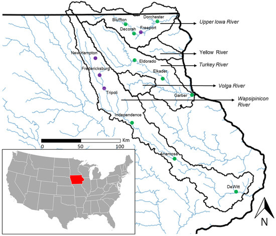
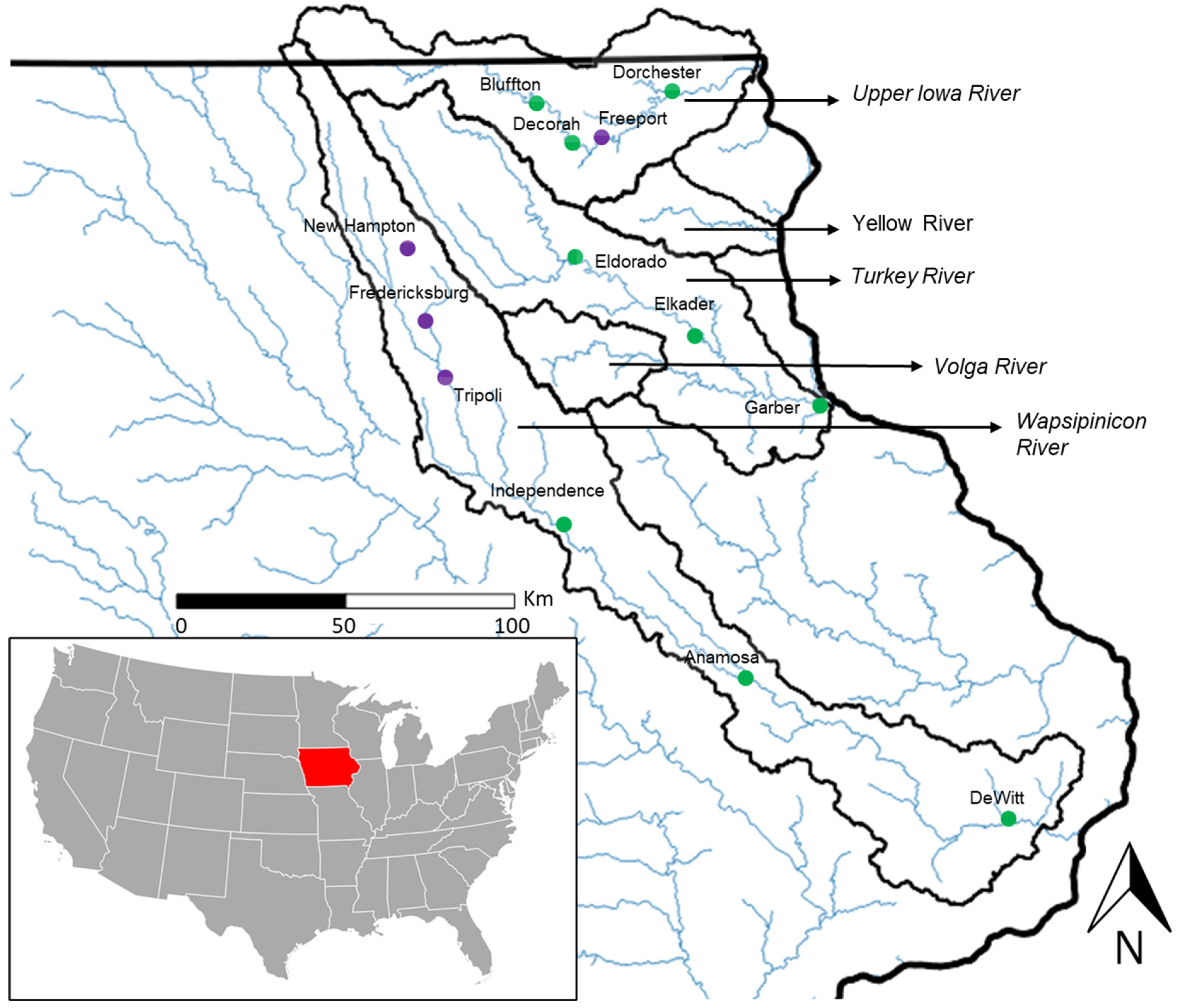
A severe storm swept through northeastern Iowa during the night of 27 August and morning of 28 August 2021, bringing heavy rainfall that caused significant flooding in five watersheds: the Upper Iowa River, Volga River, Yellow River, Wapsipinicon River, and Turkey River (Figure 1). The basin’s physiography is characteristic of the Paleozoic Plateau landform, with steep hills, deep valleys, and streams with steep gradients resulting in fast-moving waters.
Figure 1.
Area of study and locations of the selected sites and basins. The purple dots show the affected communities and green dots show USGS sensors.
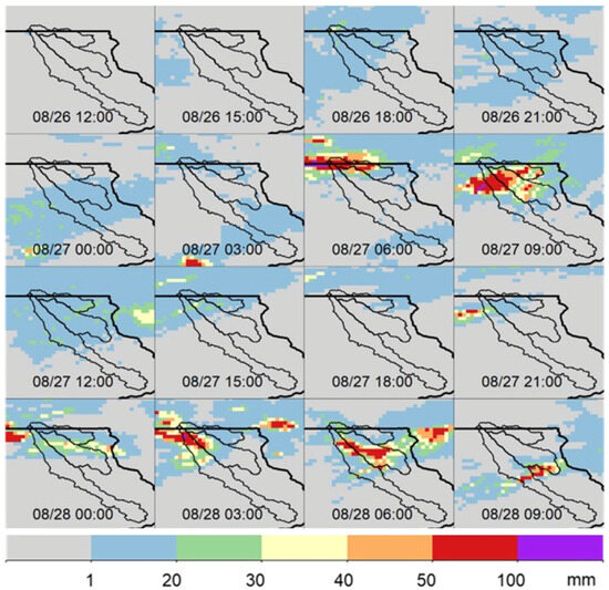
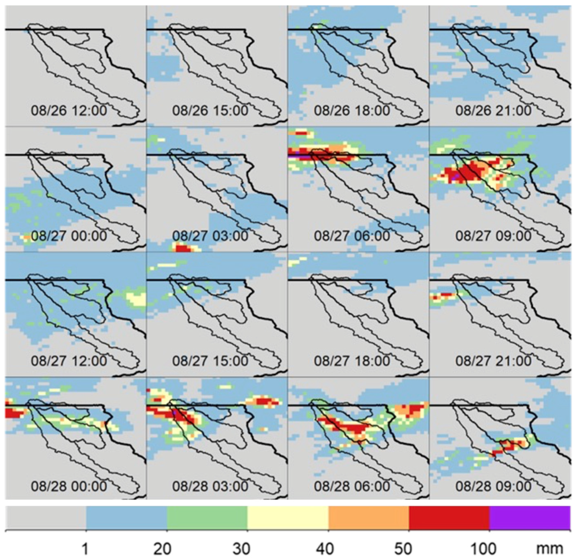
Based on weather radar observations, the National Weather Service (NWS) reported accumulated rainfall totals ranging from 75 to 200 mm across north-central Iowa, with peak intensities reaching over 50 mm/h during a three-hour period on the morning of 28 August (Figure 2).
Figure 2.
Three-hour accumulations of observed MRMS radar rainfall product from August 26 to 29 in northeastern Iowa.
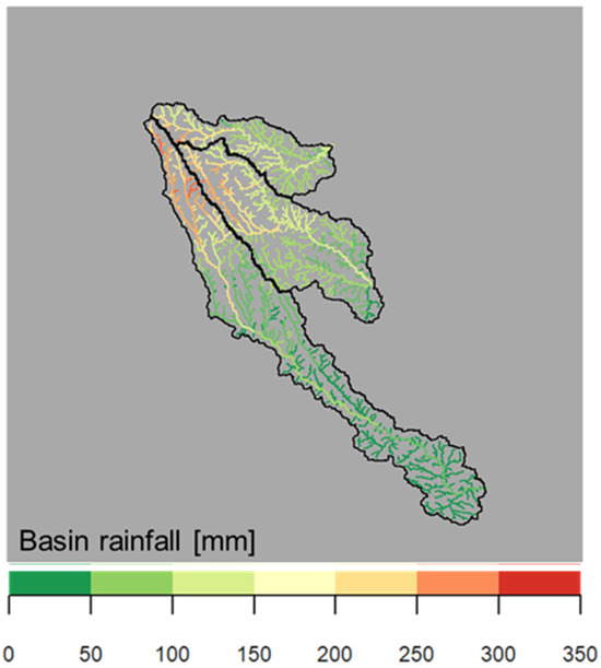
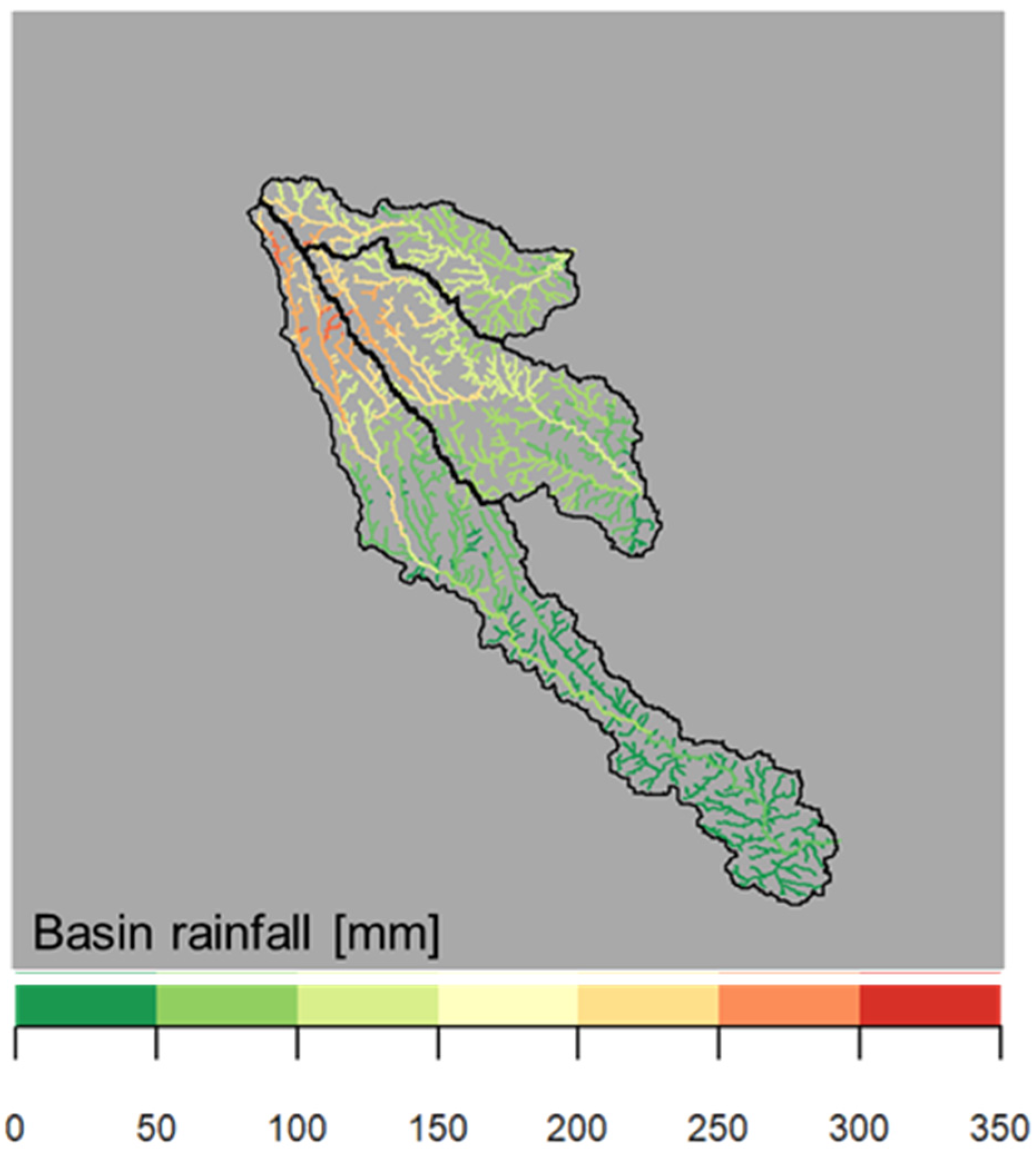
Local rain gages recorded even higher totals, exceeding 250 mm in some areas. Figure 3 presents a three-day cumulative radar rainfall total for 26–29 August, visualized as a color-coded river network that illustrates the mean areal rainfall upstream from each segment.
Figure 3.
Three-day radar rainfall accumulation shown as mean areal precipitation for every subbasin in the domain of interest for (from top: Upper Iowa River, Turkey River, and Wapsipinicon River. The rainfall amount over each subbasin is represented as a color-coded river network link draining that subbasin.
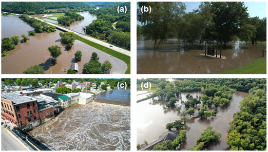
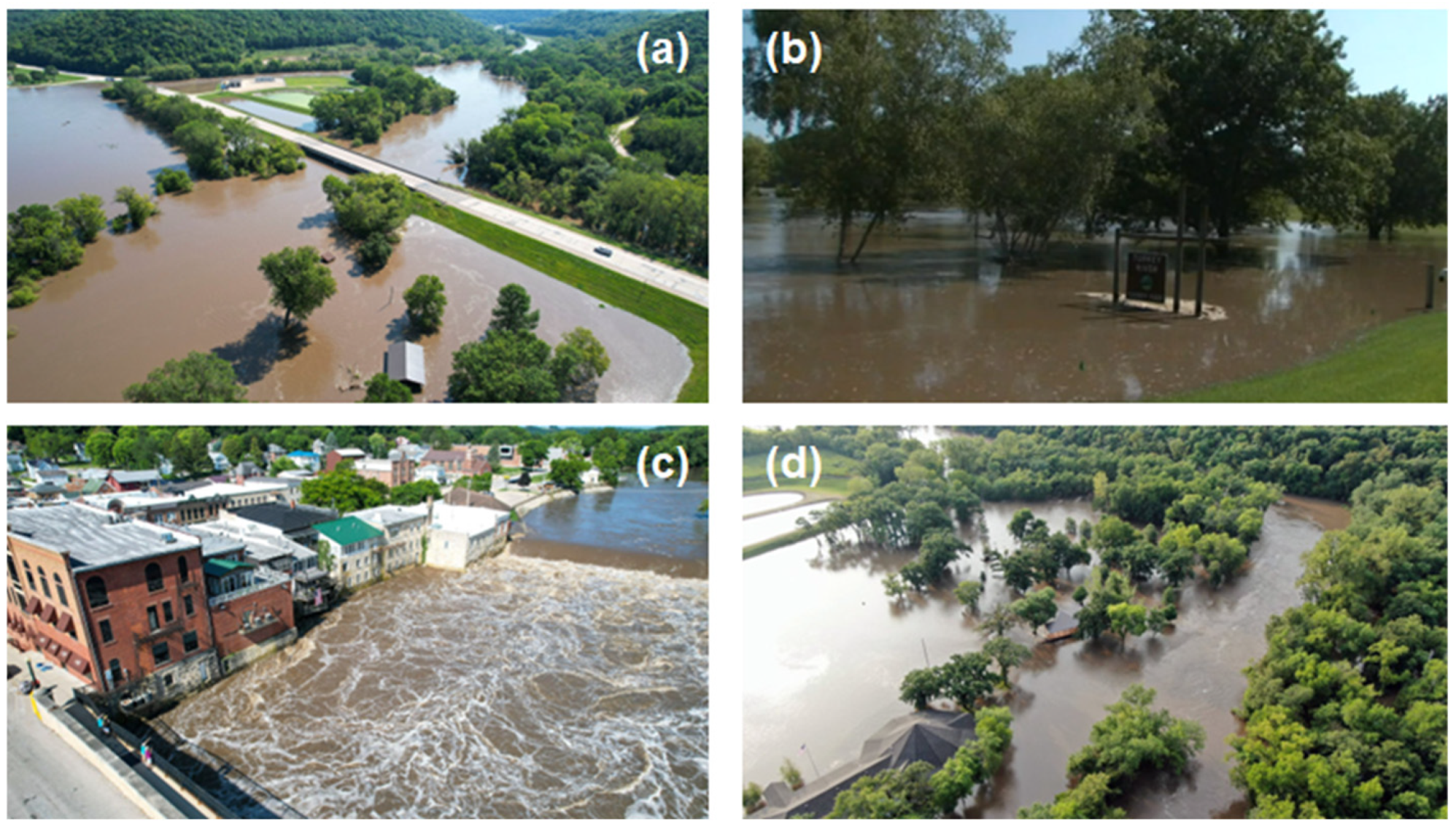
Intense rainfall triggered a rapid rise in river levels, with many stream gages reaching alarmingly high levels. In the Wapsipinicon River, water levels at Independence surpassed the moderate flood stage by 0.5 m, while at Tripoli, river stages approached near-record levels less than 48 h from the start of the storm. Peak flows reached their maximum values on 28 August in most of the upstream basins and on 30 August in most of the downstream basins. Roads and major highways in northeastern Iowa, including Iowa Highway 9 west of Decorah and U.S. Highway 18 west of Fredericksburg and New Hampton, had to be closed due to flooding. The crest in the Turkey River at Elkader was the fourth highest on record at nearly 7 m. The community of Elkader had been affected many times in the past, with floods in 2008, 2010, 2011, 2014 and 2016. The 2021 event proved just as destructive, causing damage to public property, recreational trails, and areas along the riverbanks as illustrated in Figure 4.
Figure 4.
(a) River crest at Elkader (photo: Telegraph Herald), (b) Turkey River County Park (photo: KCRG-TV9), (c) Turkey River at Elkader, Iowa, on 30 August 2021 (photo: Telegraph Herald), (d) Flooding in Winneshiek County (Upper Iowa River) on 28 August 2021 (photo: Winneshiek County Emergency Management).
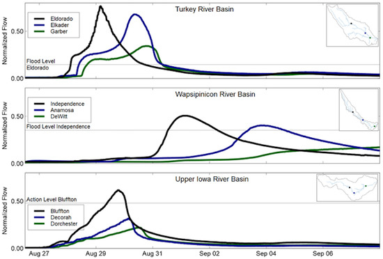
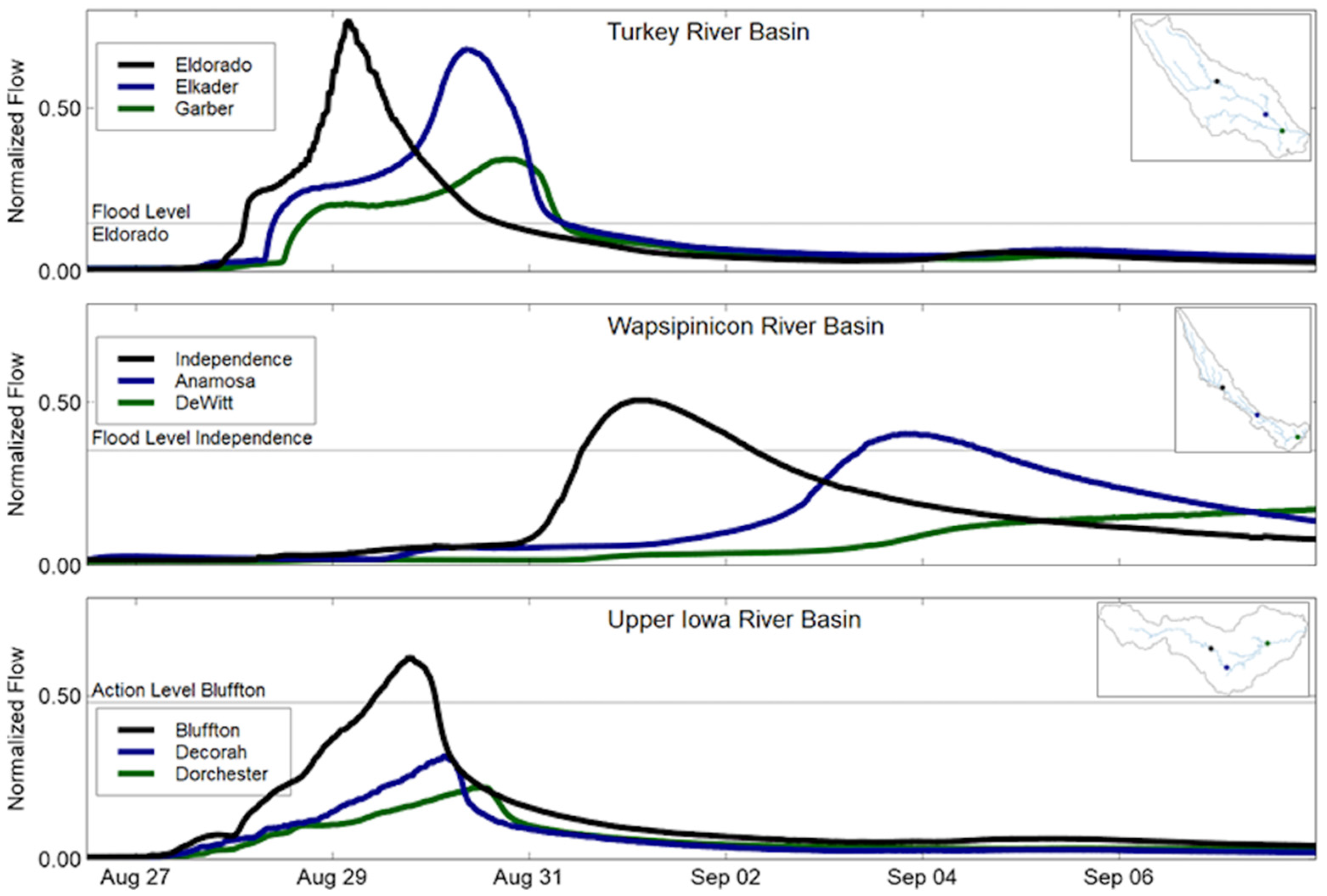
For this study, we selected a ten-day period from 25 August to 3 September to examine the event in detail. This timeframe enabled us to consider the pre-event streamflow and soil moisture conditions, providing a comprehensive understanding of the event’s context. We selected two severely affected locations, the Upper Iowa River at Decorah (1320 km2) and Turkey River at Elkader (2330 km2), based on the availability of observed data and inundation maps derived from streamflow observations from the United States Geological Survey (USGS), which served as the basis for our analysis. Figure 5 presents a time series of streamflow at locations where there is information available, illustrating the evolution of the event over time.
Figure 5.
Hydrograph-observed streamflow from 25 August to 3 September 2021, at the USGS stream gages in the respective basins. The flow is normalized by the mean annual maximum flow.
2. Materials and Methods
2.1. Precipitation Estimates and Forecasts
Quantitative precipitation estimates (QPE) are radar-based from the Multi-Radar Multi-Sensor (MRMS) precipitation product [6] that quantifies the intensity and location of storm events. The operational MRMS system is a state-of-the-science hydrometeorological data analysis and nowcasting framework that combines data from multiple radar networks, satellites, surface observational systems, and numerical weather prediction models, to produce a suite of real-time decision support products every two minutes over the contiguous United States and southern Canada [33]. In this study we used the 1 km spatial resolution, hourly rainfall maps with rain gage correction applied.
Quantitative precipitation forecasts (QPF) were obtained from the High-Resolution Rapid Refresh (HRRR) numerical model [7]. HRRR is a convection-allowing atmospheric model developed by the National Oceanic and Atmospheric Administration (NOAA). It has a horizontal grid spacing of about three kilometers and is updated hourly, providing detailed forecasts of weather conditions over the United States and Alaska for the forecast lead time of up to 18 h.
2.2. Satellite Images
We explored satellite imagery availability for the locations and the time period of this study. We used PlanetScope images that were available for the selected sites, which were captured on the same day that the rivers reached their peak flow, although not at the exact time. Specifically, the images for the Turkey River site were taken two hours after peak flow, while those for the Upper Iowa River sites were taken between 4 and 8 h after peak flow. We used these images for the study since they provide the best resolution at the selected sites and dates. We also explored Sentinel 2, Landsat 8 and SkySat products but there were many limitations due to cloud cover and satellite revisit time. We provide more details of the satellite products in Appendix A.
2.3. Rainfall–Runoff Models
We used the Hillslope–Link Model (HLM) developed by the Iowa Flood Center to generate streamflow forecasts. The HLM is a continuous rainfall–runoff model that simulates hydrologic processes by decomposing the landscape into hillslopes and channel links. The model is formulated as a system of ordinary differential equations (ODEs) that describe the changes in water stored in soil and the river network. The HLM configuration in this study uses four storages: (1) water ponded in the soil surface of 2 cm depth; (2) soil moisture stored in the upper layer of soil of 50 cm depth; (3) soil moisture stored in the lower layer of soil; and (4) water stored in the channels. The infiltration process between soil layers is nonlinear, which makes the soil act as a memory element that controls the dynamics of runoff generation. The ODEs are solved using a parallel implementation of Runge–Kutta methods that allow for asynchronous integration. HLM simulations were conducted at every hillslope–link pair in the river network of the Turkey River and the Upper Iowa River basins. The model is calibration-free, meaning that its parameters are determined a priori, and not changed for specific basins or model forcings. The model is forced with observed rainfall from Multi-Radar Multi-Sensor (MRMS), and evapotranspiration estimates from Moderate Resolution Imaging Spectroradiometer MODIS [34]. The HLM estimates hourly soil moisture states. For streamflow forecasting, the model was forced every hour with precipitation forecasts from the High-Resolution Rapid Refresh (HRRR) of 18 h duration. The model integrates the precipitation forecast and projects the streamflow response for the next five days.
2.4. Open Channel Flow Models
We developed one-dimensional numerical open channel models for the Turkey and Upper Iowa rivers using HEC-RAS Version 6.3.1. The software is capable of simulating unsteady flow based on the section-averaged Saint-Venant equations. One-dimensional solutions of the Saint-Venant equations rely on geometric features defined by a series of carefully selected channel cross-sections [35]. We performed unsteady flow analysis to simulate the period between 25 August and 3 September using the computational interval of 15 s and the output interval for hydrograph plotting and inundation mapping of 15 min. We used highly detailed and accurate geometry cross-sectional data and stream centerlines for the Upper Iowa and Turkey rivers using airborne LiDAR data. For the flood plain, Manning’s roughness values were selected based on typical values recommended by [36], while a value of 0.035 was selected for the entire channel based on experience at neighboring basins and field work [5]. The one-dimensional hydraulic model for the Turkey River simulates the reach between the USGS stream gage at Eldorado as the most upstream point, and the Garber USGS gage as the most downstream point, with a river length of approximately 330 km (Figure 1). We used the flow hydrograph observed during the time of the event at the USGS Turkey River station near Eldorado (USGS code 05411850) as the upstream boundary condition. The downstream boundary condition was established as the normal depth at the USGS Turkey River station at Garber (USGS code 05412500) using the channel slope as reference.
The configuration of the one-dimensional hydraulic model for the Upper Iowa River simulates the reach between the USGS gage at Bluffton as the most upstream point, and the Dorchester USGS gage as the most downstream point, with a length of approximately 89 km (Figure 1). Model results were obtained at the USGS gage at Decorah 28 km downstream from Bluffton. The upstream boundary condition was the flow observed at the USGS Upper Iowa River location at Bluffton (USGS code 05387440). The downstream boundary condition was the normal depth at the USGS Upper Iowa River near Dorchester (USGS code 05388250) using the channel slope as reference.
For comparison, we also developed two-dimensional numerical models for the Turkey and Upper Iowa rivers using HEC-RAS Version 6.3.1. HEC-RAS utilizes a high resolution subgrid model, allowing each computational cell and cell face to use details of the underlying high-resolution topography [37]. High-resolution DEMs contain all necessary geometry information to create computational meshes. As for the one-dimensional model we discussed above, we set the spatially varied Manning’s roughness values based on typical values recommended by [36] and parameterized by high-resolution land cover (HRLC) classifications. We used the default diffusive wave equations for the simulations due to subcritical flow conditions, relatively low velocities and gradual flow fluctuations present in the model domain. For the setup of the two-dimensional models of both basins, we used a one-meter-resolution DEM to create a 2D structured computational mesh of ten-meter resolution. For the Turkey River in particular, we set the mesh to three meters for the main channel section. We performed an unsteady flow analysis between 25 August and 3 September 2021, with the period between 17 August and 24 August used for model initialization and spinup. The computation interval was set to 15 s and the time intervals for hydrograph and mapping outputs were 30 min. For the Turkey River model, the upstream boundary condition is the observed flow at the Eldorado streamgage and the downstream boundary at the Garber streamgage is the normal depth. For the Upper Iowa River model, the upstream boundary condition is the observed flow at the Bluffton streamgage and the downstream boundary at the Dorchester streamgage is the normal depth.
3. Analysis
As the late-August 2021 event unfolded, initial radar observations revealed a severe storm progressing across the northeastern region of the state. This section analyzes the storm’s forecast accuracy in depth, leveraging observations—both ground- and space-based—models, and model-based data resources to reconstruct the event timeline. Our goal is to effectively contextualize the value of satellite remote sensing in a proper perspective for a flood forecasting problem.
3.1. Predicting the Response
We used the HLM to forecast landscape responses to heavy rainfall. Initially, we demonstrate the HLM’s ability to integrate responses when past (up to the point of issuing a forecast) rainfall is available. This integration is facilitated by the model’s set of differential equations, which need to be solved given the initial conditions and account for the hydrologic system’s delayed response. Notably, this process is technically not forecasting unless it is assumed that no future rainfall will occur, which is not the case here.
To extend the streamflow projection, the hydrologic model must use a rainfall forecast, or Quantitative Precipitation Forecasting (QPF). However, rainfall forecasts are subject to considerable uncertainty, especially as rainfall–runoff models require accurate quantification of “when”, “where”, and “how much”. Note that the QPF skill is spatial scale-dependent (e.g., ref. [25,38,39]). It is “easier” for large basins to “tolerate” forecast errors, especially those in spatial storm placement. The skill is also strongly lead time-dependent. It is easier to forecast for the next hour than for the next day.
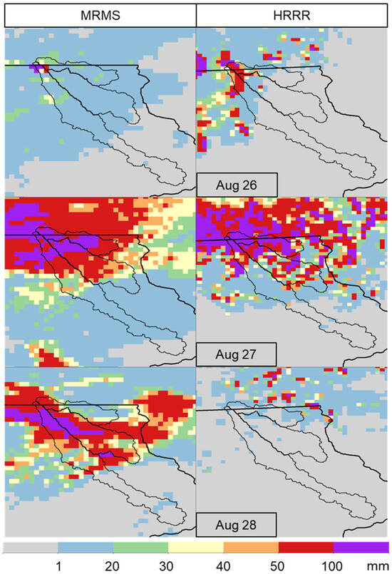
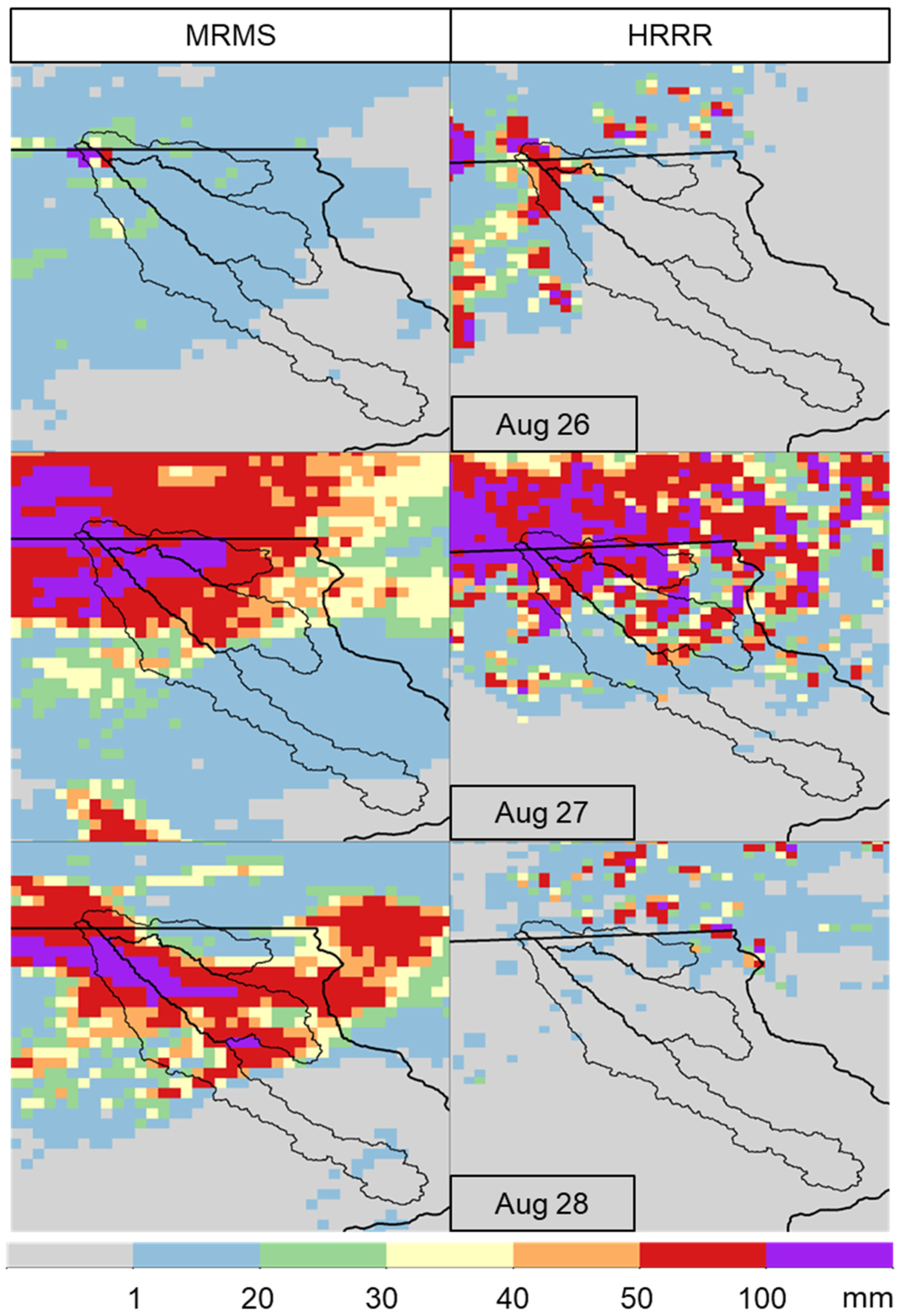
We present a case of streamflow forecasting to illustrate the potential utility of good QPF and the pitfalls of poor forecasts. First, let us look in Figure 6 at the comparison of observed radar rainfall of the MRMS and a high-resolution QPF product known as HRRR. The HRRR QPF is issued every hour up to 18 h ahead with an hourly resolution. Therefore, there are 18 values of rainfall forecasted for each location (pixel). Each time a new QPF is issued, it is used to force the hydrologic model and a new streamflow hydrograph is produced. Because of this multiplicity of the space–time arrangements of the QPF vs. QPE, it is difficult to graphically illustrate the skill of the QPF. For a comprehensive discussion, readers are referred to ref. [38]. Here, in Figure 6, we show a simple illustration of the issue selecting just one of the forecasts and comparing it to the radar-estimated rainfall. As the basin’s total rainfall volume is the most important variable that determines basin response, we compare 18 h of accumulation of rainfall over the region.
Figure 6.
Side-by-side comparison of the MRMS and HRRR. The MRMS data were upscaled to match the HRRR grid spacing. Shown are the first 18 h accumulations for each day.
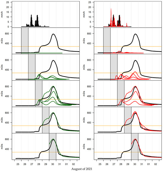
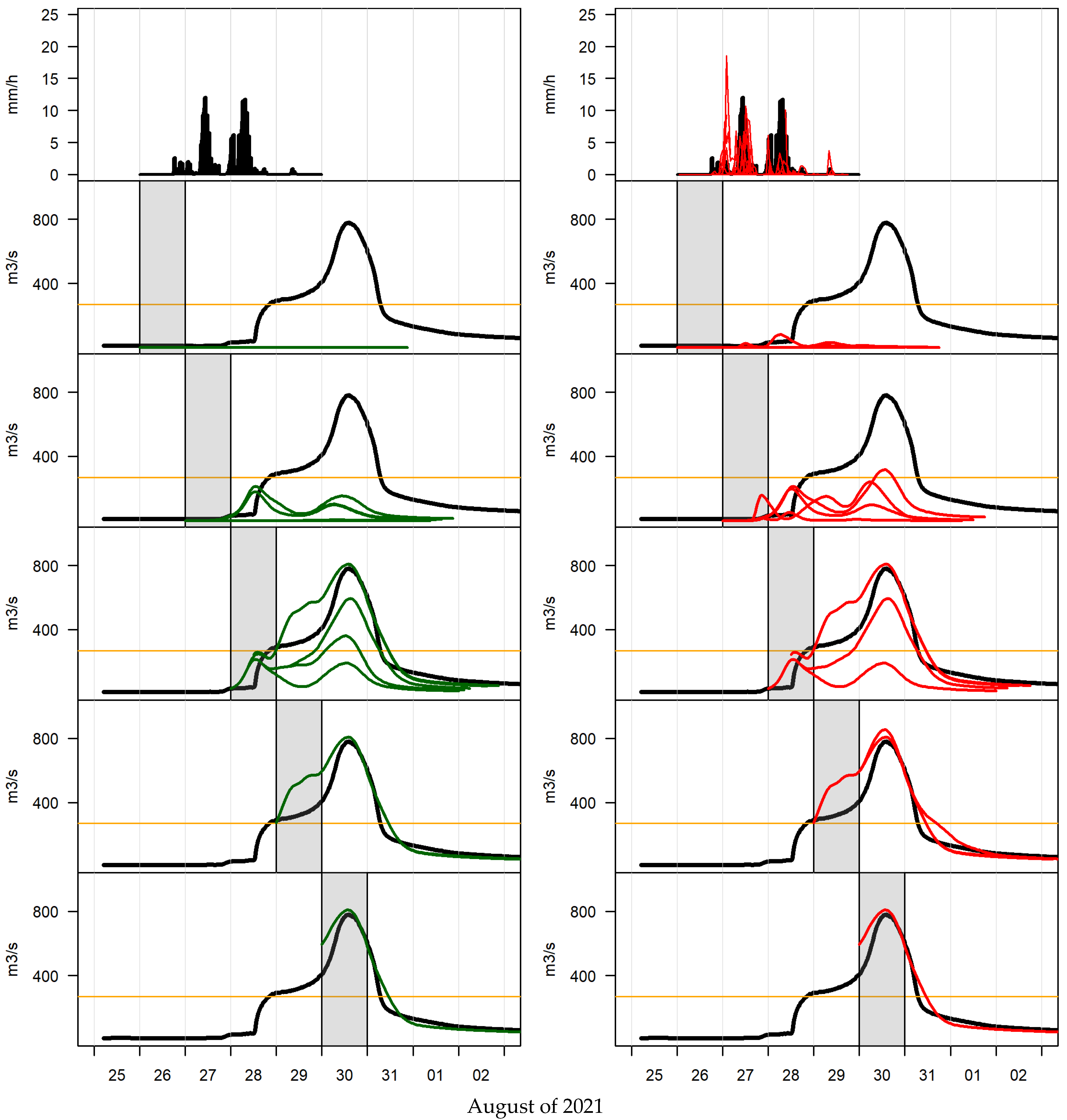
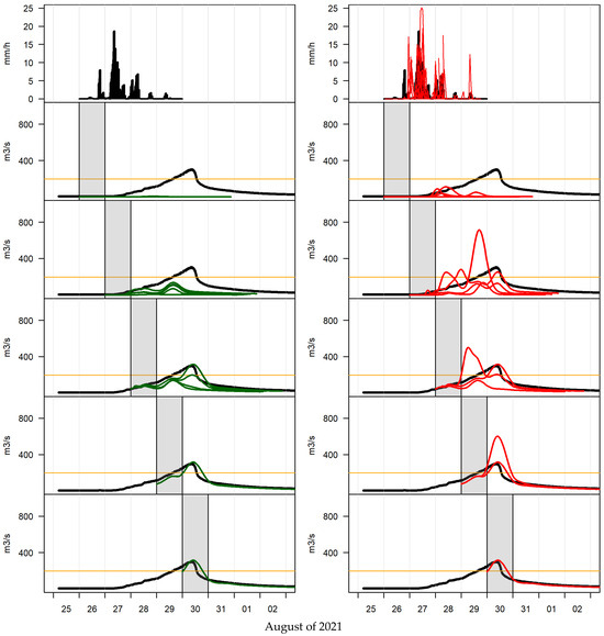
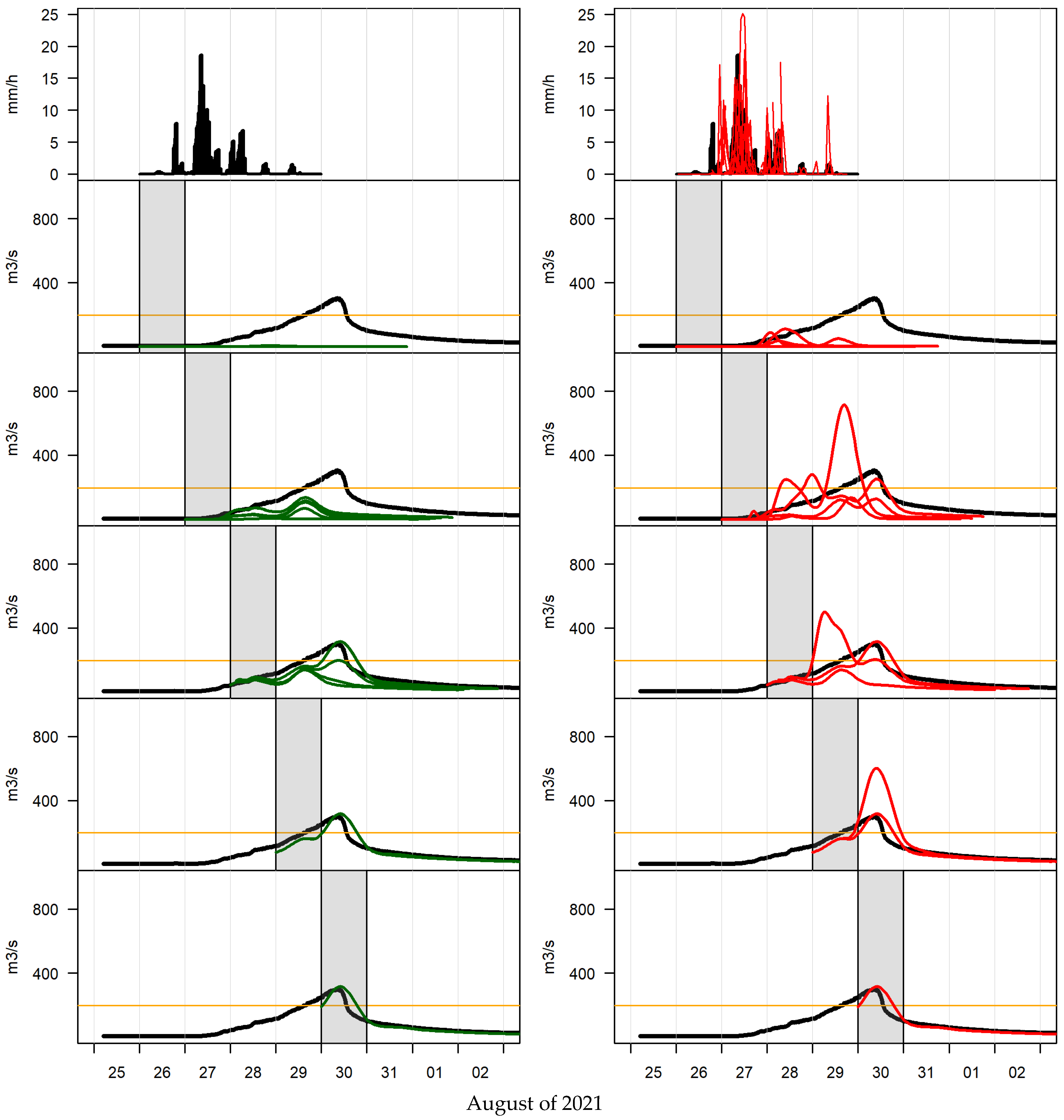
What are the consequences of such rainfall forecasts for streamflow forecasts? Consider the problem in the time domain at two locations: outlet gage sites for Elkader on the Turkey River and Decorah on the Upper Iowa River. We present the results in Figure 7 and Figure 8, respectively. The top panels show a time series of the basin’s mean hourly rainfall, as estimated from radar data (left), and as forecasted (right). The rest of the panels show hydrographs based on the observed (left panels) and forecasted (right panels) rainfall, day-by-day (daily intervals are shaded). The stream gage-observed hydrographs are shown as a thick black line, repeated as a reference. The green lines show the hydrographs simulated by the HLM based on the past day-by-day estimates of radar rainfall. The estimates of rainfall are given hourly and thus hydrographs are updated every hour. In the plot, we show only the hydrographs updated every three hours, thus there are eight green lines. The red lines show hourly forecasted hydrographs based on the 18 h of future rainfall; we show only the hydrographs corresponding to QPF issued every six hours. Therefore, there are three red lines (hydrographs) issued each day. The reason that some panels appear to have only one line, or fewer than the nominal number explained above, is that the lines overlap. For example, for the first day, August 26th, there was just a trace amount of rainfall, thus all hydrographs reflect base flow conditions and appear as a single line. Similarly, for the last day, August 30th, there was no rain recorded by radar, and thus all lines collapse to a single one that reflects the hydrograph simulated by the model that accounts for past rainfall only. The red lines in the right-hand side panels, i.e., the hydrographs due to the QPF forced model, should be interpreted in a similar way.
Figure 7.
Analyses for Turkey River at Elkader. The upper panel shows the basin mean areal rainfall, observed (black line, left panel), and forecasted (red line, right panel). The following panels show observed flow (in black), and forecasts issued every hour of a given day (starting on 25 August) using observed rainfall (green lines) and forecasted rainfall (red lines). The orange line shows the flood level.
Figure 8.
Analyses for Upper Iowa River at Decorah. The upper panel shows the basin mean areal rainfall, observed (black line, left panel), and forecasted (red line, right panel). The following panels show observed flow (in black), and forecasts issued every hour of a given day (starting on 25 August) using observed rainfall (green lines) and forecasted rainfall (red lines). The orange line shows the flood level.
For Elkader, our model-integrated forecast preceded the actual river response by approximately 12 h. The forecasted hydrographs signaled strong flood potential, demonstrating the benefit of QPF, while revealing the upstream basin QPF’s erratic behavior. On the third day of rainfall (August 28th), the model accurately simulated the basin response, including the flood peak flow, 36 h ahead of the actual peak. Although the QPF-based forecast indicated a somewhat lower peak 24 h earlier, it was accompanied by significant uncertainty due to inconsistent hour-by-hour forecasts. Nevertheless, this event showcased the potential of QPF-based flood forecasting, even with a short forecast lead time of 18 h.
In contrast, the second case, at Decorah on the Upper Iowa River (Figure 8), is less convincing. Based on the integration of observed precipitation in the basin, the model only predicted a flood event on August 28th. The integration of precipitation forecast during August 26th warned of a flood event, but failed to capture the timing; for August 27th, more forecasts consistently reported high flow events but often exaggerated the maximum flow.
It is essential to note that in the discussion above we have ignored the benefits of streamflow data assimilation, as separate studies, e.g., ref. [38], have shown that it provides limited and short-lived benefits, mainly confined to flow-connected river branches downstream of stream gages.
In summary, our knowledge of radar-estimated rainfall (QPE) and a hydrologic model (HLM) enabled us to predict flood occurrence hours in advance. By adding the forecasted rainfall (QPF), we extended this time frame to days, although we occasionally caused false alarms by significantly exaggerating the magnitude of the flood. The question remains: can satellite images help such forecasts? Before addressing this question, we need to connect additional elements of the overall flood forecasting system.
3.2. Flood Wave Routing and Inundation Maps by Hydraulic Model
An essential element of the rainfall–runoff distributed models is the flow routing. In its simplified form we refer to it as hydrologic routing, which moves water throughout the river network based solely on the conservation of mass principle. The hydrologic routing simulates the amount of water in the stream and river channels without providing information on the water surface elevation. Still, this information can be useful when converted to a flood potential index.
More accurate routing representations require one-dimensional and/or two-dimensional unsteady open channel flow models that solve the equations of both continuity and momentum to accurately simulate water flow, including factors like channel geometry and water depth. Open channel flow models, which we discussed earlier in the paper, can refine this information to specific locations, simulating the flood inundation maps by intersecting the water surface with the underlying terrain.
3.3. Inundation Observed by Satellites
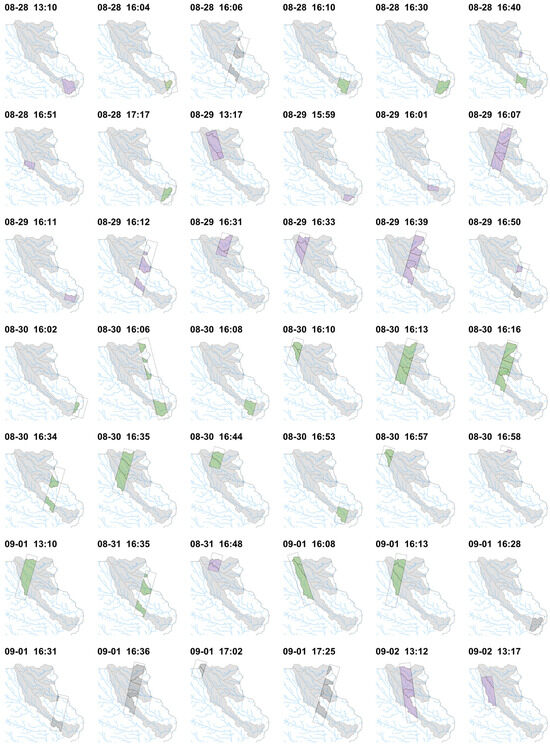
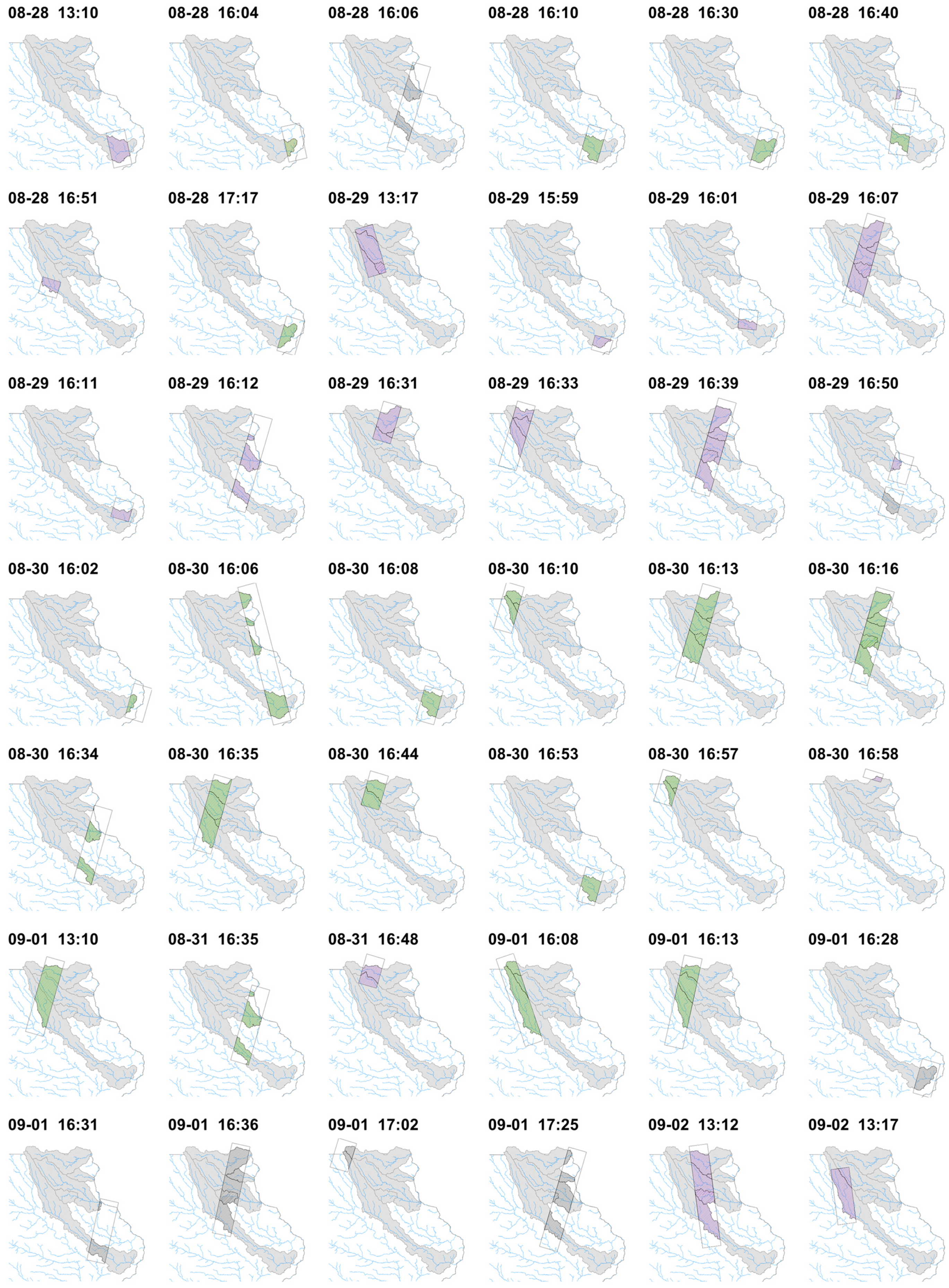
Before presenting examples of flood inundation simulations generated by the hydraulic models and comparing them to satellite-based maps, let us first examine the available satellite imagery for the north-east Iowa flood. Figure 9 presents all available Planet images for the specified period, categorized into four classes: clear, partly cloudy, cloudy, and unavailable. However, due to the limited spatial extent of each image along the ground track, their intersection with the basin boundaries yields a fragmented and incomplete representation of the flood event, hindering a comprehensive analysis.
Figure 9.
PlanetScope scenes available from 08-28 to 08-30, 2021 (time in UTC). Shading indicates images were: clear (green), partially cloudy (dark gray), cloudy (magenta), and not available (gray).
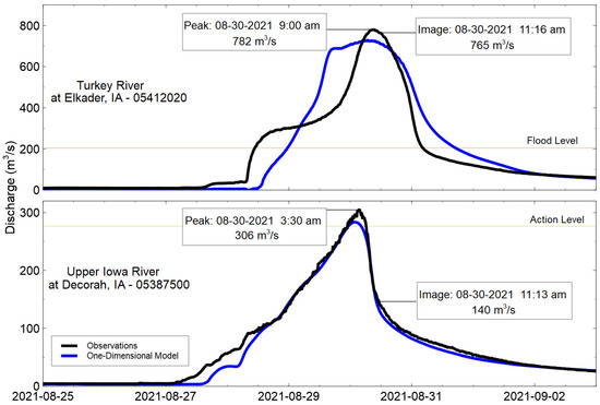
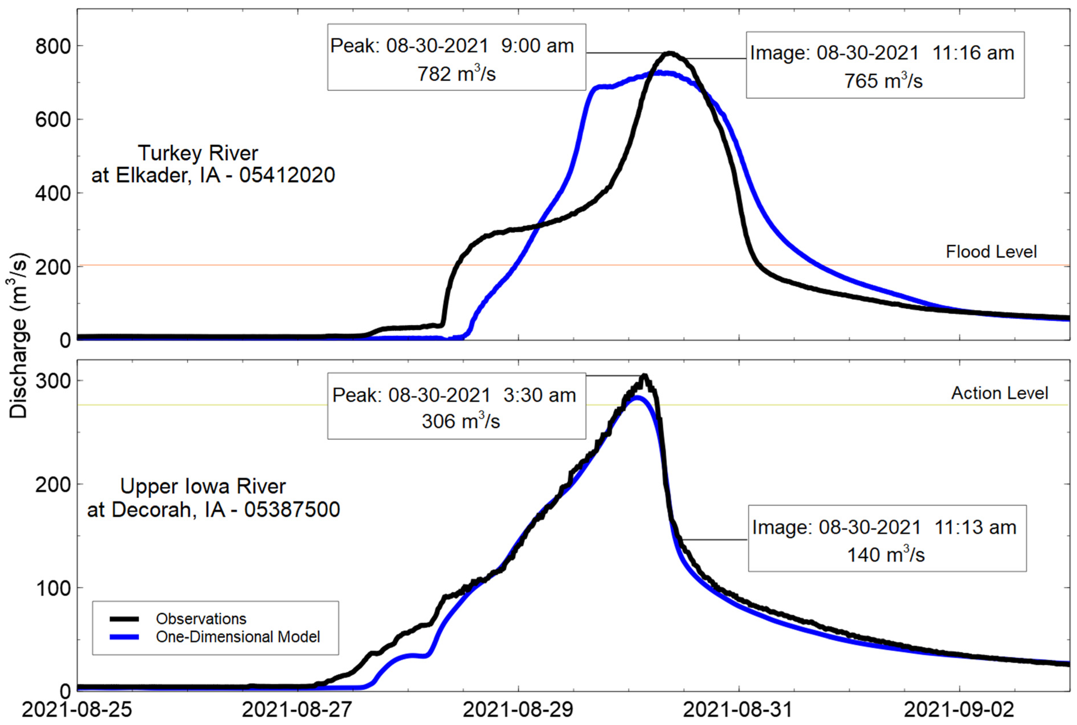
As a result, as seen in the time domain at selected sites (Figure 10), satellites observed the flood peak only at Elkader, after the flood wave has already propagated across the basin, causing damage and hardship. The black line in the panels is the streamflow observation and the blue line is the streamflow simulated with the one-dimensional open channel flow model. The simulated peak flow was reached on 30 August at 06:45 AM, 135 min earlier than the observations where the peak was reached on 30 August, at 09:00 AM. The simulated peak value was 732 m3/s, very close to the observed value of 782 m3/s. According to the simulation, the stage’s highest value of 6.7 m was also reached on 30 August at 06:45 AM, while the highest observed stage of 7.0 m was reached on 30 August at 09:00 AM. Figure 10 also indicates the discharge value at the time of the satellite image was 765 m3/s; the stage at that time was 6.9 m. The differences in timing between simulated and observed data can be because of the resistance values used in the simulation for the main channel. We chose a value of Manning’s n = 0.035 for the entire channel based on experience at neighboring basins and field work; this is a typical roughness value for a riverbed of this type of basin in Iowa, but using a single value might not be representative of the heterogenous roughness conditions in the channel. The performance of the model is also affected by errors in the channel geometry (bathymetry), which is limited using LiDAR topography in the absence of geodetic channel surveys; LiDAR cannot penetrate through water, leading to errors in the location of the bottom of the channel. For the cross-sections corresponding to Elkader, we performed a channel bottom correction based on USGS observations; however, the same procedure is not possible for cross-sections where no survey or observational data is available. The difference between total flow volumes is around 8% at the Elkader location and 2% at the most downstream point of the basin (Garber), which seems acceptable for simulations and gives credibility to the one-dimensional model skill.
Figure 10.
Hydrographs of observed and one-dimensional model-simulated discharge at selected locations. Times when satellite images are available are indicated, along with the corresponding discharge.
We did a similar analysis for the routing of the flood wave at the Upper Iowa River. The plots in Figure 10 show results obtained at the stream gage in Decorah. The simulated peak was 283 m3/s, reached on 30 August at 01:45 AM, 105 min earlier than the observed peak 306 m3/s on August 30 at 03:30 AM. The maximum simulated gage height was 3.1 m while the observed was 2.8 m. For the vicinity of Decorah, the satellite image was taken after the flood peak; in fact, the discharge at that time was 140 m3/s and the stage was 1.9 m, considerably below the observed flood peak.
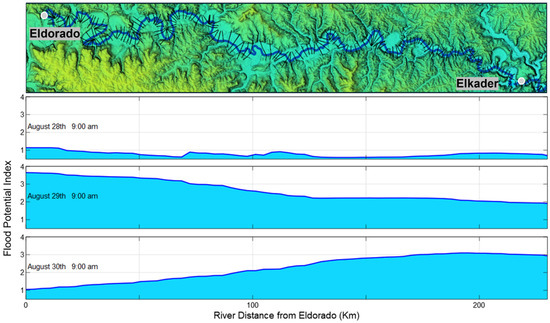
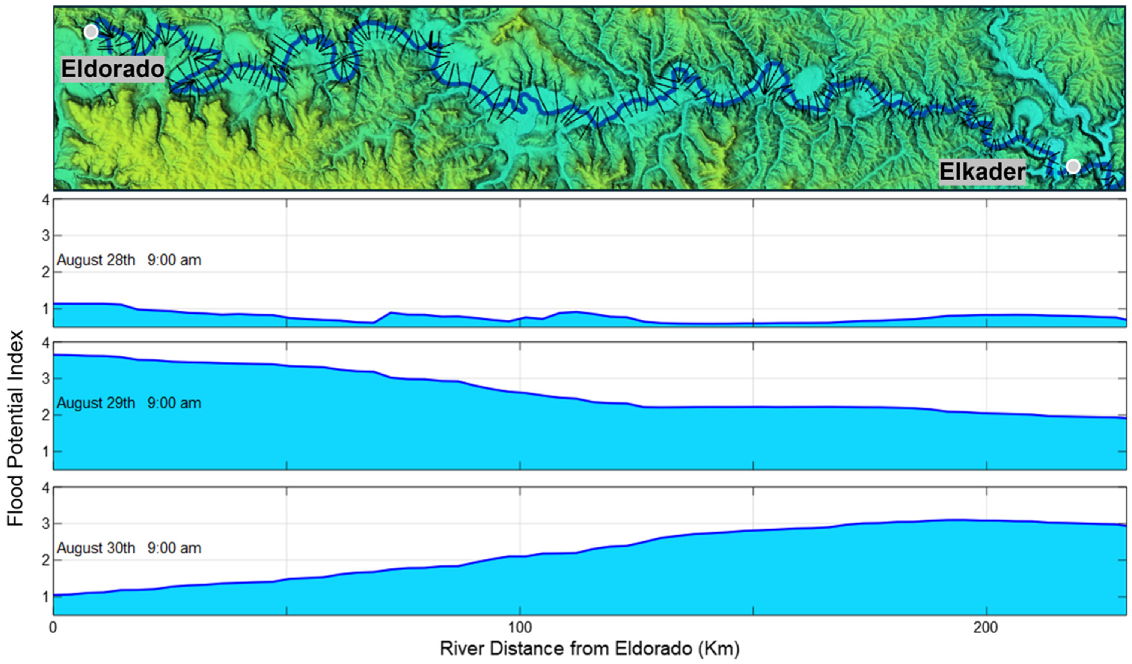
The fortunate coincidence of the flood peak at Elkader and the satellite image is also evident in the results of the one-dimensional model and the routing of the flood wave along the river, between Eldorado and Elkader, about 235 km along the main channel. Figure 11 compares one-dimensional unsteady-state simulations of streamflow at three instances of time, one day apart. The flow is normalized by the mean annual peak, roughly corresponding to bank full flow. Therefore, the values greater than one imply flooding conditions.
Figure 11.
Simulation results of the flood wave propagation along a stretch of the Turkey River over three days. The image above shows the terrain topography, river channel and the cross-sections used in the setup of the one-dimensional model. The plotted quantity is simulation discharge converted to Flood Potential Index. The value of 1 corresponds approximately to bank full flow.
We have also performed a simulation of the flood wave propagation on the Turkey and Upper Iowa rivers using the two-dimensional open channel flow model. The results were very similar to those obtained using the one-dimensional model. We think that this is because we used the same channel hydraulic geometry based on LiDAR topography as well as boundary and initial conditions. As the one-dimensional model is computationally faster and easier to implement in an operational setting, we limit further discussion to the one-dimensional model.
3.4. Satellite-Based and Modeled Inundation Maps
The inundation extension can be extracted from the satellite images. We performed image categorization using the semi-automatic classification plug-in of QGIS [40]. This supervised classification consists of three steps: (1) creating training regions of interest (ROIs) to define flooded and non-flooded areas representative of the entire image; (2) generating a signature list that holds all the defined ROIs; and (3) categorizing the images using the Minimum Distance Algorithm. After creating training cases, we performed the classification of the images available from the two selected sites, obtaining flooded and non-flooded areas. There are some cases where the satellite data show a gap because, when the satellite passes by taking the images, they do not overlap, leaving areas uncovered. These areas were excluded from our classification and labeled as “No data”.
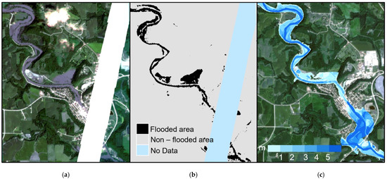
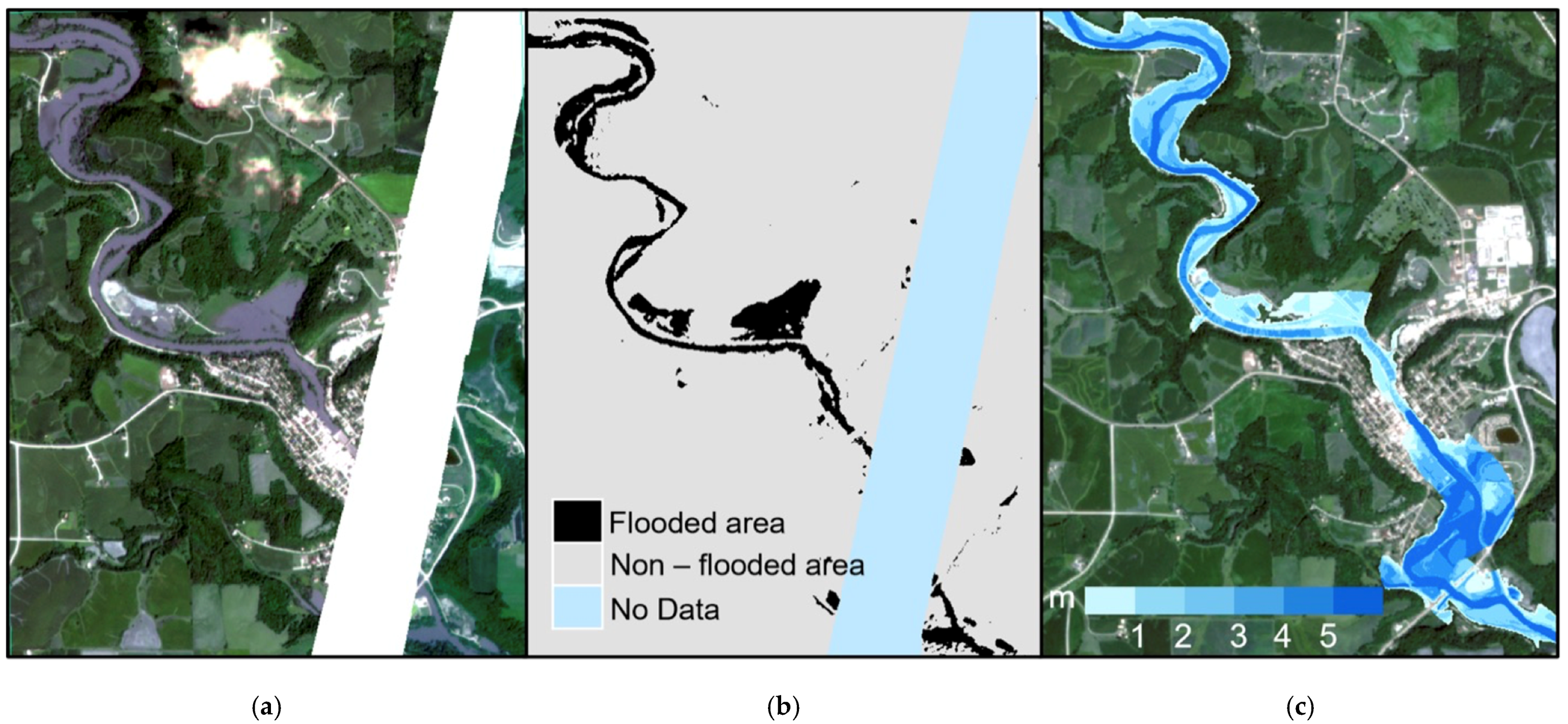
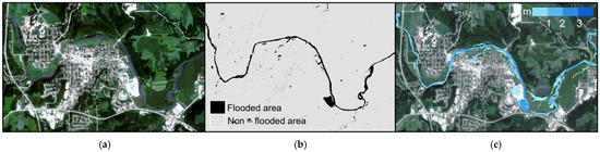
Based on the PlanetScope satellite image’s supervised image classification, we obtained a digital delineation of the flooded and non-flooded areas. Figure 12a shows the image available for the Turkey River at Elkader on 30 August at 16:16 UTC (11:16 AM local time). However, due to the lack of overlap in the satellite images, both figures exhibit a gap, leaving an uncovered area. The classified images, presented in Figure 12b and Figure 13b, identify flooded and non-flooded areas, with the area lacking information classified as “No Data”. These satellite-based inundation maps serve as reference for comparison with modeled flood extent maps described below.
Figure 12.
(a) Original image from PlanetScope for the vicinity of Elkader; (b) the same image classified; and (c) inundation simulated for the same scene by the one-dimensional model (water depth is shown).
Figure 13.
(a) Original image from PlanetScope for the vicinity of Decorah; (b) the same image classified; and (c) inundation simulated for the same scene by the one-dimensional model (water depth is shown).
The flood inundation maps obtained with the one-dimensional models are shown in Figure 12c and Figure 13c, respectively, for Elkader and Decorah. The simulated flood inundation maps for Elkader and Decorah correspond to the dates and times of the available satellite-based inundation maps. Figure 12a shows a clear example of the operational limitations of satellite imagery, where a band of missing data crosses the urban area of Elkader. The hydrologic and hydraulic modeling of the river (Figure 12c) allows us to estimate the extent of the flooding in the area that was not visible to the satellite. Additionally, the hydraulic modeling allows us to estimate the depth of water, providing valuable information to emergency managers on how to prioritize their actions. Forecasting flood extent and depths is possible, but subject to high uncertainty from rainfall forecasts as shown in Figure 7 and Figure 8, and from the parameterization of hydraulic models. This case demonstrates that it is not complementary but crucial to obtain supporting information from both remote sensing and hydrologic/hydraulic modeling approaches during the development of flood events.
4. Discussion and Conclusions
This paper demonstrates the limitations of satellite-based inundation maps for operational forecasting of common floods, emphasizing that flood modeling is not merely a complement to remote sensing estimation, but a crucial component of adequate flood risk assessment. Our findings are in agreement with the scientific literature reporting limitations [28,29,30,31]. The complex dynamics of space–time processes that drive flooding require a multifaceted approach, incorporating resources such as radar-based rainfall observation, numerical weather prediction models, and hydrologic models that convert rainfall to runoff. Notably, these resources also rely heavily on remote sensing, including weather radar for sensing the atmosphere, airborne LiDAR technology for topography data acquisition, and satellite-based monitoring of land use and land cover, all of which play a critical role in streamflow forecasting systems.
Our case study of the northeastern Iowa flood event of August 2021 illustrates the value of these tools in predicting the occurrence and severity of flooding, days in advance before satellites provided useful information. Only at one key location did satellite information coincide with the peak of the flood while useful images were either unavailable or arrived too late at other locations.
Furthermore, high-resolution satellite images are often hindered by cloud cover obstructions, which can persist for extended periods after flood-causing storms have passed. Satellite-based technologies capable of penetrating cloud cover typically have a reduced spatial and temporal resolution, with even a 10–30 m resolution being too coarse for medium-sized basins like the Turkey and Upper Iowa.
In this paper, we present a current, operational viewpoint. Clearly, future advances in remote sensing technologies will allow for the combination of multiple observations with models to enhance predictive skill including the real-time forecasting of floods. For example, satellite data can be used in validating open channel flow models and thus, indirectly contribute to improving forecasting skill (e.g., ref. [41,42]).
Author Contributions
Conceptualization, W.F.K. and E.N.; methodology, E.N., W.F.K., M.R. and F.Q.; validation, M.R. and F.Q.; writing—original draft preparation, M.R. and W.F.K.; writing—review and editing, all authors; supervision, W.F.K. All authors have read and agreed to the published version of the manuscript.
Funding
F.Q was supported by the Cooperative Institute for Research to Operations in Hydrology (CIROH) with funding under award NA22NWS4320003 from the NOAA Cooperative Institute Program. The statements, findings, conclusions, and recommendations are those of the authors and do not necessarily reflect the opinions of NOAA. W.F.K was partially supported by the Rose & Joseph Summers Chair in Water Resources Engineering endowment at the University of Iowa.
Data Availability Statement
All the datasets produced for this paper are available by contacting the Iowa Flood Center. Hydrometeorological data used to force the models is publicly available from the sources listed in the manuscript.
Acknowledgments
E.N. acknowledges participation in project: “Accelerate the Exploitation of Satellite Observations to Improve Flooding and Inundation Monitoring and Forecasts”, supported by NOAA, which was the inspiration for this study.
Conflicts of Interest
The authors declare no conflicts of interest.
Appendix A
Description of Satellite Products
PlanetScope is a product of the company Planet derived from a constellation of approximately 130 satellites able to view the entire land surface of the Earth (200 million km2/day) every day. PlanetScope images have a resolution of approximately three meters per pixel. A PlanetScope Scene Product is a single captured frame within a continuous strip of imagery taken by the satellite as it scans the Earth, with each scene covering between 280 and 630 square kilometers depending on the specific instrument used to capture it. They are represented in the Planet Platform as PSScene item types. PSScene supports access to 8-band imagery (RGB, NIR, Red Edge, Yellow, Green I, and Coastal Blue).
SENTINEL-2 (L1C and L2A) are products of the European wide-swath, high-resolution, multi-spectral imaging mission. Its high-resolution optical images have many applications, including land monitoring, emergency response and security services assistance. The satellite’s multi-spectral imager provides a versatile set of 13 spectral bands spanning from the visible and near-infrared to the shortwave infrared. The spatial resolution is 10 m, 20 m, and 60 m depending on the wavelength. Revisit time is five days with two satellites and 10 days for a single satellite. The SENTINEL-2 images available for the selected sites and analyzed dates are, unfortunately, low-resolution (10 m and 20 m spatial resolution) and contain clouds that hinder visibility.
The Operational Land Imager (OLI) and Thermal Infrared Sensor (TIRS) onboard the Landsat 8 satellite have acquired images of the Earth since February 2013. Each sensor collects images of the Earth with a 16-day repeat cycle, referenced to the Worldwide Reference System-2. Each satellite collects data on an eight-day offset. The approximate scene size is 170 km north–south by 183 km east–west (106 mi by 114 mi). Landsat 8–9 image data files consist of 11 spectral bands with a spatial resolution of 30 m for bands 1–7 and bands 9–11, and 15 m for the panchromatic band 8. The products were not used for our study due to the low resolution of these images.
SkySat is a high-resolution product of the company Planet with a constellation of 21 satellites able to revisit any location on Earth up to ten times per day with a daily collection capacity of 400,000 km2/day. SkySat images are approximately 50 cm per pixel resolution. The SkySat satellite constellation consists of multiple launches of the SkySat-C generation satellites, first launched in 2016. Each satellite is three-axis-stabilized and agile enough to slew between different targets of interest. Each satellite has four thrusters for orbital control, along with four reaction wheels and three magnetic torquers for attitude control. All SkySats contain Cassegrain telescopes with a focal length of 3.6 m, with three 5.5-megapixel CMOS imaging detectors making up the focal plane. A SkySat Scene Product is an individual framed scene within a strip, captured by the satellite in its line-scan of the Earth. SkySat Satellites have three cameras per satellite, which capture three overlapping strips. Each of these strips contain overlapping scenes, not organized to any particular tiling grid system. SkySat Scene products are approximately 2.5 km2 in size. These images should be ordered in advance and must specify the exact day or, at most, a two-week window for the required image. Unfortunately, there were no SkySat images available in the records for any of the study locations within the specified date range, so we were unable to obtain them for this study.
References
- Notti, D.; Giordan, D.; Caló, F.; Pepe, A.; Zucca, F.; Galve, J.P.; Notti, D.; Giordan, D.; Caló, F.; Pepe, A.; et al. Potential and Limitations of Open Satellite Data for Flood Mapping. Remote Sens. 2018, 10, 1673. [Google Scholar] [CrossRef] [Scilit]
- Johnson, J.M.; Munasinghe, D.; Eyelade, D.; Cohen, S. An Integrated Evaluation of the National Water Model (NWM)–Height Above Nearest Drainage (HAND) Flood Mapping Methodology. Nat. Hazards Earth Syst. Sci. 2019, 19, 2405–2420. [Google Scholar] [CrossRef] [Scilit]
- Krajewski, W.F.; Ceynar, D.; Demir, I.; Goska, R.; Kruger, A.; Langel, C.; Mantilla, R.; Niemeier, J.; Quintero, F.; Seo, B.C.; et al. Real-Time Flood Forecasting and Information System for the State of Iowa. Bull. Am. Meteorol. Soc. 2017, 98, 539–554. [Google Scholar] [CrossRef] [Scilit]
- Mantilla, R.; Krajewski, W.F.; Velasquez, N.; Small, S.J.; Ayalew, T.B.; Quintero, F.; Jadidoleslam, N.; Fonley, M. The Hydrological Hillslope-Link Model for Space-Time Prediction of Streamflow: Insights and Applications at the Iowa Flood Center. In Extreme Weather Forecasting; Astitha, M., Nikolopoulos, E.I., Eds.; Elsevier: Amsterdam, The Netherlands, 2022; ISBN 978-0-12-820124-4. [Google Scholar]
- Gilles, D.; Young, N.; Schroeder, H.; Piotrowski, J.; Chang, Y.J. Inundation Mapping Initiatives of the Iowa Flood Center: Statewide Coverage and Detailed Urban Flooding Analysis. Water 2012, 4, 85–106. [Google Scholar] [CrossRef] [Scilit]
- Zhang, J.; Howard, K.; Langston, C.; Kaney, B.; Qi, Y.; Tang, L.; Grams, H.; Wang, Y.; Cockcks, S.; Martinaitis, S.; et al. Multi-Radar Multi-Sensor (MRMS) Quantitative Precipitation Estimation: Initial Operating Capabilities. Bull. Am. Meteorol. Soc. 2016, 97, 621–638. [Google Scholar] [CrossRef] [Scilit]
- Benjamin, S.G.; Weygandt, S.S.; Brown, J.M.; Hu, M.; Alexander, C.R.; Smirnova, T.G.; Olson, J.B.; James, E.P.; Dowell, D.C.; Grell, G.A.; et al. A North American Hourly Assimilation and Model Forecast Cycle: The Rapid Refresh. Mon. Weather. Rev. 2016, 144, 1669–1694. [Google Scholar] [CrossRef] [Scilit]
- James, E.P.; Alexander, C.R.; Dowell, D.C.; Weygandt, S.S.; Benjamin, S.G.; Manikin, G.S.; Brown, J.M.; Olson, J.B.; Hu, M.; Smirnova, T.G.; et al. The High-Resolution Rapid Refresh (HRRR): An Hourly Updating Convection-Allowing Forecast Model. Part II: Forecast Performance. Weather Forecast. 2022, 37, 1397–1417. [Google Scholar] [CrossRef] [Scilit]
- Cosgrove, B.; Gochis, D.; Flowers, T.; Dugger, A.; Ogden, F.; Graziano, T.; Clark, E.; Cabell, R.; Casiday, N.; Cui, Z.; et al. NOAA’s National Water Model: Advancing Operational Hydrology through Continental-Scale Modeling. JAWRA J. Am. Water Resour. Assoc. 2024, 60, 247–272. [Google Scholar] [CrossRef] [Scilit]
- Roux, H.; Amengual, A.; Romero, R.; Bladé, E.; Sanz-Ramos, M. Evaluation of Two Hydrometeorological Ensemble Strategies for Flash-Flood Forecasting over a Catchment of the Eastern Pyrenees. Nat. Hazards Earth Syst. Sci. 2020, 20, 425–450. [Google Scholar] [CrossRef] [Scilit]
- Awol, F.S.; Coulibaly, P.; Tsanis, I. Identification of Combined Hydrological Models and Numerical Weather Predictions for Enhanced Flood Forecasting in a Semiurban Watershed. J. Hydrol. Eng. 2021, 26, 04020057. [Google Scholar] [CrossRef] [Scilit]
- Trošelj, J.; Nayak, S.; Hobohm, L.; Takemi, T. Real-Time Flash Flood Forecasting Approach for Development of Early Warning Systems: Integrated Hydrological and Meteorological Application. Geomat. Nat. Hazards Risk 2023, 14, 2269295. [Google Scholar] [CrossRef] [Scilit]
- Saleh, F.; Ramaswamy, V.; Georgas, N.; Blumberg, A.F.; Pullen, J. A Retrospective Streamflow Ensemble Forecast for an Extreme Hydrologic Event: A Case Study of Hurricane Irene and on the Hudson River Basin. Hydrol. Earth Syst. Sci. 2016, 20, 2649–2667. [Google Scholar] [CrossRef] [Scilit]
- Sayama, T.; Yamada, M.; Sugawara, Y.; Yamazaki, D. Ensemble Flash Flood Predictions Using a High-Resolution Nationwide Distributed Rainfall-Runoff Model: Case Study of the Heavy Rain Event of July 2018 and Typhoon Hagibis in 2019. Prog. Earth Planet. Sci. 2020, 7, 75. [Google Scholar] [CrossRef] [Scilit]
- Bacelar, L.; ReifeeiNasab, A.; Chaney, N.; Barros, A. Barriers to Operational Flood Forecasting in Complex Terrain: From Precipitation Forecasts to Probabilistic Flood Forecast Mapping at Short Lead Times. Preprints 2023. [Google Scholar] [CrossRef] [Scilit]
- Cifelli, R.; Chandrasekar, V.; Herdman, L.; Turner, D.D.; White, A.B.; Alcott, T.I.; Anderson, M.; Barnard, P.; Biswas, S.K.; Boucher, M.; et al. Advanced Quantitative Precipitation Information: Improving Monitoring and Forecasts of Precipitation, Streamflow, and Coastal Flooding in the San Francisco Bay Area. Bull. Am. Meteorol. Soc. 2024, 105, E313–E331. [Google Scholar] [CrossRef] [Scilit]
- Huang, J.-K.; Chan, Y.-H.; Lee, K.T. Real-Time Flood Forecasting System: Case Study of Hsia-Yun Watershed, Taiwan. J. Hydrol. Eng. 2016, 21, 05015031. [Google Scholar] [CrossRef] [Scilit]
- Brendel, C.E.; Dymond, R.L.; Aguilar, M.F. Integration of Quantitative Precipitation Forecasts with Real-Time Hydrology and Hydraulics Modeling towards Probabilistic Forecasting of Urban Flooding. Environ. Model. Softw. 2020, 134, 104864. [Google Scholar] [CrossRef] [Scilit]
- Ivanov, V.Y.; Xu, D.; Dwelle, M.C.; Sargsyan, K.; Wright, D.B.; Katopodes, N.; Kim, J.; Tran, V.N.; Warnock, A.; Fatichi, S.; et al. Breaking Down the Computational Barriers to Real-Time Urban Flood Forecasting. Geophys. Res. Lett. 2021, 48, e2021GL093585. [Google Scholar] [CrossRef] [Scilit]
- Coelho, G.D.A.; Ferreira, C.M.; Kinter, J.L., III. Multiscale and Multi Event Evaluation of Short-Range Real-Time Flood Forecasting in Large Metropolitan Areas. J. Hydrol. 2022, 612, 128212. [Google Scholar] [CrossRef] [Scilit]
- Diaz, F.J.G.; Jafarzadegan, K.; Moftakhari, H.; Moradkhani, H. Accounting for the Uncertainty of Precipitation Forecasts and Its Impacts on Probabilistic Flood Inundation Mapping Skill. Preprints 2025. [Google Scholar] [CrossRef] [Scilit]
- Huang, Z.; Wu, H.; Gu, G.; Li, X.; Nanding, N.; Adler, R.F.; Yilmaz, K.K.; Alfieri, L.; Chen, S. Paired Satellite and NWP Precipitation for Global Flood Forecasting. J. Hydrometeorol. 2023, 24, 2191–2205. [Google Scholar] [CrossRef] [Scilit]
- Pagano, T.C. Evaluation of Mekong River Commission Operational Flood Forecasts, 2000–2012. Hydrol. Earth Syst. Sci. 2014, 18, 2645–2656. [Google Scholar] [CrossRef] [Scilit]
- Post, R.; Quintero, F.; Krajewski, W.F. Forecast-Informed Reservoir Operation within an Actively Managed Distributed Storage Network Using the High-Resolution Rapid Refresh Product. J. Water Resour. Plan. Manag. 2025, 151, 04024065. [Google Scholar] [CrossRef] [Scilit]
- Seo, B.-C.; Quintero, F.; Krajewski, W.F. High-Resolution QPF Uncertainty and Its Implications for Flood Prediction: A Case Study for the Eastern Iowa Flood of 2016. J. Hydrometeorol. 2018, 19, 1289–1304. [Google Scholar] [CrossRef] [Scilit]
- Vergara, H.; Gourley, J.J.; Erickson, M. An Efficient Ensemble Technique for Hydrologic Forecasting Driven by Quantitative Precipitation Forecasts. J. Hydrometeorol. 2023, 24, 479–495. [Google Scholar] [CrossRef] [Scilit]
- Viterbo, F.; Mahoney, K.; Read, L.; Salas, F.; Bates, B.; Elliott, J.; Cosgrove, B.; Dugger, A.; Gochis, D.; Cifelli, R. A Multiscale, Hydrometeorological Forecast Evaluation of National Water Model Forecasts of the May 2018 Ellicott City, Maryland, Flood. J. Hydrometeorol. 2020, 21, 475–499. [Google Scholar] [CrossRef] [Scilit]
- Revilla-Romero, B.; Beck, H.E.; Burek, P.; Salamon, P.; De Roo, A.; Thielen, J. Filling the Gaps: Calibrating a Rainfall-Runoff Model Using Satellite-Derived Surface Water Extent. Remote Sens. Environ. 2015, 171, 118–131. [Google Scholar] [CrossRef] [Scilit]
- Revilla-Romero, B.; Hirpa, F.A.; Pozo, J.T.; Salamon, P.; Brakenridge, R.; Pappenberger, F.; De Groeve, T. On the Use of Global Flood Forecasts and Satellite-Derived Inundation Maps for Flood Monitoring in Data-Sparse Regions. Remote Sens. 2015, 7, 15702–15728. [Google Scholar] [CrossRef] [Scilit]
- Yilmaz, K.K.; Adler, R.F.; Tian, Y.; Hong, Y.; Pierce, H.F. Evaluation of a Satellite-Based Global Flood Monitoring System. Int. J. Remote Sens. 2010, 31, 3763–3782. [Google Scholar] [CrossRef] [Scilit]
- Schumann, G.; Giustarini, L.; Tarpanelli, A.; Jarihani, B.; Martinis, S. Flood Modeling and Prediction Using Earth Observation Data. Surv. Geophys. 2023, 44, 1553–1578. [Google Scholar] [CrossRef] [Scilit]
- Mason, D.C.; Bevington, J.; Dance, S.L.; Revilla-Romero, B.; Smith, R.; Vetra-Carvalho, S.; Cloke, H.L. Improving Urban Flood Mapping by Merging Synthetic Aperture Radar-Derived Flood Footprints with Flood Hazard Maps. Water 2021, 13, 1577. [Google Scholar] [CrossRef] [Scilit]
- Gerard, A.; Martinaitis, S.M.; Gourley, J.J.; Howard, K.W.; Zhang, J. An Overview of the Performance and Operational Applications of the MRMS and FLASH Systems in Recent Significant Urban Flash Flood Events. Bull. Am. Meteorol. Soc. 2021, 102, E2165–E2176. [Google Scholar] [CrossRef] [Scilit]
- Running, S.; Mu, Q.; Zhao, M.; Moreno, A. MODIS/Terra Net Evapotranspiration 8-Day L4 Global 500m SIN Grid V061. NASA EOSDIS Land Processes DAAC 2021, 1.5, 34. [Google Scholar]
- Brunner, G. HEC-RAS River Analysis System, Hydraulic Reference Manual, Version 4.1; US Army Corps of Engineers Hydrologic Engineering Center: Davis, CA, USA, 2010; pp. 1–790.
- Chow, V.T. Open-Channel Hydraulics. In Open-Channel Hydraulics; McGraw-Hill: Columbus, OH, USA, 1959. [Google Scholar]
- Brunner, G.W.; Warner, J.C.; Wolfe, B.C.; Piper, S.S.; Marston, L. HEC-RAS, River Analysis System. Applications Guide; US Army Corps of Engineers Hydrologic Engineering Center: Davis, CA, USA, 2016; p. 150.
- Krajewski, W.F.; Goska, R.; Post, R.; Quintero, F.; Velasquez, N. Is This Rainfall Forecast Good or Bad? For Flood Forecasting, the Answer Is Scale Dependent. Bull. Am. Meteorol. Soc. 2025, 106, E1772–E1793. [Google Scholar] [CrossRef] [Scilit]
- Ghimire, G.R.; Krajewski, W.F.; Ayalew, T.B.; Goska, R. Hydrologic Investigations of Radar-Rainfall Error Propagation to Rainfall-Runoff Model Hydrographs. Adv. Water Resour. 2022, 161, 104145. [Google Scholar] [CrossRef] [Scilit]
- Congedo, L. Semi-Automatic Classification Plugin: A Python Tool for the Download and Processing of Remote Sensing Images in QGIS. J. Open Source Softw. 2021, 6, 3172. [Google Scholar] [CrossRef] [Scilit]
- Horritt, M.S. Calibration of a Two-Dimensional Finite Element Flood Flow Model Using Satellite Radar Imagery. Water Resour. Res. 2000, 36, 3279–3291. [Google Scholar] [CrossRef] [Scilit]
- Masafu, C.; Williams, R. Satellite Video Remote Sensing for Flood Model Validation. Water Resour. Res. 2024, 60, e2023WR034545. [Google Scholar] [CrossRef] [Scilit]
Disclaimer/Publisher’s Note: The statements, opinions and data contained in all publications are solely those of the individual author(s) and contributor(s) and not of MDPI and/or the editor(s). MDPI and/or the editor(s) disclaim responsibility for any injury to people or property resulting from any ideas, methods, instructions or products referred to in the content. |
© 2026 by the authors. Licensee MDPI, Basel, Switzerland. This article is an open access article distributed under the terms and conditions of the Creative Commons Attribution (CC BY) license.