


Abstract
Driving rain or ‘wind-driven rain’ (WDR) arrives at the ground on an oblique trajectory, and drops may strike at a speed greater than their still-air terminal velocity. Oblique rain can affect a range of geomorphic processes including the splash dislodgment and transport of soil particles, and hydrological processes including overland flow, canopy interception, and the generation of stemflow. The mean rain inclination angle at which WDR strikes the ground has been estimated from the catch of paired gauges, one with a conventional horizontal orifice, and one with a vertical orifice, or by related forms of vectopluviometers. Such data allow the resolution of rain vectors to find the rain inclination. However, rain-collecting devices of this kind do not permit the real-time recording of the rain inclination from moment to moment. Here, a new acoustic method for measuring the rain inclination is introduced that provides an inexpensive tool for the continuous, real-time monitoring of WDR. Furthermore, the method also permits the simultaneous recording of rainfall duration and intermittency at a high temporal resolution, with no additional apparatus. Data on rain inclinations collected during showers on a tropical coast exposed to strong trade-winds are presented to illustrate the operation of the acoustic measurement system. However, the focus of this paper is the presentation of the new method itself, and not on the climatology of WDR.
1. Introduction
Rain is frequently accompanied by wind, and, indeed, it has been argued that “wind-driven rain is the primary form of natural rainfall.” (An et al. 2022, p. 2) [1]. This ‘wind-driven rain’ (hereafter referred to as WDR) typically exhibits drop trajectories that are not vertical, as seen in still air, but which approach the ground obliquely. Whilst wind and rain are recorded as separate parameters at meteorological ground stations, their combined influence on rain droplet trajectories is not usually recorded or analysed. Likewise, the angle of inclination of WDR is not routinely recorded, despite its significance, which is considered further below. This is likely to reflect the lack of a suitable apparatus for recording the angle at which droplets following oblique trajectories strike the ground. A solution to this is introduced in the present work.
In the context of fields including geomorphology, pedology, and hydrology, two key attributes of WDR are the angle (or inclination) of oblique arrival of drops deflected by the wind, and the potentially greater impact velocity and droplet kinetic energy conferred by the wind acceleration of the droplets. In WDR, drop speeds can exceed their still-air terminal fall velocity. Particularly if the wind vector at the ground surface is directed broadly in the upslope direction, upslope splash transport and particle creep may exceed downslope transport, and surface runoff may be slowed by the upslope wind and droplet-impact drag. The reverse may occur with downslope-directed WDR. Infiltration and sediment transport in overland flow can both also be affected. Additional details are provided in Section 1.2. Before introducing the new apparatus for recording the rain inclination, we begin with some necessary additional background to the characteristics of WDR.
1.1. A Note on Terminology
In the remainder of this paper, the expression ‘wind-driven rain’ (WDR) is used as a general term to refer to rain in which drops fall toward the ground at an angle, rather than vertically, and in which the speed of the fall of the droplets may not correspond with the expected still-air terminal velocity. ‘Rain inclination’ is used here to refer to the angle of arrival of rain at the ground, measured from the horizontal. When rain driven by wind is referred to, it may be referred to as ‘oblique rain’, drawing specific attention to the rain inclination resulting from wind. Where individual droplets are being referred to, reference is made to their ‘trajectory’—the path that droplets follow in their approach to the ground.
1.2. The Behaviour of Rainfall Affected by Wind
Given that terminal raindrop fall speeds in still air are <10 m s−1 even for very large drops of 5 mm diameter (Gunn and Kinzer 1949) [2], horizontal wind speed can easily exceed the droplet fall speed. A wind speed of 10 m s−1 only reaches the ‘fresh breeze’ category in the Beaufort scale. The ‘strong breeze’ class extends to 13.6 m s−1, and ‘gale’ extends to >20 m s−1. Tropical cyclones traversing Queensland, Australia are frequently associated with heavy rainfall and large total depths. Direct observation has shown that peak 10-min wind speeds can exceed 50 m s−1 (O’Grady et al. 2024) [3]. Clearly, wind speeds can greatly exceed the terminal velocity of even the largest drops, such that drops can strike the ground surface or vegetation not only obliquely but also at considerable speed.
This can be understood from the finding that horizontal speeds of droplets deflected by wind tend broadly to match the wind speed (Fu et al. 2015 [4], Lu et al. 2019 [5]), with scatter in the relationship to be expected as a result of wind gustiness, turbulence, and the drop size distribution (DSD). Departures of the droplet speed from the wind speed can occur because the wind speeds may be lower close to the ground than at higher elevations where the surface frictional drag is less. As a result of their inertia, larger droplets falling toward the ground from areas of higher wind speed aloft may have a horizontal speed that exceeds the wind speed close to the ground (Fu et al. 2015 [4]), and will be deflected less by the wind. Nevertheless, the speeds of droplets of up to 5 mm diameter can track fluctuating wind speeds quite rapidly, over just seconds, though smaller drops respond more rapidly than do larger ones (refer to data presented in Figure 5 in Fu et al. 2015 [4]).
Under steady, unidirectional wind, and assuming that the drop velocity matches the wind speed fairly closely, the angle of inclination of the drop trajectories toward the ground (usually expressed in terms of the angle of departure from the vertical) can be estimated as the vector sum of the wind speed (v, m s−1) and the fall speed of a droplet (normally taken as the still-air fall speed, u, m s−1). Thus, the angle of inclination from the vertical is given by
The trajectory of a droplet having a terminal velocity of 6.5 m s−1 in a wind of 1.5 m s−1 would thus nominally be inclined at ~13° from the vertical. Van Heerden (1961) [6] argued for the term ‘deviation’ for oblique drop trajectories, to emphasise that it was a departure from the ‘normal’ vertical trajectory. This term appears not to have found common use in the literature, and the angle specified in Equation (1) is referred to here as the inclination of the rain.
Because u can take the same value as v, the inclination of droplet trajectories from the vertical can readily reach 45° or more. For instance, a 1 mm-diameter droplet has a terminal velocity of ~4 m s−1, and reaching = 45° therefore only requires a wind speed of ~4 m s−1 (~14 km h−1). To reach 45° inclination, even a larger 4 mm drop would require a wind speed of only ~9 m s−1 (~32 km h−1) in the Beaufort ‘fresh breeze’ range. Mean monthly 3 pm wind speeds at Cairns, Australia (in the trade winds region where the rain inclination data reported below were collected) lie between 4–5.5 m s−1 (15–20 km h−1) but a significant proportion lie between ~5.5 m s−1–8 m s−1 (20–30 km h−1) (Bureau of Meteorology, Australia, 2025 [7]) Thus, it is to be expected that, during trade wind showers in this region, or in other wind-exposed areas globally, many droplets arrive obliquely at the ground. Belcher et al. (2023) [8] presented a climatology of extreme WDR for the south-eastern USA. They reported that 50-year return period winds concurrent with moderately intense rain of ≥~15 mm h−1 exceeded 45 m s−1. Under those conditions, even a very large drop with a terminal velocity of 10 m s−1 would be deflected more than 77° from the vertical (a very oblique trajectory inclined at just ~13° from level ground). Thus, in areas of the world where there are persistent winds, such as the trade wind belts, WDR must be common and rain inclinations can be very steep indeed.
Figure 1 illustrates the form of the relationship between and wind speed for droplets of 1.5 mm diameter and wind speeds up to 10 m s−1, based on the droplet terminal velocities from Gunn and Kinzer (1949) [2]. This assumes a wind parallel to the ground and that the droplet fall speed is unaffected by the wind. In a wind of 5 m s−1, droplets of this size would evidently be inclined at ~45° from the horizontal. Their fall trajectory would only approach vertical in quite low wind speeds. The relationship in Figure 1 is unlikely to correspond exactly to the droplet behaviour in nature. This is not least because, whilst falling, the larger droplets deform and depart from the spherical form of very small droplets, thereby increasing the drag coefficient through the air (Lu et al. 2019) [5]. Deformation is likely to be reduced for a droplet moving at the same speed as the air, owing to a lack of frictional drag. Thus, it cannot be assumed that droplet fall speeds in windy conditions correspond with still-air values determined experimentally. For instance, Testik and Bolek (2023) [9] reported that, of almost 27,000 drops measured in a study in Texas, USA, 18.5% showed sub-terminal fall speeds, and 9.5% were super-terminal, effects that were related to the influence of wind and turbulence. Drop speeds may also be affected by other microphysical processes, including drop oscillation, that again influence frictional drag effects (Testik and Barros 2007) [10]. Testik and Pei (2017) [11] used the data collected in Okalhoma USA, using video and Parsivel disdrometers, to show that, as the wind speed increased, small droplets became more common and large droplets less common. They concluded that the reduced number of large drops in higher wind speeds was attributable to the collisional breakup of drops. The resulting changes in the DSD with wind speed, especially when the wind speed fluctuates, and linked with the mix of sub- and super-terminal drops (Montero-Martínez and García-García 2016 [12], Testik and Bolek 2023 [9]), make the estimation of DSDs from empirical relationships linking DSD and intensity (e.g., as employed by Herwitz and Slye 1992) [13], or using other empirical relationships that neglect wind and turbulence in order to estimate rain inclinations, considerably less certain. The details of how these effects on droplet behaviour vary with wind speed and other atmospheric conditions, including air density, remain in need of additional study.
Figure 1.
The relationship between inclination and wind speed for droplets of 1.5 mm diameter. The data are derived from the work of Gunn and Kinzer (1949) [2].
Given the range of drop diameters present in rain, it can be reasoned that WDR includes droplets falling at a range of inclinations. The smallest droplets can often be seen blowing almost horizontally. Van Heerden (1961) [6] described the ‘waves of mist’ (comprised of these small droplets) that can be seen passing though oblique rain composed of larger drops. Given the apparatus used, with gauges mounted at multiple angles of tilt (see Plate 1 in Van Heerden 1961 [6]), he indicated that the measurement of the inclination of rainfall could be based on the inclination at which the largest event rain depth is recorded.
1.3. What Effects Arise at the Soil Surface During WDR?
The focus of this paper is on a new measurement technique. However, a brief commentary on the impact of WDR at the land surface is provided to illustrate some important aspects of the geomorphic and hydrologic significance of WDR.
The angle at which the droplets finally strike the ground depends on the gradient of the land surface, and the relative directions of the maximum slope direction and the incident wind azimuth. Hillslopes directly facing the wind would experience smaller effective rain inclinations at the ground, and, on steep slopes facing the wind, WDR could strike orthogonally to the ground. More complex conditions can arise in the landscape, where not only does the hillslope steepness and azimuth of the fall vary, but the wind and WDR can also be steered by interaction with topographic barriers, the orientation of valleys, etc. (Hamilton 1954 [14], Sharon 1980 [15], Mao et al. 2023 [16]). The importance of the exposure to WDR in relation to the landform and geomorphic development has been illustrated from a field study of biancana badlands (Tuscany, Italy, Marsico et al. 2021 [17]), and in relation to rill cutting on spoil heaps (Belgium and France, Beullens et al. 2014 [18]).
Experimental studies of processes including soil splash have established that, in WDR, the kinetic energy of rain can be larger than expected for still air (Pedersen and Hasholt 1995 [19], Helming 2001 [20]); however, as was just noted, the impact at the ground depends on the topography. Thus, slopes facing the wind may experience the increased splash detachment of soil particles, though the speed of the overland flow may be lower owing to the upslope-directed wind (Schmidt et al. 2017 [21], An et al. 2022 [1], 2023 [22]). Slopes inclined away from the wind can experience a reduced droplet impact and rainfall intensity. Rather than being carried out in the field under natural rain and wind, the available studies seeking to understand and quantify splash and sediment transport under WDR have primarily been made in indoor flumes where simulated wind and rain can be generated together using fans and spray nozzles (Lyles et al. 1969 [23], Lyles 1976 [24], Erpul et al. 2003 [25], 2004 [26], An et al. 2022 [1], Kalehhouei et al. 2023 [27], Fidari et al. 2024 [28]). Portable wind and rain facilities have also been used on soil surfaces in the field (Ries et al. 2014 [29], Kuhn et al. 2014 [30]), sometimes with wind erosion and water erosion studied separately, in an attempt to evaluate their relative importance (Marzen et al. 2019 [31]). These studies have contributed to an understanding of the diverse outcomes of WDR at the soil surface, and highlighted the importance of WDR to various surface processes. For instance, Lyles et al. (1969) [23] showed that up to 66% more soil mass was dislodged from clods exposed to rain and wind at 13.4 m s−1 than under rain of the same intensity but without wind. Despite findings such as this, flume studies do not fully capture all important aspects of natural events, where there may be intensity bursts during rainfall, strong wind gusts rather than constant wind speeds (Choi 2001 [32]), and a three-dimensional land surface. Intensity bursts can be critical to particle dislodgement (Dunkerley 2019 [33]), and it is important to recall that, in nature, wind gusts, with attendant changes in rain inclination and raindrop kinetic energy, are likely to be virtually ubiquitous and to add to the local variability of rain impact at the soil surface. Furthermore, as emphasised by Ries et al. (2014) [29], flume studies generally use trays or flumes of repacked soil, with no vegetation or litter cover, and no realistic microtopography, macropores from faunal activity, intact biological soil crusts, intact distributions of pore sizes, or other features relevant to surface processes. Measurements of the splash under natural rainfall, made using splash cups or similar methods to record the particle motion (Pedersen and Hasholt 1995 [19], Zambon et al. 2020 [34]), are less common and have lacked a means to record the changing inclination of rain during storms. In pioneering work on rainfall in hilly terrain, Sharon (1980) [15] pointed out that the rain inclination cannot be regarded as constant under natural storm conditions.
1.4. WDR Is Typically Not Targeted in Field Experiments Using Rainfall Simulation
Experimental studies of hydro-geomorphic processes of infiltration, surface runoff, and sediment entrainment and transport made in the field would ideally be made under natural rainfall (Liu et al. 2022) [35]. However, controlled experimental conditions are often preferred, and frequently rely on a constant-intensity rainfall simulation over small experimental plots. Generally, wind is, out of necessity, excluded through the use of shields and other forms of enclosure (Williams et al. 1998 [36], Humphry et al. 2002 [37], Sangüesa et al. 2010 [38], Lascano et al. 2019 [39], Lazarus et al. 2023 [40]) such that the droplets fall vertically toward the soil surface. This is done in order that the simulated rain is not swept aside to fall partly outside the margins of the experimental plot. However, the exclusion of wind also precludes the documentation of the potentially important role of WDR in surface processes. One of the very few studies that provide direct observational evidence of the role of WDR observed in the field is the work of Vieira et al. (2004) [41] in Portugal. This study used marked tracer particles to document the upslope particle transport under WDR driving in that direction. Clearly, the incorporation of wind effects (and WDR) in field and laboratory rainfall simulation studies would better reflect the conditions commonly found in nature. The laboratory flume studies that have included both the fan-driven wind and rainfall simulation appear to be vastly out-numbered by field and laboratory studies where simulated rain alone is used, with wind exclusions and drops all falling vertically to the ground surface or soil tray. The geomorphic and hydrologic effects of WDR therefore warrant additional study, and this would be most informative if carried out under field conditions where the various microphysical influences on DSD discussed earlier, together with wind gustiness and rain intensity fluctuations, would automatically be incorporated. The limited attention to WDR in areas such as soil erosion is reflected in the published literature, as a few examples will show. In their analyses of raindrop impact and interrill erosion, Nouhou Bako et al. (2016 [42], 2017 [43]) did not mention wind, only considering vertical drop impacts. A review of rainfall, erosion, and sediment transport (Giráldez et al. 2022 [44]) includes only a single paragraph on wind effects. A discussion of global rainfall erosivity scenarios for 2050 and 2070 (Panagos et al. 2022 [45]) does not mention wind or WDR at all, despite the evident importance of WDR and the documented secular changes in global wind speeds (Zeng et al. 2019 [46], Zha et al. 2021 [47]) and related changes in DSDs and kinetic energy at the soil surface that may well influence future erosivity.
1.5. Some Hydrologic Effects of WDR
In addition to the effects on overland flow, particle splash, and sediment movement, there are further hydrological roles for oblique WDR. For example, Herwitz and Slye (1992) [13], working in North Queensland, Australia, documented changes in stemflow production on rainforest trees under wind-driven rain. This could be anticipated as, under WDR, the trunk or foliage area that interacts with rain droplets is not the vertically projected area, but the potentially much larger area exposed to oblique rain falling through canopy gaps. A similar study was reported by Van Stan et al. (2011) [48], who investigated the stemflow from WDR on temperate tree species in eastern North America. In both studies, rain inclinations were based on calculated median drop diameters and observed wind speeds, rather than by direct measurement. This applies also to the nomograph presented by de Lima (1990) [49], for which the drop diameters and wind speeds are assumed to remain constant in time.
The foregoing brief review points to the potential value of further field-based studies of the surface processes under WDR. The present paper presents the design and deployment of a novel and relatively inexpensive apparatus that allows the rain inclination to be monitored continuously in the field and logged into data files. Some field data are presented to illustrate the performance of the new device. The instrument is small and readily portable by hand in the field. The variation of the rain inclination during a rainfall event can be recorded at intervals of seconds, and the statistics of the rain inclination (mean, variability, maxima, and so on) can be calculated and employed as explanatory variables in studies of infiltration, overland flow, sediment movement, and related surface processes. This device provides researchers with the opportunity to record rain inclination adjacent to experimental runoff or erosion plots, thereby acquiring more useful information than can be obtained from a rain gauge alone.
2. Approaches to the Measurement of Rain Inclination
Brief comments are provided on prior methods used to estimate rain inclination.
The recording of WDR, especially on hillsides exposed to strong wind, has long attracted research attention (Koschmieder 1934 [50], Pagliuca 1934 [51], Riesbol 1938 [52], Hayes 1944 [53], Helmers 1954 [54], Poreh and Mechrez 1984 [55]). Many variant rain gauge designs have been tested in the field—as is well-illustrated in the photo of a very diversely instrumented slope on “Rain-Gauge Hill” in California (Storey and Hamilton 1943 [56]).
Direct measurements of rain inclination have been based on the use of paired or multiple gauges, one of whose orifices was set horizontally (as in a standard meteorological rain gauge) and the other rotated 90°, so that the orifice opening was in a vertical plane. This latter gauge would collect little or nothing in still air, and an increasingly large catch from rain inclined at an angle to the vertical. The relationship of Equation (1) could then simply be used in the form where the rain vector was computed from the two recorded rainfall depth, as follows:
where is the rainfall depth (mm) recorded by the gauge with a vertical orifice, and is the rainfall depth (mm) from the gauge with a conventional horizontal orifice. A dual-orifice gauge of the form just described can be seen in Figure 7 of Hamilton (1954) [14]. A few results from gauges of this kind are presented here by way of illustration. Hamilton (1954) [14] presented the rain inclination data from the San Gabriel Mountains northeast of Los Angeles (California, USA). He reported that northerly storm events (that had less intense rain and lower wind speeds) had a mean inclination of 19° from the vertical, while more intense southerly storms had a mean inclination of 35°. From the data collected at Pretoria (South Africa), Van Heerden (1961) [6] reported an inclinations in the range 10–47°. At a field site 21 km north-east of Wellington, New Zealand, Aldridge (1975) [57] employed a vectopluviometer to record inclinations extending to >70° from the vertical, although, more commonly, the values were <45°.
A vectopluviometer is used to record wind direction as well as rain inclination. Both parameters are important in hilly or rugged terrain. Figure 8 in Hamilton (1954) [14] shows a vectopluviometer with four vertical orifices as well as one horizontal orifice, designed to also record the azimuth from which the inclined rainfall arrived. This is the type of device used by Aldridge (1975) [57]. There are other forms of vectopluviometers, such as the ‘pole vectopluviometer’ described by Crockford et al. (1991) [58] that directed rain intercepted by a vertical, grooved pole ~2 m tall into several separate containers fed by sectors of the pole facing in different compass directions, and from which the intercepted rain depth could be measured. A separate standard gauge was used to represent the horizontal orifice. There have been vectopluviometers that act as wind vanes, such that the vertical orifice always faces directly into the wind (refer to the photograph in Figure 1 of Van Heerden 1961) [6]. Other similar devices were used by Storey and Hamilton (1943) [56], Lacy (1951) [59], Rose and Farbrother (1960) [60], and others. Frumau et al. (2011) [61] presented a further gauge design, and collected data allowing the rain inclination to be related to the wind speed, with the relationship showing a wide scatter (refer to their Figures 4 and 5). Camuffo et al. (2022) [62] illustrated a number of contrasting devices (refer to their Figure 1). None of these earlier devices allows rain inclinations to be monitored continuously during a WDR event, all being dependent on the volume of rain caught in some nominated interval.
In some prior studies, the rain inclination was calculated on the basis of an estimate of the median drop size in rain, and the mean wind speed. Herwitz and Slye (1992) [13] used this approach, for instance, to estimate an inclination value for a day for which a mean wind speed value was estimated from the total daily wind run (645.3 km, equivalent to a mean of ~7.5 m s−1). The median drop size was estimated from the rainfall intensity using the empirical relation set out by Laws and Parsons (1943) [63], and the corresponding fall velocity was then estimated from the data of Gunn and Kinzer (1949) [2]. The estimated mean rain inclination reported by Herwitz and Slye (1992) [13] was 51.6° from the vertical.
3. Materials and Methods
3.1. Designing a New Instrument for the Acoustic Recording of Rain Inclination
Considerable interest in acoustic methods for observing and recording rainfall has developed in recent years (Trono et al. 2012 [64], Ferroudj et al. 2014 [65], Guico et al. 2018 [66], Avanzato and Beritelli 2020 [67], Dunkerley 2020 [68], 2022 [69], 2023 [70], Chen et al. 2022 [71], Wang et al. 2022 [72], 2024 [73], Emmanuel et al. 2023 [74], Alkhatib et al. 2024 [75], Xavier et al. 2024 [76]).
Given the success of the acoustic measurement of the rainfall arrival that can easily achieve a temporal resolution of seconds (Dunkerley 2023) [70], this method was extended to the measurement of the rain inclination. As shown above, the resolution of rain vectors has previously only been attempted using measured rain gauge catches after a prolonged period (e.g., rainfall event, or calendar day) of rain. In the new method proposed here, the continuous recording of the inclination during rainfall is achieved by solving the rain vectors every few seconds, or other interval, as required. The apparent sound intensity on two matched acoustic sensors, one mounted horizontally and the other vertically, provides the data. The acoustic signal (a voltage output suitable for data logging) is analysed instead of the rainfall depth recorded through a much longer time. The relationship is as follows:
where is the rainfall acoustic signal (volts) recorded by the sensor with a vertical droplet detection surface, and is the rainfall acoustic signal (volts) from the gauge with a horizontal droplet detection surface.
3.2. The Acoustic Sensors
The acoustic sensors consisted of a polymer drum skin 200 mm in diameter, mounted on a circular wooden drum frame (Figure 2). A tightly-strung, resonant drum skin produces a loud impact sound when struck by even a small falling water droplet. Each drum skin was then fitted over a PVC cylinder of appropriate tight-fitting diameter. The cylinder was closed by a circular plate at one end, in order to form a closed chamber in which sound energy reflected from the closed end prolonged vibration of the drum skin. Mounted within the base of the PVC cylinder was a small circuit board containing an electret microphone capsule and associated electronic amplification and signal processing circuitry, the microphone facing outwards toward the drum skin. Power and signal cables were routed through a waterproof cable gland mounted on the base of the PVC cylinder. The physical dimensions and construction of the two acoustic sensors were the same, with identical drum skins, microphones, and amplifier circuitry used in both. This is an important aspect of the method: the two acoustic sensors must have the same performance characteristics. Therefore, the amplifier gain in the two acoustic sensors was set not using adjustable potentiometers as might often be done, but rather using fixed-value, 1%-tolerance resistors (470 k ohm) having low resistance change with ambient temperature. Adjustable gain would increase the difficulty of ensuring that both sensors had the same response to drop impacts.
Figure 2.
Photo showing the acoustic sensors (vertical sensor on the left, mounted on the wind vane) and horizontal sensor on the right. The weatherproof case at rear holds the power supply and the microcontroller and data-logging system.
Verification of the extent to which the two acoustic sensors, indeed, had the same response characteristics is considered further in Section 3.4 below, where both field and lab tests of sensor performance are described.
The acoustic sensor signal is the sum of the sounds generated on the drum skin by all incident drops striking the surface at any moment, and the energy reflected toward the drum skin by the other, closed end of the acoustic enclosure. However, blowing mist droplets of very small size produce effectively no impact sound. According to Dunkerley (2021) [77], in rain at 5 mm h−1, typical drop arrival rate can reach ~3700 impacts m−2 s−1, so that, in any period of 1 s in still air, there would be up to ~100 drops striking the area of the 200 mm-diameter horizontal sensor. Large drops produce a large sound signal, and smaller drops a smaller sound signal. The overall voltage output is therefore affected by the DSD of the rain. However, because the calculation of rain inclination depends on the ratio of the two acoustic transducer signals, and not their absolute values, it is not directly affected by rainfall intensity nor by DSD, provided the droplet arrival rate is sufficient to generate a measurable voltage, and the two sensors are sufficiently close together that they record the same rainfall field. In heavier rain, the acoustic signal is simply larger for both sensors, and the ratio of the two output voltages, which is proportional to the rain inclination (Equation (3)), is essentially unchanged.
The envelope follower circuit relaxes over a period of a few hundred ms if there is no drop impact in that time. Figure 3 (panel A) shows the signal from a single water drop impact. The data were collected at 10 ms intervals using a Graphtec® data logger (Model GL240, Graphtec Corp., Yokohama, Japan). The drops were produced by employing a Masterflex® digital peristaltic pump (Cole-Parmer, Vernon Hills, IL, USA) to feed water at 0.4 mL min−1 into a micro-pipettor tip; the mean drop diameter was 3.6 mm and drops were released from 1 m above the acoustic sensor. Figure 3 (panel A) shows the rapid voltage jump produced by the drop impact, and the exponential decay of the voltage signal over the following few hundred ms. Given that, during rainfall, there is an essentially continuous sequences of drop impacts, the sensor voltage output tends to remain at a level related to the intensity. This enables the voltage to be read at intervals of 2–10 s, or longer. To illustrate this, Figure 3 (panel B) shows the sensor voltage output from part of a trial in which small drops were released as just described but in a continuous sequence using a pump rate of 6 mL min−1 (generating one drop per 130 ms), such that the envelope follower could not fully relax before the next drop struck the sensor. This is akin to what would occur in rain of moderate intensity. In this way, as can be seen from Figure 3 (panel B), the output signal tends to remain above 1–1.5 V, and the exponential decay is not seen owing to interruption by the voltage jump caused by following drop impacts.
Figure 3.
(A) Acoustic sensor voltage signal from the impact of a single water drop, sampled at intervals of 10 ms. (B) Acoustic sensor voltage signal from the impact of a continuous series of small drops, sampled at intervals of 10 ms. Note that the signal remains above 1–1.5 V, in contrast to the isolated drop impact shown in panel (A).
The circuitry within the acoustic sensors included some amplification of the microphone signal, a precision rectifier to convert the AC signal to DC to suit a voltage data logging system, and an envelope follower circuit as described by Dunkerley (2020) [68]. The voltage output from the envelope follower tracks the peak signal voltage. This output was logged by an in-house data-logging system that wrote the microphone signal voltage, at any nominated interval, to an SD card. A file name was also automatically created from the date and time that the logging commenced. This was stored on the card, as were the full Gregorian date and time, with resolution of one milli-second, for each logged microphone voltage signal. The logger scan interval could be set to any value from a few ms to minutes or hours. The logger was housed in a weatherproof instrument case, with all cables routed through waterproof cable connectors to the acoustic sensors placed on the ground nearby. The entire system was powered from a 12 V battery. In the field, this allows the use of power derived from a motor vehicle via the cigarette lighter socket or directly from the battery. A 5 V regulator was used to supply the power required by the microphone circuitry within the acoustic sensor housing. Signal voltages were logged with an analogue-to-digital converter resolution of 12 bits, equivalent to ~0.1 mV. To achieve this, a separate, temperature-compensated precision 5.0 V voltage reference circuit (AD584, Analog Devices Inc., Wilmington, MA, USA) was used to supply an external reference voltage to the data logger. The logging system was based on an Arduino model R4 Minima (Qualcomm, San Diego, CA, USA), running at 48 Mhz. An SD card having 32 Gb storage capacity was used. A separate, battery-backed real-time clock circuit was employed to provide calendar and timing data, and this was calibrated against the internet time standard (NIST) prior to each field deployment.
The face of the vertical acoustic sensor must be oriented directly into the wind. Owing to turbulence and gustiness, the direction is never strictly constant. A rotating platform was therefore built (Figure 2) with a vertical shaft to which the acoustic sensor was attached. A large wind vane was fabricated from light- and weather-resistant core flute material, and attached to the rotating platform. This was able to respond rapidly to changes in wind direction, and to keep the acoustic sensor facing in the direction of drop arrival. The horizontal acoustic sensor located 50 cm away remained in a fixed position. Dimensions of the rotating vertical acoustic sensors are shown in Figure 4.
Figure 4.
Drawing showing dimensions of the wind vane that carries the vertical acoustic sensor. A: Bearing that allows the upper section of the platform to rotate with respect to the lower section. B: Location of the microphone and associated electronics.
Less than two meters from the acoustic sensors, wind speed (Rika Sensor 3-cup anemometer, model RK100-02, Rika Electronic Tech Co., Hunan, China) and direction sensors (Rika Sensor wind-direction sensor, model RK110-02) were mounted at about the same height above the ground. These both generated signals in the range 0–5 V, logged on a separate in-house data logger of the same design as used for the acoustic data, and also housed in a weatherproof enclosure. The clocks of both data loggers were synchronised prior to data collection, and both loggers were set to the same scan interval. A tipping-bucket rain gauge was also located within 2 m of the acoustic sensors. This gauge had a sensitivity of 0.2 mm, and was used to estimate rainfall rates from the unaggregated inter-tip times of the bucket mechanism (Dunkerley 2024) [78]. The rain gauge data logger clock was synchronised to those of the acoustic sensor logger and the wind sensor logger before each deployment.
At the conclusion of a period of observation, the SD cards were removed and the data read into Excel files for further processing, including the calculation of rain inclinations for every data point, and the calculation and graphing of running means of the acoustic sensor voltages.
Data files at the 2 s scan intervals used here occupied approximately 90 kB h−1, which is small in comparison with full audio recording at 41 kHz, which commonly results in file sizes in the Mb min−1 range, or Gb per day. Fortunately, full audio recording of acoustic data is not necessary to record rainfall arrival and to estimate intensity, as reported by Dunkerley (2023) [70].
It may be useful to provide an indication of the cost of components for the complete acoustic system as deployed here. Neglecting labour costs for fabrication and assembly, this amounts to about A$400, which includes the two data loggers and their SD data cards.
3.3. Effect of Wind Obstruction by the Vertical Acoustic Sensor on Droplet Deflection
The vertical acoustic sensor faces directly into the wind. Though the sensor diameter is small, the flat surface undoubtedly disrupts airflow to some extent. This phenomenon has been widely studied in relation to the measurement of WDR on building facades (Yu and Zheng 2025 [79]). The stalling of airflow, or deflection around the edges of an obstacle, are known to affect small (low-mass) droplets more strongly than large droplets (Karagiozis et al. 1997) [80]. Though there are computational models of these processes under restricted conditions such as unidirectional airflow, there has been no validation by direction measurement in the field. It has to be assumed that the vertical acoustic sensor would deflect airflow to some extent, and, hence, cause some droplets to be swept aside and past the sensor, and not be measured acoustically. Large drops, having the greatest mass and momentum, would be deflected least. This is advantageous for the present method, since the large drops probably account for most of the impact energy and resulting microphone signal. Planar vertical rain collectors of about the same size as the current acoustic sensors are almost universally relied upon for measuring WDR on the vertical faces of buildings (Blocken and Carmeliat 2006) [81].
In the present method, however, there would be little effect on droplet trajectories from the horizontal sensor, which lies close to and parallel with the ground surface. Recall that a ratio calculation is used here to calculate rain inclination (eqn. 3). Thus, it is possible that the vertical sensor signal is slightly smaller than it would be in the absence of the effects of the sensor on airflow and droplet impact on the sensor. This means that any rain inclination calculated using eqn. 3 will result in an under-estimate of rain inclination. In other words, the values reported below from field trials of the new device provide conservative estimates of rain inclination, which must be at least as large as calculated, but which might actually be somewhat larger.
3.4. Verifying That the Acoustic Sensors Have Matched Performance
The present device relies on the deployment of two acoustic sensors that have identical performance characteristics. This is a requirement such that differences in the signals generated by the two sensors differ only as a result of the different impacts of rain felt by each as a function of the rain inclination. The careful design already outlined was adopted to ensure that the two sensors were well-matched. To verify this by direct observation, both field and lab tests were conducted. In the field, the sensors were both deployed with their faces parallel to the ground, and about 50 cm apart. In this position, acoustic data were collected at 5 s intervals through the course of a 52-min rainfall event that delivered 32 mm of rain, at a mean intensity of ~37 mm h−1. The event, which occurred on the afternoon of 16 January 2026, contained two significant periods during which the intensity was much lower. A comparison of the data from the sensors is presented below.
For a comparison of sensor performance under more strictly controlled conditions, in the laboratory, water droplets were generated as previously described, and allowed to fall 1 m to strike the acoustic detectors. Twenty drops were released in a sequence, and the signal voltages analysed to explore the performance of the two acoustic sensors under conditions that ensured that both were exposed to essentially the same number of drops of the same size and fall speed.
3.5. Field Deployment and Data Collection
The new device was deployed for testing and evaluation at a field station near the township of Millaa Millaa, located on the Atherton Tablelands of far northern Queensland, Australia. The site was located about 40 km inland (westward) from the coastline, which, for much of the year, is exposed to south-easterly trade winds. The field site has an annual rainfall of ~3000 mm, and, during the trade winds, the rain can readily be observed to fall at an oblique angle, comprising persistent WDR. Mists of fine droplets blowing almost horizontally are also frequently observed. The field site was only about 15 km from the site used for data collection by Herwitz and Slye (1992) [13] that was already referred to. The area is dominantly covered in tropical rainforest, but the acoustic and other instruments were set up in a large area of mowed grass on a private property, on an elevated area to which the trade winds had unobstructed access. The field site was located at ~700 m above sea level. Data were collected over several months in 2025.
It is necessary to emphasise that the field area was suitable for the collection of test data owing to its frequent exposure to southeast trade winds. The results presented below are not intended to be applicable to any other geographical region, rainfall regime, or topographic situation, and do not seek to describe a climatology of WDR from the study area.
Some hours of acoustic sensor data were also logged during rainless periods but when the trade winds were still blowing. This was done to assess the extent of any sensitivity of the device to wind noise, or to vibration generated as the vertical sensor rotated on the wind vane to which it was attached. This moved on smooth ball-bearing races, and little vibration was expected, but field tests were undertaken to verify the extent of any noise. Indoor tests were also conducted to document any small residual voltage generated by the circuitry in rainless, calm conditions.
3.6. A Note on Data Processing
As shown in Equation (3), the rain inclination is calculated from the ratio of the voltages from the two acoustic sensors. During rain, and with the particular amplifier gain settings used in the present study, these voltages were normally in the range 0.5–3 V. However, the voltage signal from blowing mist or very light drizzle, especially during periods of moderate wind speeds, was near the limit of detection. Under these conditions, small output signals of up to 40 mV could be generated by both sensors (partly comprising residual noise in the electronic circuitry), and, being close to the same value, these small signals would tend to always indicate an inclination of ~45°. Being located within sealed enclosures, the acoustic sensors were largely shielded from external noise, but this shielding still allowed very small signals to be generated by nearby noise sources. Small residual signals of a few tens of mV could be caused by nearby bird vocalisations, vehicle noises, etc., but only if they were active during the brief moment when the signal voltages were logged. Such small signals could still be present during periods of intermittency, when there was no rain and, hence, no inclination. During periods of silence and no rain, perfect noise-free amplifiers protected from all ambient noise would generate a signal of 0 V, and the ratio of the two sensors would then be indeterminate. For all these reasons, only when voltages > 0.04 V were generated simultaneously by both acoustic sensors were the data used for the calculation of inclination. Gaps in the processed inclination records thus reflect either the temporary cessation of rain (intermittency), or else periods of drizzle or blowing mist incapable of generating a sufficiently large acoustic signal.
At the 2 s logger scan interval used in the field trials, the data amount to 7200 data points per hour of data collection: 1800 readings for each channel (horizontal acoustic sensor, vertical acoustic sensor, wind speed, and wind direction). To aid interpretation, the volume of data was reduced, and the signals smoothed, by the use of 5-min running means fitted to the raw data. This reduces the complex cloud of data points that otherwise makes plots of data less easy to read and interpret. The raw voltage signal from the horizontal acoustic sensor is retained in some diagrams, to illustrate the temporal resolution that it is possible to achieve.
4. Results
Tests of instrumental noise resulting from wind alone are presented first, followed by a side-by-side evaluation of the performance of the two sensors, and, finally, two sets of field measurements, one on a windy day with rain of low to moderate rainfall rates (13 August 2025), and the second on a day of light winds and rainfall of varying rate, including a period of quite high intensities (1 August 2025).
4.1. Noise Levels in the Absence of Rain but Under Windy Conditions
In order to assess the level of noise that might be generated by the rotation of the wind vane carrying the vertical acoustic sensor, data from both acoustic sensors were collected during windy but rainless conditions. The statistical results are presented in Table 1.
Table 1.
Acoustic data, together with wind speed and direction, during a 1-h period of testing under windy but rainless conditions. Wind directions are measured from local magnetic north.
The wind speed showed a mean of 1.0 m s−1 and a maximum of 1.8 m s−1. Wind direction averaged ~123° (magnetic compass direction) but swung more than 55° to the south and more than 35° to the north, through a range of more than 90° (Table 1). There was thus considerable rotation of the vertical acoustic sensor on its bearings. The data are presented graphically in Figure 5.
Figure 5.
Results of operating the acoustic measurement system under windy but rainless conditions. One hour of data is shown. (A) Horizontal acoustic sensor output voltage. (B) Vertical acoustic sensor output voltage. (C) Wind direction in degrees from magnetic north. (D) Wind speed in m s−1.
The data for this hour of data show that acoustic noise levels in both sensors are closely comparable, averaging just ~0.04 V, with a maximum of ~0.08 V. These values are small in relation to the full sensor range of 5.0 V, and to the signal ranges in the 1 August 2025 data of 2.71 V (horizontal sensor) and 0.65 V (vertical sensor) or the 13 August 2025 data of 0.69 V (horizontal sensor) and 0.91 V (vertical sensor).
Importantly, the small signal voltages recorded include not only the bearing noise as the wind vane rotated, but also any noise created by the wind turbulence around the acoustic sensors themselves, and other nearby sources of noise, including bird vocalisations in the nearby rainforest. Thus, given the very small signal resulting from these combined influences, the calculated rain inclinations can be considered to be essentially immune from external influences, at least under the conditions of the field site used here, and can be accepted as reflecting the rain inclination.
4.2. Comparing the Performance of the Matched Acoustic Sensors
The raw voltage signal from the two acoustic sensors in the field test is shown in Figure 6. It can be seen that the central, intense period of rain (from about minute 15 to minute 41) resulted in an output averaging ~2.25 V from both sensors. Both sensors show the same timing of the period of much lower intensity around minutes 14–15 and 43–45, and clearly portray very similar records of this rainfall event. The means of the 622 raw voltages from each sensor were 1.27 V (std. dev. 0.93 V) for the horizontal sensor, and 1.33 V (std. dev. 0.91 V) for the vertical sensor. The horizontal sensor had been exposed to the weather for some months and had lost a little of its elasticity. Its output voltage averages ~ 4.5% less than that of Sensor #2. It can be concluded that the two sensors nevertheless return very similar results, despite being separated by 50 cm and, as a result, receiving slightly different drop impacts, especially when the intensity was low and the rain included rare, larger drops.
Figure 6.
Comparison of the performance of the two acoustic sensors in a side-by-side comparison during a 52-min rainfall event with a mean rainfall rate of 37 mm h−1, though the two sensors were not exposed to precisely the same drop impacts, and two voltage records are closely similar, both peaking at close to 2.5 V. See text for details.
To verify this with unweathered sensors, an unused drum skin was placed on the horizontal sensor, and water drop tests performed in the lab. Twenty drops having a mean diameter of 3.6 mm were dropped from 1 m above the sensors, as previously described. Figure 7 shows the sensor output voltages. For the horizontal sensor, the mean of the 20 voltage peaks was 3.18 V while, for the vertical sensor, the corresponding mean was 3.14 V. Thus, the horizontal sensor output was ~1.3% larger than that of the vertical sensor.
Figure 7.
Comparison of the laboratory performance of the two acoustic sensors under the impact of 20 drops. The drop size could not be held absolutely constant. Nevertheless, the means of the voltage peaks were within 1.3% of each other (see text for details).
4.3. Sample Rain Inclination Data from Continuous Field Monitoring
Data gathered on two days of contrasting weather conditions are presented here to illustrate the kinds of data that can be derived from the new acoustic device. The summary statistical data for both days are set out in Table 2.
Table 2.
Summary statistical parameters for the acoustic and wind data collected on 1 and 13 August 2025. Rain inclinations are expressed in degrees from vertical.
4.4. Rain Inclination and Related Data from 13 August 2025
The data from this date include the period 11:40 to 13:13 local time, an interval of ~90 min (Figure 8). For most of this period, the wind speed was in the range 1.5–2.5 m s−1, but peaked at about 3.5 m s−1 late in the period. Rainfall was essentially continuous from about 20 min to 75 min after the commencement of recording. There were two principal intervals of relatively heavy rain, from about 20–27 min elapsed time, the first reaching ~4 mm h−1 and the second, more intense period reaching almost 9 mm h−1. These two periods were separated by light rain of 1–2 mm h−1.
Figure 8.
Data collected on 13 August 2025 through a duration of 90 min. (A) Wind speed in m s−1. (B) Rain inclination in degrees from vertical. (C) Raw voltage output signal from the horizontal acoustic sensor. (D) Rainfall rate derived from the tipping-bucket rain gauge. There were no tip events logged after ~72 min. All times are expressed as minutes after the commencement of data logging at 11:40 local time. The data in panels (A,B) are 5-min moving averages of the raw 2 s data.
The rain inclinations were the greatest, reaching almost 50°, in the intervals of very light rain prior to 20 min of elapsed time, and after ~75 min of elapsed time, when no further tip events were logged by the rain gauge. The raw data from the horizontal acoustic sensor, however, having a much higher temporal resolution, nevertheless confirm that there was light rain in both periods, and continuing until the end of data collection. The rain inclination declined to ~30° in the first period of rain, and declined further to ~20° in the second, more intense period of rain. The periods of reduced inclination are clearly synchronous with the periods of more intense rain, as confirmed by both the rain gauge and the acoustic sensor data. Whilst there is a clear relationship between the rainfall rate and inclination, there is little evident influence of the wind speed on the rain inclination.
4.5. Rain Inclination and Related Data from 1 August 2025
The data collected on 1 August run from 05:48–06:57, a period of ~70 min. The rain was quite intense during the first 30 min of this period, remaining mostly above 10 mm h−1 and peaking at almost 35 mm h−1. In the latter 40 min, the rainfall rate remained generally below 5 mm h−1. The rain was continuous throughout the period of data collection. The wind speeds were low throughout, mostly remaining within the range of 0.1–0.4 m s−1 (Figure 9).
Figure 9.
Data collected on 1 August 2025 through a duration of 70 min. (A) Wind speed in m s−1. (B) Rain inclination in degrees from vertical. (C) Raw voltage output signal from the horizontal acoustic sensor. (D) Rainfall rate derived from the tipping-bucket rain gauge. All times are expressed as minutes after the commencement of data logging at 05:48 local time. The data in panels (A,B) are 5-min moving averages of the raw 2 s data.
The rain inclinations were low for the initial 25–30 min, remaining close to 5°. This interval is coincident with the initial period of heavy rain. After about 25 min into the period of observation, the inclinations increase but fluctuate between 10–20°. The periods of a larger inclination at ~20 min and ~32 min appear to be coincident with peaks in the wind speed of about 0.4 m s−1. However, the three clear peaks in the rain inclination centred on 32, 45, and 62 min appear to be coincident with intervals of a quite low rainfall rate. This cannot be seen well in the rain gauge data, which lack temporal resolution at low rain rates. However, the horizontal acoustic sensor data, having a much higher temporal resolution, confirm that the three peaks in rain inclination were coincident with three intervals of low rainfall rate. Likewise, the troughs separating the peaks in the rain inclination appear to be coincident with periods of a higher rainfall rate indicated in the acoustic sensor data.
5. Discussion
Both periods of rain inclination data presented here show notable fluctuations in rain inclination, falling between about 5° and 22° on 1 August 2025 (average 10.5°), when winds were light (average 0.17 m s−1), and between 20° and 50° on 13 August (average 38.7°, when wind speeds were considerably higher (average 1.9 m s−1). The mean wind speed on 13 August averaged more than an order-of-magnitude faster than on 1 August. Thus, a possible relationship between wind speed and rain inclination is suggested by the results. However, on both days, the major fluctuations in rain inclination seem to be strongly linked to fluctuations in the rainfall rate, heavier rainfall showing smaller inclinations, and lighter rainfall showing higher inclinations. This can be interpreted in terms of the drop sizes to be expected in rain of different intensities. Heavier rain is associated with a larger median drop size, with a higher fall speed, and light rain with a smaller median drop size having a smaller fall speed (Marshall and Palmer 1948) [82]. Therefore, consistent with Equation (3), larger drops can be anticipated to exhibit a lower inclination than smaller drops, for any given wind speed. Thus, in the absence of wide variations in wind speed, the rainfall rate has the capacity to dominate the variation in rain inclination.
As deployed during the field trials just reported, the inclination was logged at 2 s intervals (1800 data points per hour). These data constitute the first virtually continuously collected data able to quantify the variation of rain inclination during a rainfall event minute-by-minute. Interestingly, the typical rain inclinations measured, ranging from 10° to >50° from the vertical, are comparable to the single value reported by Herwitz and Slye (1992) [13] of 51.6° from the vertical on a single day for which rainfall and wind run data were available, at a field site only about 30 km from the location used in the present study. That site also experiences trade-wind showers driven by strong winds dominantly from the south-east.
The rain inclinations measured acoustically must reflect at least two factors: the wind speed responsible for deflecting drops from the vertical still-air trajectory (and the speed with which they strike the acoustic sensors), and the changing drop size associated with fluctuations in the rainfall intensity from moment-to-moment. It can be hypothesised that the same rain inclination might then result either under intense rain with high wind speeds (capable of deflecting large drops), or light rain with lower wind speeds (sufficient to deflect smaller drops). Depending on the nature and strength of the co-variation of wind speed and rainfall drop sizes, the influence of these factors may tend to reduce the dependence of the rain inclination on the wind speed. There may be instances of heavy rain with low wind speeds, for instance, or the reverse. This is a subject that requires further study. It is important to remember that, with the present acoustic method, it is the ratio of the horizontal and vertical acoustic sensor voltages, and not the absolute values of the voltages, from which the inclination is calculated. Therefore, even though, on different occasions, there might be high wind speeds in heavy rain (with a large median drop size) or lighter winds and less intense rain (with a smaller median drop size), the inclination might be similar in both circumstances, despite the larger or smaller absolute sensor voltages.
An unresolved question is just how the sensors respond to the impact of drops of varying size. Future research will explore this. It seems reasonable to hypothesise that the sound produced by the droplet impact might be mostly attributable to the larger drops. Indeed, the inclination would be expected to differ for different drop sizes during WDR, given the interaction of the droplet fall speed and wind speed. The greatest sensitivity to the larger sizes would probably be appropriate for the application of the inclination data in studies of the splash dislodgment of soil particles and related studies, since these droplets would deliver a large impact energy to the soil surface.
The rainfall depth data collected with a conventional meteorological rain gauge will lead to an under-estimated rainfall depth and intensity when the rain arrives obliquely to the sloping ground. As explained above, this arises because the notional area of the rain gauge collecting funnel cannot be correctly applied to oblique rainfall. A smaller effective collecting area would need to be used. Both depth and intensity errors can be corrected if the rain inclination and azimuth is known, but not without such information. For plot-scale experimental work on infiltration, runoff, nutrient loss, soil erosion, or related processes, an under-estimate of the intensity can be particularly important, as short-lived peaks in intensity are known to be key drivers of surface processes (Dunkerley 2019) [33]. Significantly, runoff and erosion plots are likely always to be established on slopes rather than flat ground, in order to be able to study the overland flow and erosion. It is in research of this kind that the proposed acoustic system may prove helpful.
Under oblique rain on level ground, the effective rain gauge collecting area declines in comparison with the vertically projected collecting area according to the cosine of the rain inclination. Therefore, recording hydrologically effective rainfall requires either a gauge tilted so as to be orthogonal to the ground surface (Sharon 1980) [15], or data on rain inclination, with which the rainfall data could be corrected.
There remain several limitations of the acoustic measurement approach presented here, as well as some opportunities for further refinement. Very light drizzle, containing only small drop sizes, is difficult to measure owing to the small impact sounds produced at the acoustic sensors. Furthermore, under those conditions, any extraneous noise such as vehicle or other anthropogenic noise sources, or nearby bird vocalisations, may make the acoustic signal that is sought more difficult to isolate.
A further issue yet to be investigated is the importance of the area of the acoustic sensors that faces the oblique rain. The area of the devices tested here was 314 cm2, approximately the same as that of a standard rain gauge funnel, but both larger and smaller devices could readily be made.
For long-term deployment under harsh conditions, the possible deterioration of the drum skins may prove to be a limitation. In that case, it might be necessary to find a material resistant to ultra-violet radiation, as well as to progressive deterioration from the effects of prolonged wetness.
Further developments of the device are also possible. Switch-selectable amplifier gain could be added, such that the gain could be increased in areas dominated by light rain, and reduced in areas dominated by heavy rain, as required in order to avoid clipping in the circuitry. This would arise when the voltage output approached the supply voltage (5 volts in the present case). It would also be straightforward to add a small three-axis accelerometer chip to the wind vane of the vertical acoustic sensor, in order to log the compass direction toward which the sensor was pointing. This would effectively make the device a complete digital vectopluviometer, and would remove the need for a separate wind direction sensor. Given that the ongoing secular change in climate is likely to also involve changes to wind speeds (Snaiki and Wu 2020 [83], Pakkala and Lahdensivu 2023 [84], Pu et al. 2023 [85]) and, hence, to WDR, better devices for field measurement may be helpful in detecting and quantifying such secular changes.
Finally, it is worth noting that an acoustic sensor can be regarded as a rainfall sensor in the manner described by Dunkerley (2020) [68]. The voltage signal from the horizontal acoustic sensor could be calibrated using intensity data from a nearby rain gauge. In addition, the acoustic sensors indicate clearly when the rain begins and ends, and their voltage output can therefore be used to estimate true rainfall durations, as well as to detect the true intermittency in the rainfall. These events are hard to detect with precision using conventional rain gauges such as tipping-bucket gauges, owing to their finite bucket-filling times.
6. Conclusions
A novel acoustic system for recording rain inclination during windy conditions has been presented. This is field-portable and the modest cost should allow the device to be widely used in field experiments. Given that the acoustic data can be logged continuously, the acquired rain inclination data should support observations of hydrological and erosional processes made under natural rainfall and wind conditions in the field. This has the potential to extend the knowledge of the effects of WDR in the landscape beyond what can be learned from studies made in laboratory wind tunnels equipped with a rainfall simulation.
Funding
This research received no external funding.
Data Availability Statement
The original contributions presented in this study are included in the article. Further inquiries can be directed to the corresponding author.
Conflicts of Interest
The authors declare no conflicts of interest.
References
- An, M.; Han, Y.; Zhao, C.; Qu, Z.; Xu, P.; Wang, X.; He, X. Effects of different wind directions on soil erosion and nitrogen loss processes under simulated wind-driven rain. CATENA 2022, 217, 106423. [Google Scholar] [CrossRef] [Scilit]
- Gunn, R.; Kinzer, G.D. The terminal velocity of fall for water droplets in stagnant air. J. Meteorol. 1949, 6, 243–248. [Google Scholar] [CrossRef] [Scilit]
- O’Grady, J.; Ramsay, H.; McInnes, K.; Gregory, R. Evaluation of Parametric Tropical Cyclone Surface Winds over the Eastern Australian Region. Mon. Weather Rev. 2024, 152, 345–361. [Google Scholar] [CrossRef] [Scilit]
- Fu, X.; Li, H.-N.; Yi, T.-H. Research on motion of wind-driven rain and rain load acting on transmission tower. J. Wind Eng. Ind. Aerodyn. 2015, 139, 27–36. [Google Scholar] [CrossRef] [Scilit]
- Lu, H.; Jia, N.; Jiang, J.; Qi, H. Effects of Wind Speed on Shape and Fall Velocity of Raindrops. In Proceedings of the 2019 International Conference on Meteorology Observations (ICMO), Chengdu, China, 28–31 December 2019; pp. 1–4. [Google Scholar]
- Van Heerden, W.M. The direction of rain and its measurement. S. Afr. J. Agric. Sci. 1961, 4, 51–61. [Google Scholar]
- Australia, B.o.M. Climate Data Online. Available online: http://www.bom.gov.au/climate/averages/tables/cw_031011.shtml (accessed on 1 August 2025).
- Belcher, B.N.; DeGaetano, A.T.; Masters, F.J.; Crandell, J.; Morrison, M.J. Development of an Extreme Wind-Driven Rain Climatology for the Southeastern United States Using 1-Min Rainfall and Peak Wind Speed Data. J. Appl. Meteorol. Climatol. 2023, 62, 887–900. [Google Scholar] [CrossRef] [Scilit]
- Testik, F.Y.; Bolek, A. Wind and Turbulence Effects on Raindrop Fall Speed. J. Atmos. Sci. 2023, 80, 1065–1086. [Google Scholar] [CrossRef] [Scilit]
- Testik, F.Y.; Barros, A.P. Toward elucidating the microstructure of warm rainfall: A survey. Rev. Geophys. 2007, 45. [Google Scholar] [CrossRef] [Scilit]
- Testik, F.Y.; Pei, B. Wind Effects on the Shape of Raindrop Size Distribution. J. Hydrometeorol. 2017, 18, 1285–1303. [Google Scholar] [CrossRef] [Scilit]
- Montero-Martínez, G.; García-García, F. On the behaviour of raindrop fall speed due to wind. Q. J. R. Meteorol. Soc. 2016, 142, 2013–2020. [Google Scholar] [CrossRef] [Scilit]
- Herwitz, S.R.; Slye, R.E. Spatial variability in the interception of inclined rainfall by a tropical rainforest canopy. Selbyana 1992, 13, 62–71. [Google Scholar]
- Hamilton, E.L. Rainfall Sampling on Rugged Terrain; US Department of Agriculture: Washington, DC, USA, 1954; 41p.
- Sharon, D. The distribution of hydrologically effective rainfall incident on sloping ground. J. Hydrol. 1980, 46, 165–188. [Google Scholar] [CrossRef] [Scilit]
- Mao, W.; Zhang, W.; Kou, M. Statistical characteristics of raindrop size distribution during rainy seasons in complicated mountain terrain. Hydrol. Earth Syst. Sci. 2023, 27, 3895–3910. [Google Scholar] [CrossRef] [Scilit]
- Marsico, A.; De Santis, V.; Capolongo, D. Erosion Rate of the Aliano Biancana Badlands Based on a 3D Multi-Temporal High-Resolution Survey and Implications for Wind-Driven Rain. Land 2021, 10, 828. [Google Scholar] [CrossRef] [Scilit]
- Beullens, J.; Van de Velde, D.; Nyssen, J. Impact of slope aspect on hydrological rainfall and on the magnitude of rill erosion in Belgium and northern France. CATENA 2014, 114, 129–139. [Google Scholar] [CrossRef] [Scilit]
- Pedersen, H.S.; Hasholt, B. Influence of wind speed on rainsplash erosion. CATENA 1995, 24, 39–54. [Google Scholar] [CrossRef] [Scilit]
- Helming, K. Wind speed effects on rain erosivity. In Sustaining the Global Farm. Papers from the 10th International Soil Conservation Organisation Meeting, Purdue University, May 1999; Scott, D.E., Mohtar, R.H., Steinhardt, G.C., Eds.; International Soil Conservation Organisation and Purdue University: West Lafayette, IN, USA, 2001; pp. 771–776. [Google Scholar]
- Schmidt, J.; Werner, M.v.; Schindewolf, M. Wind effects on soil erosion by water—A sensitivity analysis using model simulations on catchment scale. CATENA 2017, 148, 168–175. [Google Scholar] [CrossRef] [Scilit]
- An, M.; Xie, Y.; Han, Y.; Wang, X.; Zhang, B. Response of particle detachment and hydrological processes on windward slope in laboratory flume experiments at different wind velocities and rainfall intensities. CATENA 2023, 228, 107155. [Google Scholar] [CrossRef] [Scilit]
- Lyles, L.; Disrud, L.A.; Woodruff, N.P. Effects of Soil Physical Properties, Rainfall Characteristics, and Wind Velocity on Clod Disintegration by Simulated Rainfall. Soil Sci. Soc. Am. J. 1969, 33, 302–306. [Google Scholar] [CrossRef] [Scilit]
- Lyles, L. Soil detachment and aggregate disintegration by wind-driven rain. In Soil Erosion: Prediction and Control; Foster, G.R., Ed.; Soil Conservation Society of America: Ankeny, IA, USA, 1976; pp. 152–159. [Google Scholar]
- Erpul, G.; Norton, L.D.; Gabriels, D. The effect of wind on raindrop impact and rainsplash detachment. Trans. ASAE 2003, 46, 51–62. [Google Scholar] [CrossRef] [Scilit]
- Erpul, G.; Norton, L.D.; Gabriels, D. Splash-saltation trajectories of soil particles under wind-driven rain. Geomorphology 2004, 59, 31–42. [Google Scholar] [CrossRef] [Scilit]
- Kalehhouei, M.; Sadeghi, S.H.; Khaledi Darvishan, A. Changeability of runoff and soil loss from inclined mid-sized plots under simulated upward wind-driven rain. CATENA 2023, 232, 107453. [Google Scholar] [CrossRef] [Scilit]
- Fidari, J.S.; Zahira, N.A.; Hadiansyah, M.S.N.; Fitria, R.R.; Hartoyo, R.P. Experimental effect of wind and heavy rain on increased splash erosion using rainfall simulator. IOP Conf. Ser. Earth Environ. Sci. 2024, 1311, 012070. [Google Scholar] [CrossRef] [Scilit]
- Ries, J.B.; Marzen, M.; Iserloh, T.; Fister, W. Soil erosion in Mediterranean landscapes—Experimental investigation on crusted surfaces by means of the Portable Wind and Rainfall Simulator. J. Arid Environ. 2014, 100–101, 42–51. [Google Scholar] [CrossRef] [Scilit]
- Kuhn, N.J.; Greenwood, P.; Fister, W. Chapter 5.1—Use of Field Experiments in Soil Erosion Research. In Developments in Earth Surface Processes; Thornbush, M.J., Allen, C.D., Fitzpatrick, F.A., Eds.; Elsevier: Amsterdam, The Netherlands, 2014; Volume 18, pp. 175–200. [Google Scholar]
- Marzen, M.; Iserloh, T.; Fister, W.; Seeger, M.; Rodrigo-Comino, J.; Ries, J.B. On-Site Water and Wind Erosion Experiments Reveal Relative Impact on Total Soil Erosion. Geosciences 2019, 9, 478. [Google Scholar] [CrossRef] [Scilit]
- Choi, E.C.C. Wind-driven rain and driving rain coefficient during thunderstorms and non-thunderstorms. J. Wind Eng. Ind. Aerodyn. 2001, 89, 293–308. [Google Scholar] [CrossRef] [Scilit]
- Dunkerley, D.L. Rainfall intensity bursts and the erosion of soils: An analysis highlighting the need for high temporal resolution rainfall data for research under current and future climates. Earth Surf. Dyn. 2019, 7, 345–360. [Google Scholar] [CrossRef] [Scilit]
- Zambon, N.; Johannsen, L.L.; Strauss, P.; Dostal, T.; Zumr, D.; Neumann, M.; Cochrane, T.A.; Klik, A. Rainfall Parameters Affecting Splash Erosion under Natural Conditions. Appl. Sci. 2020, 10, 4103. [Google Scholar] [CrossRef] [Scilit]
- Liu, J.; Liang, Y.; Gao, G.; Dunkerley, D.; Fu, B. Quantifying the effects of rainfall intensity fluctuation on runoff and soil loss: From indicators to models. J. Hydrol. 2022, 607, 127494. [Google Scholar] [CrossRef] [Scilit]
- Williams, J.D.; Wilkins, D.E.; McCool, D.K.; Baarstad, L.L.; Klepper, B.L.; Papendick, R.I. A new rainfall simulator for use in low-energy rainfall areas. Appl. Eng. Agric. 1998, 14, 243–247. [Google Scholar] [CrossRef] [Scilit]
- Humphry, J.B.; Daniel, T.C.; Edwards, D.R.; Sharpley, A.N. A portable rainfall simulator for plot-scale runoff studies. Appl. Eng. Agric. 2002, 18, 199. [Google Scholar] [CrossRef] [Scilit]
- Sangüesa, C.; Arumi, J.; Pizarro, R.; Link, Ó. A rainfall simulator for the in situ stidy of superficial runoff and soil erosion. Chil. J. Agric. Res. 2010, 70, 178–182. [Google Scholar] [CrossRef] [Scilit]
- Lascano, R.; Stout, J.; Goebel, T.; Gitz, D.C. A Portable and Mobile Rainfall Simulator. Open J. Soil Sci. 2019, 9, 207–218. [Google Scholar] [CrossRef]
- Lazarus, R.R.; Wan Jaafar, W.Z.; Alengaram, U.J.; Hin, L.S. Overview of the research gaps in the rainfall simulator study. Soil Sci. Soc. Am. J. 2023, 87, 1231–1248. [Google Scholar] [CrossRef] [Scilit]
- Vieira, G.; Mora, C.; Gouveia, M.M. Oblique rainfall and contemporary geomorphological dynamics (Serra da Estrela, Portugal). Hydrol. Process. 2004, 18, 807–824. [Google Scholar] [CrossRef] [Scilit]
- Nouhou Bako, A.; Darboux, F.; James, F.; Josserand, C.; Lucas, C. Pressure and shear stress caused by raindrop impact at the soil surface: Scaling laws depending on the water depth. Earth Surf. Process. Landf. 2016, 41, 1199–1210. [Google Scholar] [CrossRef] [Scilit]
- Nouhou Bako, A.; Darboux, F.; James, F.; Lucas, C. Raindrop interaction in interrill erosion for steady rainfalls: A probabilistic approach. Water Resour. Res. 2017, 53, 4361–4375. [Google Scholar] [CrossRef] [Scilit]
- Giráldez, J.V.; Castro-Orgaz, O.; Gómez, J.A.; Laguna, A.M. Chapter 15—Rainfall and erosion/sediment transport. In Rainfall; Morbidelli, R., Ed.; Elsevier: Amsterdam, The Netherlands, 2022; pp. 397–426. [Google Scholar] [CrossRef] [Scilit]
- Panagos, P.; Borrelli, P.; Matthews, F.; Liakos, L.; Bezak, N.; Diodato, N.; Ballabio, C. Global rainfall erosivity projections for 2050 and 2070. J. Hydrol. 2022, 610, 127865. [Google Scholar] [CrossRef] [Scilit]
- Zeng, Z.; Ziegler, A.D.; Searchinger, T.; Yang, L.; Chen, A.; Ju, K.; Piao, S.; Li, L.Z.X.; Ciais, P.; Chen, D.; et al. A reversal in global terrestrial stilling and its implications for wind energy production. Nat. Clim. Change 2019, 9, 979–985. [Google Scholar] [CrossRef] [Scilit]
- Zha, J.; Shen, C.; Li, Z.; Wu, J.; Zhao, D.; Fan, W.; Sun, M.; Azorin-Molina, C.; Deng, K. Projected changes in global terrestrial near-surface wind speed in 1.5 °C–4.0 °C global warming levels. Environ. Res. Lett. 2021, 16, 114016. [Google Scholar] [CrossRef] [Scilit]
- Van Stan, J.T.; Siegert, C.M.; Levia, D.F.; Scheick, C.E. Effects of wind-driven rainfall on stemflow generation between codominant tree species with differing crown characteristics. Agric. For. Meteorol. 2011, 151, 1277–1286. [Google Scholar] [CrossRef] [Scilit]
- de Lima, J.L.M.P. The effect of oblique rain on inclined surfaces: A nomograph for the rain-gauge correction factor. J. Hydrol. 1990, 115, 407–412. [Google Scholar] [CrossRef] [Scilit]
- Koschmieder, H. Methods and results of definite rain measurements: III. Danzig Report (1). Mon. Weather Rev. 1934, 62, 5–7. [Google Scholar] [CrossRef] [Scilit]
- Pagliuca, S. The measurement of precipitation on a windy mountain summit (Results of experiments on Mount Washington, New Hampshire). Eos Trans. Am. Geophys. Union 1934, 15, 385–393. [Google Scholar] [CrossRef] [Scilit]
- Riesbol, H.S. Results From Experimental Rain-Gages At Coshocton, Ohio. Eos Trans. Am. Geophys. Union 1938, 19, 542–550. [Google Scholar] [CrossRef] [Scilit]
- Hayes, G.L. A method of measuring rainfall on windy slopes. Mon. Weather Rev. 1944, 72, 111–114. [Google Scholar] [CrossRef] [Scilit]
- Helmers, A.E. Precipitation measurements on wind-swept slopes. Trans. Am. Geophys. Union 1954, 35, 471–474å. [Google Scholar]
- Poreh, M.; Mechrez, E. The combined effect of wind and topography on rainfall distribution. J. Hydrol. 1984, 72, 1–23. [Google Scholar] [CrossRef] [Scilit]
- Storey, H.C.; Hamilton, E.L. A comparative study of rain-gages. Eos Trans. Am. Geophys. Union 1943, 24, 133–142. [Google Scholar] [CrossRef] [Scilit]
- Aldridge, R. The resultant direction and inclination of rainfall at taita experimental station, New Zealand. J. Hydrol. (N. Z.) 1975, 14, 42–54. [Google Scholar]
- Crockford, R.H.; Richardson, D.P.; Fleming, P.M.; Kalma, J.D. A comparison of methods for measuring the angle and direction of rainfall. Agric. For. Meteorol. 1991, 55, 213–231. [Google Scholar] [CrossRef] [Scilit]
- Lacy, R.E. Observations with a directional raingauge. Q. J. R. Meteorol. Soc. 1951, 77, 283–292. [Google Scholar] [CrossRef] [Scilit]
- Rose, C.W.; Farbrother, H.G. A method of obtaining average bearing and incidence of rainfall. Q. J. R. Meteorol. Soc. 1960, 86, 408–411. [Google Scholar] [CrossRef] [Scilit]
- Frumau, K.F.A.; Bruijnzeel, L.A.; Tobón, C. Precipitation measurement and derivation of precipitation inclination in a windy mountainous area in northern Costa Rica. Hydrol. Process. 2011, 25, 499–509. [Google Scholar] [CrossRef] [Scilit]
- Camuffo, D.; Becherini, F.; della Valle, A. How the rain-gauge threshold affects the precipitation frequency and amount. Clim. Change 2022, 170, 7. [Google Scholar] [CrossRef] [Scilit]
- Laws, J.; Parsons, D.A. The relation of raindrop-size to intensity. Eos Trans. Am. Geophys. Union 1943, 24, 452–460. [Google Scholar] [CrossRef] [Scilit]
- Trono, E.M.; Guico, M.L.; Libatique, N.J.C.; Tangonan, G.L.; Baluyot, D.N.B.; Cordero, T.K.R.; Geronimo, F.A.P.; Parrenas, A.P.F. Rainfall monitoring using acoustic sensors. In Proceedings of the TENCON 2012 IEEE Region 10 Conference, Cebu, Philippines, 19–22 November 2012; pp. 1–6. [Google Scholar]
- Ferroudj, M.; Truskinger, A.; Towsey, M.; Zhang, L.; Zhang, J.; Roe, P. Detection of Rain in Acoustic Recordings of the Environment. In Proceedings of PRICAI 2014: Trends in Artificial Intelligence; Springer International Publishing: Cham, Switzerland, 2014; pp. 104–116. [Google Scholar]
- Guico, M.L.; Abrajano, G.; Domer, P.A.; Talusan, J.P. Design and development of a novel acoustic rain sensor with automated telemetry. MATEC Web Conf. 2018, 201, 03003. [Google Scholar] [CrossRef] [Scilit]
- Avanzato, R.; Beritelli, F. An Innovative Acoustic Rain Gauge Based on Convolutional Neural Networks. Information 2020, 11, 183. [Google Scholar] [CrossRef] [Scilit]
- Dunkerley, D. Acquiring unbiased rainfall duration and intensity data from tipping-bucket rain gauges: A new approach using synchronised acoustic recordings. Atmos. Res. 2020, 244, 105055. [Google Scholar] [CrossRef] [Scilit]
- Dunkerley, D. Acoustic methods in physical geography: Applications and future development. Prog. Phys. Geogr. Earth Environ. 2022, 47, 74–104. [Google Scholar] [CrossRef] [Scilit]
- Dunkerley, D. Rainfall intensity and intermittency over timescales of minutes: Measurement using low sampling-rate acoustic recording. Atmos. Res. 2023, 290, 106814. [Google Scholar] [CrossRef] [Scilit]
- Chen, M.; Wang, X.; Wang, M.; Liu, X.; Wu, Y.; Wang, X. Estimating Rainfall from Surveillance Audio Based on Parallel Network with Multi-Scale Fusion and Attention Mechanism. Remote Sens. 2022, 14, 5750. [Google Scholar] [CrossRef] [Scilit]
- Wang, X.; Wang, M.; Liu, X.; Glade, T.; Chen, M.; Xie, Y.; Yuan, H.; Chen, Y. Rainfall observation using surveillance audio. Appl. Acoust. 2022, 186, 108478. [Google Scholar] [CrossRef] [Scilit]
- Wang, M.; Chen, M.; Wang, Z.; Guo, Y.; Wu, Y.; Zhao, W.; Liu, X. Estimating Rainfall Intensity Based on Surveillance Audio and Deep-Learning. Environ. Sci. Ecotechnol. 2024, 22, 100450. [Google Scholar] [CrossRef] [Scilit] [PubMed]
- Emmanuel, A.; Guda, B.; Hailemariam, N.D.; Meshach, M.S.; Barnabas, I.T. Machine Learning Based Rain Gauge Using Acoustic Data. In Proceedings of the 2023 IEEE AFRICON, Nairobi, Kenya, 20–22 September 2023; pp. 1–4. [Google Scholar]
- Alkhatib, M.I.I.; Talei, A.; Chang, T.K.; Hermawan, A.A.; Pauwels, V.R.N. Towards the development of a citizens’ science-based acoustic rainfall sensing system. J. Hydrol. 2024, 633, 130973. [Google Scholar] [CrossRef] [Scilit]
- Xavier, R.S.; Gosset, M.; Maciel, T.F.; Bicudo, T.; Nascimento, L.A.d.; Ramalho, E.; Fleischmann, A. Measuring Amazon Rainfall Intensity With Sound Recorders. Geophys. Res. Lett. 2024, 51, e2024GL108210. [Google Scholar] [CrossRef] [Scilit]
- Dunkerley, D. Rainfall drop arrival rate at the ground: A potentially informative parameter in the experimental study of infiltration, soil erosion, and related land surface processes. CATENA 2021, 206, 105552. [Google Scholar] [CrossRef] [Scilit]
- Dunkerley, D. Judging Rainfall Intensity from Inter-Tip Times: Comparing ‘Straight-Through’ and Syphon-Equipped Tipping-Bucket Rain Gauge Performance. Water 2024, 16, 998. [Google Scholar] [CrossRef] [Scilit]
- Yu, H.; Zhang, H. A new method for predicting wind-driven rain catch ratios on building facades in urban residential areas using machine learning models. Build. Environ. 2025, 270, 112467. [Google Scholar] [CrossRef] [Scilit]
- Karagiozis, A.; Hadjisophocleous, G.; Cao, S. Wind-driven rain distributions on two buildings. J. Wind Eng. Ind. Aerodyn. 1997, 67–68, 559–572. [Google Scholar] [CrossRef] [Scilit]
- Blocken, B.; Carmeliet, J. On the accuracy of wind-driven rain measurements on buildings. Build. Environ. 2006, 41, 1798–1810. [Google Scholar] [CrossRef] [Scilit]
- Marshall, J.S.; Palmer, W.M.K. The distribution of raindrops with size. J. Atmos. Sci. 1948, 5, 165–166. [Google Scholar] [CrossRef] [Scilit]
- Snaiki, R.; Wu, T. Hurricane Hazard Assessment Along the United States Northeastern Coast: Surface Wind and Rain Fields Under Changing Climate. Front. Built Environ. 2020, 6, 573054. [Google Scholar] [CrossRef] [Scilit]
- Pakkala, T.A.; Lahdensivu, J. Wind-driven rain load in Finland in present and future projected climates. J. Phys. Conf. Ser. 2023, 2654, 012012. [Google Scholar] [CrossRef] [Scilit]
- Pu, S.; Zhang, H.; Feng, C.; Qian, T. Analyzing exposure risk and change characteristics of wind-driven rain in China under future climate scenarios. J. Wind Eng. Ind. Aerodyn. 2023, 241, 105544. [Google Scholar] [CrossRef] [Scilit]
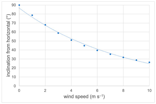
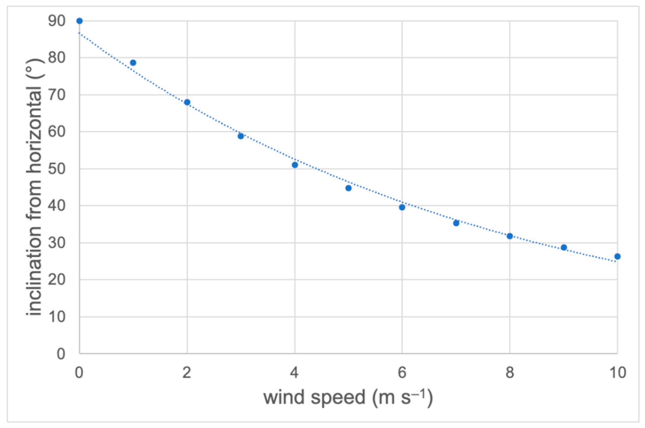
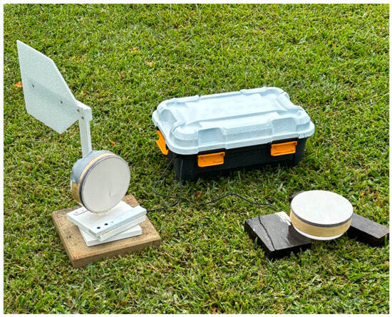
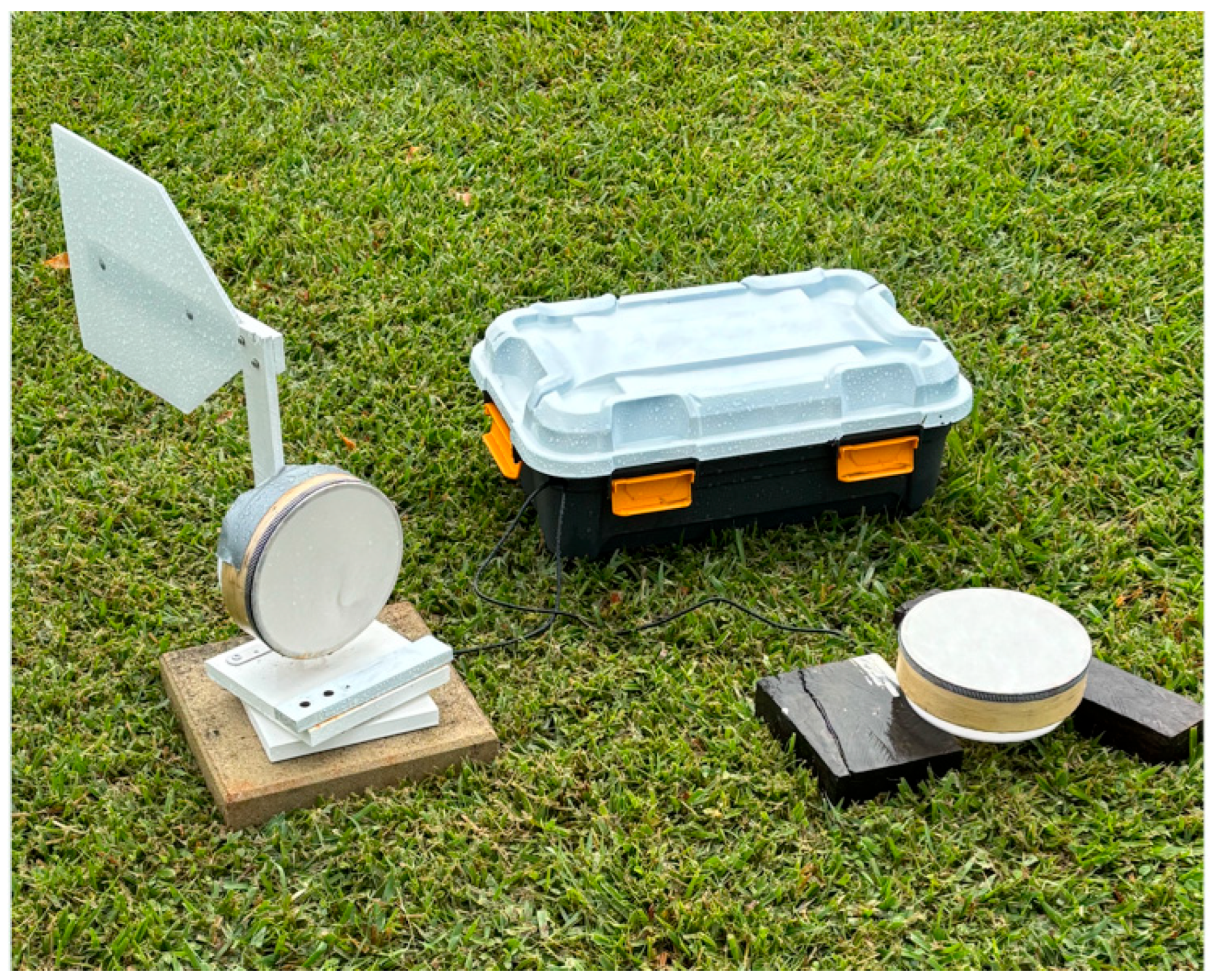
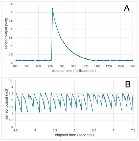
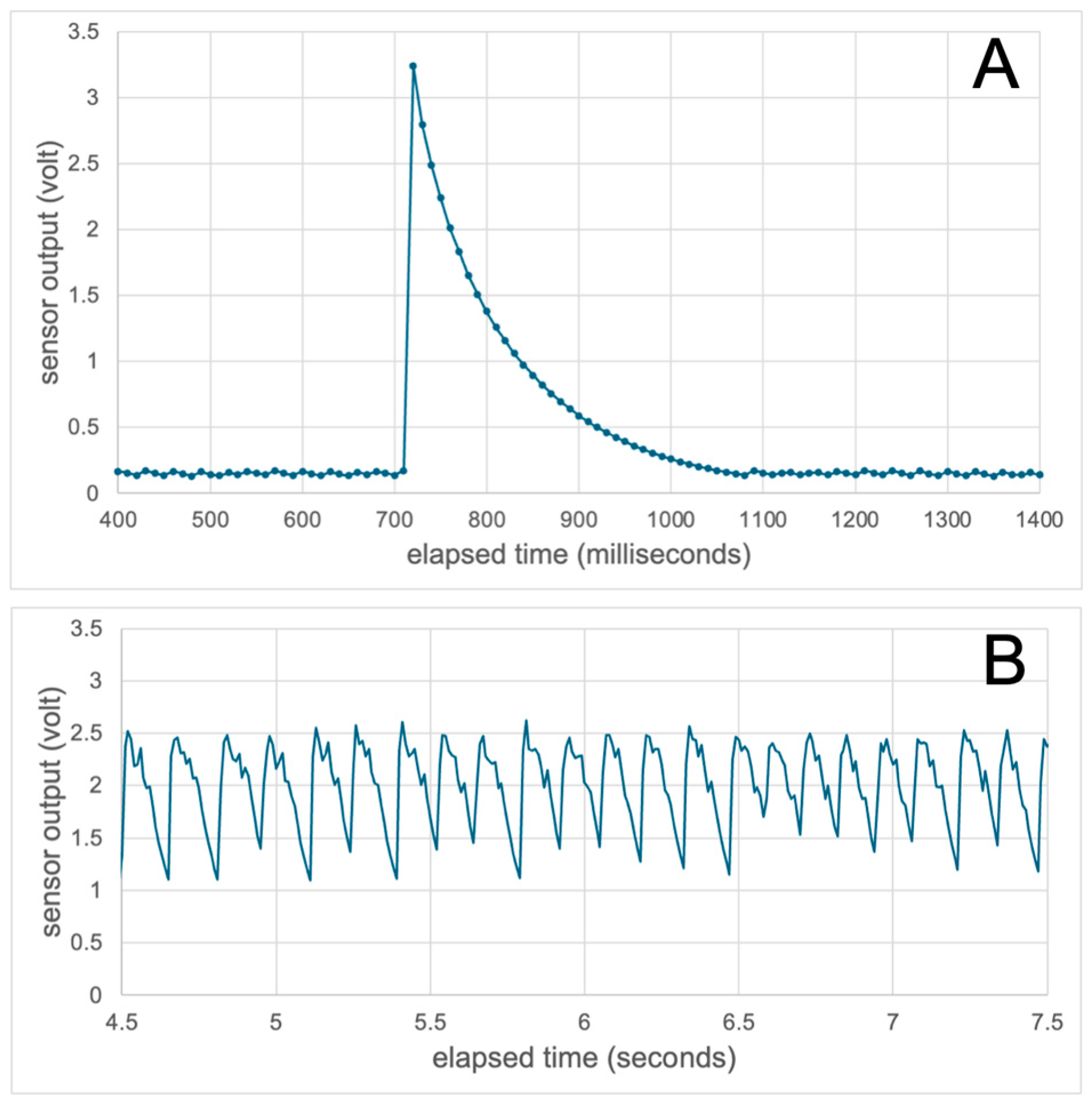
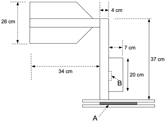
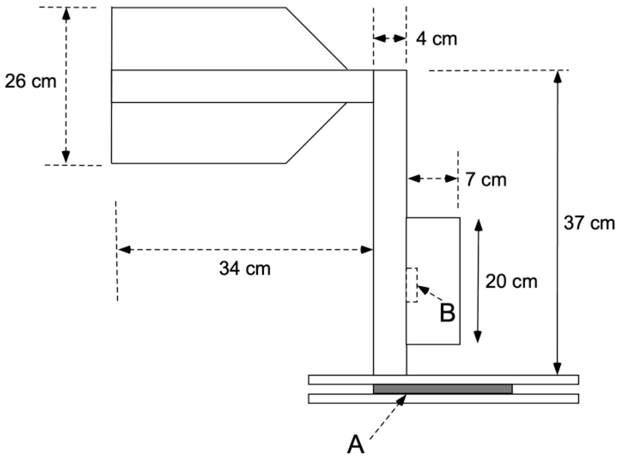
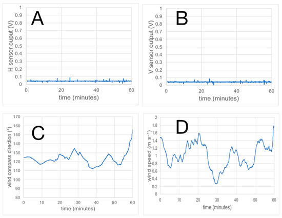
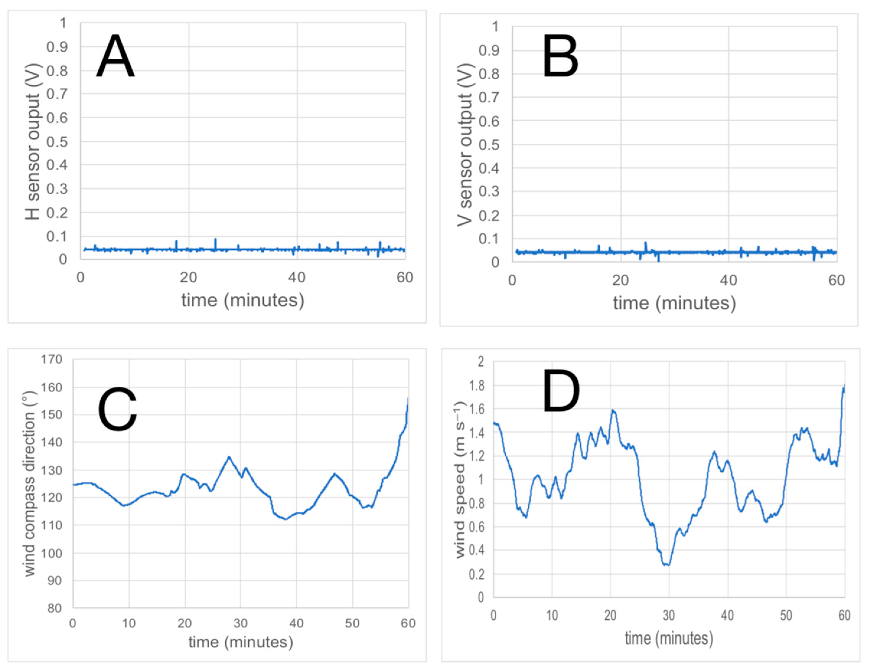
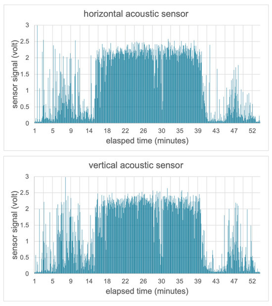
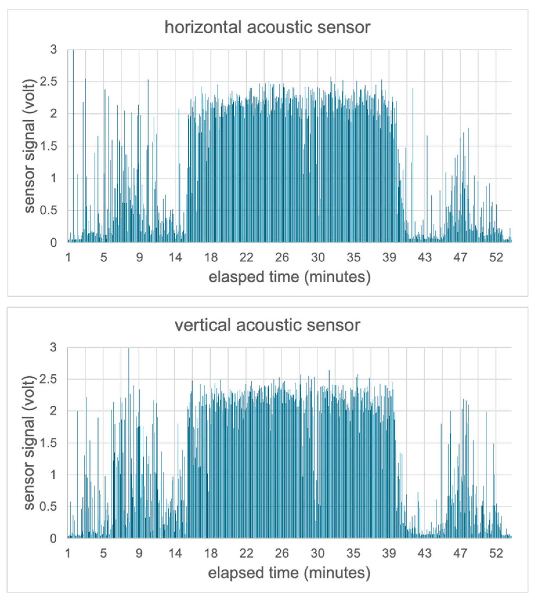
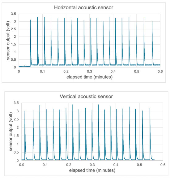
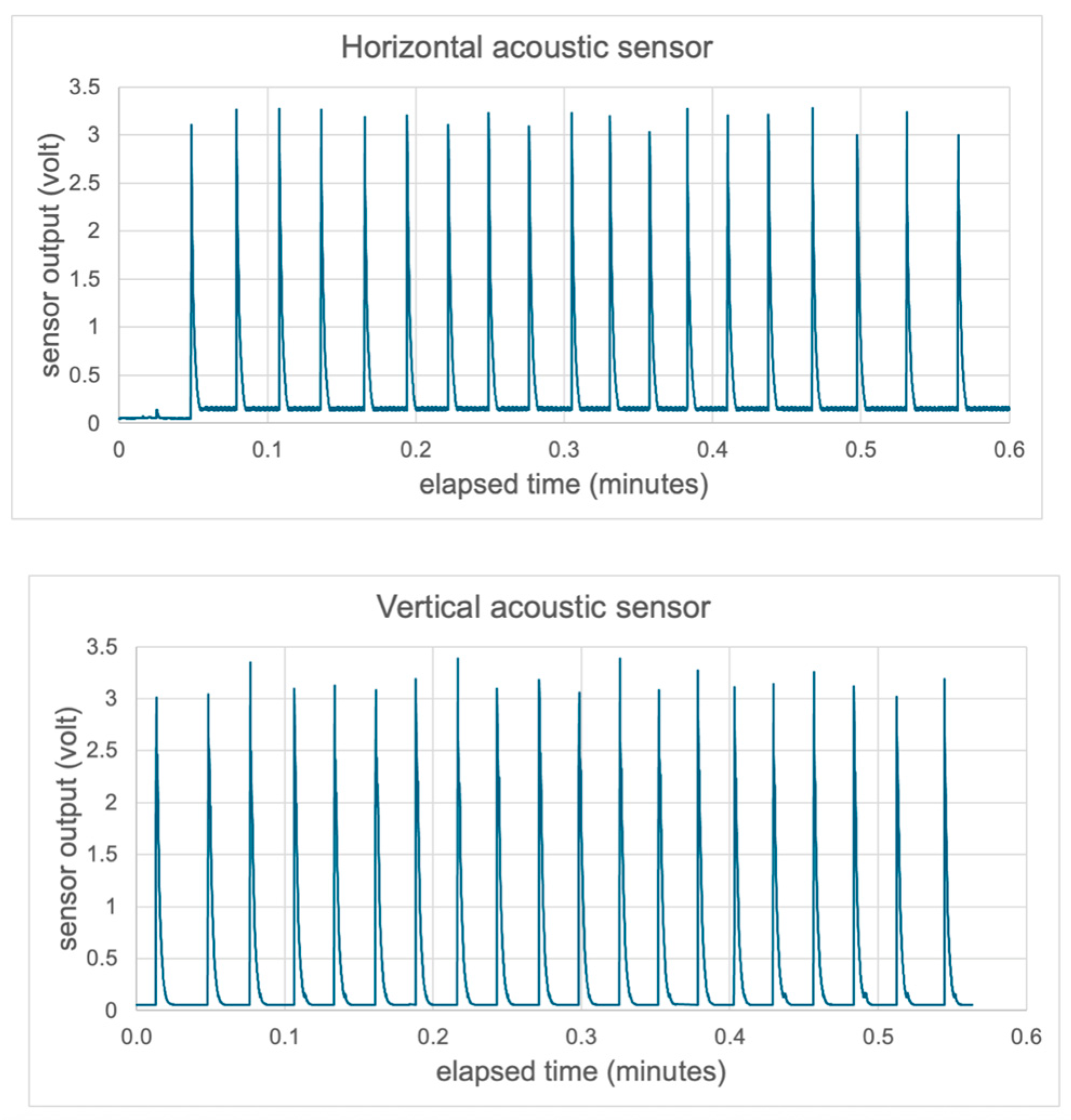
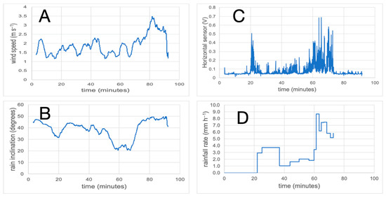
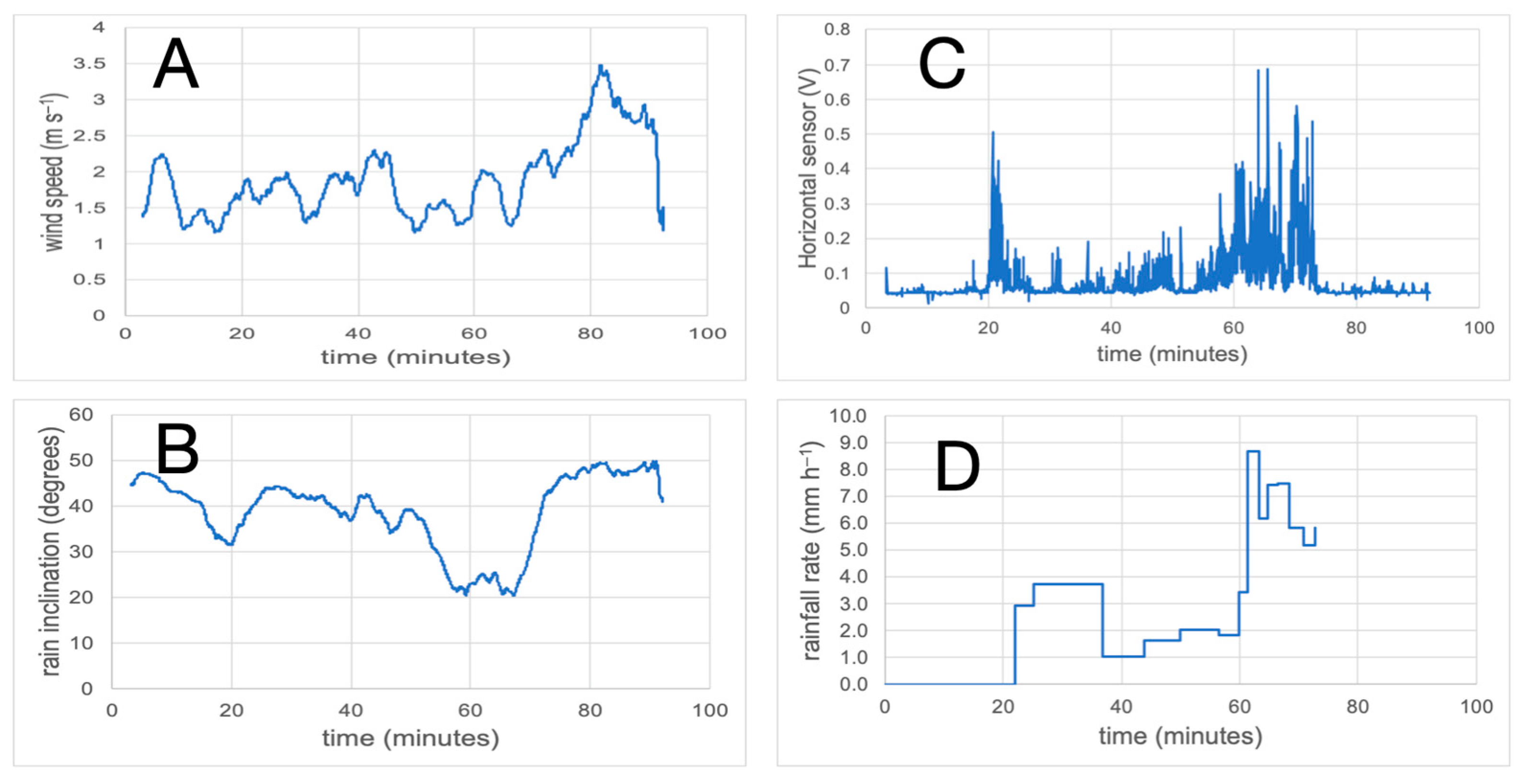
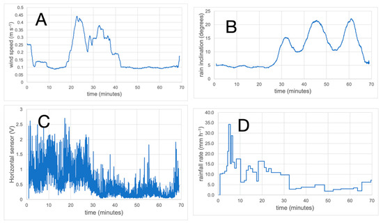
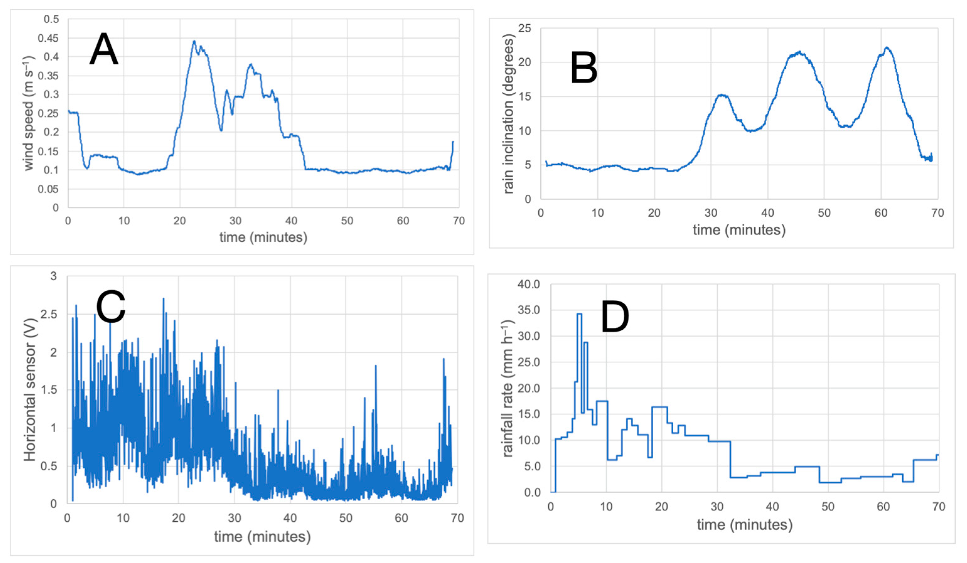

Disclaimer/Publisher’s Note: The statements, opinions and data contained in all publications are solely those of the individual author(s) and contributor(s) and not of MDPI and/or the editor(s). MDPI and/or the editor(s) disclaim responsibility for any injury to people or property resulting from any ideas, methods, instructions or products referred to in the content. |
© 2026 by the author. Licensee MDPI, Basel, Switzerland. This article is an open access article distributed under the terms and conditions of the Creative Commons Attribution (CC BY) license.