


Abstract
Meteorological drought can propagate into agricultural drought, with transition probability and timing varying across landscapes. We applied an onset-based event framework and spatial-block double machine learning (DML) with geographically weighted regression (GWR) to 48,242 eligible meteorological drought onsets across 1147 persistent cropland grids in the Yangtze River Basin during 1981–2022. Eligibility required non-drought antecedent soil moisture and a complete three-month response window. Agricultural drought occurred within this window for 35.39% of eligible events, and 56.33% of successful responses in the filtered the European Space Agency’s Climate Change Initiative root-zone soil moisture product (ESA CCI) root-zone product first crossed the drought threshold one or two months after onset (compared with 49.48% in paired ERA5-Land reanalysis). Propagation probability peaked in autumn and increased over 1981–2022. While basin-wide reservoir-distance coefficients were small with 95% confidence intervals spanning zero, local adjusted associations exhibited a consistent West–East gradient across Random Forest and LightGBM (r = 0.799; sign agreement 89.5%). The constant-coefficient restriction was rejected under conditional inference (Holm-adjusted p = 0.040), whereas conservative full-process spatial-block resampling yielded marginal support for the West–East mean contrast (p = 0.100 and 0.090). These patterns reflect covariate-adjusted spatial associations within regional hydro-environmental settings rather than causal effects of reservoir operations.
1. Introduction
The probability and timing of agricultural drought following meteorological drought vary across landscapes [1,2]. An atmospheric water deficit is transmitted through a land surface whose water storage, climate, and human use vary across space [3,4]. The Standardized Precipitation Evapotranspiration Index (SPEI) describes anomalies in the climatic water balance [5], whereas a soil-moisture index measures a different part of the drought sequence. Understanding their connection requires estimates of how often a meteorological onset is followed by soil-moisture drought, when the first response occurs, and how these quantities change across regions and periods. Specifically, we use the 1-month SPEI (SPEI-1) to pinpoint the monthly onset of an acute atmospheric water deficit at the exact temporal resolution of the monthly soil-moisture response series. While medium-term indices such as SPEI-3 or SPEI-6 integrate multi-month cumulative deficits and are widely used for seasonal drought monitoring, they blend prior climatic history into the onset timestamp and can obscure month-to-month transition lags; pairing SPEI-1 with an antecedent non-drought soil-moisture screen directly isolates short-term onset-to-response propagation timing [5].
Studies in the Yangtze River Basin have examined these connections using complementary approaches. Cross-wavelet analysis identifies phase differences among meteorological, hydrological, soil-moisture, and vegetation indices [6]. Event matching and probabilistic analysis characterize linked drought episodes [7], while multi-index comparisons examine relationships across accumulation timescales [8]. More recent work documents temporal changes in propagation risk [9]. These approaches establish substantial variability, but their probabilities and timescales depend on the index, event definition, and matching rule [10].
An onset-based event count makes the initial soil-moisture state and the response denominator explicit. Initial conditions are relevant because antecedent soil moisture can shape the development and persistence of soil-moisture drought [11,12]. If agricultural drought is already present before meteorological onset, its subsequent persistence answers a different question from the emergence of a new threshold crossing. We therefore examine meteorological onsets with non-drought soil moisture in the preceding month and record the first response within a fixed window. Separating same-month co-occurrence from lag 1–2 responses gives this event statistic a defined temporal interpretation.
Water infrastructure provides another reason for propagation relationships to vary geographically. Human water use and storage interact with drought processes [13], and studies of regulated systems show that reservoir-related changes depend on the drought variable and setting [14,15]. When basin-wide water delivery and operating records are unavailable, straight-line (haversine) distance to the nearest active large dam provides a reproducible descriptor of geographic proximity. Because straight-line distance does not measure actual hydrological connectivity via river networks or irrigation canals—nor does it record reservoir releases—it serves as a spatial proxy that also reflects dam siting and surrounding terrain; its covariate-adjusted association with drought propagation must therefore be interpreted within the regional hydrological context rather than as a direct measure of dam operations.
A single basin-wide coefficient can summarize an average association while leaving its spatial variation unresolved. Double machine learning (DML) combines flexible nuisance estimation with orthogonalized regression [16], and spatial blocking helps evaluate models with spatially structured observations [17,18]. Geographically weighted regression (GWR) allows regression coefficients to vary by location [19,20]. Combining residualization with a local second stage makes it possible to compare the constant-coefficient summary with fitted local associations, provided that surface agreement and inferential uncertainty are assessed separately.
This study addresses two linked questions across persistent cropland in the Yangtze River Basin during 1981–2022. First, what are the probability, first-response timing, seasonal differences, and long-term evolution of agricultural drought following eligible meteorological onsets? Second, how does the basin-wide adjusted reservoir-distance association compare with local relationships, and what regional environmental gradients accompany those patterns? We use monthly SPEI and root-zone soil moisture, a temporally screened large-reservoir inventory, and Random Forest (RF)- and LightGBM-based DML-GWR, followed by direct regional tests and spatial resampling checks. By combining onset-based event analysis with spatially blocked DML and GWR, this study examines both the timing of drought propagation and spatial variation in adjusted reservoir-proximity associations. The analytical approach is not restricted to the Yangtze River Basin and can be adapted to other regions with suitable drought observations and infrastructure data.
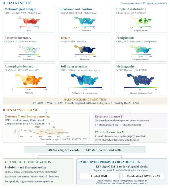
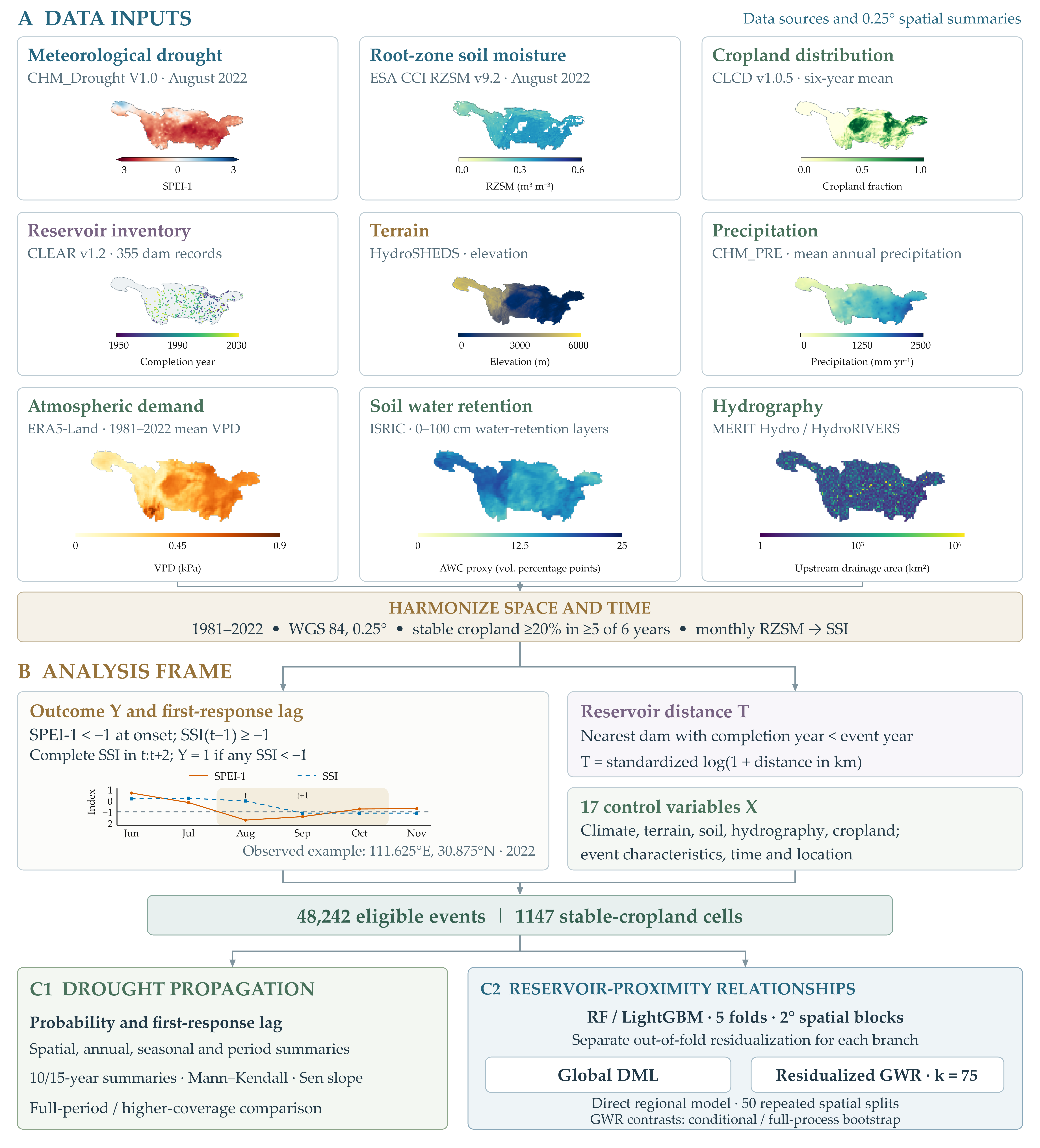
Figure 1 summarizes the event analysis, reservoir-proximity models, and regional contextual comparisons.
Figure 1.
Data sources, event construction, and analytical workflow on the 0.25° analysis grid. (A) Meteorological drought (SPEI-1), root-zone soil moisture, cropland fraction, large-reservoir inventory, terrain, precipitation, atmospheric demand, soil water retention, and hydrography, harmonized to 1981–2022 on a WGS 84 0.25° grid. (B) Event-level analysis frame: the binary outcome and first-response lag, the standardized reservoir distance, and the 17 covariates; the inset shows an observed onset at 111.625° E, 30.875° N. (C1) Event statistics and spatiotemporal summaries. (C2) Spatial-block DML, residualized GWR, the direct regional model, and spatial resampling.
2. Materials and Methods
2.1. Study Area
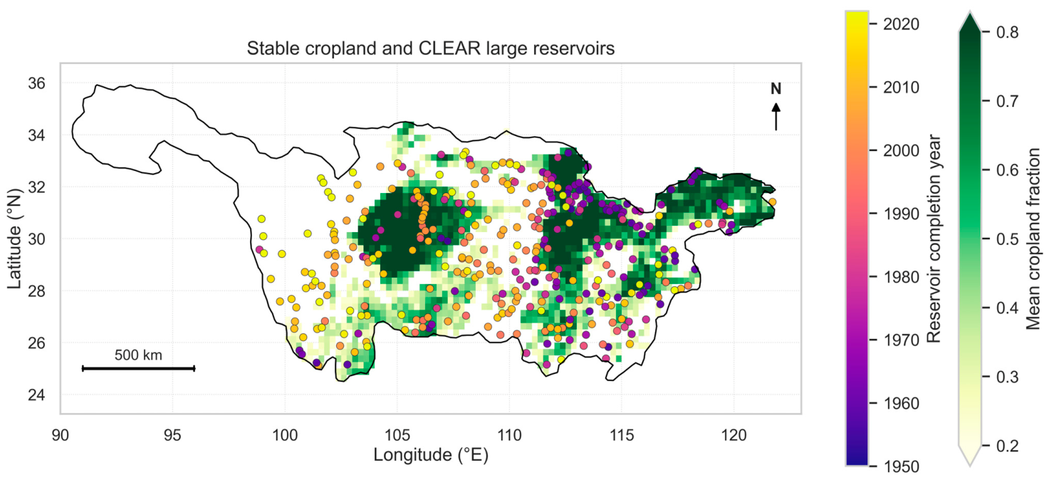
The Yangtze River Basin spans strong gradients from the Western mountain and plateau margins to the lower-elevation middle and Eastern basin (Figure 2). We describe reservoir-proximity patterns in three prespecified longitudinal sectors: western (<105° E), transition (105° E to <112° E), and eastern (≥112° E). These sectors provide a common spatial summary rather than formal hydrological subdivisions. All layers were aligned to the 0.25° WGS 84 grid of the root-zone soil-moisture product.
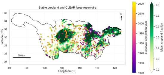
Figure 2.
Study area, persistent cropland analysis grid (0.25°), and spatial distribution of large reservoirs in the Yangtze River Basin from China Large rEservoirs Attributes and dRainage boundaries (CLEAR) v1.2 (n = 355). Sampled grids maintain at least 20% cropland coverage in at least five of six benchmark China Land Cover Dataset (CLCD) years (1985–2022). Reservoir markers show dam locations colored by completion year.
2.2. Data Sources and Preprocessing
2.2.1. Drought and Cropland Data
Meteorological drought onsets were identified using the 1-month Standardized Precipitation Evapotranspiration Index (SPEI-1) from CHM_Drought V1.0, a monthly 0.1° dataset for mainland China covering 1961–2022 [21,22]. Monthly SPEI-1 grids for January 1981–December 2022 were aggregated to the 0.25° analysis grid using area-overlapping average resampling (GDAL Resampling.average in rasterio), excluding missing values (Table S7). Months with SPEI-1 < −1.0 were defined as meteorological drought. Using SPEI-1 defines the short-term atmospheric forcing at onset, whereas the subsequent three-month soil-moisture window captures the initial root-zone threshold crossing, and the antecedent soil-moisturescreen separates newly emerging agricultural droughts from the persistence of pre-existing deficits.
Root-zone soil moisture was obtained from the daily 0.25° rzsm_1m layer of ESA CCI Soil Moisture v9.2, representing 0–1 m depth [23,24]. This product derives root-zone estimates by filtering satellite surface-soil-moisture observations; because exponential filtering smooths and can introduce phase lag into surface observations, observed root-zone first-crossing lags reflect both physical soil-water redistribution and filtering-related persistence [25]. Daily values within 0–1 m3 m−3 were averaged for months with at least five valid observations, without interpolation. Nonparametric soil-moisture standardization follows the general index approach described by AghaKouchak [26]; our implementation used Blom plotting positions. Within each grid and calendar month, observations from 1981 to 2022 were ranked with average ranks for ties, requiring at least eight valid years, and transformed to obtain the Standardized Soil-Moisture Index (SSI):
where ri,m is the rank, ni,m is the number of valid observations for the corresponding calendar month, and Φ−1 is the inverse standard normal cumulative distribution function.
Agricultural drought was defined by SSI < −1.0. The 1988–2022 period was examined separately because satellite observation coverage increased after 1987 (Figure S1; Table S2). Persistent cropland was identified from six China Land Cover Dataset (CLCD v1.0.5) benchmark maps for 1985, 1990, 2000, 2010, 2020, and 2022 [27,28]. Binary cropland masks were average-resampled from 30 m to 0.25°. Cells with valid coverage in all six maps and at least 20% cropland in five or more benchmark years formed a frame of 1279 cells; 1147 contained eligible events with complete required soil-moisture observations.
Because long-term (1981–2022), depth-matched (0–1 m) in situ soil-moisture station networks with continuous monthly coverage across the 1147 cropland grids are not publicly available at the basin scale, we evaluated the sensitivity of propagation timing to satellite exponential filtering by conducting a paired cross-product comparison against ERA5-Land monthly root-zone soil water [29]. ERA5-Land is a physically based land-surface reanalysis that simulates root-zone water balance without satellite exponential filtering. We combined the top three ERA5-Land soil layers over 0–1 m (thickness weights of 0.07, 0.21, and 0.72), aggregated them to the 0.25° grid via spherical area overlap, and applied the identical grid- and calendar-month Blom standardization over 1981–2022. Across all 43,029 common SPEI-1 onsets meeting the antecedent non-drought screen and complete [t, t + 2] window in both datasets, we compared propagation outcomes (no response, lag 0, lag 1, and lag 2) using 1999 spatial-block bootstrap resamples (Supplementary Section S17).
2.2.2. Environmental Covariates and Reservoir Data
Environmental covariates characterized climate, topography, soil, hydrography, and cropland density. Vapor pressure deficit (VPD) was derived from ERA5-Land monthly mean 2 m air temperature (T) and dew-point temperature (Td) [29]. Saturation vapor pressure was calculated as
where x denotes temperature in °C and es is expressed in kPa. Monthly VPD was then calculated as
A 0–100 cm available-water-capacity proxy was derived as the soil-layer-thickness-weighted difference between mapped water contents at 33 and 1500 kPa, expressed in volumetric percentage points [30]. Supplementary Section S9 documents the archived ISRIC layers and their processing. Monthly VPD was average-resampled to 0.25° and averaged over 1981–2022. MERIT Hydro supplied upstream drainage area and nearest-river distance [31]. HydroRIVERS supplied natural reach discharge and river-network distance to the basin outlet for contextual comparisons [32].
Elevation and finite-difference slope were derived from the 30 arc-second HydroSHEDS v1 void-filled DEM [33] and average-resampled to 0.25°. Mean annual precipitation and precipitation seasonality, defined as the coefficient of variation of the 12 calendar-month climatological means, were calculated from CHM_PRE V2.1 for 1981–2022 [34]. The six-benchmark-year mean cropland fraction completed the biophysical controls (Table 1).
Table 1.
Data sources and their roles in the analysis.
Dam locations, completion years (COMY), and total storage capacities (TSC, km3) came from China Large rEservoirs Attributes and dRainage boundaries (CLEAR v1.2) [35]. The audited Yangtze subset contains 355 large reservoirs with complete storage capacities. Of these, 210 were completed within 1981–2022 and 122 before 1981; the remaining 23 have completion years after 2022 and never enter the treated set. Observed dam coordinates were used where available, with MERIT-aligned coordinates as fallback. A reservoir was active for an event only when COMY was strictly less than the event year; because the last event year is 2022, the eight reservoirs completed in 2022 never enter the active set.
2.3. Event-Based Drought Propagation Analysis
2.3.1. Identification of Meteorological-to-Agricultural Drought Propagation
Consecutive months with SPEI-1 < −1.0 within a grid cell were grouped into a single meteorological drought spell, with onset month t defined as the first month of the spell. Collapsing multi-month spells to their initial onset ensures that each drought episode contributes a single onset observation.
Eligibility required SSIi,t−1 ≥ −1 and valid SSI in each month from t through t + 2. This excludes events with pre-existing agricultural drought or incomplete response windows; missing SSI was never coded as absence of propagation. For event e in grid i, the binary outcome was defined as
where Yi,e = 1 indicates that agricultural drought occurred within [t, t + 2] for event e in grid cell i. For propagated transitions (Yi,e = 1), the first-response lag was defined as
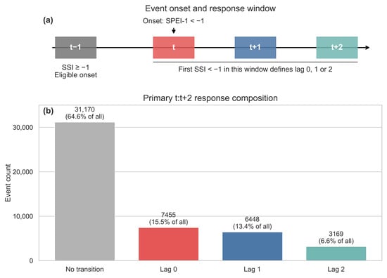
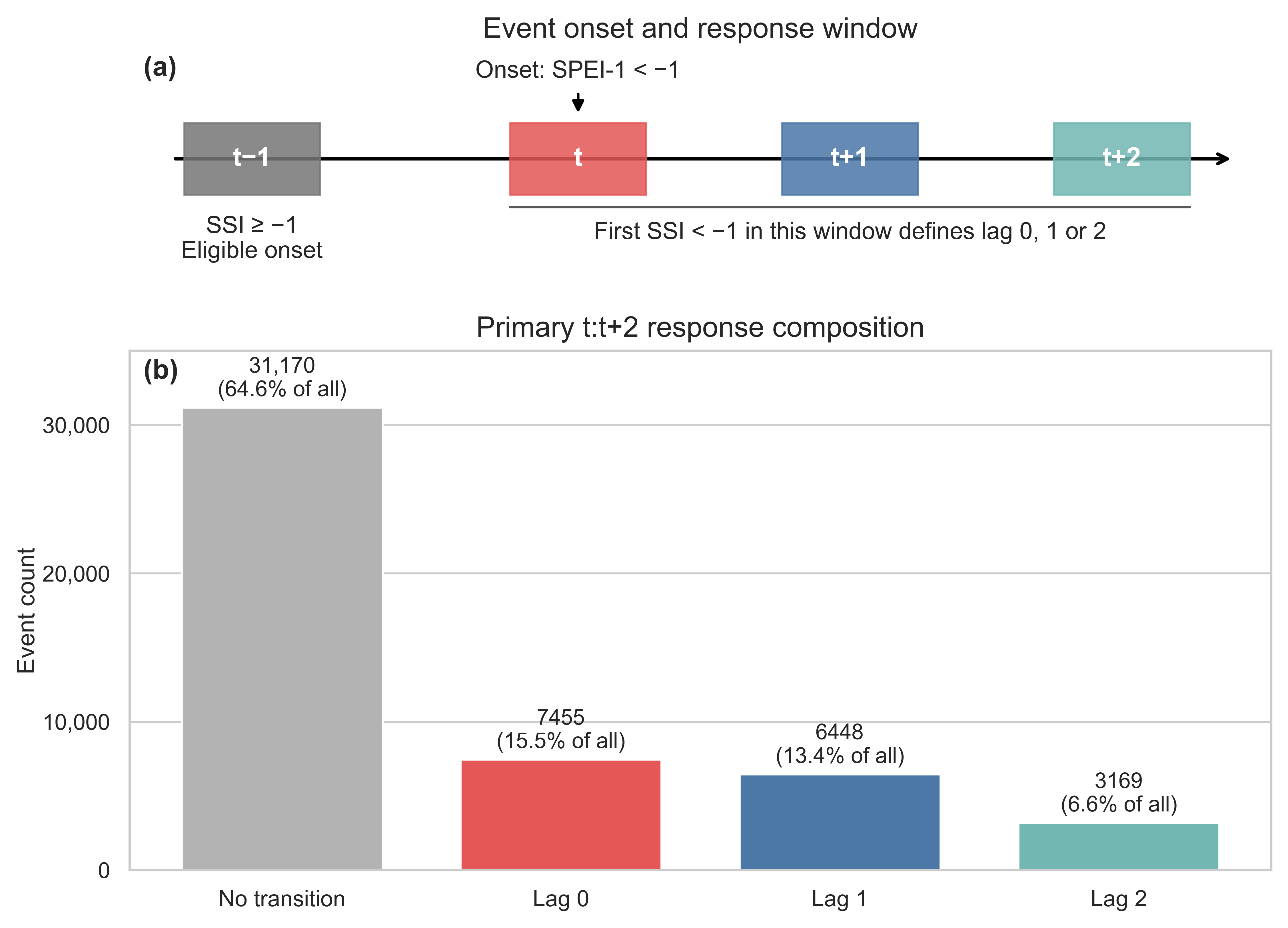
Here, L = 0 denotes same-month SSI threshold crossing or co-occurrence; monthly observations do not establish the order of the two drought onsets within that month. Values of L = 1 or 2 identify first responses in the following one or two months (Figure 3).
Figure 3.
Event eligibility and first-response composition. (a) SSI(t − 1) ≥ −1 and SPEI-1(t) < −1 define an eligible meteorological onset, subject to complete SSI observations in [t, t + 2]. The first SSI < −1 identifies lag 0, 1, or 2. Lag 0 denotes same-month co-occurrence. (b) Counts and percentages among 48,242 eligible events. Of 17,072 successful responses, 43.67% occurred at lag 0 and 56.33% at lag 1–2.
Alternative windows were evaluated using their corresponding complete-observation requirements: [t], [t, t + 1], [t, t + 2], [t + 1, t + 2], and [t + 1, t + 3] (Table S1). An event-level audit reproduced the primary outcome and first-response lag for all 48,242 events and confirmed the antecedent criterion. The latest eligible onset was October 2022; later onsets lacking a complete window were excluded (Supplementary Section S15).
2.3.2. Spatiotemporal Analysis of Drought Propagation
Grid-level propagation probability was calculated as the ratio of propagated transitions to eligible events, accompanied by the mean and median first-response lag. Basin-scale probabilities pooled eligible events by calendar year, onset season (December–February [DJF], March–May [MAM], June–August [JJA], and September–November [SON]), and decadal periods, with 10- and 15-year moving windows summarizing decadal variability.
Trends in annual event-pooled propagation probability were summarized using the Mann–Kendall test [36], Sen slope [37], and Hamed–Rao variance adjustment [38]. Sen confidence intervals were not serial-correlation-adjusted. The Hamed–Rao implementation screened all available lags; only lag 14, with negative autocorrelation, contributed to its adjustment (Table S8; Supplementary Section S10). Coverage-period sensitivity compared the 1981–2022 and 1988–2022 probability maps across all 1147 common grids. Top-quintile hotspot overlap used 1145 grids with at least ten eligible events in both periods. An alternative SSI reference period is examined in Supplementary Section S15.
2.4. Reservoir-Proximity Modeling via Spatial-Block DML and DML-GWR
2.4.1. Dynamic Reservoir-Proximity Representation
For each cropland grid and event year, reservoir proximity was the haversine distance from the grid center to the nearest active large-reservoir dam (Earth radius, 6371.0088 km). We standardized log(1 + distance in km) using the mean (3.738755) and standard deviation (0.739312) of the balanced 1279-grid, 42-year panel. This fixed scaling makes coefficients comparable across the analyses. A positive distance coefficient corresponds to higher adjusted propagation probability farther from a dam; a negative coefficient corresponds to higher probability closer to a dam. Filtering by completion year (COMY < event year) ensures temporal consistency in the historical infrastructure inventory, while the resulting distance metric characterizes adjusted geographic proximity rather than verified canal or river water delivery to a specific grid cell.
2.4.2. Basin-Wide Spatial-Block Double Machine Learning
The basin-wide adjusted relationship was estimated using the partially linear DML model [16]. In the regression equations below, i indexes eligible event observations (N = 48,242); grid membership determines spatial blocks and local weights:
where Yi is the binary propagation outcome, Ti is standardized log-distance, θ is the constant basin-wide coefficient, and g(Xi) describes the relationship with the covariate vector Xi. The 17 controls were mean annual precipitation, precipitation seasonality, climatological VPD, elevation, slope, log upstream drainage area, nearest-river distance, soil available-water-capacity proxy, mean cropland fraction, event minimum SPEI-1, spell duration, onset-month sine and cosine, centered year and its square, longitude, and latitude.
Minimum SPEI and duration describe the full meteorological drought spell, including information after onset. The 17-control analysis is therefore a retrospective adjusted-association analysis. A sensitivity analysis removed these two variables, retained the same events and spatial folds, and refitted both nuisance functions (Supplementary Section S11).
The two first-stage nuisance functions are
Both conditional expectations were estimated separately using RF [39] and LightGBM [40] regressors; complete settings are given in Table S6 (Supplementary Section S8).
Cross-fitting kept every event within a 2° × 2° spatial block in the same fold, following the use of blocked validation for spatially structured data [17,18]. The 44 occupied blocks were assigned to five folds, stratified by active-reservoir presence within 100 km. Each event received nuisance predictions from models trained on the other four folds. The global and local models used their respective fold partitions, and the direct regional comparisons were performed using the same fold partition as the local model. To verify first-stage nuisance-model quality, we evaluated out-of-fold (OOF) prediction performance across all 48,242 events using root mean squared error (RMSE) and R2 for both the outcome and treatment regressions, alongside the standard deviation of the residualized treatment (Supplementary Table S26). Out-of-fold residuals were
where k(i) denotes the spatial fold containing observation i and (−k(i)) indicates out-of-fold prediction from models trained on the remaining four folds. Throughout Equations (10)–(12), and denote these orthogonalized residuals; the unadjusted variables appear only in Equation (7).
The basin-wide DML coefficient was then obtained via no-intercept residual-on-residual regression:
Because T uses fixed-panel scaling, multiplying by 100 expresses the association in propagation-probability percentage points per one-SD increase in log-distance. Primary global intervals used influence-function standard errors clustered by the 44 spatial blocks with a normal approximation. The accompanying 499-draw block bootstrap held the first-stage residuals fixed and is a conditional interval.
2.4.3. Second-Stage DML-GWR for Spatially Varying Relationships
The local analysis combined out-of-fold residualization with geographically weighted regression. DML motivates orthogonalization against observed covariates [16], while residual-based heterogeneous-effect learning and GWR provide related approaches to variation in regression relationships [19,20,41]. Here, the combined procedure estimates spatially varying adjusted associations.
At each target grid center s, the second-stage local linear model was specified as
where and are the out-of-fold orthogonalized outcome and treatment residuals, α(s) is a local intercept capturing neighborhood-level residual baseline differences, and θ(s) is the local reservoir-distance slope at location s.
Local parameters were estimated by geographically weighted least squares using grid-level sufficient statistics:
where wi(s) is the spatial kernel weight assigned to observation i when estimating the coefficient at target grid s.
Spatial weights followed an adaptive bisquare kernel:
where di(s) is the haversine distance between observation i and target grid s, and bs is the adaptive distance bandwidth. In the full-sample surface, the k-nearest candidate grids (including the target grid) receive positive bisquare weights and the (k + 1)-th ordered distance defines the zero-weight boundary, whereas in leave-block-out cross-validation, the boundary is set at the k-th retained out-of-block distance with a negligible numerical tolerance.
Bandwidth was selected by leave-spatial-block-out cross-validation mean squared error (CV MSE) over the candidate grid counts from 50 to 1147. For each target grid, all grids in its 2° block were excluded from the local validation fit. Both primary searches selected k = 75 (Table S3). This second-stage bandwidth validation used the first-stage residuals; outer-block prediction evaluations are summarized in Supplementary Section S14. To verify that selecting k = 75 does not over-smooth spatial heterogeneity across the 1147 grids, we conducted a bandwidth sensitivity analysis comparing fitted local surfaces, regional means, sign concordance, and effective neighborhood support across k = 50, 75, and 100 while holding first-stage OOF residuals and fold partitions fixed (Supplementary Section S16).
Local slopes are expressed in the same percentage-point-per-SD units as the global coefficient. The maps display the fitted point estimates without a significance mask.
Surface agreement was assessed using Pearson and Spearman correlations and sign concordance. Equal-grid local means and sign proportions were summarized for the Western (longitude < 105° E), transition (105° E ≤ longitude < 112° E), and Eastern (longitude ≥ 112° E) sectors.
2.5. Regional Inference, Stability, and Hydrological Context
A direct three-region model regressed the out-of-fold outcome residual on the treatment residual interacted with the three prespecified region indicators, without a separate intercept. It estimated West, transition, and East coefficients and the contrast Δ = θWest − θEast. We used CR1 standard errors clustered by the 44 spatial blocks and t-based intervals, supplemented by 1999 fixed-residual block-bootstrap draws and leave-one-block-out diagnostics. West, transition, and East contained 10, 19, and 19 blocks, respectively; some blocks crossed sector boundaries. Sensitivity to the 29 blocks represented in the West–East contrast is reported alongside the primary 43-degree-of-freedom calculation (Supplementary Section S11).
For the GWR surface, the conditional heterogeneity analysis used 499 block-level Rademacher multiplier draws under a constant residual-slope null, holding nuisance residuals and k = 75 fixed. Holm correction [42] covered four tests: spatial heterogeneity and the West–East mean-slope contrast for each learner. A separate 199-draw full-process block bootstrap refitted both nuisance models, regenerated residuals, and reselected bandwidth. We report its centered tests and percentile intervals, alongside fixed-k sensitivity, without treating it as equivalent to the conditional multiplier test (Supplementary Section S12).
Implementation stability was examined across 50 repeated five-fold spatial partitions, with both bandwidth reselection and fixed-k versions. Other analyses used equal-grid weighting, the 1988–2022 period, and a strictly lagged [t + 1, t + 3] window. Surface agreement and Moran’s I of the grid-mean first-stage residuals were computed using eight-nearest-neighbor weights and 499 permutations. As detailed in Supplementary Section S14, outer-block records provide a separate paired comparison of global and local prediction errors on the same held-out observations.
To place the coefficient surfaces in their hydrological context, each grid was assigned to a fixed distance group using its mean active-dam distance across eligible event years: <25 km, 25–50 km, or >50 km. We compared equal-grid means of propagation probability, elevation, slope, cropland fraction, and natural river discharge within sectors. These groups summarize dynamically calculated distances but are not reassigned for each event. Prespecified near-minus-far probability contrasts used 1999 spatial-block bootstrap draws. Supplementary Section S13 reports grid, event, and block support and the sensitivity of group interpretation to changing reservoir activity.
2.6. Use of Artificial Intelligence Tools
During the preparation of this manuscript, the authors used ChatGPT (GPT-6 Astra, OpenAI) exclusively for language editing and to check and refine the Python 3.10.21 scripts for data processing, statistical analysis, and visualization. All data processing, statistical modeling, calculations, and figure generation were independently conducted and executed by the authors using Python. The AI tool was not used to generate, alter, or fabricate any research data, statistical results, figures, or scientific conclusions. The authors have reviewed and edited the output and take full responsibility for the content of this publication.
3. Results
3.1. Frequency and Lag of Drought Propagation
Across 1147 persistent cropland grids, 48,242 meteorological drought onsets met the antecedent soil-moisture and complete-response-window requirements during 1981–2022. Agricultural drought occurred within the onset month and the following two months for 17,072 events (35.39%); the remaining 31,170 events did not cross the SSI threshold during that window (Table 2).
Table 2.
Eligible meteorological drought onsets, propagation outcomes, and first-response lag distribution (1981–2022).
Delayed responses accounted for 56.33% of the 17,072 successful propagation events. The first SSI threshold crossing occurred in the onset month for 7455 events (43.67%), one month later for 6448 (37.77%), and two months later for 3169 (18.56%). The mean first-response lag was 0.75 months and the median was one month (Figure 3b). These counts distinguish same-month co-occurrence from the 9617 responses first observed at lag 1 or 2.
In the paired cross-product sensitivity analysis across the 43,029 common eligible onsets (1147 grids; 44 spatial blocks), overall propagation probability was 33.74% for ESA CCI and 47.05% for ERA5-Land. Crucially, delayed first responses (lag 1–2) accounted for nearly half or more of successful propagation events in both datasets: 58.09% in ESA CCI and 49.48% in ERA5-Land (paired ERA5-Land minus ESA CCI difference of −8.61 percentage points; 95% block-bootstrap CI, −11.56 to −5.57). When evaluated across all 43,029 common eligible onsets, lag 1–2 transitions occurred in 19.60% of events for ESA CCI and 23.28% for ERA5-Land (Supplementary Tables S24 and S25; Figure S4). These results indicate that the 1–2 month propagation lag is not solely an artifact of satellite exponential filtering, since a substantial delayed share is also present in an independent reanalysis; the exact lag proportions vary with the soil-moisture representation and the response denominator.
3.2. Spatial Pattern and Long-Term Evolution of Drought Propagation
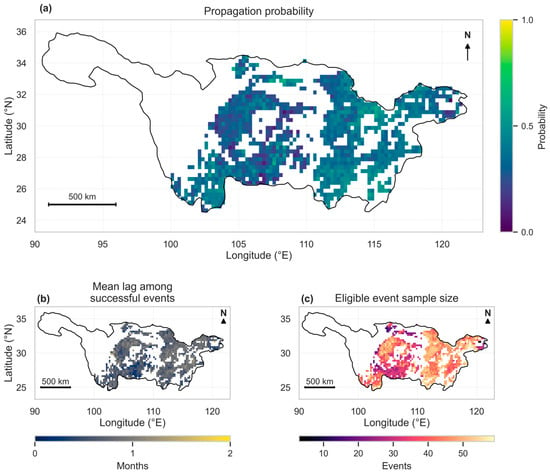
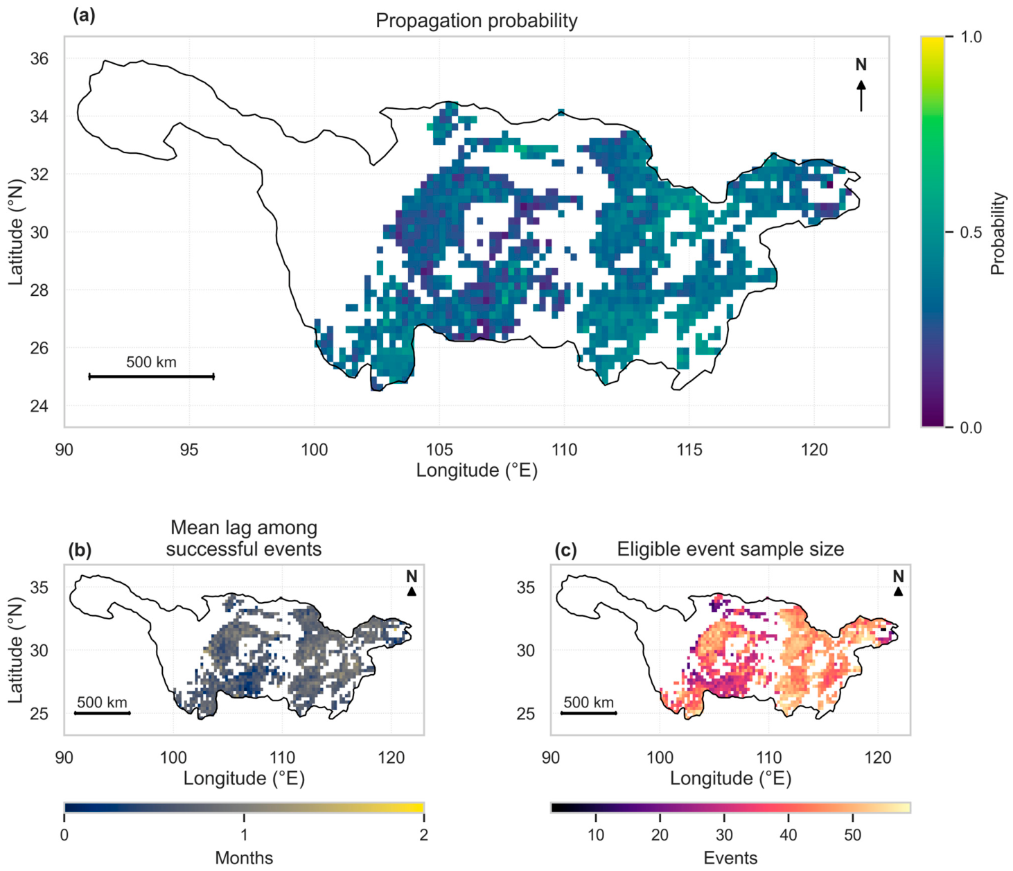
Propagation probability and first-response lag varied across the cropland network (Figure 4). Higher probabilities were concentrated in parts of the middle and lower basin, while many Western grids had more moderate probabilities. Event counts also varied: the median was 44 eligible onsets per grid, with an interquartile range of 36–49 and a range of 3–59. Event counts provide the sampling context for interpreting the probability map.
Figure 4.
Spatial characteristics of meteorological-to-agricultural drought propagation across 1147 persistent cropland grids during 1981–2022: (a) propagation probability; (b) mean first-response lag among propagated events; and (c) eligible event count per grid.
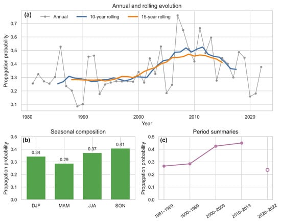
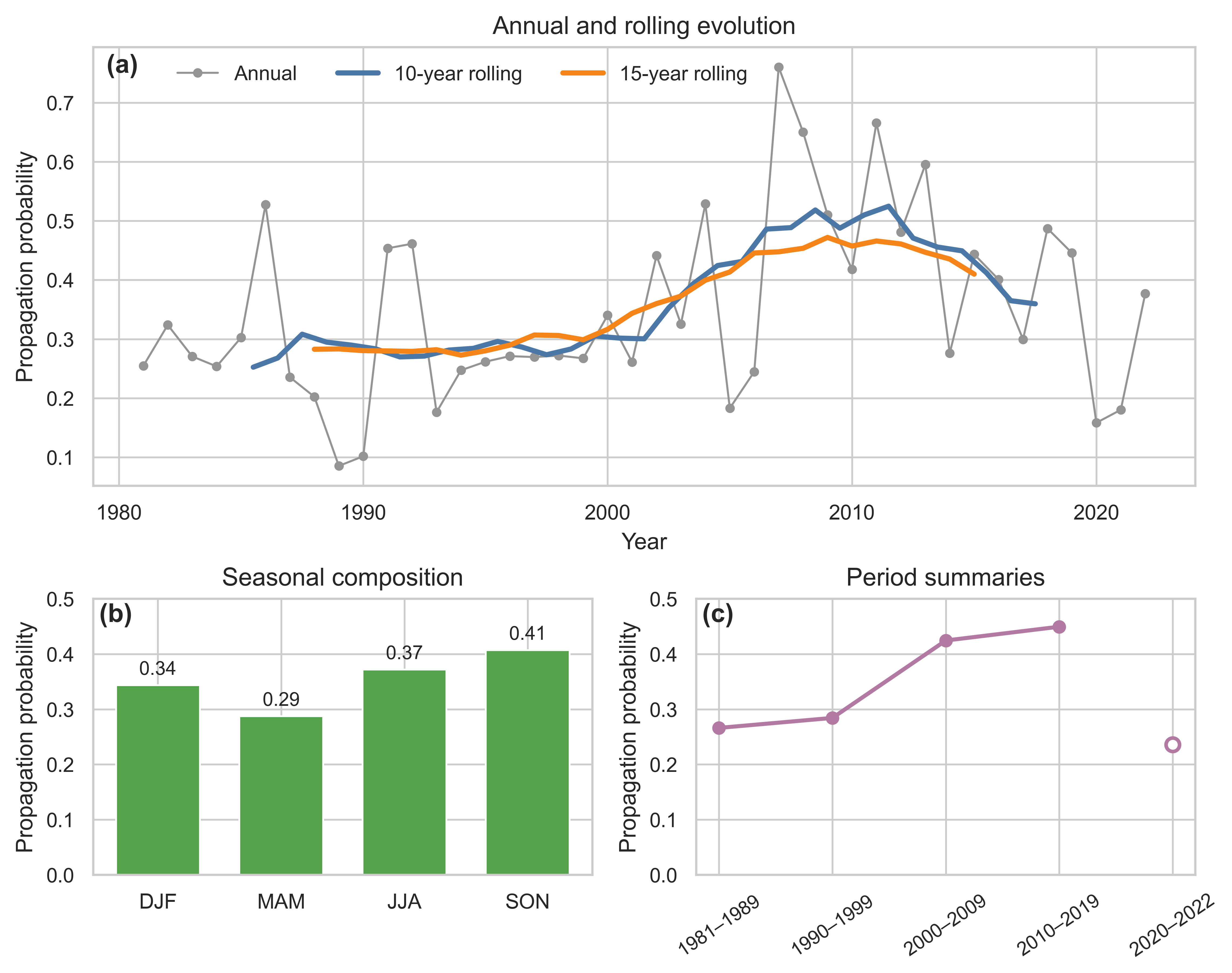
Annual event-pooled propagation probability increased in the primary specification (Figure 5a). The Sen slope was +0.39 percentage points per year over 1981–2022 (95% CI, +0.01 to +0.80; Mann–Kendall p = 0.0416) and +0.69 over 1988–2022 (+0.03 to +1.08; p = 0.0356). The corresponding Hamed–Rao tests gave p = 0.0248 and 0.0237 (Table S8). An alternative SSI reference period retained positive slopes but weakened the full-period test (Mann–Kendall p = 0.114; Hamed–Rao p = 0.081; Supplementary Section S15). The two primary-period probability maps were closely aligned across 1147 common grids (r = 0.966); hotspot overlap was 0.691 among the 1145 grids with at least ten events in both periods.
Figure 5.
Temporal evolution and seasonal composition of propagation probability (1981–2022). (a) Annual event-pooled probability and 10- and 15-year moving averages. (b) Propagation probability by meteorological onset season (DJF, MAM, JJA, SON). (c) Pooled probabilities by period (with the partial 2020–2022 window shown as an open marker).
Autumn onsets had the highest propagation probability (40.73%), followed by summer (37.18%), winter (34.38%), and spring (28.75%; Figure 5b). Period-pooled probabilities increased from 26.62% in 1981–1989 and 28.42% in 1990–1999 to 42.44% in 2000–2009 and 44.93% in 2010–2019. The final three-year interval, 2020–2022, had a lower probability of 23.59% (Figure 5c), showing that the long-term increase was not a monotonic sequence of period means.
3.3. Basin-Wide Association and Local Bandwidth
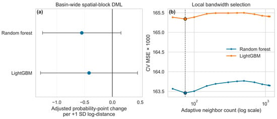
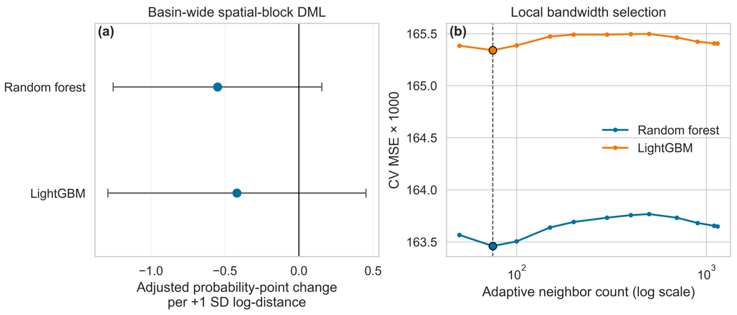
The global DML estimates indicated a weak, statistically nonsignificant average reservoir-distance association across the basin under both learners (Table 3; Figure 6a). A one-standard-deviation increase in log-distance was associated with a −0.55 percentage-point change in propagation probability under RF (95% CI, −1.25 to +0.15; p = 0.1259) and −0.42 under LightGBM (−1.29 to +0.45; p = 0.3459). Because both 95% confidence intervals spanned zero, the basin-wide average model provides no evidence of a uniform drought-mitigation effect of reservoir proximity across Yangtze cropland. Re-estimating the same specification for 1988–2022 and for a strictly lagged [t + 1, t + 3] response window left both coefficients negative, with intervals that still included zero (Table S5; Supplementary Section S7). These constant-coefficient estimates summarize the basin-wide relationship and motivate the local GWR analysis below to examine whether opposing regional relationships are masked by the basin-wide average.
Table 3.
Global adjusted reservoir-distance associations. Estimates and 95% normal block-clustered confidence intervals are in probability percentage points per one-SD increase in log-distance.
Figure 6.
Basin-wide DML estimates and GWR bandwidth selection. (a) Global spatial-block DML point estimates and 95% block-clustered confidence intervals (percentage-point change per +1 SD log-distance). (b) Leave-spatial-block-out GWR cross-validation error (CV MSE × 1000) across candidate neighbor counts k, showing a shared minimum at k = 75 for both learners.
The primary bandwidth searches selected k = 75 neighboring grids for both residualization learners, with an interior minimum in leave-spatial-block-out CV MSE (Figure 6b; Table S3). This bandwidth was retained for the principal local coefficient maps and their descriptive regional summaries. Sensitivity checks at k = 50 and k = 100 confirmed high spatial stability relative to the primary k = 75 surface: Pearson correlations ranged from 0.960 to 0.983 and grid-level sign agreement ranged from 92.4% to 96.1% across both learners. In all six learner-by-bandwidth fits, the Western regional mean remained consistently positive (+1.15 to +2.05 percentage points per SD) and the Eastern regional mean remained consistently negative (−0.88 to −1.04 percentage points per SD), yielding stable West–East contrasts of +2.13 to +2.69 percentage points per SD under RF and +2.93 to +3.02 under LightGBM (Supplementary Tables S22 and S23; Figure S3). Thus, the large-scale West–East spatial pattern is robust across neighborhood sizes and is not an artifact of over-smoothing at k = 75.
3.4. Spatially Contrasting Reservoir-Proximity Associations
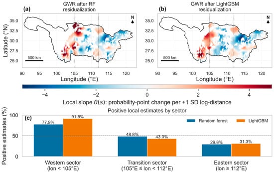
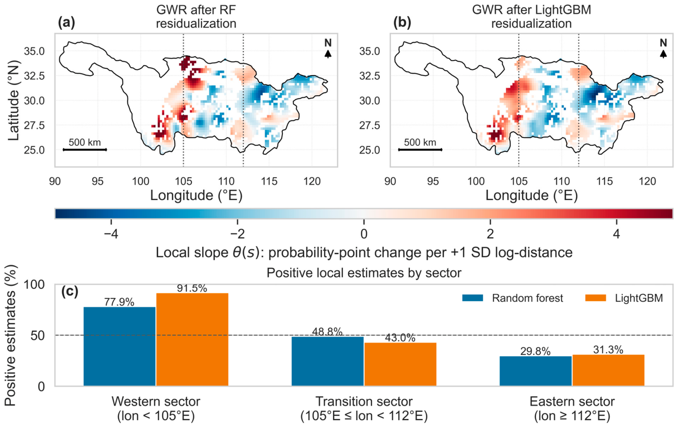
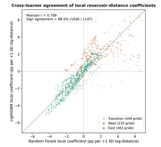
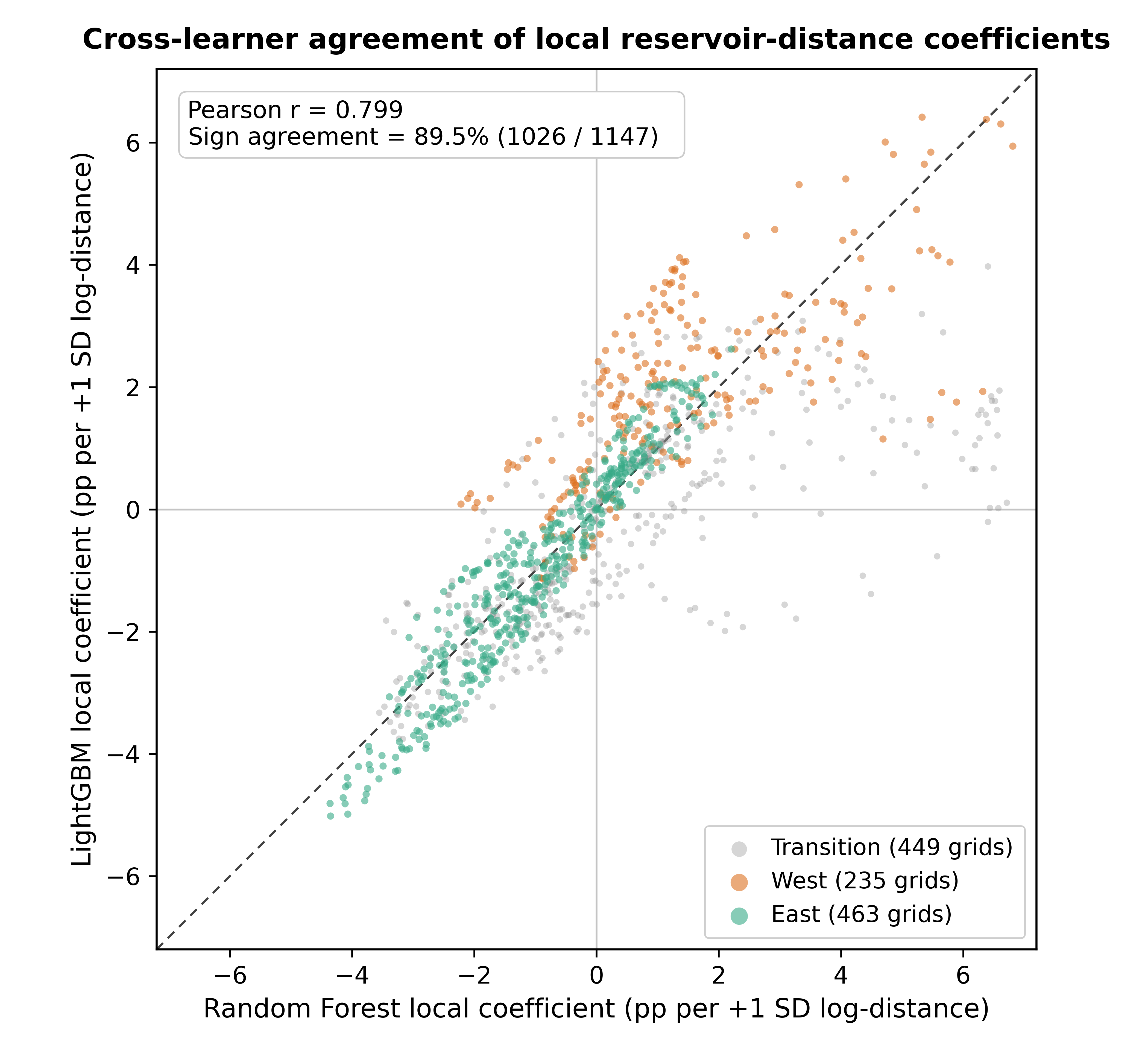
The fitted local coefficient surfaces showed a consistent broad spatial contrast across the two learners (Figure 7). Their Pearson correlation was 0.799, their Spearman correlation was 0.869, and their signs agreed at 89.5% of the 1147 mapped grids. Equal-grid mean slopes across the whole basin were +0.04 percentage points per SD under RF and −0.14 under LightGBM.
Figure 7.
Fitted local reservoir-proximity associations at k = 75. (a,b) Local coefficients after RF and LightGBM residualization, in propagation-probability percentage points per one-SD increase in log-distance. Red indicates a positive distance association and blue a negative association. Dotted lines mark 105°E and 112°E. (c) Proportion of positive point estimates by sector. Maps show all 1147 estimates and do not display a significance mask. Mapped colors and sector sign proportions represent local point estimates rather than cell-level statistical significance; because adaptive neighborhoods overlap across adjacent grids, regional uncertainty is evaluated separately via spatial-block resampling in Section 3.5.
Positive local coefficients predominated in the Western sector (<105° E): 183 of 235 grids under RF (77.9%) and 215 under LightGBM (91.5%), with regional means of +1.43 and +2.01 percentage points per SD. Negative coefficients predominated in the Eastern sector (≥112° E): 325 of 463 grids under RF (70.2%) and 318 under LightGBM (68.7%), with means of −0.98 and −1.00. The 449 transition-sector grids had mixed signs (Table 4). The resulting West-minus-East differences between equal-grid local means were +2.42 and +3.02 percentage points per SD (Table 5).
Table 4.
Signs of fitted local reservoir-distance coefficients by longitudinal sector. These are descriptive counts of the 1147 mapped point estimates, not counts of statistically significant coefficients.
Table 5.
Agreement and stability of reservoir-proximity associations. Coefficients and contrasts are in percentage points per one-SD increase in log-distance. Conditional tests retain the first-stage residuals; full-process resampling refits them. West–East contrasts are computed from unrounded equal-grid means. Direct regional-model contrasts are reported in the text and in Supplementary Table S9.
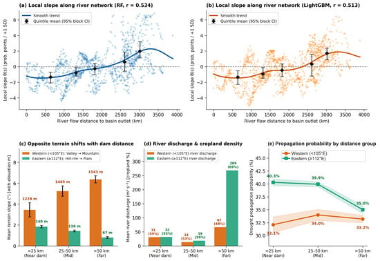
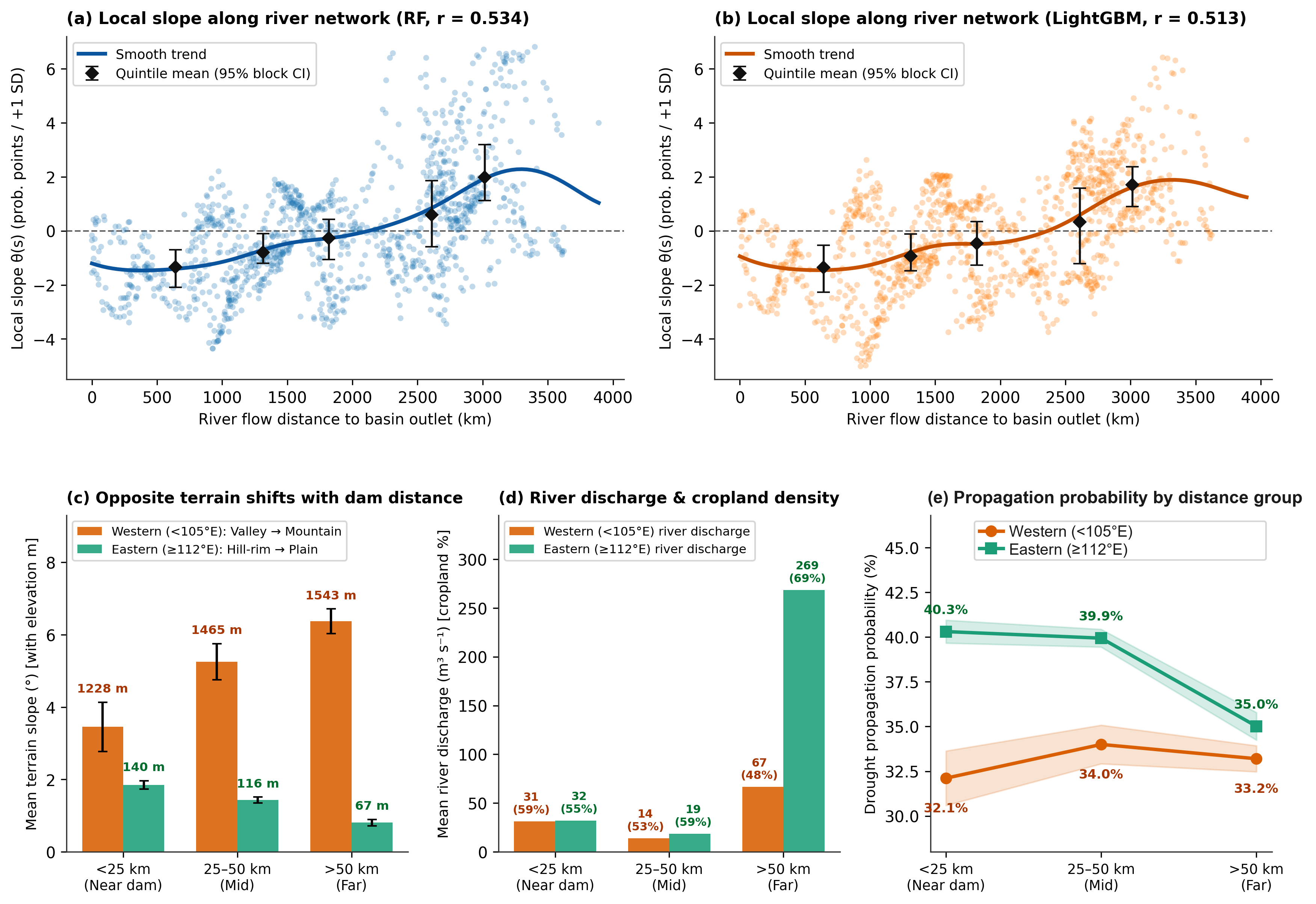
The environmental profiles varied with reservoir distance in different ways across the two sectors (Table 6; Figure 8). In the West, near-dam grids (<25 km) had lower mean elevation and slope than far-dam grids (>50 km): 1228.2 versus 1543.4 m and 3.46° versus 6.37°. Their mean cropland fractions were 59.5% and 47.7%. Propagation probabilities were 32.11%, 34.00%, and 33.20% across the near, intermediate, and far groups, respectively. The near-minus-far contrast was −1.09 percentage points (95% spatial-block bootstrap CI, −4.84 to +3.53); the near group contained only 19 grids in seven blocks.
Table 6.
Environmental profiles and propagation probability by sector and reservoir-distance group. Each grid is classified by its mean distance to active dams over its eligible event years; group probabilities and environmental values are equal-grid means. Near: <25 km; intermediate: 25–50 km; far: >50 km. Cropland fractions use the six-benchmark-year mean from the model input. River Q is natural reach discharge, not observed reservoir release.
Figure 8.
Environmental context of local reservoir-distance associations. (a,b) RF and LightGBM local coefficients against HydroRIVERS distance to the basin outlet, with smooth curves and distance-quintile means (95% spatial-block bootstrap intervals). (c–e) Equal-grid profiles for near (<25 km), intermediate (25–50 km), and far (>50 km) groups, defined from mean active-dam distance over eligible event years, in the West and East. (c) Mean slope with elevation labels. (d) Natural river discharge with cropland-percentage labels. (e) Mean grid propagation probability with shaded ±1 standard-error bands. The bands are descriptive and are not spatial-block contrast intervals. Western probabilities are nonmonotonic across groups. The 95% intervals in (a,b) summarize uncertainty for distance-quintile group means rather than individual grid point estimates, and the shaded bands in (e) represent descriptive ±1 SE across grids.
In the East, near-dam grids were higher and steeper than far-dam grids (140.4 versus 66.7 m; 1.85° versus 0.81°), while far-dam grids had a larger mean cropland fraction (69.5% versus 54.6%) and greater natural river discharge (268.6 versus 32.0 m3 s−1). Mean propagation probability decreased from 40.31% near dams to 35.01% in the far group. The near-minus-far contrast was +5.29 percentage points (95% CI, +2.01 to +8.66). Across all grids, local slopes were positively correlated with river-network distance to the basin outlet (RF r = 0.534; LightGBM r = 0.513). This gradient places the negative Eastern coefficients in the lowland settings that lie closest to the basin outlet.
3.5. Regional Tests and Specification Stability
The constant-coefficient restriction was rejected under conditional inference, with first-stage residuals and k = 75 held fixed (Holm-adjusted p = 0.040 across the four learner-by-statistic tests; Table 5). When uncertainty from first-stage nuisance refitting and bandwidth reselection was also propagated via the 199-draw full-process spatial-block bootstrap, the centered two-sided tests for the West–East equal-grid GWR mean contrast yielded marginal p-values of p = 0.100 under RF (95% percentile CI, −0.43 to +2.70 percentage points per SD) and p = 0.090 under LightGBM (−0.31 to +3.19 percentage points per SD). Because the conditional test evaluates heterogeneity conditional on the fitted first-stage residuals—whereas the full-process bootstrap incorporates multi-stage estimation variance across 44 spatial blocks—reporting both levels clarifies that the fitted West–East spatial pattern is highly consistent across learners and bandwidths while full-pipeline regional mean inference remains conservative.
A direct three-region residual interaction model provided a comparison that did not use GWR. The West-minus-East coefficient difference was +0.25 percentage points per SD under RF (95% block-clustered CI, −1.80 to +2.31; p = 0.8062) and +2.55 under LightGBM (+0.34 to +4.77; p = 0.0249). Holm adjustment across these two contrasts gave p = 0.8062 and 0.0498; using the 29 blocks represented in the West–East comparison to determine degrees of freedom moved the latter to 0.0552. Removing duration and minimum SPEI and refitting both nuisance models on the same events gave contrasts of −0.01 under RF and +2.62 under LightGBM. The direct model therefore did not establish a common positive-Western/negative-Eastern structure across learners (Supplementary Section S11).
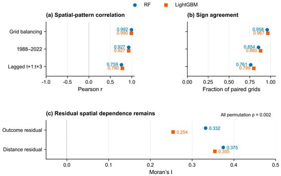
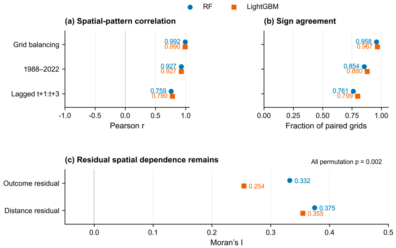
The fitted spatial ordering was more repeatable than the full regional sign pattern. Across 50 repeated spatial cross-fitting partitions with bandwidth reselection, the West–East difference was positive and the Eastern mean was negative in all fits. The Western mean was positive in 37 RF fits and 25 LightGBM fits; with k fixed at 75, both signs were retained in all 50 fits for each learner. Grid-balanced weighting, the higher-coverage period, and a strictly lagged response window also preserved much of the primary surface pattern (Figure 9; Table S4; Supplementary Figure S2; Section S12). These checks characterize stability under alternative implementations of the same data. Grid-mean first-stage nuisance residuals exhibited local spatial autocorrelation at the eight-nearest-neighbor scale: outcome and treatment residual Moran’s I values were 0.332 and 0.375 under RF and 0.254 and 0.355 under LightGBM (all permutation p = 0.002, the minimum attainable under 499 permutations; Figure 9c).
Figure 9.
Specification agreement and residual spatial dependence. (a) Pearson correlation and (b) sign agreement with the primary local surface under grid-balanced weighting, the 1988–2022 period, and the [t + 1, t + 3] window. (c) Moran’s I of grid-mean first-stage out-of-fold outcome and treatment residuals, using eight-nearest-neighbor weights and 499 permutations (all p = 0.002). These are residual diagnostics, not independent prediction scores.
Held-out spatial-block predictions did not show a consistent error reduction from the local model: RF improved slightly and LightGBM worsened slightly, with both paired MSE-difference intervals spanning zero (Supplementary Section S14). The local surfaces therefore describe adjusted spatial associations and do not establish an independent predictive gain.
First-stage out-of-fold nuisance diagnostics confirmed stable predictive fit and substantial remaining treatment variation across both learners and model branches (Supplementary Table S26). Across the 48,242 events (44 blocks in five spatial folds with zero block leakage), held-out outcome RMSE ranged from 0.4035 to 0.4074 (R2 = 0.2740–0.2880), treatment RMSE ranged from 0.8452 to 0.8655 (R2 = 0.2082–0.2449), and the residualized treatment standard deviation ranged from 0.8446 to 0.8650.
4. Discussion
4.1. Event-Scale Characteristics of Meteorological-to-Agricultural Drought Propagation
The event analysis identifies both the frequency and the timing of root-zone drought responses from an initially non-drought state. The 35.39% probability uses all eligible meteorological onsets as its denominator, while the lag distribution is conditional on the 17,072 successful responses. This distinction complements Yangtze studies based on index-phase relationships and matched drought episodes [6,7]: their propagation times and probabilities answer related questions but are not directly interchangeable with an onset-window estimate.
The predominance of lag 1–2 among successful responses supports continued root-zone monitoring after meteorological onset. Antecedent water storage can contribute to delayed soil-moisture depletion [3,12]. The root-zone product also smooths and delays surface observations through its filtering method [24,25], so physical soil-water memory and processing-induced persistence are combined in the observed lag distribution. Our paired comparison with ERA5-Land across 43,029 common onsets provides two key insights: first, nearly half of propagating events in ERA5-Land (49.48%, and 23.28% of all eligible onsets) also exhibited a 1–2 month delay, indicating that lagged root-zone response is not solely a satellite-filtering artifact; second, the 8.61-percentage-point higher delayed share in ESA CCI relative to ERA5-Land (58.09% versus 49.48%) demonstrates that exact lag proportions are sensitive to product-specific filtering and land-surface parameterization, and resolving their exact vadose-zone travel times requires independent multi-depth root-zone observations.
4.2. Spatial and Temporal Changes in Propagation
The primary event series shows higher propagation probabilities in the 2000s and 2010s than in the preceding periods, alongside a positive annual trend. This broad temporal change is consistent with evidence that propagation risk in the Yangtze has evolved over recent decades [9], although the datasets and definitions differ. Our low value for 2020–2022 and the sensitivity of full-period significance to the SSI reference period show that the evolution is not captured by a single uniform increase. Attribution of that change to warming, rainfall, or water management requires information beyond the trend analysis.
Autumn onsets had a higher propagation probability than those in the other seasons. Seasonal differences can reflect the balance between replenishment and depletion of soil water, but the event statistics alone do not identify individual atmospheric or agricultural drivers. The close agreement between the full-period and higher-coverage spatial maps suggests that the principal geographical pattern is not confined to the sparsely observed early years. Because these periods overlap, this comparison describes coverage sensitivity rather than independent temporal validation.
4.3. Regional Hydrological Context of Reservoir-Proximity Associations
The nonsignificant basin-wide DML coefficients and the contrasting local GWR surfaces describe complementary levels of covariate-adjusted spatial association. At the outset, we emphasize that because straight-line reservoir proximity does not measure water releases, canal connectivity, or irrigation scheduling, these coefficients reflect adjusted geographical associations within regional landscapes rather than causal effects of water-management operations. A constant coefficient summarizes the residual relationship across all events, whereas GWR allows the relationship to vary across neighborhoods. Cross-learner surface agreement (r = 0.799; Figure 10) and bandwidth invariance (k = 50–100; r = 0.960–0.983) support the broad fitted West–East spatial pattern, while the regional tests specify its tiered inferential reach: conditional fixed-residual tests reject spatial homogeneity (p = 0.040), direct three-region interaction models are significant under LightGBM (p = 0.0498) but not RF (p = 0.8062), and full-process spatial-block resampling yields marginal p-values (p = 0.100 and 0.090).
Figure 10.
Cross-learner correspondence of the fitted local reservoir-distance coefficients across the 1147 cropland grids. Each point is one grid; the horizontal and vertical axes give the Random Forest- and LightGBM-residualized local coefficients in percentage points per one standard deviation of log-distance. Colors identify the Western (<105° E; n = 235), transition (105–112° E; n = 449), and Eastern (≥112° E; n = 463) sectors. The dashed line is the 1:1 line and the solid lines mark zero. Pearson r = 0.799, and the sign agrees at 89.5% of the grids.
Distance to a dam also distinguishes landscape settings, and those settings differ by region. The observed elevation, slope, cropland, and river-discharge gradients provide a hydrological context for interpreting the fitted signs (Table 6; Figure 8c–e). Geographic proximity is a marker of where cropland and large reservoirs occur within the drainage landscape, alongside any influence of managed water.
In the West, cropland near large dams was lower, gentler, and more concentrated than cropland in the far-distance group. This is consistent with a transition from valley or basin-floor farming toward higher and steeper terrain. The fitted local means were positive, but the unadjusted group probabilities did not increase monotonically with distance, and the near-minus-far interval crossed zero. The small near group (19 grids in seven blocks) therefore supports a description of environmental setting more clearly than a claim of reservoir-related drought mitigation.
In the East, increasing dam distance instead corresponded to lower elevation, gentler slopes, more extensive cropland, and larger natural river discharge. Far-distance grids had lower propagation probability, placing the negative local coefficients in a landscape gradient from hill margins toward lowland river and lake settings. River access, groundwater exchange, and managed diversions could contribute to moisture persistence in such settings, but their individual contributions were not measured. The observed gradient helps interpret proximity without demonstrating a reservoir-operation mechanism.
These contextual differences also matter for adjustment. Elevation and slope were included among the 17 controls, whereas natural river discharge, canal connectivity, groundwater conditions, and actual releases were not. Flexible nuisance models can account for relationships represented in the measured controls; they cannot ensure that all spatially structured influences are removed [16,43]. The remaining local association should therefore be interpreted together with the regional environment rather than assigned entirely to dam regulation.
4.4. What the Spatial Analyses Establish
The spatial analysis separates surface stability from uncertainty in regional contrasts. Repeated cross-fitting preserved the regional ordering, but bandwidth reselection reduced the consistency of a positive Western mean. Fixed-residual tests condition on one nuisance fit and bandwidth; full-process resampling propagates both sources of variation. Their different results show why map agreement and conditional significance should be reported alongside the wider uncertainty of the full procedure (Figure 9). Furthermore, the significant eight-nearest-neighbor Moran’s I in grid-mean first-stage residuals (p = 0.002) underscores why random cross-fitting is inappropriate for hydro-climatic grids and motivates our 2° × 2° (~200 km) spatial-block design. Because 2° blocks are substantially larger than the eight-nearest-neighbor grid spacing (~25–50 km), block-clustered standard errors and block-level resampling absorb short-range within-block spatial autocorrelation. Nevertheless, if residual spatial dependence extends across adjacent 2° block boundaries, asymptotic cluster-robust intervals can remain mildly anti-conservative, and comparisons spanning a finite number of blocks (such as the 29 blocks supporting the direct West–East contrast, where small-sample df adjustment shifts LightGBM Holm p from 0.0498 to 0.0552) warrant cautious, multi-tier interpretation.
4.5. Limitations
The local fitting step does not by itself identify reservoir-operation effects. The reservoir models estimate retrospective, covariate-adjusted associations with geographic dam proximity rather than causal effects of reservoir operations. Duration and minimum SPEI contain full-spell information, the 355-reservoir inventory represents large dams rather than all storage and diversion infrastructure, and flexible machine-learning adjustment for 17 measured covariates cannot rule out unmeasured spatial confounders [43]. Actual releases, irrigation connectivity, and groundwater observations would be needed to distinguish reservoir operations from other spatially structured influences. Furthermore, while our paired ERA5-Land comparison confirms that 1–2 month propagation lags persist in an independent reanalysis product, the future integration of dense, multi-depth in situ soil-moisture monitoring networks will be essential to fully separate physical vadose-zone travel times from product-specific filtering memory.
The 0.25° monthly analysis averages sub-grid terrain, crops, and water management. Complete response windows protected the event outcomes from end-of-record truncation, although 53 eligible meteorological spells extended to December 2022 and may have truncated full-spell covariates. Finer temporal observations and independently mapped water-delivery areas would help separate rapid soil-moisture responses from the roles of connected reservoirs and other water sources.
5. Conclusions
Across 1147 persistent cropland grids in the Yangtze River Basin, 35.39% of 48,242 eligible meteorological drought onsets during 1981–2022 were accompanied or followed by agricultural drought within the onset month and the next two months. Among the 17,072 successful propagation responses in the primary ESA CCI root-zone product, 56.33% first crossed the SSI threshold at lag 1 or 2. Paired comparison across 43,029 common events in ERA5-Land confirmed a substantial delayed share (49.48% of successful responses and 23.28% of all eligible onsets), indicating that 1–2 month response lags are not specific to the satellite product, even though the exact delayed percentage is partly influenced by satellite exponential-filtering persistence. Autumn onsets had the highest propagation probability. The primary annual series showed a positive trend, with its full-period significance sensitive to the SSI reference period.
Global DML estimated weak average reservoir-distance associations, with intervals spanning zero under both learners. Locally, fitted GWR surfaces agreed across learners (r = 0.799), across adaptive bandwidths k = 50–100 (r = 0.960–0.983), and across repeated spatial partitions with predominantly positive coefficients in the West and negative coefficients in the East. Statistical evidence for this regional contrast is tiered across uncertainty levels: a constant-coefficient restriction was rejected under conditional fixed-residual inference (Holm-adjusted p = 0.040), direct three-region interaction models were learner-dependent (p = 0.0498 under LightGBM and p = 0.8062 under RF), and conservative full-process spatial-block resampling—propagating both nuisance-estimation and bandwidth-selection uncertainty—yielded marginal p-values for the West–East mean contrast (p = 0.100 for RF and p = 0.090 for LightGBM).
The contrasting local associations coincided with different gradients in terrain, cropland, and natural river discharge, indicating that reservoir proximity represents covariate-adjusted spatial associations within regional hydro-environmental settings rather than causal effects of reservoir scheduling. The combination of onset-based event analysis and spatially blocked global and local modeling also provides an analytical approach that can be adapted to other regions with suitable hydro-climatic and infrastructure data while accounting for the spatial heterogeneity and context dependence of drought propagation relationships.
Supplementary Materials
The following supporting information can be downloaded at: https://www.mdpi.com/article/10.3390/w18222884/s1, The accompanying supplementary material contains Figures S1–S4, Tables S1–S27, and Sections S1–S19, covering data coverage, event windows, model settings, bandwidth sensitivity, soil-moisture product sensitivity, held-out nuisance diagnostics, trend sensitivity, direct regional contrasts, conditional and full-process resampling, distance-group profiles, and outer-block prediction checks.
Author Contributions
Conceptualization, J.Z. and Y.Y.; Methodology, J.Z.; Software, J.Z.; Validation, L.Z. and P.L.; Formal analysis, J.Z.; Resources, R.L.; Data curation, J.Z., L.Z. and P.L.; Writing—original draft preparation, J.Z.; Writing—review and editing, J.Z., L.Z., P.L., Y.Y., R.L. and S.W.; Visualization, J.Z.; Supervision, Y.Y., R.L. and S.W.; Project administration, Y.Y. All authors have read and agreed to the published version of the manuscript.
Funding
This work was supported by the New Generation Artificial Intelligence-National Science and Technology Major Project (grant 2026ZD0126204), the Fundamental Research Funds for the Central Universities (grant 226-2025-00069, 226-2025-00223).
Data Availability Statement
The input datasets are publicly available from the providers listed in Table 1 and the References. The derived event-level table and the analysis code are available from the corresponding author on reasonable request.
Acknowledgments
We thank the providers of the public environmental datasets used in this study. During the preparation of this manuscript, the authors used ChatGPT (GPT-6 Astra, OpenAI) for the purposes of language editing and checking Python code as described in Section 2.6. The authors have reviewed and edited the output and take full responsibility for the content of this publication. This work was also supported by the Deep-time Digital Earth (DDE) Big Science Program and the Earth System Big Data Platform of the School of Earth Sciences, Zhejiang University.
Conflicts of Interest
The authors declare no conflicts of interest.
References
- Mishra, A.K.; Singh, V.P. A review of drought concepts. J. Hydrol. 2010, 391, 202–216. [Google Scholar] [CrossRef] [Scilit]
- Dai, A. Drought under global warming: A review. WIREs Clim. Change 2011, 2, 45–65. [Google Scholar] [CrossRef] [Scilit]
- Zhang, X.; Hao, Z.; Singh, V.P.; Zhang, Y.; Feng, S.; Xu, Y.; Hao, F. Drought propagation under global warming: Characteristics, approaches, processes, and controlling factors. Sci. Total Environ. 2022, 838, 156021. [Google Scholar] [CrossRef] [Scilit] [PubMed]
- Van Loon, A.F. Hydrological drought explained. WIREs Water 2015, 2, 359–392. [Google Scholar] [CrossRef] [Scilit]
- Vicente-Serrano, S.M.; Beguería, S.; López-Moreno, J.I. A Multiscalar Drought Index Sensitive to Global Warming: The Standardized Precipitation Evapotranspiration Index. J. Clim. 2010, 23, 1696–1718. [Google Scholar] [CrossRef] [Scilit]
- Li, R.; Chen, N.; Zhang, X.; Zeng, L.; Wang, X.; Tang, S.; Li, D.; Niyogi, D. Quantitative analysis of agricultural drought propagation process in the Yangtze River Basin by using cross wavelet analysis and spatial autocorrelation. Agric. For. Meteorol. 2020, 280, 107809. [Google Scholar] [CrossRef] [Scilit]
- Xu, Z.; Wu, Z.; Shao, Q.; He, H.; Guo, X. From meteorological to agricultural drought: Propagation time and probabilistic linkages. J. Hydrol. Reg. Stud. 2023, 46, 101329. [Google Scholar] [CrossRef] [Scilit]
- Um, M.J.; Kim, Y.; Jung, K.; Lee, M.; An, H.; Min, I.; Kwak, J.; Park, D. Evaluation of drought propagations with multiple indices in the Yangtze River basin. J. Environ. Manag. 2022, 317, 115494. [Google Scholar] [CrossRef] [Scilit] [PubMed]
- Hu, R.; Yuan, S.; Jin, J.; Zhu, L.; Liu, Y. Long-term changes in the drought propagation characteristics in the Yangtze River Basin. J. Hydrol. Reg. Stud. 2026, 63, 103014. [Google Scholar] [CrossRef] [Scilit]
- Barker, L.J.; Hannaford, J.; Chiverton, A.; Svensson, C. From meteorological to hydrological drought using standardised indicators. Hydrol. Earth Syst. Sci. 2016, 20, 2483–2505. [Google Scholar] [CrossRef] [Scilit]
- Seneviratne, S.I.; Corti, T.; Davin, E.L.; Hirschi, M.; Jaeger, E.B.; Lehner, I.; Orlowsky, B.; Teuling, A.J. Investigating soil moisture–climate interactions in a changing climate: A review. Earth-Sci. Rev. 2010, 99, 125–161. [Google Scholar] [CrossRef] [Scilit]
- Gupta, A.; Karthikeyan, L. Role of Initial Conditions and Meteorological Drought in Soil Moisture Drought Propagation: An Event-Based Causal Analysis Over South Asia. Earth’s Future 2024, 12, e2024EF004674. [Google Scholar] [CrossRef] [Scilit]
- Van Loon, A.F.; Gleeson, T.; Clark, J.; Van Dijk, A.I.J.M.; Stahl, K.; Hannaford, J.; Di Baldassarre, G.; Teuling, A.J.; Tallaksen, L.M.; Uijlenhoet, R.; et al. Drought in the Anthropocene. Nat. Geosci. 2016, 9, 89–91. [Google Scholar] [CrossRef] [Scilit]
- Xing, Z.; Ma, M.; Zhang, X.; Leng, G.; Su, Z.; Lv, J.; Yu, Z.; Yi, P. Altered drought propagation under the influence of reservoir regulation. J. Hydrol. 2021, 603, 127049. [Google Scholar] [CrossRef] [Scilit]
- Huang, S.; Zhang, X.; Chen, N.; Li, B.; Ma, H.; Xu, L.; Li, R.; Niyogi, D. Drought propagation modification after the construction of the Three Gorges Dam in the Yangtze River Basin. J. Hydrol. 2021, 603, 127138. [Google Scholar] [CrossRef] [Scilit]
- Chernozhukov, V.; Chetverikov, D.; Demirer, M.; Duflo, E.; Hansen, C.; Newey, W.; Robins, J. Double/debiased machine learning for treatment and structural parameters. Econom. J. 2018, 21, C1–C68. [Google Scholar] [CrossRef] [Scilit]
- Roberts, D.R.; Bahn, V.; Ciuti, S.; Boyce, M.S.; Elith, J.; Guillera-Arroita, G.; Hauenstein, S.; Lahoz-Monfort, J.J.; Schröder, B.; Thuiller, W.; et al. Cross-validation strategies for data with temporal, spatial, hierarchical, or phylogenetic structure. Ecography 2017, 40, 913–929. [Google Scholar] [CrossRef] [Scilit]
- Valavi, R.; Elith, J.; Lahoz-Monfort, J.J.; Guillera-Arroita, G. blockCV: An R package for generating spatially or environmentally separated folds for k-fold cross-validation of species distribution models. Methods Ecol. Evol. 2019, 10, 225–232. [Google Scholar] [CrossRef] [Scilit]
- Brunsdon, C.; Fotheringham, A.S.; Charlton, M.E. Geographically Weighted Regression: A Method for Exploring Spatial Nonstationarity. Geogr. Anal. 1996, 28, 281–298. [Google Scholar] [CrossRef] [Scilit]
- Fotheringham, A.S.; Charlton, M.E.; Brunsdon, C. Geographically Weighted Regression: A Natural Evolution of the Expansion Method for Spatial Data Analysis. Environ. Plan. A 1998, 30, 1905–1927. [Google Scholar] [CrossRef] [Scilit]
- Zhang, Q.; Miao, C.; Su, J.; Gou, J.; Hu, J.; Zhao, X.; Xu, Y. A new high-resolution multi-drought-index dataset for mainland China. Earth Syst. Sci. Data 2025, 17, 837–853. [Google Scholar] [CrossRef] [Scilit]
- Zhang, Q.; Miao, C. CHM_Drought: A New High-Resolution Multi-Drought Indices Dataset for Mainland China; Version 1.0; Zenodo: Geneva, Switzerland, 2025. [Google Scholar] [CrossRef]
- Gruber, A.; Scanlon, T.; van der Schalie, R.; Wagner, W.; Dorigo, W. Evolution of the ESA CCI Soil Moisture climate data records and their underlying merging methodology. Earth Syst. Sci. Data 2019, 11, 717–739. [Google Scholar] [CrossRef] [Scilit]
- Lems, J.; Preimesberger, W.; Dorigo, W.A. ESA CCI SM RZSM Long-Term Climate Data Record of Root-Zone Soil Moisture from Merged Multi-Satellite Observations; Version 9.2; TU Wien: Vienna, Austria, 2025. [Google Scholar] [CrossRef]
- Pasik, A.; Gruber, A.; Preimesberger, W.; De Santis, D.; Dorigo, W. Uncertainty estimation for a new exponential-filter-based long-term root-zone soil moisture dataset from Copernicus Climate Change Service (C3S) surface observations. Geosci. Model Dev. 2023, 16, 4957–4976. [Google Scholar] [CrossRef] [Scilit]
- AghaKouchak, A. A baseline probabilistic drought forecasting framework using standardized soil moisture index: Application to the 2012 United States drought. Hydrol. Earth Syst. Sci. 2014, 18, 2485–2492. [Google Scholar] [CrossRef] [Scilit]
- Yang, J.; Huang, X. The 30 m annual land cover dataset and its dynamics in China from 1990 to 2019. Earth Syst. Sci. Data 2021, 13, 3907–3925. [Google Scholar] [CrossRef] [Scilit]
- Yang, J.; Huang, X. The 30 m Annual Land Cover Datasets and Its Dynamics in China from 1985 to 2025; Version 1.0.5; Zenodo: Geneva, Switzerland, 2026. [Google Scholar] [CrossRef]
- Muñoz-Sabater, J.; Dutra, E.; Agustí-Panareda, A.; Albergel, C.; Arduini, G.; Balsamo, G.; Boussetta, S.; Choulga, M.; Harrigan, S.; Hersbach, H.; et al. ERA5-Land: A state-of-the-art global reanalysis dataset for land applications. Earth Syst. Sci. Data 2021, 13, 4349–4383. [Google Scholar] [CrossRef] [Scilit]
- ISRIC—World Soil Information. SoilGrids Layers. Available online: https://docs.isric.org/globaldata/soilgrids/SoilGrids_faqs_01.html (accessed on 16 October 2026).
- Yamazaki, D.; Ikeshima, D.; Sosa, J.; Bates, P.D.; Allen, G.H.; Pavelsky, T.M. MERIT Hydro: A High-Resolution Global Hydrography Map Based on Latest Topography Dataset. Water Resour. Res. 2019, 55, 5053–5073. [Google Scholar] [CrossRef] [Scilit]
- Lehner, B.; Grill, G. Global river hydrography and network routing: Baseline data and new approaches to study the world’s large river systems. Hydrol. Process. 2013, 27, 2171–2186. [Google Scholar] [CrossRef] [Scilit]
- Lehner, B.; Verdin, K.; Jarvis, A. New Global Hydrography Derived From Spaceborne Elevation Data. Eos Trans. AGU 2008, 89, 93–94. [Google Scholar] [CrossRef] [Scilit]
- Hu, J.; Miao, C.; Su, J.; Zhang, Q.; Gou, J.; Sun, Q. An upgraded high-precision gridded precipitation dataset for the Chinese mainland considering spatial autocorrelation and covariates. Earth Syst. Sci. Data 2025, 17, 3987–4004. [Google Scholar] [CrossRef] [Scilit]
- Li, X.; Wang, K.; Jiang, H.; Wang, G.; Yu, J.; Luo, Q.; Liu, X. China Large rEservoirs Attributes and DRainage Boundaries (CLEAR) Dataset; Version 1.2; Figshare: London, UK, 2026. [Google Scholar] [CrossRef]
- Mann, H.B. Nonparametric Tests Against Trend. Econometrica 1945, 13, 245–259. [Google Scholar] [CrossRef] [Scilit]
- Sen, P.K. Estimates of the Regression Coefficient Based on Kendall’s Tau. J. Am. Stat. Assoc. 1968, 63, 1379–1389. [Google Scholar] [CrossRef]
- Hamed, K.H.; Rao, A.R. A modified Mann-Kendall trend test for autocorrelated data. J. Hydrol. 1998, 204, 182–196. [Google Scholar] [CrossRef] [Scilit]
- Breiman, L. Random Forests. Mach. Learn. 2001, 45, 5–32. [Google Scholar] [CrossRef] [Scilit]
- Ke, G.; Meng, Q.; Finley, T.; Wang, T.; Chen, W.; Ma, W.; Ye, Q.; Liu, T.Y. LightGBM: A Highly Efficient Gradient Boosting Decision Tree. In Proceedings of the 31st International Conference on Neural Information Processing Systems (NIPS 2017), Long Beach, CA, USA, 4–9 December 2017; Curran Associates, Inc.: Red Hook, NY, USA, 2017; Volume 30, pp. 3146–3154. Available online: https://proceedings.neurips.cc/paper_files/paper/2017/hash/6449f44a102fde848669bdd9eb6b76fa-Abstract.html (accessed on 16 October 2026).
- Nie, X.; Wager, S. Quasi-oracle estimation of heterogeneous treatment effects. Biometrika 2021, 108, 299–319. [Google Scholar] [CrossRef] [Scilit]
- Holm, S. A Simple Sequentially Rejective Multiple Test Procedure. Scand. J. Stat. 1979, 6, 65–70. [Google Scholar] [CrossRef]
- Reich, B.J.; Yang, S.; Guan, Y.; Giffin, A.B.; Miller, M.J.; Rappold, A. A Review of Spatial Causal Inference Methods for Environmental and Epidemiological Applications. Int. Stat. Rev. 2021, 89, 605–634. [Google Scholar] [CrossRef] [Scilit] [PubMed]

Disclaimer/Publisher’s Note: The statements, opinions and data contained in all publications are solely those of the individual author(s) and contributor(s) and not of MDPI and/or the editor(s). MDPI and/or the editor(s) disclaim responsibility for any injury to people or property resulting from any ideas, methods, instructions or products referred to in the content. |
© 2026 by the authors. Licensee MDPI, Basel, Switzerland. This article is an open access article distributed under the terms and conditions of the Creative Commons Attribution (CC BY) license.