


Abstract
The increasing integration of variable renewable energy (VRE) into power grids has significantly widened the peak-to-valley difference in net load and intensified its volatility. To follow these rapid load changes, cascade hydropower plants must frequently adjust their output, operate within unstable oscillation zones, or undergo repeated start-stop cycles. This creates a growing conflict between the system’s demand for peak shaving and the actual operational capabilities of hydropower plants. To address this challenge, this paper proposes a method for reconstructing the load curve based on fuzzy recognition of peak-valley characteristics. By adaptively adjusting the number of identified features, the method transforms the highly fluctuating net load into a multi-segment linear form. This preserves essential peak and valley information while promoting output stability. Building on this reconstructed load curve, a short-term peak-shaving model for cascade hydropower is developed, aiming to minimize the standard deviation of the residual load. The model is solved using an improved progressive optimality algorithm (POA) that integrates feasible region reduction with a multi-segment, variable-step-size search strategy. The peak-shaving performance is evaluated under three VRE penetration scenarios: low (10%), medium (20%), and high (40%). A case study conducted on China’s Wujiang River demonstrates the effectiveness of the proposed method. The load curve reconstruction transforms hydropower output from hourly sawtooth-like fluctuations into a stepwise pattern, albeit with a slight reduction in the peak-to-valley difference optimization rate (PVOR). For example, in the 10% penetration scenario, the frequency of output adjustments decreases by 73.2%. As the VRE penetration rate increases, the net peak-to-valley load difference grows sharply, and the PVOR of the reconstruction scheme declines from 26.70% to 9.12%. Nevertheless, the frequency of output adjustments does not exceed 15 times, thereby maintaining stable operation. The proposed approach achieves a reasonable trade-off between peak-shaving effectiveness and operational stability, offering a practical solution for hydropower dispatch in grids with high VRE penetration rates.
1. Introduction
The rapid expansion of variable renewable energy (VRE), particularly wind and solar power, is fundamentally transforming modern power systems and playing an increasingly vital role in supporting the global low-carbon transition [1,2]. In China, for instance, total installed wind and solar capacity exceeded 1840 GW by the end of 2025 and is expected to reach approximately 2200 GW by 2030 [3,4]. As a result, wind and solar generation is quickly evolving from a supplementary energy source into the primary contributor to electricity supply [5]. However, the inherent randomness, volatility, intermittency, and anti-peaking characteristics of these sources place significant stress on both power balance and frequency regulation. Consequently, the traditional dispatch paradigm, which simply follows the electricity load curve, is no longer adequate [6,7,8].
As the share of wind and solar power continues to grow, the net load curve, defined as the original load minus wind and solar output [9], has shifted from a conventional single-peak or double-peak pattern to a more complex multi-peak, multi-valley structure. This new profile is characterized by wider peak-to-valley differences, steeper ramping rates, and more frequent intraday fluctuations. Accordingly, the system’s demand for short-term flexible regulation capacity has risen sharply [10,11]. Hydropower is widely recognized as a core flexible regulation resource capable of smoothing fluctuations in VRE output [12,13]. However, under conditions of high VRE penetration, it faces a fundamental dilemma. On the one hand, hydropower plants must adjust their output more frequently and over a broader range to respond to net load variations [10,12]. On the other hand, such frequent adjustments force generating units to operate extensively in vibration zones and undergo repeated start-stop cycles, accelerating equipment wear and potentially compromising operational safety [14,15,16]. Striking an effective balance between peak-shaving performance and operational stability has thus become a critical challenge in the dispatch of cascade hydropower systems [17]. This challenge has been widely recognized in recent studies on pumped storage and hydropower units [18,19].
Extensive research has been conducted on the short-term peak-shaving dispatch of hydropower, both domestically and internationally. These studies can be broadly classified into two categories. The first category focuses on developing peak-shaving dispatch models and their corresponding solution algorithms. These studies typically aim to minimize a specific statistical characteristic of the grid’s residual load, such as minimizing the peak-to-valley difference [20], minimizing the variance of the residual load [21], or maximizing the peak-shaving energy [22]. A variety of optimization algorithms have been employed to determine the optimal operating points for hydropower units along the daily load curve, including the Progressive Optimality Algorithm (POA) [23], mixed-integer linear programming [24,25,26], and particle swarm optimization [27]. Over time, these models have progressively incorporated practical constraints such as ramping limits, hydraulic connections, and comprehensive reservoir utilization requirements [28,29]. In recent years, the scope of research has expanded from individual hydropower plants to large-scale cascaded reservoir systems, significantly increasing model scale and complexity. For instance, Zhao et al. [30] developed a decomposition-iteration approach tailored for large-scale cascade hydropower systems with N reservoirs and multiple stages. This method significantly reduces the computational complexity associated with high-dimensional optimization problems. Wang et al. [31] developed a short-term optimization model that balances peak-shaving demands across multiple power grids within a unified framework. Shen et al. [32] quantified the functional relationship between long-term power generation and short-term peak-shaving performance. Liu et al. [33] investigated a short-term operation method that leverages the flexibility of interprovincial transmission via high-voltage direct-current lines. Wu et al. [34] proposed a short-term load allocation model for mega-scale cascade hydropower plants that accounts for complex hydro-electric interconnections. It is worth noting that a parallel line of research has attempted to address the flexibility–stability trade-off directly within the dispatch or unit model. Zhang et al. [18] developed a soft-linking model that couples the power system unit commitment model with the pump-turbine governing system model, and Zhao et al. [19] established a nonlinear model of pumped hydro energy storage systems to evaluate stability and efficiency under flexible operation. These studies provide valuable insights into the coordination of flexibility and stability at the unit or system level. However, they require detailed unit-level parameters and stability indicators, and they do not modify the load-side tracking target.
Importantly, all of the above studies, whether they focus on dispatch optimization or unit-level flexibility–stability coordination, treat the original net load curve as the direct target for hydropower output to follow, using optimization algorithms to align generation as closely as possible with the load profile. This paradigm rests on a fundamental assumption: that the net load curve is the appropriate target for hydropower to faithfully track [11]. Before the large-scale integration of VRE, this assumption was reasonable, as the net load curve was relatively smooth and the required frequency of output adjustments remained manageable. However, as the penetration rate of VRE increases, the high-frequency fluctuation component of the net load curve grows substantially, causing the cost of precise tracking to rise sharply. Research indicates that while optimization algorithms can theoretically yield optimal solutions, they often require frequent and drastic adjustments to hydropower output that are difficult to implement in actual operation [35,36,37]. In contrast, the present study addresses the same challenge from a load-side perspective: by reconstructing the net load curve before dispatch, the tracking target itself becomes smoother and more stable, which reduces the frequency of output adjustments without altering the dispatch or unit model.
The second category of research addresses load preprocessing or output smoothing strategies. In terms of load preprocessing, some studies extract typical load scenarios through cluster analysis or apply curve-fitting methods to smooth the load profile [38,39]. However, these approaches are primarily used for load forecasting or generating representative scenarios; they have not yet been integrated into a closed-loop system with the dispatch optimization model, limiting their ability to directly support dispatch decisions. Regarding output smoothing, other studies have introduced output stability constraints [40] or smoothness penalty terms [29] into the dispatch model to suppress sharp fluctuations in hydropower output. Nevertheless, these methods typically treat smoothness as either a hard constraint or a fixed-weight penalty. They lack a systematic analysis of the quantitative trade-off between peak-shaving performance and the degree of smoothing, making it difficult to achieve adaptive coordination across different operating scenarios. Moreover, the aforementioned methods commonly use fixed time segments to define peak and valley load intervals, making them ill-suited to adapt to the dynamic shifts in net load shapes resulting from changing VRE penetration rates. Existing research shows that as VRE penetration rate increases, the primary peak period of net load may shift later, the secondary peak may occur earlier, and the main valley period may move from nighttime to midday [11,41]. In the face of these dynamic changes, fixed-interval methods appear inflexible and cannot effectively capture the time-varying characteristics of the load peak-valley structure. This leads to discrepancies between dispatch plans and actual peak-shaving requirements.
In summary, existing research exhibits several notable shortcomings in the coordinated optimization of peak-shaving performance and operational stability: (1) Load preprocessing and dispatch optimization are treated as separate processes, lacking an integrated framework to unify them. (2) There is insufficient systematic analysis of the quantitative trade-off between peak-shaving performance and output stability. (3) Peak and valley load identification relies on fixed time intervals, which cannot adaptively track the dynamic evolution of net load patterns. To overcome these shortcomings, this paper introduces a two-stage scheduling framework that prioritizes load curve reconstruction before proceeding to optimization. First, a load curve reconstruction method based on fuzzy recognition of peak-valley characteristics is introduced. This method detects peak and valley points using first-order differencing, clusters them using triangular membership functions, and ensures schedulability through minimum duration constraints. As a result, the net load is adaptively transformed into a simplified target curve in the form of a multi-segment line, hereafter referred to as the reconstructed load curve. Building on this reconstructed curve, a short-term peak-shaving model for cascade hydropower is developed, with the objective of minimizing the standard deviation of the residual load. An improved POA is designed, combining feasible region reduction with a multi-segment, variable-step-size search strategy. Through simulated dispatch of cascade hydropower, the peak-shaving performance of the proposed reconstruction method is systematically evaluated under typical scenarios and across different VRE penetration rates. This work provides theoretical support for the flexible dispatch of cascade hydropower and grid operation in the context of high VRE penetration.
2. Methods
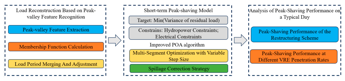
To address the challenge of accurately characterizing the dynamic evolution of peak-to-valley patterns in net load under high VRE penetration, this study proposes a load curve reconstruction method based on fuzzy recognition of peak-valley characteristics. A short-term peak-shaving dispatch model for cascade hydropower is then developed, balancing the grid’s peak-shaving requirements with the need for stable power plant output. The research is carried out in three stages, as illustrated in the overall methodology framework in Figure 1:
First, a net load curve reconstruction method based on fuzzy recognition of peak-valley characteristics is proposed. Fuzzy recognition techniques are employed to extract the peak and valley characteristics of the load curve. A reconstruction model specifically designed for cascade hydropower peak-shaving is established, providing accurate load boundary conditions for subsequent dispatch optimization.
Second, a short-term peak-shaving dispatch model for cascade hydropower systems is developed, along with an improved POA for solving it. Based on the reconstructed load curve, the model aims to minimize the standard deviation of the residual load while comprehensively considering output stability constraints. The POA is enhanced by incorporating a sequential load-shedding method and a dynamic iterative search strategy for available generation intervals, enabling simultaneous optimization of peak-shaving performance and output stability.
Third, simulation experiments are carried out on cascade hydropower dispatch to compare the performance of the reconstruction-based approach with that of the non-reconstruction approach. The evolution of peak-shaving performance under varying penetration rates of VRE is also examined. The effectiveness of the proposed two-stage scheduling framework, which prioritizes load curve reconstruction before optimization, is validated from two perspectives: peak-shaving performance and output stability.
The model implementation and computational environment were as follows: all numerical simulations and optimization calculations were mainly performed using Java 1.8.0_31 (Oracle Corporation, Austin, TX, USA) in the IntelliJ IDEA Community Edition 2024.2.4 environment (JetBrains s.r.o., Prague, Czech Republic), with MATLAB R2024a (MathWorks, Natick, MA, USA) used as an auxiliary tool. The data plots were generated using OriginPro 2026b (OriginLab Corporation, Northampton, MA, USA). The flowcharts were drawn and the final figures were assembled using Microsoft PowerPoint for Microsoft 365 (Microsoft Corporation, Redmond, WA, USA). The tables were prepared and formatted using Microsoft Excel for Microsoft 365 (Microsoft Corporation, Redmond, WA, USA).
Figure 1.
Methodology framework.
2.1. Load Curve Reconstruction Based on Fuzzy Recognition of Peak-Valley Characteristics
When a high proportion of VRE is connected to the grid, the volatility of the net load increases significantly, and the peak-to-valley difference widens considerably. If this raw net load is used directly as the load boundary for peak-shaving and load-balancing dispatch of cascade hydropower, hydropower plants would be forced to respond to every minor fluctuation. This would cause generating units to frequently enter vibration zones or undergo repeated start-stop cycles, thereby worsening grid frequency deviations. To address this issue, this study proposes a method for reconstructing the net load curve based on fuzzy recognition of peak-valley characteristics. For net load sequences that exhibit distinct peak and valley features, fuzzy recognition techniques are employed to extract their underlying patterns. By combining mathematical analysis with statistical characteristics, the method identifies the peak and valley features of the load curve. The original continuous curve, characterized by severe fluctuations, is then transformed into a reconstructed load curve in the form of a multi-segment line. This process eliminates small-amplitude, high-frequency fluctuations while preserving key peak and valley information. As a result, a clear and stable load boundary is provided for subsequent peak-shaving dispatch.
2.1.1. Peak-Valley Feature Extraction
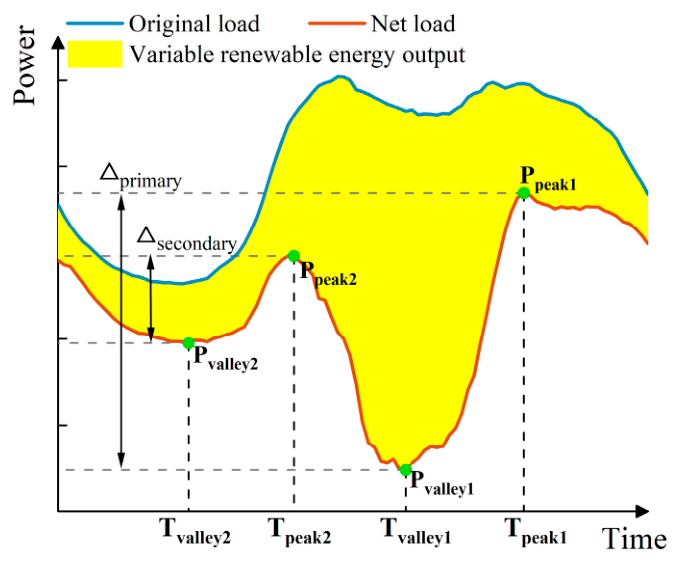
To accurately identify the key turning points of the net load curve, this study employs the first-order difference method, combined with bidirectional sign-change constraints, to detect local maxima and minima in the net load sequence [42]. This method effectively filters out noise and pseudo-peaks or valleys by requiring that the slope changes direction at the detected point. To further refine the results, two criteria are applied: a minimum duration constraint ΔTmin ensures that detected peaks or valleys last for a sufficient period, preventing the identification of transient fluctuations as significant features, and a dynamic amplitude threshold δ = μ ± 2σ filters out small amplitude fluctuations by setting a threshold based on the mean μ and standard deviation σ of the load data. When multiple potential peaks or valleys are identified, the optimal points are selected by evaluating the residual change relative to the reconstructed curve (see Figure 2). Specifically, the relative peak-to-valley ratio Rpv is defined to quantify the contribution of secondary peak-valley fluctuations to the overall peak-to-valley difference:
where Δprimary is the primary peak-to-valley difference (MW); Δsecondary is the secondary peak-to-valley difference (MW). The primary and secondary peaks, Ppeak1 and Ppeak2 correspond to the maximum and second-largest load values identified after sorting all detected peaks in descending order (MW). Similarly, the primary and secondary valleys, Pvalley1 and Pvalley2 represent the minimum and second-smallest load values obtained after sorting all detected valleys in ascending order (MW). Tpeak1, Tvalley1, Tpeak2 and Tvalley2 are the times at which the primary peak, primary valley, secondary peak, and secondary valley occur, respectively.
Figure 2.
Schematic representation of grid load dynamics.
2.1.2. Membership Function Calculation
To fully capture the double-peak, double-valley characteristics of the net load, the model constructs a four-order feature space consisting of the primary peak, secondary peak, primary valley, and secondary valley. This enables a four-dimensional dynamic representation of the load curve. Specifically, as illustrated in Figure 3, an adaptive triangular membership function [43] is employed to map the load sequence point by point. The function is defined by three parameters: the left boundary a, the peak b and the right boundary c. By calculating the membership vector of each point with respect to the four-order features, a nonlinear relationship between feature intensity and load points is established. The parameters of the membership functions for the primary peak and primary valley are jointly determined by amplitude thresholds and time windows. The parameters for the secondary peak and secondary valley are calibrated with the objective of minimizing reconstruction residuals.
Figure 3.
Triangular membership function based on peak and valley attributes: (a) Identification of the primary peak. (b) Identification of remaining points. (c) Identification of the primary valley.
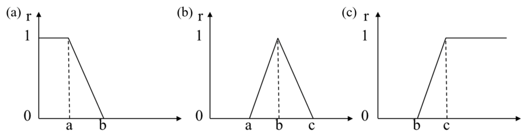
Calculate the membership vector for each net load PNL,t at period t:
where μpeak1, μpeak2, μvalley1 and μvalley2 represent the membership degrees of net load PNL,t at period t for the primary peak, secondary peak, primary valley, and secondary valley, respectively.
The initial label for each point is determined based on the highest membership degree. It is important to note that as the penetration rate of VRE increases, the peak-to-valley difference in net load gradually widens, while the relative ratio of the peak-to-valley difference Rpv steadily decreases. Consequently, the importance of the secondary peak-to-valley difference relative to the power system’s peak-shaving requirements diminishes. When the relative ratio of the peak-to-valley difference Rpv falls below a certain threshold, fuzzy recognition based on the relational characteristics of the four attributes can no longer accurately capture the overall peak-valley behavior. In such cases, the fluctuations associated with the secondary peak and secondary valley can be treated as a flat segment. Consequently, the set of four characteristic attributes consisting of the primary peak, primary valley, secondary peak, and secondary valley is reduced to three: primary peak, primary valley, and flat segment. This simplification enables the power system’s regulation resources to concentrate on adjusting the overall peak-to-valley difference of the regulation curve, thereby achieving optimal overall peak-shaving performance.
Based on the fluctuation trends in the load curve, the number of feature attributes can be adaptively adjusted. For example, when there is a significant gap between the primary peak and the secondary peak and the curve is relatively flat, transition points can be added between the primary and secondary peaks. The same principle applies to the primary valley and the secondary valley. Adding transition points improves the accuracy with which the reconstructed curve captures load fluctuation characteristics and reduces the peak-shaving requirements imposed on other power sources.
2.1.3. Load Period Merging and Adjustment
Based on the membership degree calculations of the aforementioned feature values, each point on the load curve is clustered according to its proximity to the peak and valley characteristics, thereby achieving an adaptive segmentation of the load curve. However, to prevent frequent oscillations between adjacent points and ensure the smoothness of the reconstructed load, a minimum interval constraint is introduced: the duration of any consecutive segment sharing the same label must not fall below a specified threshold ΔTmin. Using the time intervals between feature points as state variables, points that do not satisfy the minimum duration requirement are reassigned with the objective of minimizing the residual error within that period.
where PNL,t represents the net load at period t (MW); represents the optimized load value (MW) at period t; s and e are the start and end times, respectively, of the time periods to be merged.
For each merged feature segment, the average net load within the segment is used as the reconstructed load value.
where represents the load value (MW) of the combined feature segment.
Based on the principles described above, the load curve reconstruction process proceeds as follows. First, the load curve to be reconstructed and the minimum duration constraint are input. After smoothing and normalization using a Gaussian filter [44], the peak and valley points are identified using a first-order difference method. The number of feature attributes is then adaptively determined based on the relative peak-to-valley difference. Initial feature labels are obtained through point-by-point mapping using a triangular membership function. Subsequently, merging and adjustment are performed with the objectives of satisfying the minimum duration constraint and minimizing the residual within each segment. Finally, the reconstructed load curve is output. The detailed process is illustrated in Figure 4.
Figure 4.
Flowchart of the load curve reconstruction method.
Several key parameters are involved in this process, and their selection is based on physical considerations and operational practice. The Gaussian filter parameters are chosen to effectively suppress high-frequency noise in the net load profile while preserving its dominant temporal features, consistent with common signal processing practice for power system data. The minimum segment length is set to reflect the typical minimum continuous operation requirement for hydropower units, ensuring mechanical safety and avoiding excessive start-stop cycles. The amplitude and gradient thresholds for transition segments are determined to capture realistic ramping capabilities between adjacent peak and valley segments. The relative peak-valley difference threshold governs the switching between different feature-number patterns, where a larger relative difference indicates a more pronounced peak-valley structure that warrants finer segmentation. The effectiveness of these parameter choices is further validated through the sensitivity analysis in Section 4.3.3, which confirms the rationality of these parameter choices and the robustness of the reconstruction method.
2.2. Short-Term Peak-Shaving Model
This study develops a short-term peak-shaving dispatch model for cascade hydropower plants that simultaneously considers both the grid’s peak-shaving requirements and the plants’ stable operation characteristics. The model is designed to determine the optimal peak-shaving strategy for cascade hydropower plants under scenarios characterized by highly fluctuating net load.
2.2.1. Objective Functions
This study aims to minimize the standard deviation of the residual grid load after hydropower peak-shaving. The objective is to enable cascade hydropower plants to smooth out net load fluctuations and reduce the peak-to-valley difference. The objective function is expressed as follows:
where t is the time slot index; N is the total number of scheduling periods; i is the cascade hydropower plant index; M is the total number of hydropower plants; Pres,t is the residual grid load (MW) for period t after accounting for hydroelectric peak-shaving; Phydro,t is the total output (MW) of the cascade hydropower plants at period t; is the output (MW) of hydropower plant i at period t; PNL,t represents the net load at period t (MW); PLoad,t represents the original load at period t (MW); PWind,t represents the wind power output at period t (MW); PPV,t represents the photovoltaic output at period t (MW).
Pres,t = PNL,t − Phydro,t
PNL,t = PLoad,t − PWind,t − PPV,t
The power output of each hydropower plant in the model is calculated as follows:
where Ki is the comprehensive output coefficient of hydropower plant i (see Table 1); is the generation flow of hydropower plant i at period t (m3/s); is the generating head of plant i at period t (m); is the reservoir water level of hydropower plant i at period t (m), obtained by interpolation from the storage-water level relationship curve; is the tailwater level of hydropower plant i at period t (m), determined from the tailwater-discharge relationship curve based on the released flow.
Table 1.
Characteristics of cascade hydropower plants in the Wujiang River Basin.
2.2.2. Constraints
The model must satisfy the following constraints: water balance, hydraulic connectivity, upper and lower limits on power generation flow, upper and lower limits on outflow, upper and lower limits on storage volume, upper and lower limits on output, water level fluctuation limits, initial and final storage volume requirements, and the short-term ramping capacity of the hydropower plant. These constraints are specified as follows:
- (1)
- Water balance constraints
- (2)
- Hydraulic connection constraints
- (3)
- Upper and lower limits on power generation flow
- (4)
- Upper and lower limits of generating head
- (5)
- Upper and lower limits on outflow
Qi,min ≤ Qi,t ≤ Qi,max
- (6)
- Upper and lower bound constraints on storage volume
Vi,min ≤ Vi,t ≤ Vi,max
- (7)
- Upper and lower output constraints
- (8)
- Water level variation constraints
|Zi,t − Zi,t−1| ≤ ΔZi
- (9)
- Initial and final storage volume constraints
- (10)
- Ramping capability limits
As shown in Equations (9), (10) and (15), the model adopts a simplified power–flow relationship in which a comprehensive output coefficient Ki is used, while head variation and tailwater effects are dynamically updated at each time step through the storage–water level curve and the tailwater level–flow curve. The maximum and minimum head constraints are explicitly enforced. However, unit-efficiency curves, vibration zones, and minimum start–stop times are not explicitly represented at the plant level. This simplification is acceptable for short-term peak-shaving dispatch at the plant level because the reconstructed load curve and the minimum duration constraint indirectly reduce the risk of frequent start–stop cycles and prolonged operation in vibration zones. These unit-level characteristics should be considered in subsequent unit-level load allocation to further ensure practical implementability.
2.2.3. Solution Algorithm
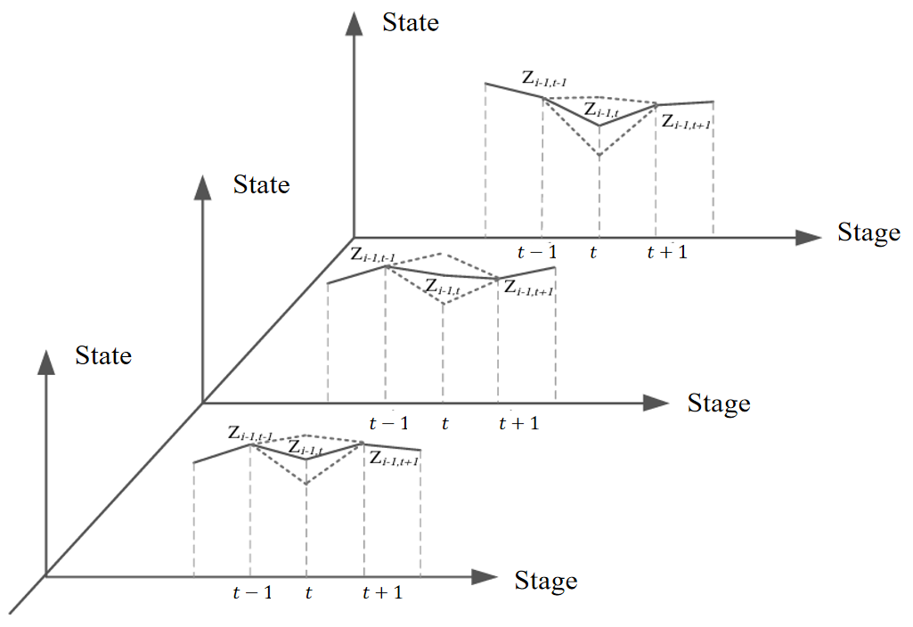
POA decomposes multi-stage decision problems into a series of two-stage subproblems that are solved iteratively, as illustrated in Figure 5. It offers several advantages, including no need for discrete state variables, low memory requirements, monotonic convergence, and a continuous and feasible optimization trajectory. As a result, POA is widely used in the short-term scheduling of cascade hydropower plants [45,46]. Accordingly, this paper selects POA as the basic solution algorithm. However, the standard POA still has limitations when applied to this problem, including strong dependence on the initial solution, high computational complexity for per-time-step optimization, difficulty in ensuring output stability, and limited capability in handling water spillage. To address these limitations, this paper proposes improvements in four areas: feasible region reduction, initial solution acquisition, optimization method, and spillage correction.
- (1)
- Feasible region reduction
Infeasible state combinations are eliminated through dual constraints. Forward and backward recursion are performed from the beginning and end of the scheduling period, respectively, based on the upper and lower limits of outflow. The intersection of the two feasible storage volume trajectories for each time step is taken as the compressed upper and lower bounds of storage volume. Additionally, after determining the storage volume at the end of a given time step, the feasible range for the storage volume at the beginning of that time step is further narrowed based on outflow and water level variation constraints.
- (2)
- Obtaining the initial solution
The sequential load-shedding method [47] is used to obtain a high-quality initial solution. Dispatch priorities are determined based on the regulation capacity of each reservoir. The power output process is determined on a time-step-by-time-step basis, starting from the time step with the maximum residual load. Iterative adjustments are then made using the water level at the end of the dispatch period as the control objective.
- (3)
- Multi-segment optimization with variable step size
This approach treats the transition periods between adjacent stable segments as the optimization target and performs joint optimization on a multi-segment basis. This avoids the computational redundancy associated with optimizing each segment individually. At the same time, an exponential decay coefficient is introduced to dynamically adjust the calculation step size. Large step sizes are used in the early stages of iteration to rapidly traverse the solution space, and the step size is gradually reduced in later stages to converge to the optimal solution:
where α is the exponential decay coefficient, which controls the rate at which the step size decreases; δk is the step size during phase k.
δk+1 = α ⋅ δk(α ∈ (0,1))
Figure 5.
Schematic diagram of the progressive optimality algorithm (POA) optimization process. The solid lines represent the initial trajectory, and the dashed lines represent the updated trajectory during the iterative optimization.
- (4)
- Spillage correction strategy
When spillage occurs due to cascade hydropower coupling, a pre-release method is adopted. This involves increasing the output of the optimization segment preceding the hydropower plant experiencing spillage, while simultaneously reducing the output of the current optimization segment of the hydropower plant immediately upstream. This reduces downstream inflow. Water level constraints are verified iteratively until the spillage is eliminated or the constraint limits are reached.
Based on the improvements described above, the detailed solution process and corresponding flowchart (Figure 6) are presented as follows:
Figure 6.
Flowchart of the short-term peak-shaving dispatch model. The dashed boxes represent the detailed sub-modules corresponding to each main step.
Step 1: Input grid load, wind and solar output processes, and cascade hydropower runoff data. Set the number of dispatch periods and the maximum number of iterations.
Step 2: Use the sequential load-shedding method to obtain the cascade hydropower output process, which serves as the initial trajectory for POA optimization.
Step 3: Using the multi-segment, variable-step-size optimization method, first determine the time intervals during which the output of the hydropower plant changes. Then, fix the reservoir storage at the start of the optimization segment Vstate and the reservoir storage at the end of the optimization segment Vstate+2. Next, apply the feasible region reduction method to identify all feasible combinations of the reservoir storage at the intermediate time step Vstate+1. For each feasible combination, calculate the mean square deviation of the residual load.
Step 4: Select the scenario with the smallest mean square deviation to update the reservoir storage process. If spillage occurs, adjust the solution according to the correction strategy.
Step 5: Perform rolling calculations until all time periods have been optimized. Determine whether the maximum number of iterations has been reached and output the optimal results.
3. Case Study
3.1. Study Area
This study focuses on the Wujiang River Basin in Guizhou Province, located in southwestern China. Within this basin, eleven large and medium-sized hydropower plants have been constructed. To highlight the peak-shaving characteristics of cascade operations, seven hydropower plants were selected for this study: Hongjiadu (HJD), Dongfeng (DF), Suofengying (SFY), Wujiangdu (WJD), Goupitan (GPT), Silin (SL), and Shatuo (ST), as illustrated in Figure 7 [11]. The total installed capacity of these seven hydropower plants is 8315 MW. Among them, HJD is a multi-year regulation reservoir. GPT possesses multi-year regulation capability when operated in conjunction with upstream reservoirs. DF and WJD are seasonal regulation reservoirs, while the remaining hydropower plants are daily regulation reservoirs. The main characteristic parameters of the cascade hydropower system are presented in Table 1.
Figure 7.
Geographic distribution of hydropower plants in the Wujiang River Basin, Southwest China. Reprinted from Renewable Energy, Vol. 267, Zhehua Liu, Qiaofeng Tan, Rong Huang, Zhenni Wang, Xin Wen, Short-term peak-shaving strategies for cascade hydropower against evolving net load in systems with high VRE penetration, 125773, Copyright (2026), with permission from Elsevier. (License Number: 502097583.)
With the diversification of its power generation mix, Guizhou Province in China has gradually developed a synergistic and complementary structure comprising hydropower, thermal power, wind power, and solar power. By the end of 2025, the total installed capacity of Guizhou’s power system reached 87.31 GW. Of this, hydropower accounted for 17.62 GW, while wind and solar power together accounted for 37.39 GW. Hydropower represented approximately 20% of the total installed capacity, and wind and solar power accounted for about 42% [48]. Looking ahead, wind and solar installed capacity is projected to increase to 75.00 GW by 2030 and further rise to 105.00 GW by 2035. As wind and solar power gradually become the dominant sources of electricity supply in the region, this will place even greater demands on the flexibility of the Wujiang River cascade hydropower system.
3.2. Data Sources and Scenario Settings
The 2023 measured data used in this study include the 15-min load and wind/solar output data recorded by the Guizhou Provincial Power Grid Dispatch Center, and the inflow data recorded by hydropower stations in the Wujiang River basin. Since only daily average inflow data are available, the daily average inflow is assumed to be constant within each day and applied to all 96 time steps. This simplification is acceptable because peak regulation primarily occurs during the dry season, during which runoff remains relatively stable throughout the day.
The 2030 dataset was constructed as follows: First, the load series was obtained by proportionally scaling the 2023 15-min load series to match the projected total social electricity consumption of Guizhou Province. Second, the wind and solar output series were calculated by multiplying the projected installed capacity by the corresponding time-varying capacity factor. Finally, the net load series was computed by subtracting wind and solar output from load at each 15-min interval.
The year 2030 is selected as the baseline year for the following reasons. It marks the end of Guizhou Province’s 15th Five-Year Plan period and serves as a critical milestone in the province’s medium- to long-term energy transition. By that time, the installed capacity of wind and solar power is expected to increase substantially relative to current levels. As a result, this baseline year provides a representative basis for capturing the structural evolution of net load patterns under a scenario characterized by a high penetration of VRE. Accordingly, actual operational data under typical meteorological conditions were selected to correspond to three penetration rate scenarios: low (10%), medium (20%), and high (40%).
4. Results and Discussion
4.1. Analysis of Net Load Pattern Evolution
Figure 8 presents a comparison of typical net load curves under different VRE penetration rates. As the penetration rate increases from 10% to 40%, the net load curve undergoes a systematic evolution from a uniform double-peak pattern to a single-peak, deep-valley pattern. At a penetration rate of 10%, the net load exhibits a typical double-peak, double-valley structure. The morning and evening peak amplitudes are roughly symmetrical, and the primary valley occurs between 3:00 a.m. and 7:00 a.m. The overall shape closely resembles traditional load characteristics. When the penetration rate rises to 20%, the morning peak decreases by approximately 9–10 GW compared to the 10% scenario, while the evening peak remains largely unchanged, breaking the symmetry of the double-peak pattern. At the same time, high midday photovoltaic generation causes the midday valley to fall below the nighttime valley, shifting the primary valley from nighttime to midday. The system’s temporal characteristics begin to be dominated by VRE output. At a penetration rate of 40%, the morning peak virtually disappears, and the evening peak becomes the dominant peak. During certain midday periods, net load even turns negative. The load curve evolves from a double-peak, double-valley pattern to a single-peak, deep-valley pattern, and the system’s operational logic shifts from passive generation adjustment to meet load demand toward coordinated interaction between generation and load.
Figure 8.
Comparison of typical net load curves under different penetration rates.
These results indicate that, as the penetration rate increases, the peak structure of the net load evolves from a double-peak pattern to one dominated by the evening peak. Meanwhile, the valley structure transitions from a shallow valley in the early morning to a deep valley at midday, which may even reach negative values. For hydropower regulation, it is no longer appropriate to allocate output evenly according to the conventional double-peak load profile. Instead, efforts must be directed toward strengthening the capacity to support the evening peak and enhancing the ability to rapidly regulate and absorb load during midday hours. This reflects a shift from broad time-window peak shaving to precise response during critical peak periods.
4.2. Verification of Load Reconstruction Results
In the hydropower bases of Southwest China, the role of hydropower systems differs significantly between the wet and dry seasons. During the wet season, abundant inflows drive hydropower plants to operate primarily for energy generation, leaving limited flexibility for peak-shaving. In contrast, during the dry season, reduced inflows allow hydropower to fully exploit its regulation flexibility, making it the primary resource for grid peak-shaving. Consequently, the dry season represents the most critical scenario for validating the effectiveness of the proposed load reconstruction strategy. The selected day (1 January) also falls within the winter heating period, when the net load profile—shaped by the combined effects of heating demand and high nighttime wind output—exhibits a large peak-to-valley difference and steep ramp rates. This represents a relatively extreme condition within the dry season and allows for a more rigorous test of the method’s adaptability under demanding operating conditions.
Using the original load and VRE output data from the Guizhou power grid on 1 January 2030, and applying fuzzy recognition of peak-valley characteristics, the net load curve was categorized at each data point. This process transformed the highly fluctuating net load profile into a multi-segment curve with distinct segment characteristics, as shown in Figure 9. On a typical dry season day, both the raw load and the net load exhibit significant intraday fluctuations. The peak-to-valley difference for the raw load is approximately 19.55 GW, while that for the net load is approximately 18.91 GW, with the absolute value narrowing slightly. However, the superimposition of VRE output results in more frequent peak-to-valley transitions and more pronounced local sharp rises and falls in net load. The net load curve rapidly switches between high levels in the morning and evening and low levels at midday, exhibiting strong step-like and abrupt change characteristics. These features place higher demands on both the ramping capacity of hydropower and the precision of dispatch. The reconstructed curve retains the primary temporal trends of the original net load while categorizing the intraday process into characteristic segments, such as the primary peak, secondary peak, primary valley, and secondary valley, each with a duration of no less than 2 h. This approach not only satisfies the minimum duration constraint to ensure the physical feasibility of dispatch instructions and equipment adjustments but also more clearly highlights key inflection points and adjustment priorities. This facilitates targeted responses by flexible resources, such as hydropower, based on these characteristic segments.
Figure 9.
Reconstructed net load curve based on fuzzy recognition under a typical scenario.
4.3. Analysis of Peak-Shaving Performance on a Typical Day
To reveal the impact of load reconstruction on hydropower peak-shaving dispatch behavior and verify the practical effectiveness of the proposed fuzzy recognition of peak-valley characteristics method in reducing hydropower regulation pressure and improving dispatch feasibility, two comparative scenarios were established:
Scenario 1 (Baseline Scenario): The net load curve is directly used as the tracking target, and hydropower output strictly follows the continuous fluctuations of the net load.
Scenario 2 (Restructuring Scenario): The net load curve first undergoes fuzzy recognition and reconstruction of its peak-valley characteristics, converting it into a multi-segment line. This reconstructed curve is then used as the tracking target for hydropower dispatch.
4.3.1. Peak-Shaving Performance of the Restructuring Scheme
To ensure that the subsequent peak-shaving comparison mainly reflects the effect of load reconstruction rather than the choice of solution algorithm, both schemes are solved using the improved POA. The reliability and efficiency of the improved POA are first verified against the standard POA under the same initial solution and computing environment. The improved POA converges in 10 iterations and 11.56 s, compared with 50 iterations and 203.92 s for the standard POA, while achieving a comparable residual load standard deviation (4922 MW vs. 4935 MW). This improvement is attributed to four modifications: feasible region reduction, sequential load-shedding initialization, multi-segment variable-step-size search, and spillage correction. These results confirm that the improved POA is computationally efficient and converges reliably for short-term peak-shaving dispatch of large-scale cascade hydropower systems.
Using this validated algorithm, the scheduling performance of the two schemes is compared in Figure 10 and Table 2. Under Scheme 2, the frequency of output adjustments is 11, representing a 73.2% reduction compared to the 41 adjustments required under Scheme 1. The restructuring strategy transforms frequent, time-step-by-step fine-tuning into a limited number of phased adjustments. As shown in Figure 10, Scheme 1 exhibits high-frequency, sawtooth-like fluctuations on a per-time-slot basis, whereas Scheme 2 displays a step-like output profile over larger time scales, such as the output plateaus observed in time slots 40–44 and 72–83. In terms of peak-to-valley difference optimization rate (PVOR), Scheme 2 achieves 26.70%, a decrease of 15.18 percentage points compared to Scheme 1’s 41.88%. The restructuring strategy sacrifices some of the PVOR to enable hydropower output to exhibit modularity and coordination over larger time scales, thereby enhancing output stability and engineering feasibility. Furthermore, the total power generation of the cascade under Scheme 1 and Scheme 2 is 51.43 GWh and 63.35 GWh, respectively, with the restructured scenario being approximately 23% higher. This indicates that the restructuring strategy improves output stability without sacrificing power generation efficiency.
Figure 10.
Comparison of dispatch processes at a 10% variable renewable energy (VRE) penetration rate: (a) Scenario 1; (b) Scenario 2.
Table 2.
Comparison of peak-shaving performance at different VRE penetration rates.
4.3.2. Peak-Shaving Performance at Different VRE Penetration Rates
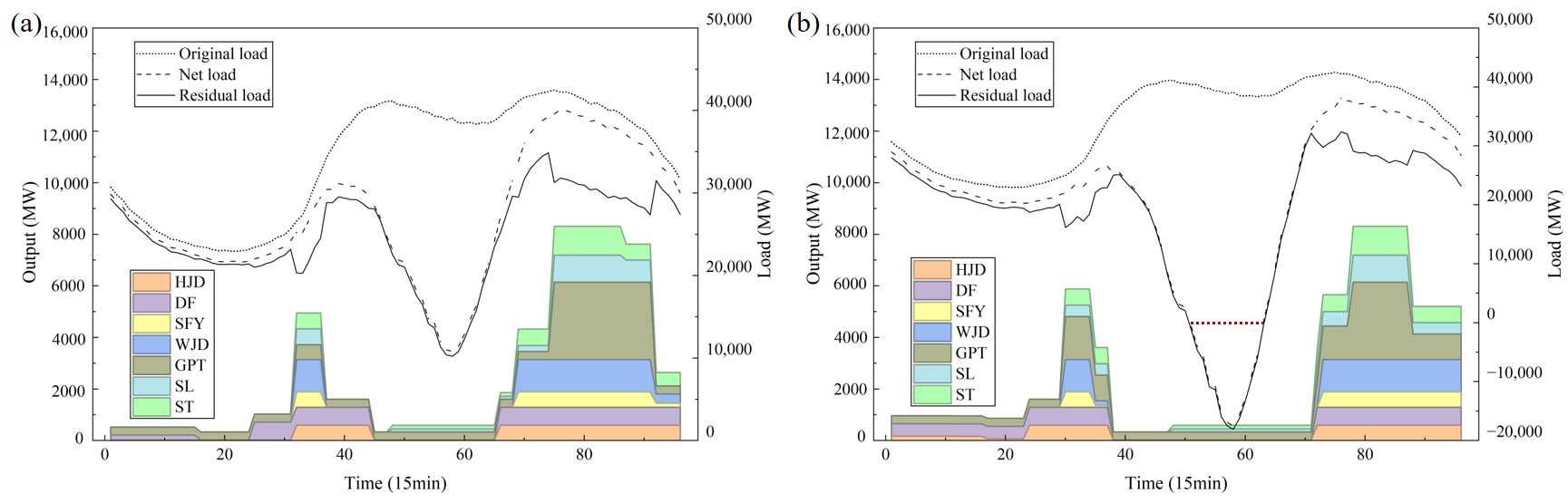
To reveal the evolutionary characteristics of hydropower dispatch under different VRE penetration rates, a scenario with 10% VRE penetration was used as the baseline to compare and analyze performance differences at penetration rates of 20% and 40%. The relevant indicator data are presented in Table 2. In terms of the frequency of output adjustments, Scheme 1 recorded 41, 47, and 54 adjustments at penetration rates of 10%, 20%, and 40%, respectively, with the frequency increasing continuously as the penetration rate rose. This reflects that, under the non-reconstruction scheme, cascade hydropower is forced to respond to net load fluctuations at a higher frequency. Scheme 2 recorded 11 adjustments at both 10% and 20% penetration rates and 15 adjustments at 40%. The frequency remained consistent at low and medium penetration rates but rose slightly at the high penetration rate. This is because the emergence of negative net load during midday forces hydropower to complete larger-scale output adjustments within a shorter timeframe, as illustrated in Figure 11. In terms of PVOR, at a penetration rate of 10%, Scheme 1 achieved 41.88% while Scheme 2 achieved 26.70%. At a penetration rate of 20%, Scheme 1 dropped to 26.92% and Scheme 2 to 15.80%. At a penetration rate of 40%, Scheme 1 further dropped to 14.22% and Scheme 2 to 9.12%. As the penetration rate increases, the net peak-to-valley load difference rises significantly, and the PVOR decreases accordingly. This indicates that under high-penetration scenarios, the system’s peak-shaving demand surges, while hydropower’s relative contribution to peak-shaving declines, requiring greater coordination among additional peak-shaving resources. In addition to PVOR and adjustment frequency, Table 2 also reports the total hydropower generation, curtailment rate, spillage rate, and ecological flow satisfaction rate. These indicators are further discussed below.
Figure 11.
Comparison of hydropower dispatch processes: (a) 20% VRE penetration rate; (b) 40% VRE penetration rate. The red dashed line represents the zero-load baseline, indicating the periods of negative net load during midday.
While the above indicators demonstrate the peak-shaving performance under different VRE penetration rates, it is equally important to verify whether the reconstruction strategy compromises reservoir operation, generation, and ecological requirements. These aspects are examined below.
To examine whether the reconstruction strategy compromises reservoir operation, Figure 12 and Figure 13 present the reservoir water level trajectories of the seven hydropower plants under the non-reconstruction scheme (Scheme 1) and the reconstruction scheme (Scheme 2), respectively, at 10%, 20%, and 40% VRE penetration rates. All water levels remain within the allowable upper and lower bounds, and the water level fluctuation constraints are satisfied in both schemes and all scenarios. As the penetration rate increases, the water level fluctuations become more pronounced, reflecting the greater regulation burden placed on hydropower. Comparing the two schemes, the reconstruction scheme exhibits slightly smoother water level variations, particularly at 40% penetration, where the midday and evening fluctuations are less abrupt than those under the non-reconstruction scheme. These results confirm that the reconstructed load curve does not push the reservoirs beyond their operational limits, and it helps to reduce the frequency and magnitude of water level adjustments.
Figure 12.
Reservoir water level trajectories of the seven hydropower plants under the non-reconstruction scheme (Scheme 1) at 10%, 20%, and 40% VRE penetration rates. Subplots (a–g) correspond to HJD, DF, SFY, WJD, GPT, SL, and ST, respectively. The blue solid, orange dashed, and green dotted lines represent 10%, 20%, and 40% VRE penetration rates, respectively.
Figure 13.
Reservoir water level trajectories of the seven hydropower plants under the reconstruction scheme (Scheme 2) at 10%, 20%, and 40% VRE penetration rates. The layout and line styles are the same as in Figure 12.
Table 2 shows that at 10% VRE penetration, Scheme 2 produces 63.35 GWh of hydropower on the typical day, approximately 23.2% more than the 51.43 GWh of Scheme 1. At 20% and 40% penetration, Scheme 2 generates 62.52 and 62.72 GWh, respectively, compared with 62.62 and 65.93 GWh for Scheme 1; the reductions relative to Scheme 1 are below 5%. The wind and solar curtailment rate is 0% at 10% and 20% penetration under both schemes, but reaches 10.1% at 40% penetration under Scheme 2, slightly higher than the 9.8% under Scheme 1. No spillage occurs in any case, and the ecological flow satisfaction rate remains 100% in all cases. This indicates that the smoothing of hydropower output is achieved at a small cost of additional curtailment because the flattened midday net-load profile limits hydropower’s ability to absorb surplus generation. The release processes and ecological flow requirements are explicitly enforced as constraints in the model, and all scenarios satisfy the minimum ecological flow and water supply requirements. Taken together, these results indicate that the reconstruction strategy achieves a better balance between peak-shaving performance and operational stability without violating reservoir safety or ecological constraints.
It should be noted that this study is conducted at the plant level, and unit-level indicators such as time spent in vibration zones and start-stop counts are not explicitly modeled. The value of 15 adjustments is not a pre-defined threshold; it is the result obtained by the reconstructed scheme under the 40% VRE penetration scenario in this case study, compared with 54 adjustments under the non-reconstructed scheme. This comparison demonstrates the effectiveness of load reconstruction in smoothing hydropower output and reducing adjustment frequency. However, the smoother hydropower output does not eliminate the short-term fluctuations in the residual load; rather, it may shift them to other resources, such as thermal units, storage, and demand response. Quantifying this system-level consequence is beyond the scope of the present study, which focuses on the hydropower side. Therefore, the conclusions drawn here are limited to hydropower dispatch, and the system-level effects require further investigation. Future work will extend the model to the unit level by incorporating unit efficiency curves, vibration zone constraints, and minimum start-stop times and develop system-level coordination frameworks to evaluate the shift of fluctuations to other resources.
4.3.3. Parameter Sensitivity Analysis
The baseline parameters are selected based on physical considerations and operational practice, as described in Section 2.1.3. To further verify their rationality, a one-at-a-time sensitivity analysis was conducted based on the net load data of 96 points per day for the entire year of 2030. All evaluation metrics in Table 3 are annual averages of the daily values over 2030. The parameters examined include the Gaussian filter parameter, the minimum duration constraint, the amplitude threshold, and the relative peak-to-valley ratio threshold, which governs the switching between four-feature and three-feature patterns (i.e., feature-number switching). The evaluation metrics include the reconstruction RMSE, the average number of segments, and the main peak-valley retention rate. The reconstruction RMSE measures the deviation between the reconstructed curve and the original net load; the average number of segments reflects the smoothness of the reconstructed curve; and the main peak-valley retention rate indicates the ability to preserve the dominant peak-valley structure. The baseline parameters are: Gaussian filter σ = 2, minimum duration ΔTmin = 2 h, amplitude threshold = 2.0σ, and Rpv threshold = 0.3. The parameter ranges and results are shown in Table 3. Overall, the minimum duration constraint has the most significant effect on the reconstruction, the amplitude threshold has no influence within the tested range, and the Gaussian filter parameter and the Rpv threshold have minor effects.
Table 3.
Sensitivity analysis of the load curve reconstruction parameters.
As shown in Table 3, the minimum duration constraint ΔTmin plays a decisive role in the smoothness and fidelity of the reconstructed curve. As ΔTmin increases from 1 h to 4 h, the average number of segments decreases from 11.18 to 5.32, while the reconstruction RMSE increases from 3602 MW to 10,548 MW. This indicates that a longer minimum segment length makes the reconstructed curve smoother but deviates more from the original curve. Notably, when ΔTmin reaches 4 h, the main peak-valley retention rate drops sharply to 45.55%, indicating that an excessively long minimum duration constraint over-smooths the curve and destroys the dominant peak-valley structure, making the reconstructed curve unable to reflect the key features of the original net load. When ΔTmin = 1 h, the retention rate is the highest (90.00%), but the average number of segments is 11.18, meaning the curve still contains considerable fluctuations and is not conducive to reducing the frequency of hydropower output adjustments. Considering the trade-off, ΔTmin =2 h achieves a balanced performance, with an average of 7.24 segments, a reconstruction RMSE of 8041 MW, and a retention rate of 87.44%. Therefore, it is selected as the baseline value.
The amplitude threshold has no influence on the reconstruction within the range of 1.0σ to 3.0σ, and all metrics remain identical. This is because a fallback mechanism is adopted in the dynamic amplitude filtering: when the number of retained peaks or valleys is less than two, the algorithm reverts to the original extremum list, thereby ensuring the stability of feature identification. In this case, all three values trigger the same fallback path, so the reconstructed curve remains unchanged. The Gaussian filter parameter σ and the Rpv threshold have minor effects on the reconstruction. When σ varies from 1 to 3, the reconstruction RMSE ranges from 7495 to 8041 MW, the average number of segments ranges from 7.24 to 7.47, and the retention rate ranges from 87.37% to 88.04%. When Rpv threshold varies from 0.1 to 0.4, the reconstruction RMSE ranges from 6827 to 8111 MW, the average number of segments ranges from 7.15 to 8.04, and the retention rate ranges from 86.98% to 88.65%. These variations are all within 5%, indicating that the reconstruction is not sensitive to these two parameters and that the baseline values are within a reasonable range. In summary, the baseline parameter combination achieves a good balance among curve smoothness, fitting accuracy, and feature preservation. The sensitivity analysis confirms the rationality of the parameter selection and demonstrates the robustness of the proposed reconstruction method within reasonable parameter ranges.
5. Conclusions
This paper addresses the inherent trade-off between peak-shaving performance and operational stability in cascade hydropower dispatch under scenarios with high VRE integration. To resolve this conflict, a two-stage scheduling framework is proposed, in which load curve reconstruction is performed prior to optimization. Using 2030 as the baseline year and selecting data from typical meteorological days, three scenarios with low (10%), medium (20%), and high (40%) VRE penetration rates are established to systematically validate the effectiveness of the proposed method. The main conclusions are as follows:
- (1)
- The proposed load curve reconstruction method, based on fuzzy recognition of peak-valley characteristics, detects peak and valley points through first-order differencing, employs triangular membership function clustering, and ensures schedulability via a minimum duration constraint. This method can adaptively transform the original net load into a simplified target curve in the form of a multi-segment line, thereby seamlessly integrating load preprocessing with scheduling optimization. It can adaptively switch feature spaces in response to changes in penetration rates, overcoming the limitation of fixed time-period divisions that cannot track the dynamic evolution of net load patterns. This approach transforms hydropower scheduling from tracking every individual fluctuation to responding to structural peaks and valleys, significantly reducing the complexity and randomness of scheduling decisions.
- (2)
- The reconstruction method transforms hydropower output from hourly sawtooth fluctuations to a stepped distribution, at the cost of sacrificing some of the PVOR. Taking the 10% penetration scenario as an example, the PVOR of the reconstructed scheme is 26.70%, which is approximately 15 percentage points lower than the 41.88% achieved by the non-reconstructed scheme. However, the frequency of output adjustments decreases from 41 to 11, a reduction of 73.2%. This indicates that while the reconstruction strategy sacrifices some peak-to-valley difference optimization efficiency, it significantly reduces the frequency of output adjustments, thereby enhancing the feasibility of the dispatch plan.
- (3)
- As the penetration rate of VRE increases, the net load profile evolves from a double-peak, double-valley pattern to a single-peak pattern accompanied by a deepened valley, leading to greater peak-shaving pressure. At a penetration rate of 10%, the reconstruction strategy achieves a PVOR of 26.70% with 11 output adjustments. When the penetration rate reaches 40%, the optimization rate decreases to 9.12%. This decline is attributed to the sharp rise in the baseline peak-to-valley difference of the net load as the penetration rate increases. Meanwhile, the frequency of output adjustments increases only slightly to 15, thereby preserving output stability. These findings indicate that higher VRE penetration further amplifies the advantage of the reconstruction strategy, which maintains acceptable output stability at a relatively low peak-shaving cost.
These findings suggest that hydropower dispatch under high VRE penetration should shift its focus from precisely following the raw net load curve to tracking a reconstructed load curve that retains essential peak-valley information. Such a shift requires dispatch protocols to incorporate minimum duration requirements and adapt peak-valley feature identification as VRE penetration and load shapes evolve. Performance evaluation should also be broadened from a single peak-shaving index to stability-oriented metrics such as adjustment frequency, ramp rate, and time spent in vibration zones. In high-penetration systems, hydropower should be coordinated with storage, demand response, and thermal units, and the reconstructed curve should be updated in a rolling manner using day-ahead forecasts. These measures would help dispatch centers achieve a practical balance between peak-shaving effectiveness and operational stability. However, the present study addresses short-term peak-shaving dispatch at the plant level, where the reconstructed load curve serves as the tracking target for cascade hydropower. Extending this framework to the unit level by incorporating unit efficiency characteristics and operating constraints and to the system level by coordinating hydropower with storage, demand response, and thermal units would further translate the load-side reconstruction idea into a practical dispatch paradigm for high-VRE power systems.
Author Contributions
Conceptualization, J.H.; methodology, J.H.; software, Y.W.; writing—original draft preparation, X.Z.; writing—review and editing, Y.H.; visualization, T.Z.; supervision, Y.C.; project administration, Q.T. All authors have read and agreed to the published version of the manuscript.
Funding
This research was funded by the National Natural Science Foundation of China (grant number 52479013) and the Basic Research Program of Jiangsu (grant number BK20251481).
Data Availability Statement
The data presented in this study are available upon request from the corresponding author due to commercial restrictions.
Conflicts of Interest
Authors Jin Hou, Xi Zhu, Yashan He, Tijian Zeng and Yu Chen were employed by the company Guizhou Wujiang Hydropower Development Co., Ltd., Guiyang, 550002, China. The remaining authors declare that the research was conducted in the absence of any commercial or financial relationships that could be construed as a potential conflict of interest.
Abbreviations
The following abbreviations are used in this manuscript:
| VRE | variable renewable energy |
| POA | Progressive Optimality Algorithm |
| PVOR | peak-to-valley difference optimization rate |
| Rpv | relative peak-to-valley ratio |
| Δprimary | primary peak-to-valley difference |
| Δsecondary | secondary peak-to-valley difference |
| Ppeak1 | maximum load value identified after sorting all detected peaks in descending order |
| Ppeak2 | second-largest load value identified after sorting all detected peaks in descending order |
| Pvalley1 | minimum load value obtained after sorting all detected valleys in ascending order |
| Pvalley2 | second-smallest load value obtained after sorting all detected valleys in ascending order |
| Tpeak1 | time at which the primary peak occurs |
| Tvalley1 | time at which the primary valley occurs |
| Tpeak2 | time at which the secondary peak occurs |
| Tvalley2 | time at which the secondary valley occurs |
| μpeak1 | membership degree of load point for the primary peak |
| μpeak2 | membership degree of load point for the secondary peak |
| μvalley1 | membership degree of load point for the primary valley |
| μvalley2 | membership degree of load point for the secondary valley |
| PNL,t | net load at period t |
| optimized load value at period t | |
| s | start time of the time periods to be merged |
| e | end time of the time periods to be merged |
| load value of the combined feature segment | |
| Pres,t | residual grid load for period t after accounting for hydroelectric peak-shaving |
| Phydro,t | total output of the cascade hydropower plants at period t |
| output of hydropower plant i at period t | |
| PLoad,t | original load at period t |
| PWind,t | wind power output at period t |
| PPV,t | photovoltaic output at period t |
| Ki | comprehensive output coefficient of hydropower plant i |
| power generation flow rate of the hydropower plant i at period t | |
| generating head of plant i at period t | |
| reservoir water level of hydropower plant i at period t, obtained by interpolation from the storage-water level relationship curve | |
| tailwater level of hydropower plant i at period t, determined from the tailwater-discharge relationship curve based on the released flow | |
| Vi,t | reservoir storage volume of the hydropower plant i at period t |
| Qi,t | total outflow rate of hydropower plant i at period t, which is the sum of the power generation flow and the spillage flow |
| power generation flow rate of hydropower plant i at period t | |
| spillage flow rate of hydropower plant i at period t | |
| Ii,t | inflow rate into the reservoir of the hydropower plant i at period t |
| basin runoff at the hydropower plant i + 1 at period t | |
| Φi +1 | set of upstream reservoirs that have a direct hydraulic relationship with the hydropower plant i + 1 at level |
| power generation flow rate of the hydropower plant i at period t | |
| maximum allowable power generation diversion flow rate of the hydropower plant i | |
| Hi,min | minimum generating head of hydropower plant i at period t |
| maximum generating head of hydropower plant i at period t | |
| Qi,min | minimum outflow rate required for the hydropower plant i to meet comprehensive downstream water use needs, such as ecological, navigation, and water supply |
| Qi,max | maximum allowable outflow rate for a hydropower plant i that meets flood control requirements |
| Vi,min | dead storage volume of hydropower plant i |
| Vi,max | maximum allowable storage volume of hydropower plant i, which corresponds to the flood control restriction level during the flood season and the normal storage level during all other periods |
| minimum output of hydropower plant i, which is generally the plant’s forced output | |
| maximum output of hydropower plant i, which is generally the plant’s installed capacity | |
| ΔZi | maximum water level variation between adjacent time periods at the i-th power plant |
| Vi,1 | the reservoir storage volume of the hydropower plant i at the beginning of the scheduling period |
| Vi,T+1 | the reservoir storage volume of the hydropower plant i at the end of the scheduling period |
| specified reservoir storage volume of the hydropower plant i at the beginning of the scheduling period | |
| specified reservoir storage volume of the hydropower plant i at the end of the scheduling period | |
| Ri | maximum ramping rate of hydropower plant i |
| α | exponential decay coefficient, which controls the rate at which the step size decreases |
| δk | step size during the phase k |
References
- Thapa, S.; Magee, T.; Zagona, E. Factors That Affect Hydropower Flexibility. Water 2022, 14, 2563. [Google Scholar] [CrossRef] [Scilit]
- Agarwal, A.; Sharma, T. Integrated Energy System Modeling Perspectives for Future Decarbonization Pathways Based on Sector Coupling, Life-Cycle Emissions and Vehicle-to-Grid Integration. Renew. Sust. Energ. Rev. 2025, 215, 115620. [Google Scholar] [CrossRef] [Scilit]
- National Energy Administration. 2025 Annual Operation of Grid-Connected Renewable Energy. February 2026. Available online: https://www.nea.gov.cn/20260212/742b8c6a078347b0b39de676c05c5d58/c.html (accessed on 17 July 2026).
- Institute for Carbon Neutrality; Tsinghua University. Technology Outlook on Wind and Solar Power toward China’s Carbon Neutrality Goal. January 2024. Available online: https://www.icon.tsinghua.edu.cn/info/1129/1437.htm (accessed on 17 July 2026).
- Liu, L.; Wang, Y.; Wang, Z.; Li, S.; Li, J.; He, G.; Li, Y.; Liu, Y.; Piao, S.; Gao, Z.; et al. Potential Contributions of Wind and Solar Power to China’s Carbon Neutrality. Resour. Conserv. Recycl. 2022, 180, 106155. [Google Scholar] [CrossRef] [Scilit]
- Wan, K.; Fan, Y.; Liu, B. Energy Supply Resilience under Low-Carbon Transition: Long-Term Multi-National Assessment. Energy 2025, 326, 136311. [Google Scholar] [CrossRef] [Scilit]
- Xu, B.; Lei, L.; Zhao, Z.; Jiang, W.; Xiao, S.; Li, H.; Zhang, J.; Chen, D. Low Frequency Oscillations in a Hydroelectric Generating System to the Variability of Wind and Solar Power. Water 2021, 13, 1978. [Google Scholar] [CrossRef] [Scilit]
- Zhu, F.; Zhao, L.; Liu, W.; Zhu, O.; Hou, T.; Li, J.; Guo, X.; Zhong, P. A stochastic optimization framework for short-term peak shaving in hydro-wind-solar hybrid renewable energy systems under source-load dual uncertainties. Appl. Energy 2025, 400, 126597. [Google Scholar] [CrossRef] [Scilit]
- Ruggles, H.; Caldeira, K. Wind and Solar Generation May Reduce the Inter-Annual Variability of Peak Residual Load in Certain Electricity Systems. Appl. Energy 2022, 305, 117773. [Google Scholar] [CrossRef] [Scilit]
- Wu, X.; Yin, S.; Cheng, C.; Wei, X. Short term hydropower scheduling considering cumulative forecasting deviation of wind and photovoltaic power. Appl. Energy 2024, 376, 124199. [Google Scholar] [CrossRef] [Scilit]
- Liu, Z.; Tan, Q.; Huang, R.; Wang, Z.; Wen, X. Short-Term Peak-Shaving Strategies for Cascade Hydropower against Evolving Net Load in Systems with High VRE Penetration. Renew. Energy 2026, 267, 125773. [Google Scholar] [CrossRef] [Scilit]
- Yang, Y.; Su, C.; Tan, Q.; Han, S.; Zhang, R.; Cui, Y. Short-term optimal scheduling of a cascade hydropower-wind-photovoltaic-concentrated solar power hybrid power system considering dynamic frequency security constraints and flexible load response. Energy Conv. Manag. 2026, 347, 120560. [Google Scholar] [CrossRef] [Scilit]
- Zhang, Y.; Ma, C.; Yang, Y.; Pang, X.; Lian, J.; Wang, X. Capacity configuration and economic evaluation of a power system integrating hydropower, solar, and wind. Energy 2022, 259, 125012. [Google Scholar] [CrossRef] [Scilit]
- Zeng, Y.; Yu, S.; Dao, F.; Li, X.; Xu, Y.; Qian, J. Hamiltonian Additional Damping Control for Suppressing Power Oscillation Induced by Draft Tube Pressure Fluctuation. Water 2023, 15, 1479. [Google Scholar] [CrossRef] [Scilit]
- Liang, A.; Zhang, W.; Zhao, H.; Zhou, P.; Yao, Z.; Zhu, B. Research on the Energy Loss Characteristics in the Double-Hump Region of a Pump-Turbine. Phys. Fluids 2025, 37, 095144. [Google Scholar] [CrossRef] [Scilit]
- Yao, L.; Luo, X.; Wang, L.; Feng, J.; Zhu, G.; Li, C. Mechanistic Insights into the Unstable Flow of Pump-Turbine Unit at Varied Heads during Pump Mode Start-Up. J. Energy Storage 2026, 149, 120021. [Google Scholar] [CrossRef] [Scilit]
- Zhang, J.; Wang, Y.; Guo, A.; Chang, J.; Wang, X.; Lei, K.; Tian, Y.; Niu, C.; Li, Z. A Multi-Objective Bilevel Dispatch Framework for Weakly Regulated Cascade Hydropower under Source-Load Uncertainty: Balancing Economic Benefit, Peak-Shaving Capability, and Overtopping Risk. Renew. Energy 2026, 256, 123873. [Google Scholar] [CrossRef] [Scilit]
- Zhang, M.; Xiao, Y.; Gao, Y.; Li, D.; Zhao, Z.; Li, J.; Lei, L.; Liu, Z.; He, M.; Chen, D. An Novel Soft-Linking Model: Coordinating the Regulative Flexibility and Operational Stability of Pumped Storage Units. Appl. Energy 2024, 374, 123942. [Google Scholar] [CrossRef] [Scilit]
- Zhao, Z.; Yuan, Y.; He, M.; Jurasz, J.; Wang, J.; Egusquiza, M.; Egusquiza, E.; Xu, B.; Chen, D. Stability and Efficiency Performance of Pumped Hydro Energy Storage System for Higher Flexibility. Renew. Energy 2022, 199, 1482–1494. [Google Scholar] [CrossRef] [Scilit]
- Zhao, G.; Yu, C.; Huang, H.; Yu, Y.; Zou, L.; Mo, L. Optimization Scheduling of Hydro–Wind–Solar Multi-Energy Complementary Systems Based on an Improved Enterprise Development Algorithm. Sustainability 2025, 17, 2691. [Google Scholar] [CrossRef] [Scilit]
- Feng, Z.; Huang, Q.; Niu, W.; Su, H.; Li, S.; Wu, H.; Wang, J. Peak Operation Optimization of Cascade Hydropower Reservoirs and Solar Power Plants Considering Output Forecasting Uncertainty. Appl. Energy 2024, 358, 122533. [Google Scholar] [CrossRef] [Scilit]
- Lin, M.; Shen, J.; Ai, X.; Wang, Y. Deriving Long-Term Operating Rules for Cascade Hydropower Plants Compensating for Short-Term Uncertainties in Wind and Solar Power Generation. Water Resour. Res. 2026, 62, e2025WR042181. [Google Scholar] [CrossRef] [Scilit]
- Jiang, Z.; Ji, C.; Qin, H.; Feng, Z. Multi-Stage Progressive Optimality Algorithm and Its Application in Energy Storage Operation Chart Optimization of Cascade Reservoirs. Energy 2018, 148, 309–323. [Google Scholar] [CrossRef] [Scilit]
- Fang, Z.; Liao, S.; Zhao, H.; Cheng, C.; Liu, B.; Wang, H.; Li, S. A MILP Model Based on a Processing Strategy of Complex Multisource Constraints for the Short-Term Peak Shaving Operation of Large-Scale Cascaded Hydropower Plants. Renew. Energy 2024, 231, 120932. [Google Scholar] [CrossRef] [Scilit]
- Jiang, Y.; Liao, S.; Zhang, X.; Fang, Z.; Cheng, C. Short-Term Peak-Shaving Model for Hydro-Wind-Photovoltaic Hybrid System Coupled with Complex Ecological Constraints. J. Hydroinform. 2025, 27, 1784–1800. [Google Scholar] [CrossRef] [Scilit]
- Wu, X.; Zhang, J.; Wei, X.; Cheng, C.; Cheng, R. Short-Term Hydro-Wind-PV Peak Shaving Scheduling Using Approximate Hydropower Output Characters. Renew. Energy 2024, 236, 121502. [Google Scholar] [CrossRef] [Scilit]
- Liao, S.; Wu, X.; Liu, B.; Cheng, C.; Li, S. Short-Term Peak Shaving Model for a Wind-Solar-Pumped Hydropower Storage System Fully Using Storage Flexibility by Dynamic Fuzzy Clustering Algorithm. Sustain. Energy Technol. Assess. 2026, 85, 104778. [Google Scholar] [CrossRef] [Scilit]
- Zhang, Z.; Wu, X.; Liao, S.; Cheng, C. An Ultra-Short-Term Scheduling Model for Cascade Hydropower Regulated by Multilevel Dispatch Centers Suppressing Wind Power Volatility. Int. J. Electr. Power Energy Syst. 2022, 134, 107467. [Google Scholar] [CrossRef] [Scilit]
- Tian, Y.; Chang, J.; Wang, Y.; Wang, X.; Zhao, J.; Meng, X.; Jing, Z.; Zhang, J. A Long-Term Scheduling Method for Cascade Hydro-Wind-PV Complementary Systems Considering Comprehensive Utilization Requirements and Load Characteristics. J. Clean. Prod. 2025, 494, 145032. [Google Scholar] [CrossRef] [Scilit]
- Zhao, H.; Liao, S.; Fang, Z.; Liu, B.; Ma, X.; Lu, J. Short-term peak-shaving operation of “N-reservoirs and multicascade” large-scale hydropower systems based on a decomposition-iteration strategy. Energy 2024, 288, 129834. [Google Scholar] [CrossRef] [Scilit]
- Wang, P.; Yuan, W.; Su, C.; Wu, Y.; Lu, L.; Yan, D.; Wu, Z. Short-term optimal scheduling of cascade hydropower plants shaving peak load for multiple power grids. Renew. Energy 2022, 184, 68–79. [Google Scholar] [CrossRef] [Scilit]
- Shen, J.; Shen, Q.; Wang, S.; Lu, J.; Meng, Q. Generation scheduling of a hydrothermal system considering multiple provincial peak-shaving demands. IEEE Access 2019, 7, 46225–46239. [Google Scholar] [CrossRef] [Scilit]
- Liu, B.; Liu, T.; Liao, S.; Wang, H.; Jin, X. Short-Term Operation of Cascade Hydropower System Sharing Flexibility via High Voltage Direct Current Lines for Multiple Grids Peak Shaving. Renew. Energy 2023, 213, 11–29. [Google Scholar] [CrossRef] [Scilit]
- Wu, Y.; Liao, S.; Liu, B.; Cheng, C.; Zhao, H.; Fang, Z.; Lu, J. Short-Term Load Distribution Model for Cascade Giant Hydropower Stations with Complex Hydraulic and Electrical Connections. Renew. Energy 2024, 232, 121067. [Google Scholar] [CrossRef] [Scilit]
- Kong, J.; Iliev, I.; Skjelbred, H.I. Including Lifetime Hydraulic Turbine Cost into Short-Term Hybrid Scheduling of Hydro and Solar. Energies 2024, 17, 5246. [Google Scholar] [CrossRef] [Scilit]
- Jia, R.; He, M.; Zhang, X.; Zhao, Z.; Han, S.; Jurasz, A.; Chen, D.; Xu, B. Optimal Operation of Cascade Hydro-Wind-Photovoltaic Complementary Generation System with Vibration Avoidance Strategy. Appl. Energy 2022, 324, 119735. [Google Scholar] [CrossRef] [Scilit]
- Lyu, T.; Kang, Y.; Lyu, R.; Deng, Y.; Li, Y.; Li, L.; Zhu, Z.; Li, C. Multi-Objective Optimization of Power Regulation Parameters for Hydropower Units Considering Equipment Lifetime. Electronics 2026, 15, 2135. [Google Scholar] [CrossRef] [Scilit]
- Liu, Y.; Cai, W.; He, J.; Wu, Z.; Li, Z.; Peng, X.; Deng, B. Load and Photovoltaic Power Scenario Extraction Based on Copula Theory and Deep Convolutional Embedded Clustering. In Proceedings of the International Conference on Energy Engineering; Chen, Z., Yang, W., Chen, H., Eds.; Springer Nature: Singapore, 2024; Volume 1257, pp. 504–519. [Google Scholar]
- Shi, Q.; Yang, P.; Tang, B.; Lin, J.; Yu, G.; Muyeen, S. Active Distribution Network Type Identification Method of High Proportion New Energy Power System Based on Source-Load Matching. Int. J. Electr. Power Energy Syst. 2023, 153, 109411. [Google Scholar] [CrossRef] [Scilit]
- Li, F.-F.; Qiu, J. Multi-Objective Optimization for Integrated Hydro–Photovoltaic Power System. Appl. Energy 2016, 167, 377–384. [Google Scholar] [CrossRef] [Scilit]
- Qiao, L.; Tan, Q.; Wen, X.; Wang, Z. Complementary Scheduling of Hydro-Wind-PV-Storage Systems: Addressing Flexibility Demand for High-Penetration Variable Renewable Energy Integration. Renew. Energy 2026, 257, 124718. [Google Scholar] [CrossRef] [Scilit]
- Cheng, D.; He, Z.; Schwartzman, A. Multiple Testing of Local Extrema for Detection of Change Points. Electron. J. Stat. 2020, 14, 3705–3729. [Google Scholar] [CrossRef] [Scilit]
- Li, C. A Fuzzy Multi-Objective Linear Programming with Interval-Typed Triangular Fuzzy Numbers. Open Math. 2019, 17, 607–626. [Google Scholar] [CrossRef] [Scilit]
- Oqaibi, H.; Bedi, J. A Data Decomposition and Attention Mechanism-Based Hybrid Approach for Electricity Load Forecasting. Complex Intell. Syst. 2024, 10, 4103–4118. [Google Scholar] [CrossRef] [Scilit]
- Guo, S.; Chen, J.; Li, Y.; Liu, P.; Li, T. Joint Operation of the Multi-Reservoir System of the Three Gorges and the Qingjiang Cascade Reservoirs. Energies 2011, 4, 1036–1050. [Google Scholar] [CrossRef] [Scilit]
- Feng, Z.; Niu, W.; Cheng, C.; Lund, J. Optimizing Hydropower Reservoirs Operation via an Orthogonal Progressive Optimality Algorithm. J. Water Resour. Plan. Manag.-ASCE 2018, 144, 04018001. [Google Scholar] [CrossRef] [Scilit]
- Yang, Y.; Zhou, J.; Liu, G.; Mo, L.; Wang, Y.; Jia, B.; He, F. Multi-Plan Formulation of Hydropower Generation Considering Uncertainty of Wind Power. Appl. Energy 2020, 260, 114239. [Google Scholar] [CrossRef] [Scilit]
- Guizhou Power Grid Co., Ltd. Guizhou Power Grid 2026 Operation Mode; Guizhou Power Grid Co., Ltd.: Guiyang, China, 2025. [Google Scholar]
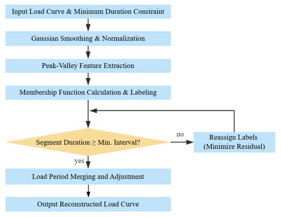
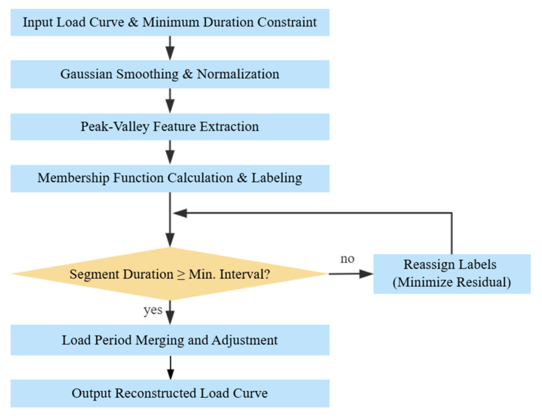
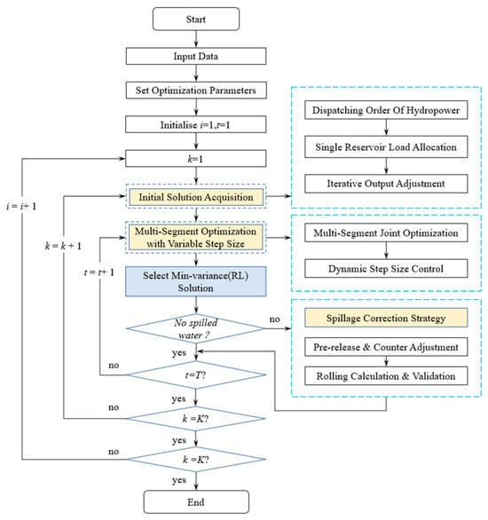
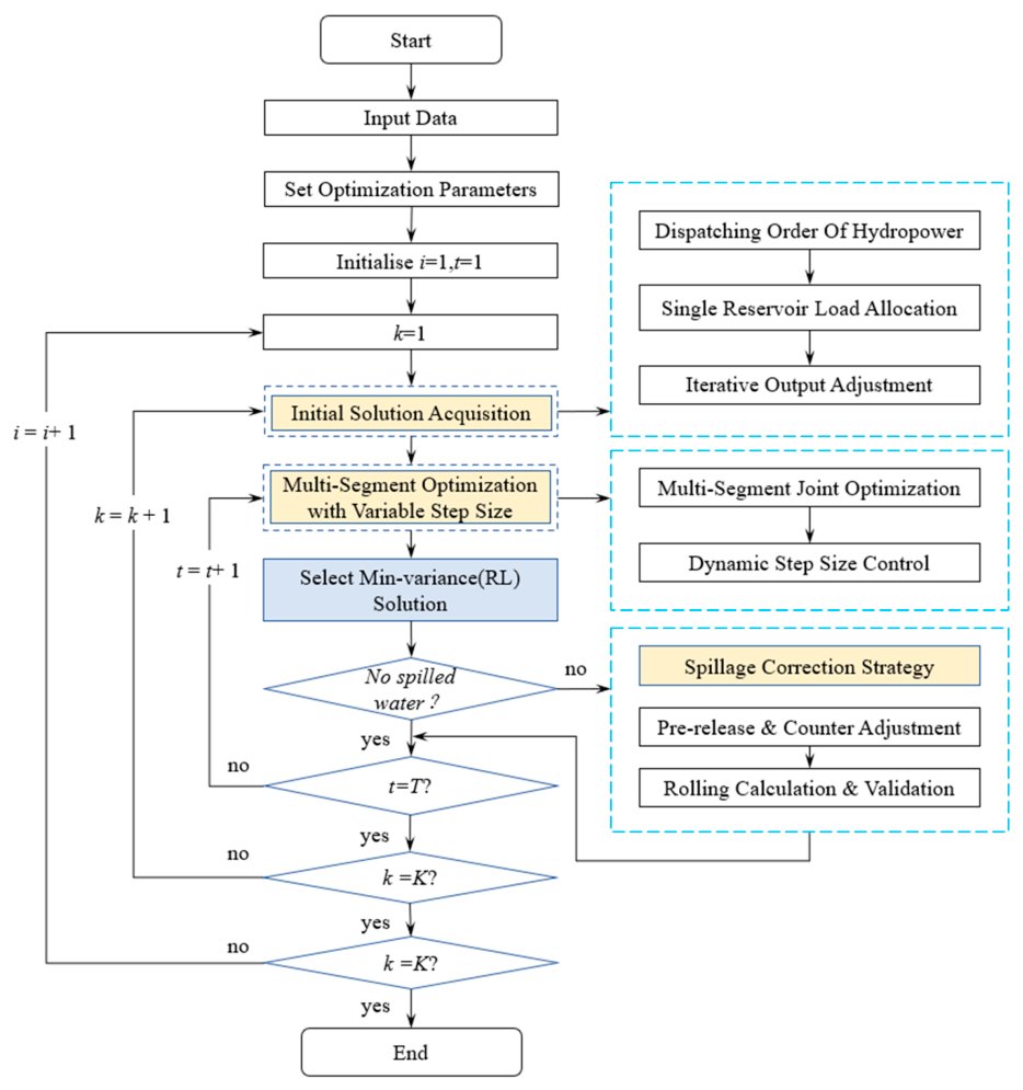
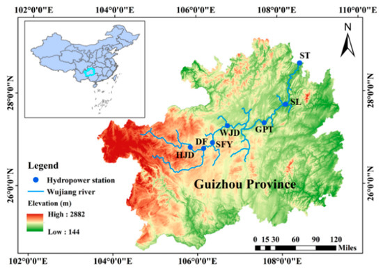
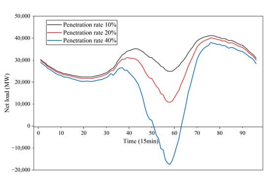
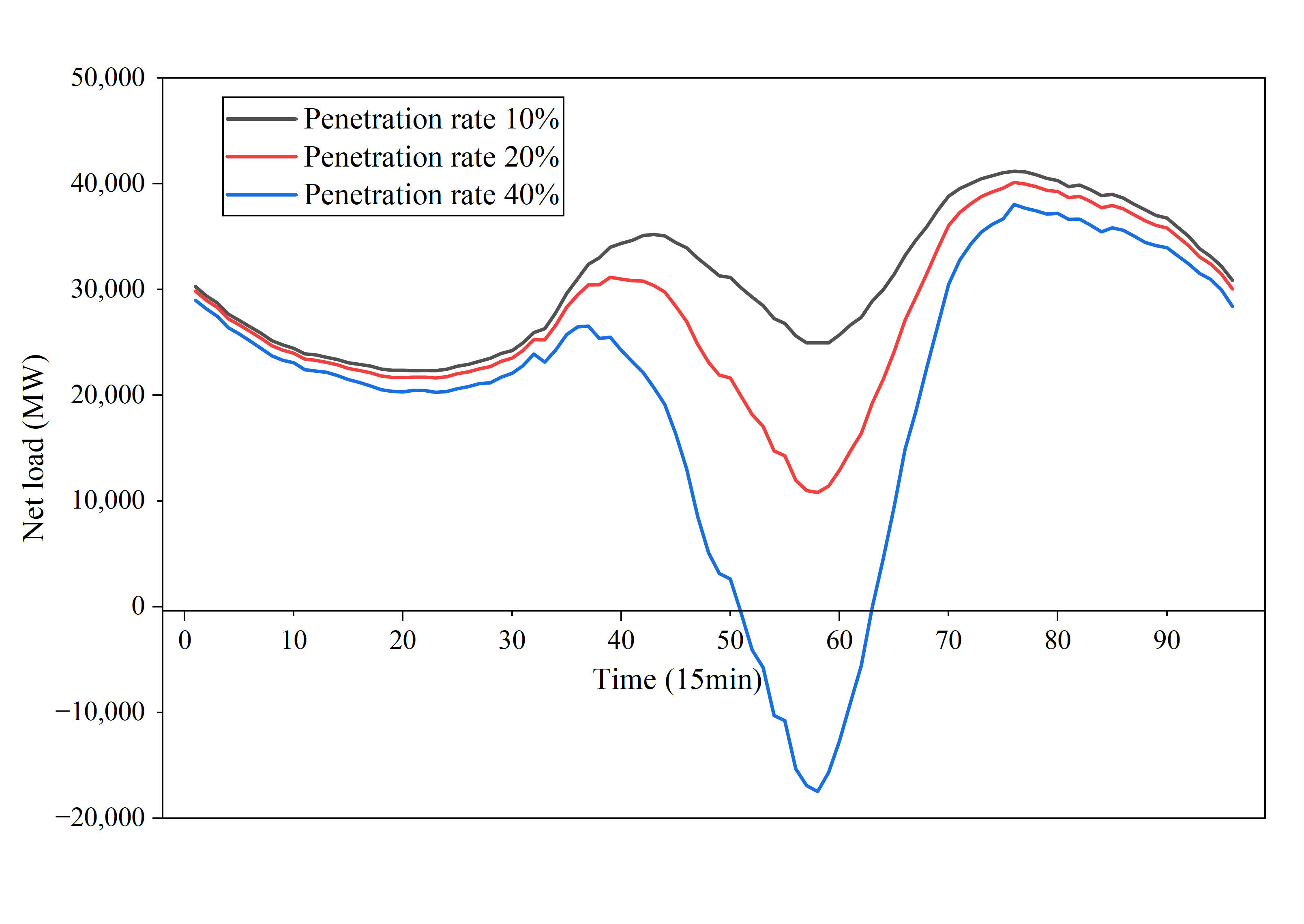
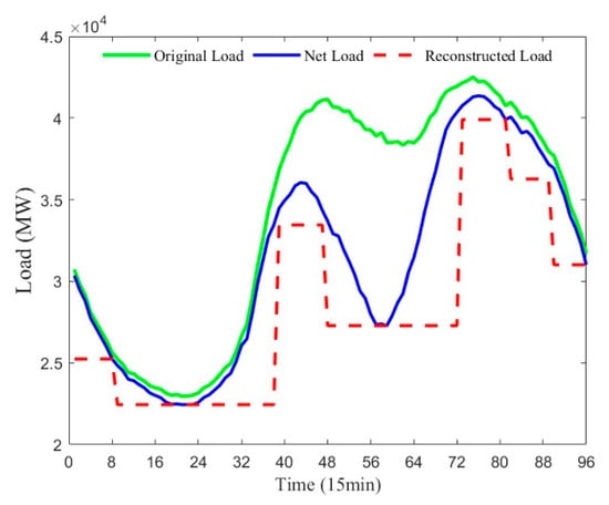
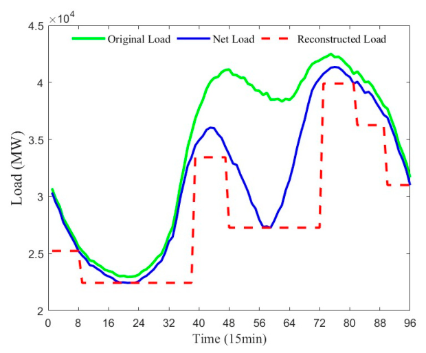
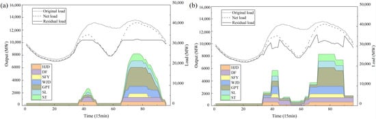
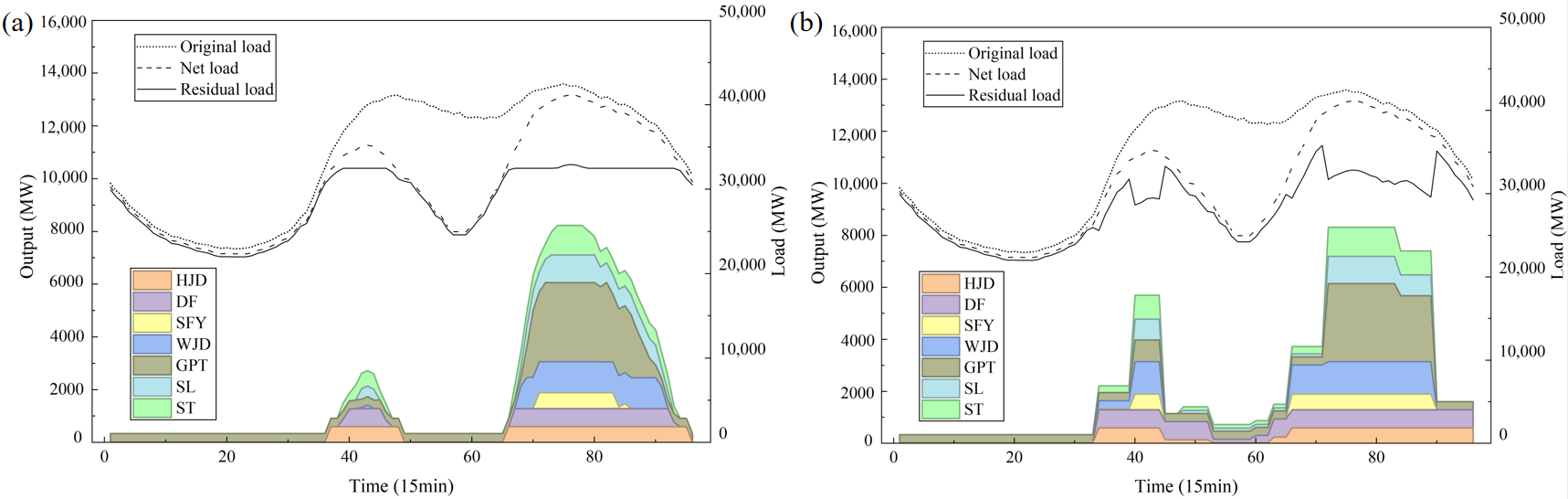
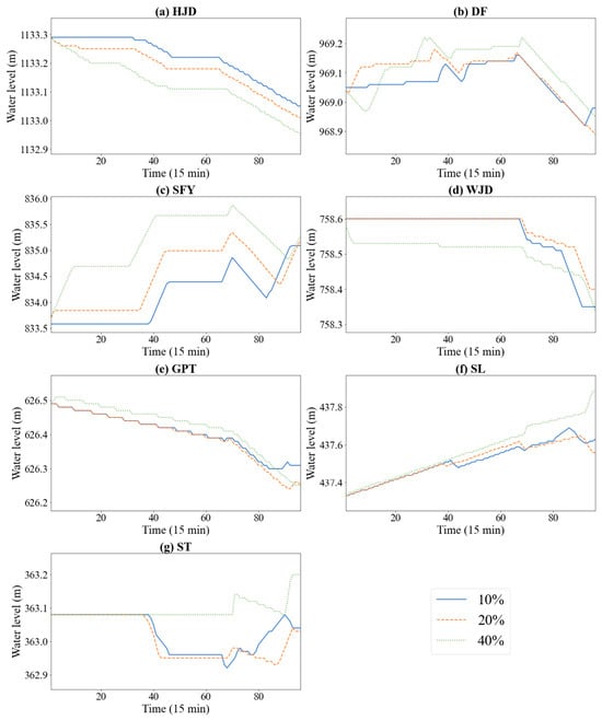
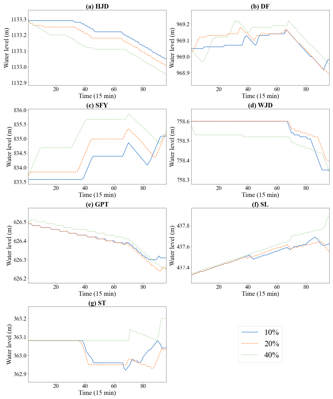
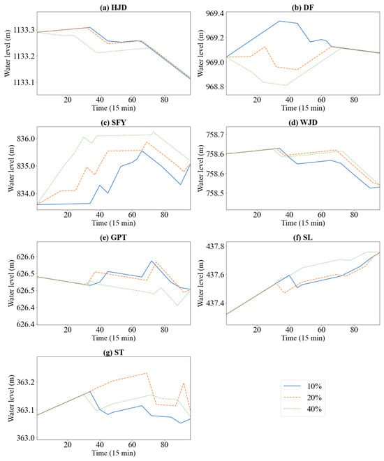
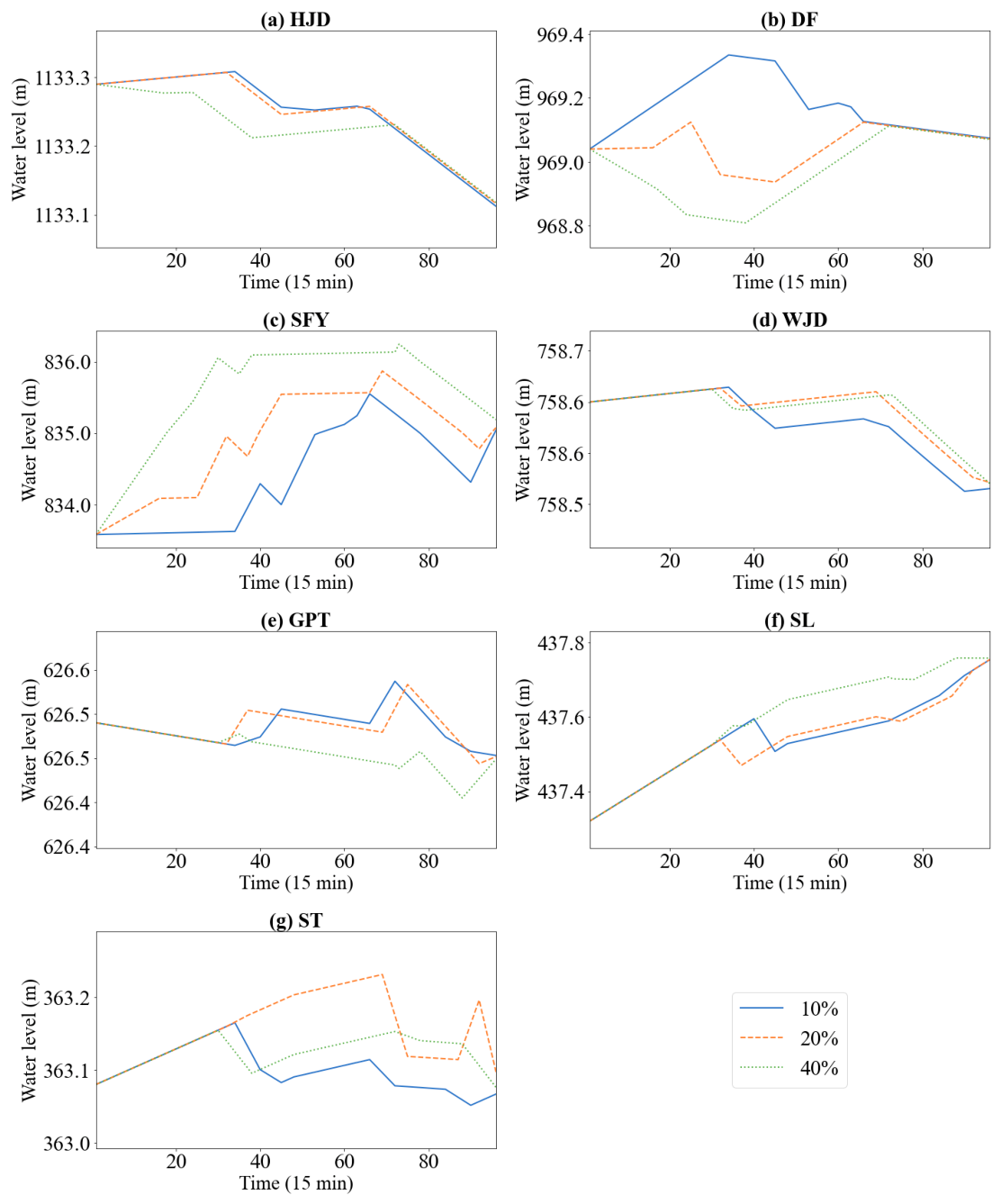

Disclaimer/Publisher’s Note: The statements, opinions and data contained in all publications are solely those of the individual author(s) and contributor(s) and not of MDPI and/or the editor(s). MDPI and/or the editor(s) disclaim responsibility for any injury to people or property resulting from any ideas, methods, instructions or products referred to in the content. |
© 2026 by the authors. Licensee MDPI, Basel, Switzerland. This article is an open access article distributed under the terms and conditions of the Creative Commons Attribution (CC BY) license.