


Abstract
This study provides a practice-oriented sensitivity analysis of DeePC for pressure management in water distribution systems. Two public benchmark systems were used, Fossolo (simpler) and Modena (more complex). Each run fixed a monitored node and pressure reference, applied the same randomized identification phase followed by closed-loop control, and quantified performance by the mean absolute error (MAE) of the node pressure relative to the reference value. To better characterize closed-loop behavior beyond MAE, we additionally report (i) the maximum deviation from the reference over the control window and (ii) a valve actuation effort metric, normalized to enable fair comparison across different numbers of valves and, where relevant, different control update rates. Motivated by the need for practical guidance on how hydraulic boundary conditions and algorithmic choices shape DeePC performance in complex water networks, we examined four factors: (1) placement of an additional internal PRV, supplementing the reservoir-outlet PRVs; (2) the control time step ; (3) a uniform reservoir-head offset ; and (4) DeePC regularization weights . Results show strong location sensitivity, in Fossolo, topologically closer placements tended to lower MAE, with exceptions; the baseline MAE with only the inlet PRV was 3.35 [m], defined as a DeePC run with no additions, no extra valve, and no changes to reservoir head, time step, or regularization weights. Several added-valve locations improved the MAE (i.e., reduced it) below this level, whereas poor choices increased the error up to ~8.5 [m]. In Modena, 54 candidate pipes were tested, the baseline MAE was 2.19 [m], and the best candidate (Pipe 312) achieved 2.02 [m], while pipes adjacent to the monitored node did not outperform the baseline. Decreasing across nine tested values consistently reduced MAE, with an approximately linear trend over the tested range, maximum deviation was unchanged (7.8 [m]) across all cases, and actuation effort decreased with shorter steps after normalization. Changing reservoir head had a pronounced effect: positive offsets improved tracking toward a floor of ≈0.49 [m] around ≈ +30 [m], whereas negative offsets (below the reference) degraded performance. Tuning of regularization weights produced a modest spread (≈0.1 [m]) relative to other factors, and the best tested combination (λy, λg, λu) = (102, 10−3, 10−2) yielded MAE ≈ 2.11 [m], while actuation effort was more sensitive to the regularization choice than MAE/max deviation. We conclude that baseline system calibration, especially reservoir heads, is essential before running DeePC to avoid biased or artificially bounded outcomes, and that for large systems an external optimization (e.g., a genetic-algorithm search) is advisable to identify beneficial PRV locations.
1. Introduction
Urban water distribution systems (WDSs) are complex, mission-critical infrastructures that face significant operational challenges such as high energy use, head losses, and leakage driven by excess pressures [1]. Accordingly, optimal pressure management is a primary means of reducing leakage and improving energy efficiency, typically implemented via pressure-reducing valves (PRVs) placed at strategic locations to regulate pressures at critical demand nodes [1,2,3]. Real-time control (RTC) is required to maintain service levels (pressure/flow/quality) [2,4,5], yet WDS dynamics are nonlinear, high-dimensional, and subject to parametric uncertainty (e.g., pipe roughness, time-varying demand, valve/pump characteristics), which challenges traditional control approaches [1,4].
Model predictive control (MPC) is a common RTC strategy, but it relies on accurate physics-based or state-space models whose development and calibration are costly and difficult on a large scale. Against this backdrop, data-driven approaches have gained traction. Data-Enabled Predictive Control (DeePC) is a method that offers a model-free paradigm that uses measured input–output sequences (historical data) to predict and optimize control actions [4], leveraging the Fundamental Lemma [4,6] and a Hankel matrix representation constructed from the data [7,8,9]. For WDS, DeePC naturally accommodates structural uncertainty and nonlinear behavior [4].
Nevertheless, DeePC performance is sensitive to calibration choices, both algorithmic and system-level. On the algorithmic side, the formulation employs slack variables and regularization weights to balance tracking accuracy against robustness to noise and partial model information, so tuning these regularization weights is therefore critical [4,7,9,10]. On the data/system side, performance depends on the size of the historical data set, the initialization window, and the prediction horizon [4,8]. Moreover, on hydraulic boundary conditions, the placement of an internal PRV is a fundamental design factor that shapes nodal pressures and leakage potential [2,3,5]. The optimal placement of pressure-reducing valves (PRVs) is a fundamental and challenging problem in water-distribution management, typically formulated as a mixed-integer nonlinear programming design problem [1]. The optimization seeks to determine both the locations and the operating settings of the valves so as to maximize their effectiveness in reducing leakage and improving energy efficiency [1,5]. Installing a valve on any branch of the network can dramatically alter the overall hydraulic behavior [1,3], so placement should target points with the highest potential for pressure reduction in downstream subareas [3]. Analyses indicate that employing multiple internal PRVs can achieve more effective pressure management than relying on a single boundary PRV, since distributing valves provides larger pressure margins for leakage control within the monitored areas. Conversely, a suboptimal valve location may leave many critical nodes outside the control region of the existing valves [2], thereby directly impairing the system’s ability to meet the required pressure target and, indirectly, the performance of DeePC. In addition, the reservoir head sets the available energy and governs service levels. In systems experiencing failures (e.g., pipe or pump failures), reservoirs with sufficient stored volume can mitigate or even eliminate supply shortfalls. The effective network pressure directly determines the service level; if the pressure at a node falls below the service-head threshold, the delivered supply may decrease, and if it drops below the minimum-head threshold, supply may cease altogether. Empirically, the head and operational management of reservoirs exert a strong influence on overall network reliability [11]. Accordingly, the performance of DeePC aimed at minimizing the pressure tracking error at a critical node is markedly affected by the system’s overall level of potential energy provided by the reservoirs. In online implementation, a key operational parameter is the control time step , i.e., the frequency at which the optimization is updated. In online implementation, a key operational parameter is the control time step (Δt), i.e., the frequency at which the optimization is updated, as it is a critical factor in DeePC. Similar to MPC, DeePC operates in a receding-horizon manner: solving the optimization yields an optimal input sequence over the prediction horizon , yet only the first action of this sequence is applied immediately to the system. After Δt control steps (with ), the problem is re-solved by updating the most recent measurements , thereby shifting the prediction horizon forward. Choosing reduces the number of times online optimization is required and thus lowers the computational burden. However, the update frequency () must be selected in accordance with the system’s dynamics and feedback delay, if is too large, the controller’s ability to react to changes in real time may be impaired. Therefore, a sensitivity analysis with respect to is essential to determine the optimal balance between computational efficiency and the achieved control quality (MAE) [4,7].
Against this background, the present study aims to provide a comprehensive, practice-oriented sensitivity analysis of DeePC for pressure management in WDS, quantifying how network/system factors (topology/boundary conditions) and algorithmic choices (parameterization/update frequency) affect the mean absolute error (MAE) of the controlled-node pressure relative to a fixed reference. We systematically examine the following: (1) the impact of internal PRV placement on the hydraulic topology and controller benefit [3]; (2) the effect of reservoir head on dynamics and control effort [11]; (3) the effect of the control time step (online optimization frequency) [4]; and (4) the effect of regularization weights on the balance between accuracy and robustness [7,8]. The resulting insights support reliable and efficient deployment of DeePC for complex operational and optimization tasks in water networks.
2. Methodology
DeePC is a model-free control approach that enables real-time optimal decision making for unknown or uncertainty-affected systems, without requiring an explicit mathematical model. Unlike standard MPC, which relies on system identification and calibration of a state space model, DeePC uses raw input–output samples from the system’s history to predict future behavior and derive optimal control actions [4,7].
DeePC builds on Behavioral Systems Theory and the Fundamental Lemma of Willems et al. The Lemma states that, for a linear time-invariant system, the set of all possible trajectories can be spanned by a linear combination of past data, provided the data are persistently exciting [12]. Accordingly, a Hankel matrix is constructed from an offline historical data sequence of length , and partitioned into “past” and “future” blocks:
where supply the initialization information , and are used to predict over the horizon . At each time step , the algorithm solves an optimization problem to determine the decision vector that links the most recent measurements to the future input–output sequence via the Hankel matrices. For water systems exhibiting nonlinearity and measurement noise, the standard formulation is extended to regularized DeePC. The problem minimizes a cost composed of reference-tracking error, control effort, and regularization terms:
subject to dynamic and physical constraints:
In Equations (2) and (3), and denote, respectively, the valve setting inputs (PRV head settings) and the monitored node pressure over the prediction horizon ; are the most recent samples (“past window”) used for initialization; is the behavioral mixing vector selecting a linear combination of past trajectories from the Hankel columns; and are slack variables that relax the past data consistency on the input and output blocks. The regularization weights act exactly where they appear in (2): promotes parsimonious, robust combinations (guards against overfitting to noise); penalizes deviations on the input-consistency block (e.g., actuation/excitation imperfections); and penalizes deviations on the output consistency block (measurement noise/model mismatch).
Offline, we collect a persistently exciting data record of length and assemble the Hankel blocks . Before online operation, we select the hyperparameters (initialization window) and (prediction horizon), the control time step , and the regularization weights . Online, at each control instant, we measure/update , solve (2) and (3) subject to bounds, and apply only the first input from the optimized sequence ; after , the horizon is shifted (receding-horizon operation), measurements are refreshed, and the problem is re-solved [4,7].
The water-distribution systems used in the studies by Fossolo and Modena were obtained from the Water Benchmark Hub [13,14]. We first validated our control implementation by running DeePC on the Fossolo network under the same conditions reported by Perelman and Ostfeld [4], expecting to reproduce their MAE values to a close approximation. All optimization problems in DeePC were solved with the Gurobi Optimizer (default settings). Hydraulic simulations were carried out in EPANET via EPyT (Python 3.11) [15], and the DeePC framework was implemented using the public PyDeePC library following Coulson’s research [7], which is also the code base used by Perlman and Ostfeld [4]. After reproducing comparable results, we proceeded to develop and execute the sensitivity analyses.
Each run followed a two-stage DeePC routine, randomized data collection followed by closed-loop control. In all figures, the grey segment marks identification and the white segment marks control, both in the pressure plot and in the PRV setting plot. For each sensitivity setting, we re-collected a fresh identification dataset using the same randomized excitation with a fixed seed, and rebuilt the Hankel matrices; no identification data were reused across settings. Thus, DeePC was re-initialized under the conditions tested rather than transferred from a different operating point. The control input is the PRV opening (head setting), and the measured output is the pressure at the monitored node. Hankel matrices were assembled from the last samples of the identification phase. We note that alternative Hankel constructions exist in the literature, but we kept this choice fixed across scenarios to ensure fair comparisons. We used the same randomized excitation with a fixed seed in every setting, and identification data were re-collected per setting, which reduces scenario variance while introducing a mild seed dependence (observed as small MAE deviations across seeds, without altering conclusions). Unless otherwise specified by a sensitivity test, the baseline settings were as follows: time step = 1 [h], identification window = 48 [h], prediction horizon = 12 [h], closed-loop control phase duration = 1 week, and the data-collection phase comprised 600 steps. The performance metric is MAE [m] of the monitored node pressure relative to its reference value, computed over the control window only.
In the Modena case study, in addition to MAE, we report two complementary performance indicators computed over the closed-loop control window only. Let index the control samples, let denote the monitored node pressure, and let denote the fixed pressure reference. Define the tracking error . The MAE is
To capture worst-case tracking, we also compute the maximum absolute deviation from the reference:
To quantify valve actuation effort, consider active PRVs in a given run (including both fixed and added valves, as applicable), and let denote the valve setting command of PRV at control sample . We define the cumulative actuation effort as the sum of absolute inter-sample changes across all valves:
For all sensitivity analyses except the test, actuation effort is reported normalized by the number of valves to enable fair comparison across scenarios with different numbers of PRVs. In the sensitivity analysis, where the number of control updates changes with the sampling rate, the valve actuation effort is additionally normalized by the number of control phase steps (equivalently, by the control duration in hours) to obtain a per-step/per-hour average actuation per valve. This prevents the summed effort from artificially increasing as decreases simply because more actuation increments are accumulated.
In the reservoir head sensitivity test, intentionally perturbs the hydraulic boundary conditions; therefore, for sufficiently negative , the 28 [m] reference at the monitored node may become hydraulically unattainable. In such cases, MAE is still reported as a consistent reference tracking metric, and the outcome is interpreted as a service-feasibility limitation rather than a controller tuning limitation. To allow for replication, Table A1 in Appendix A summarizes the baseline parameters that were kept constant throughout the run unless explicitly changed by a sensitivity test.
For pressure regulation from the sources, PRVs were added near the reservoirs in both networks, and baseline reservoir heads were explicitly modified relative to the Benchmark networks: Fossolo +14 [m] at the reservoir and in Modena +25 [m] applied to all reservoirs. In Fossolo, the reservoir adjacent valve acts as the fixed PRV (Valve 59), while Valve 58 is the tested PRV; it is substituted in place of each candidate pipe during the code run and evaluated as the additional PRV. In Modena, we did not attempt an exhaustive scan. Instead, we assembled a random informed subset of 54 candidate pipes as follows: (i) start from a uniform random sample; (ii) retain pipes that, in the baseline steady state snapshot, exhibited relatively high throughputs, non-negligible headloss, or a topologically strategic role (e.g., main trunks or inter-zone connectors); and (iii) force include the two pipes adjacent to the monitored node (274, 275) to enable a near-node comparison. Baseline EPANET flows/headlosses were used only for pre-screening and were not fed to the controller. The resulting set is representative but non-exhaustive; consequently, the reported “best” location is the best among those tested.
From the outset, all PRV installations were constrained to preserve the network’s original flow directions. To enforce this, at each iteration after positioning the PRV and executing the DeePC run, we inspected the flow sign along the tested pipe over the entire run. If the flow remained zero or negative and did not change sign during that run, we reversed the valve orientation and re-ran the case, thereby restoring a positive, physically admissible flow consistent with the original direction. Installing a PRV against the prevailing flow effectively blocks the pipe and may impair the operation of the DeePC controller. In Fossolo, no sign changes occurred during runs; in Modena, some pipes did show sign changes within a run, and at this stage of the study, such pipes were excluded from analysis and conclusions.
Beyond analyzing additional valve placements, three sensitivity studies were performed, holding all other settings fixed under the same control protocol: (1) control time step—runs at several steps while keeping the number of identification steps identical and the total control duration identical; (2) reservoir head offsets—in Modena, a uniform was applied to all reservoirs relative to baseline, and DeePC was re-run under otherwise identical conditions; and (3) regularization weights (“lambdas”) (measurement slack), (penalty on the mixing vector), and (actuation change smoothing). The search ranges for the lambdas followed Coulson’s guidance [7] and were scanned on a logarithmic grid, at each stage one weight was varied while the other two were held constant, and the roles were then cycled. Given this coarse “one factor at a time” sweep (three logarithmically spaced levels per weight), the analysis provides a local indication only and does not warrant inference about global linear or non-linear trends.
3. Case Studies
To assess how various factors influence DeePC performance, we conducted sensitivity analyses on two water distribution systems: Fossolo (simpler) and Modena (more complex). The network models were taken intact from a public repository [13,14]. The only modifications to the original files were (1) adding pressure-reducing valves (PRVs) near each reservoir which function as the control actuators that regulate the system pressure, and (2) increasing the source head to allow sufficient excess head to maintain the desired pressure levels of the system: +14 [m] in Fossolo and +25 [m] for every reservoir in Modena. No other changes were made to the models. Within this setup, several factors were examined for their effect on method performance.
3.1. Fossolo Case Study
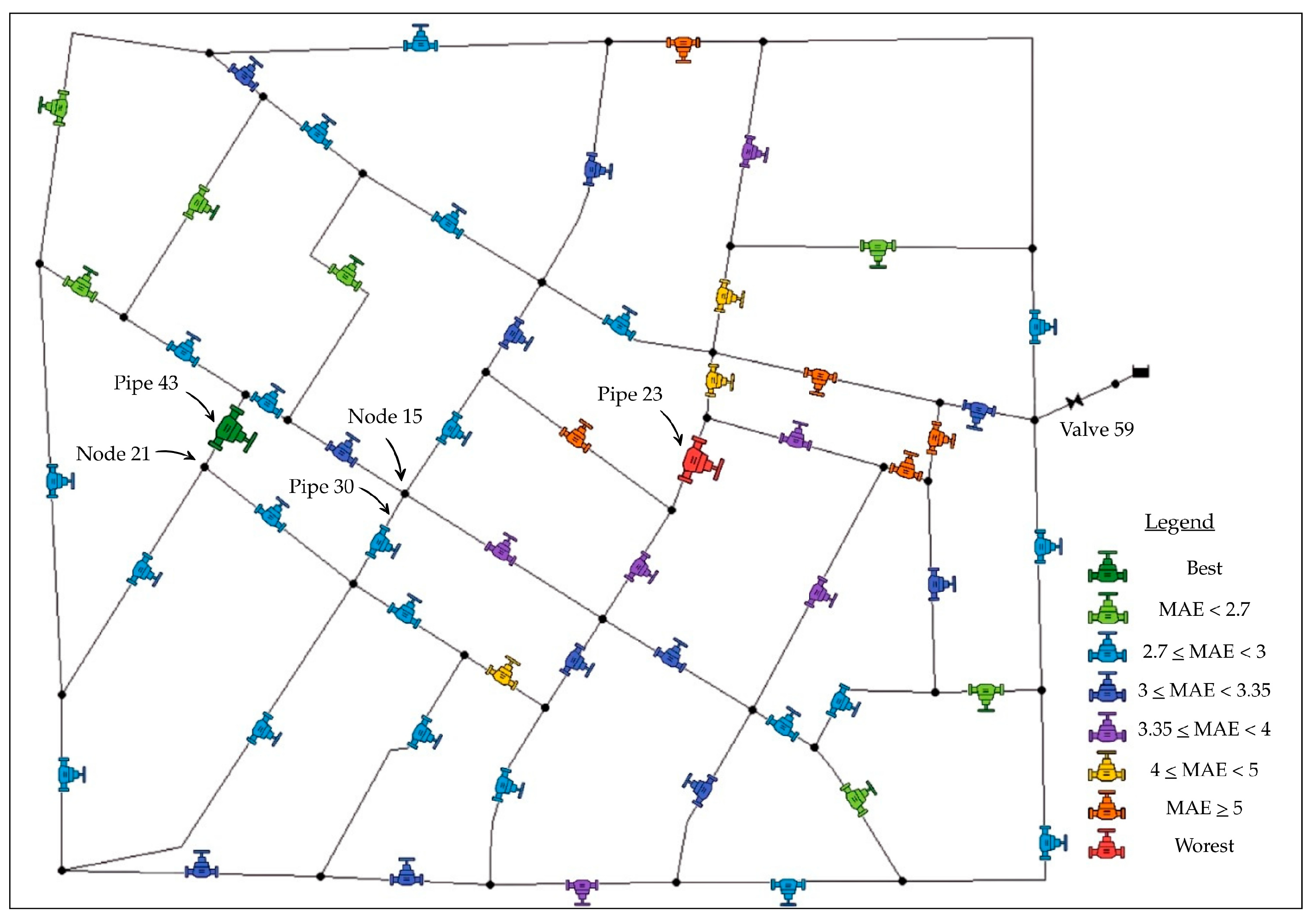
As part of the sensitivity analysis, the Fossolo network served as the first case study, as shown in Figure 1. Node 21 was selected as the monitored node, with a pressure reference of 30 [m]. In Fossolo, we evaluated the effect of adding one additional PRV within the network. Each pipe was tested as a secondary valve candidate in turn. The pipe was temporarily replaced by a PRV, a DeePC experiment was run, and the MAE of the pressure at Node 21 relative to 30 [m] was computed. The pipe was then restored before proceeding to the next. All runs comprised the same randomized identification phase, followed by closed-loop control using DeePC.
Figure 1.
Fossolo network with labels for the pipes, nodes, the reservoir, and the relevant valve. A spatial visualization of the search results for the location of an additional pressure-reducing valve (PRV). Each pipe is marked with a PRV icon color-coded by the MAE bin (see legend). The best candidate is highlighted by a larger green icon and the worst by a larger red icon. In all runs, PRV 59 was kept fixed while PRV 58 was moved across pipes; MAE is computed for the pressure at Node 21 relative to the 30 [m] reference.
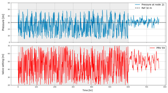
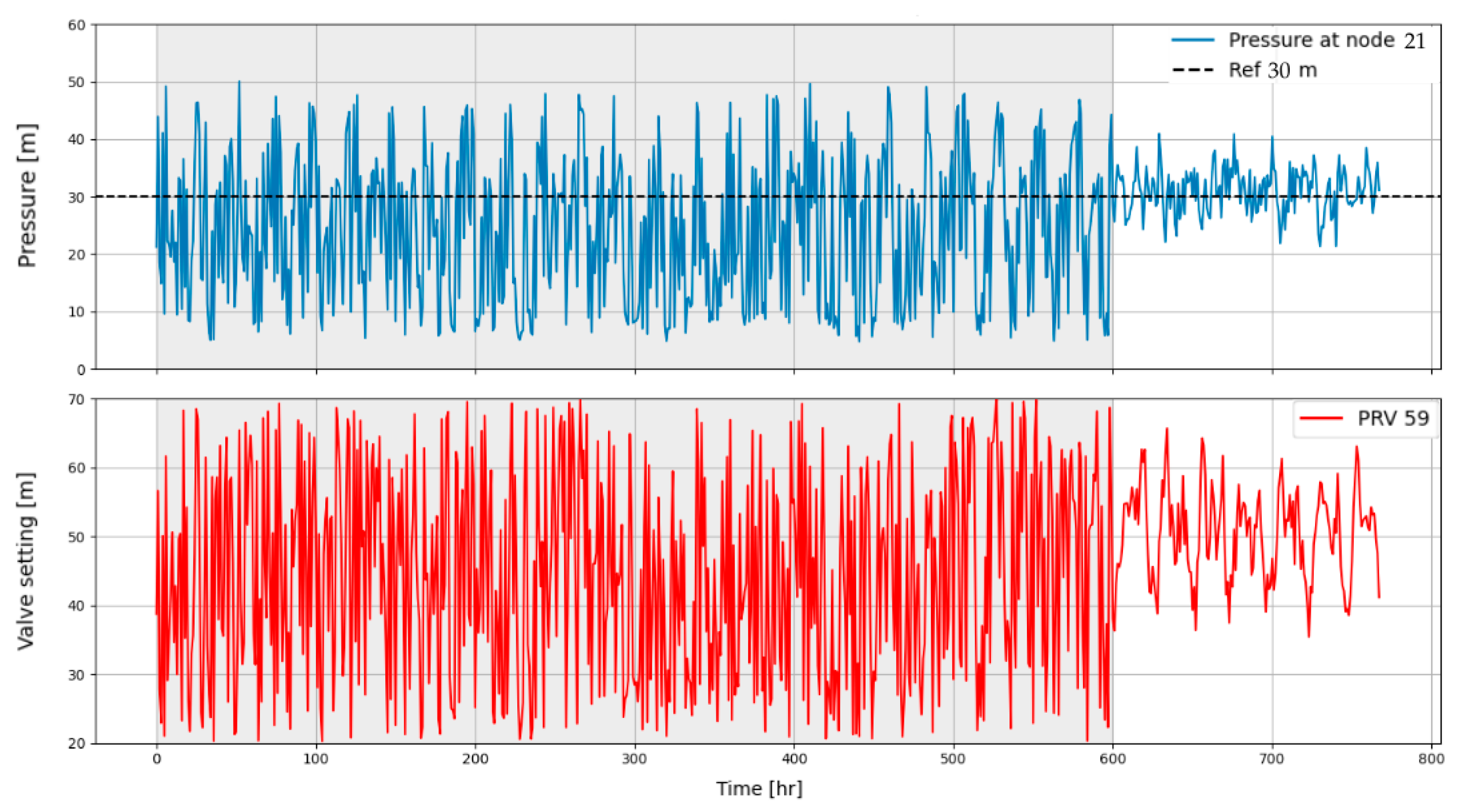
As a reference baseline (see Figure 2), we ran DeePC on the Fossolo network with PRV 59 as the only actively controlled valve, with no additional changes or interventions. The experiment settings match those used in the comparison runs. During the control phase, the pressure at Node 21 tracked the 30 [m] reference with a mean absolute error (MAE) of 3.35 [m]. This value serves as the baseline for comparison, and subsequent experiments are compared against this MAE to determine whether each intervention improves or degrades performance and by how much.
Figure 2.
Baseline configuration with no additional pressure-reducing valve (PRV), used for performance comparison: The top plot shows the pressure at Node 21, where the pressure sensor is located, over time. The dashed line marks the 30 [m] reference of desired pressure. The bottom plot shows the pressure setting of the PRV at the system inlet. The grey segment marks the randomized data-collection/identification phase, and the white segment marks the closed-loop control phase using DeePC. The run is performed under the same experiment conditions as the location-search experiments and serves as the baseline for computing the MAE.
As shown in Figure 1, the additional PRV location yields a wide range of outcomes; some locations improve the MAE relative to the baseline (3.35 [m]), while others degrade it. The legend splits results into values below 3.35 [m] and above 3.35 [m]. The best location is Pipe 43, whereas the worst is Pipe 23. A pattern emerges whereby locations closer to Node 21 in network path length tend to improve the MAE, with some more distant locations also providing improvements.
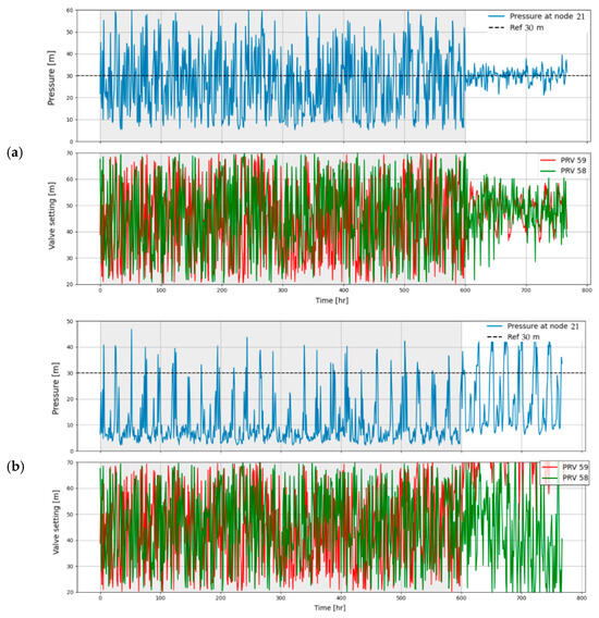
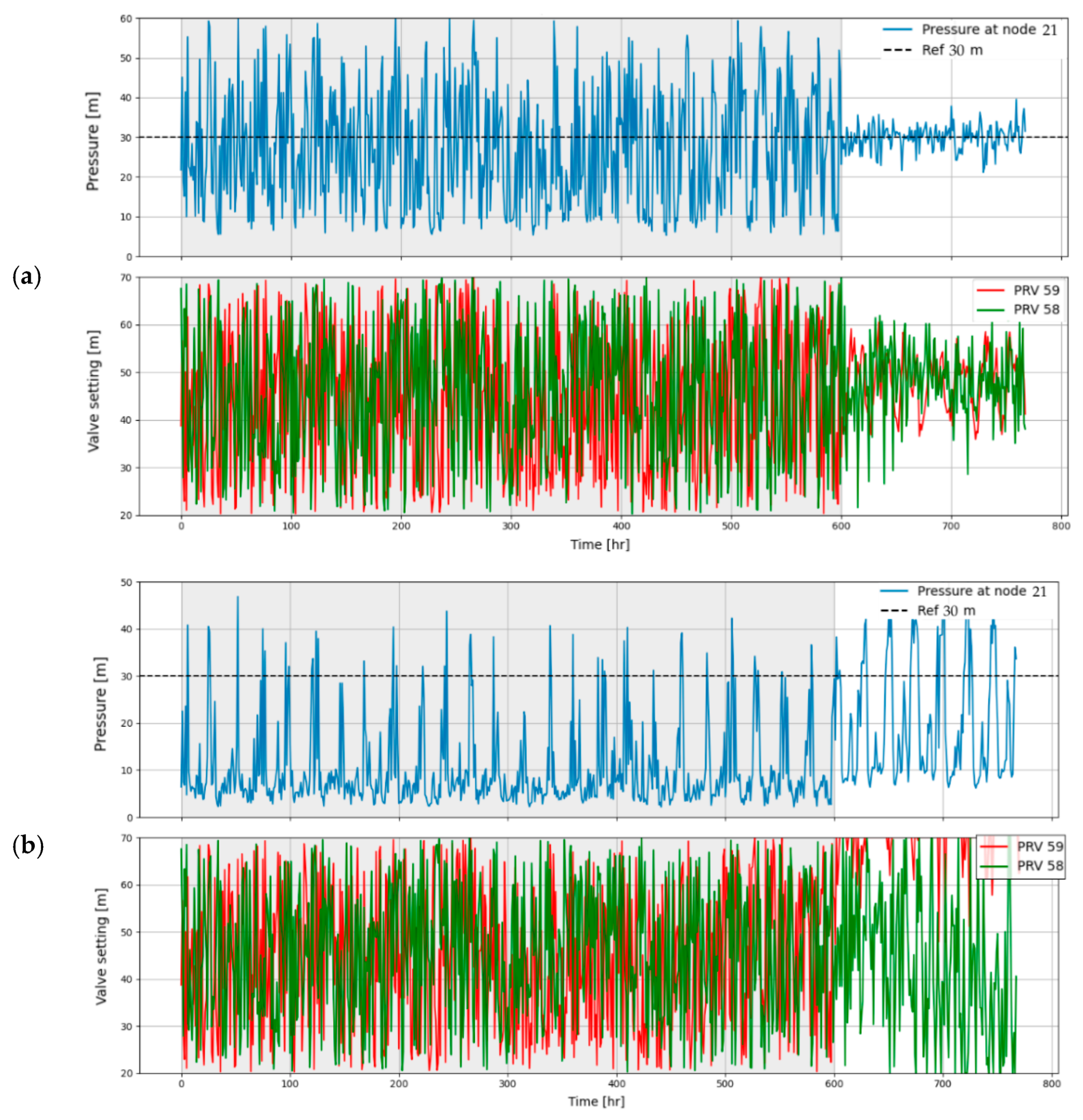
In Figure 3, we compare two locations for the additional valve: (a) Pipe 43 (best) and (b) Pipe 23 (worst). In Figure 3a, once the closed-loop control begins (white background), the pressure at Node 21 settles near the 30 [m] reference with reduced variance. The valve-setting plot shows balanced participation of the two valves, and their settings vary across the range without lingering at extremely high or low values. In Figure 3b, the pressure stays low for extended periods and does not cleanly converge. The valve-setting plot shows PRV 58 carrying most of the control effort, whereas PRV 59 (near the reservoir) remains near its upper limit for long intervals, almost fully open, so its contribution to controlling the node pressure is negligible.
Figure 3.
Impact of the additional PRV location on the control performance. In each panel: The top plot shows the pressure at the monitored node over time (dashed line= 30 [m] reference), and the bottom plot shows the PRV pressure settings, PRV 59 is the fixed (baseline) valve, and PRV 58 is the additional valve whose location is varied across pipes. The grey segment indicates the randomized data-collection/identification phase, and the white segment indicates the closed-loop control phase using data-enabled predictive control (DeePC). (a) Best location, selected by minimizing the MAE of the controlled-node pressure relative to the reference; (b) worst location under the same experiment setup and plotting conventions.
To assess generality, we repeated the location-search experiment for another monitored node, Node 15, under identical settings. Results followed the same pattern observed in the Node 21 monitoring case: locations closer in network path length (number of links) to the monitored node tended to yield lower MAE, with occasional exceptions. For example, the best location for Node 15 was Pipe 30, adjacent to Node 15, mirroring the result obtained when Node 21 was the monitored node.
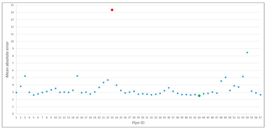
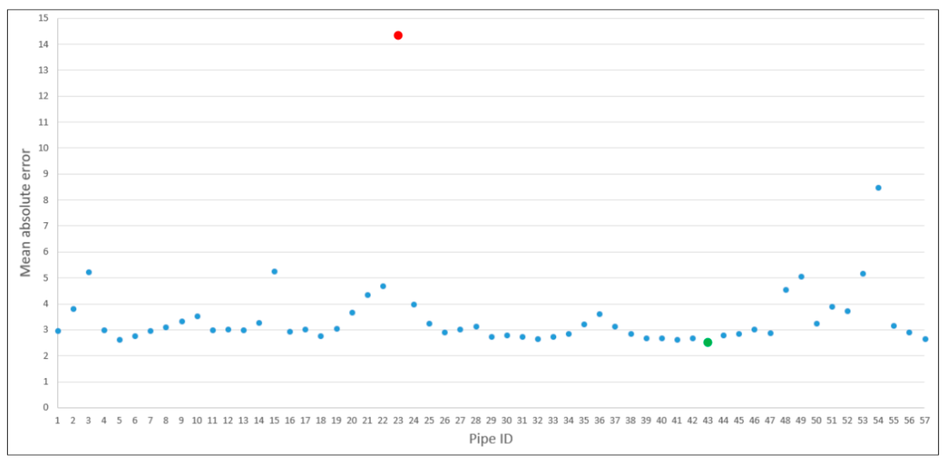
To consolidate the search outcomes in the first experiment (when Node 21 was monitored), Figure 4 plots the MAE for every pipe considered as the location of the additional valve. Beyond Pipe 23, the worst outlier (red), several other underperforming candidates are visible, e.g., Pipe 54 with MAE around 8.5 [m], and several additional pipes with MAE in the 4–5.5 [m] range. Conversely, near the best location (green), there are several near ties with comparably low MAE, representing clear improvements over the baseline without an additional PRV. This compact view enables a clear ranking of all candidates and highlights the strong location sensitivity: several placements are “good enough,” whereas a poor choice can markedly degrade performance.
Figure 4.
MAE for each candidate pipe where the additional pressure-reducing valve (PRV) is placed. X-axis: pipe ID, Y-axis: MAE of the pressure at Node 21 relative to the 30 m reference. In all runs, PRV 59 is kept fixed, whereas PRV 58 is installed in turn on each pipe as the candidate. The green dot marks the best location (lowest MAE), and the red dot marks the worst (highest MAE). All experiments were performed under the same identification and control settings.
To assess the influence of dominant flow paths on the error, we ran a simple correlation check. For each candidate location (each pipe), we took two local indicators on the pipe where the PRV was installed: (i) the head loss across the pipe and (ii) the flow through it, and paired each with the MAE obtained for that DeePC run. Scatter plots of MAE vs. Δh and MAE vs. flow (Q) showed no clear or monotonic dependence.
3.2. Modena Case Study
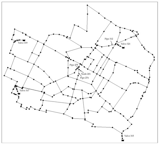
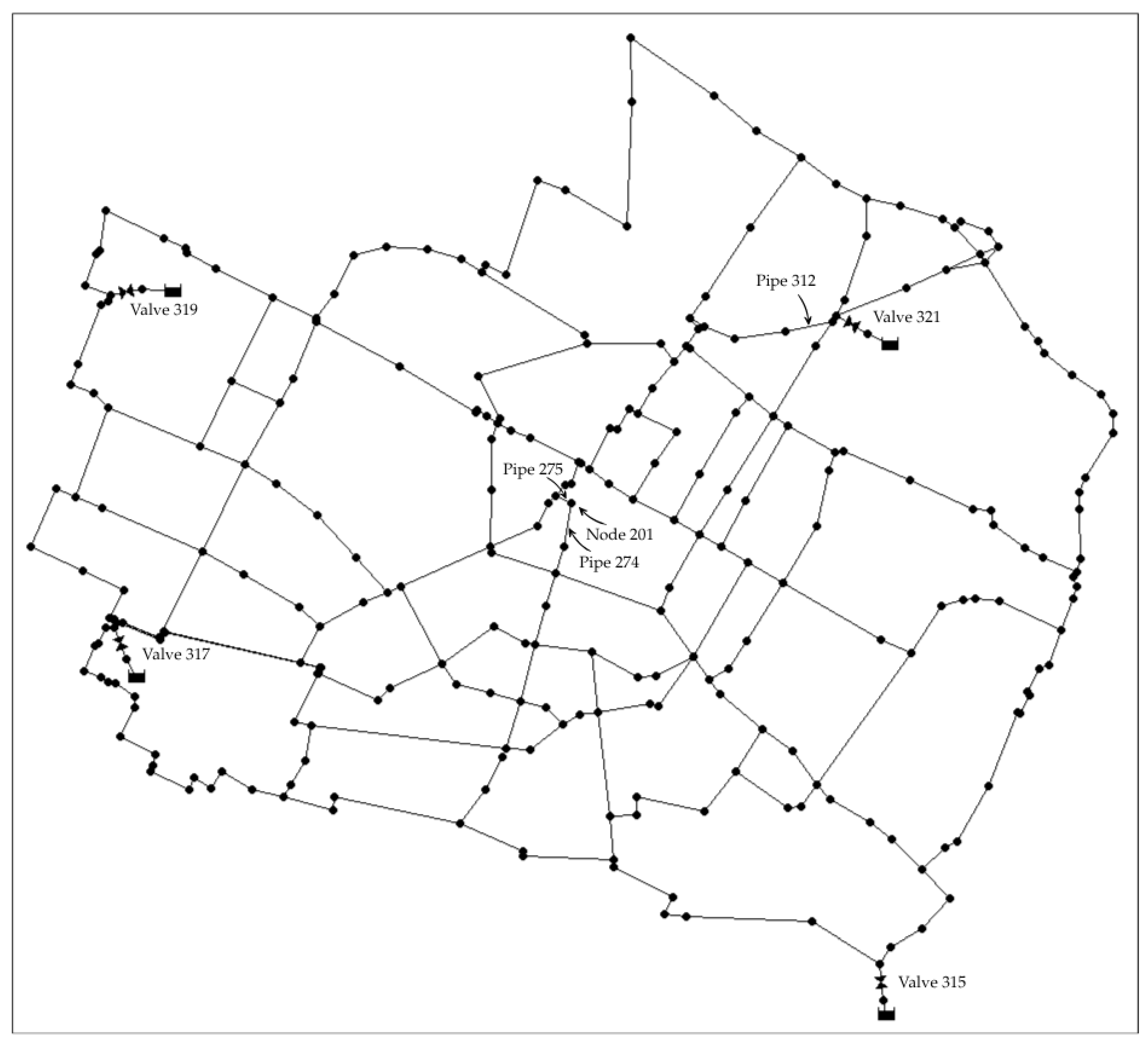
Continuing the sensitivity analysis, the Modena network served as the second case study (Figure 5). It is a larger system supplied by four sources. Node 201 was selected as the monitored node, and the pressure reference was set to 28 [m]. In this section, we examined the effect of several factors on the DeePC performance, including the placement of an additional PRV within the network, while keeping identical experiment settings across all runs (same randomized identification phase followed by closed-loop control). Prior to all sensitivity studies, we executed a baseline DeePC run with no additional modifications, which yielded an MAE of 2.19 [m], a maximum deviation of 7.8 [m], and a valve actuation effort of 1173.09 [m] at Node 201. This baseline was used as the reference for all comparisons and sensitivity cases that reduce the MAE, which is the primary measure in this study, below 2.19 [m] are considered improvements, whereas cases that increase it are considered degradations.
Figure 5.
The Modena water distribution network used in this study, with labels for the components referenced in the paper (valves, selected nodes, and pipes).
3.2.1. Additional Valve
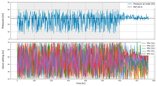
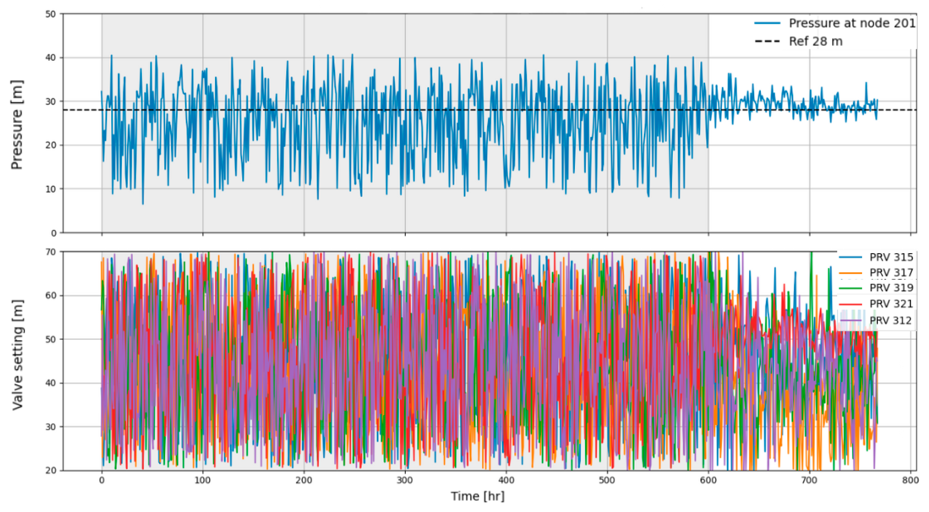
Figure 6 shows the closed-loop DeePC response when the additional valve is placed on Pipe 312. Because the Modena network is large, we evaluated a sample of 54 candidate pipes under identical settings (see the full results in Appendix B). In each run, an additional valve was installed on a candidate pipe, the DeePC experiment was executed, and the MAE of the pressure at Node 201 relative to 28 [m] was computed. Among all candidates, Pipe 312 achieved the lowest MAE but higher maximum deviation and valve actuation effort than the baseline, as can be seen in Table 1. In contrast to the Fossolo case study, pipes near the monitored node (e.g., 274 and 275) did not outperform Pipe 312 in the MAE calculation.
Figure 6.
Experiment assessing whether adding an additional pressure-reducing valve (PRV) improves the MAE. The top plot shows the pressure at Node 201 over time (dashed line = 28 [m] reference), the grey segment denotes the randomized data-collection/identification phase, and the white segment the closed-loop control phase using DeePC. The bottom plot shows the valves’ settings [m] for the active PRVs (PRV 315, 317, 319, 321, and PRV 312—the added valve in this run). Experiment conditions match those of the comparison runs, and the result is used to quantify the effect of the additional valve on the MAE.
Table 1.
Comparison of closed-loop control performance between the baseline configuration and the configuration with an additional internal PRV. Reported metrics are the mean absolute error and maximum deviation of the monitored node pressure from its reference [m], and the valve actuation effort [m] computed over the control phase.
Figure 6 also shows that all valves contribute to control; in particular, PRV 312 provides substantial, sustained actuation. Its settings remain away from the extremes, indicating effective regulation and a direct influence on the pressure at the monitored node, consistent with the behavior of the reservoir-inlet PRVs.
3.2.2. Time Step in DeePC
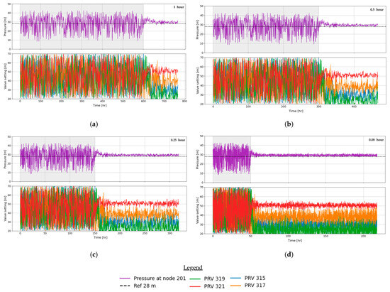
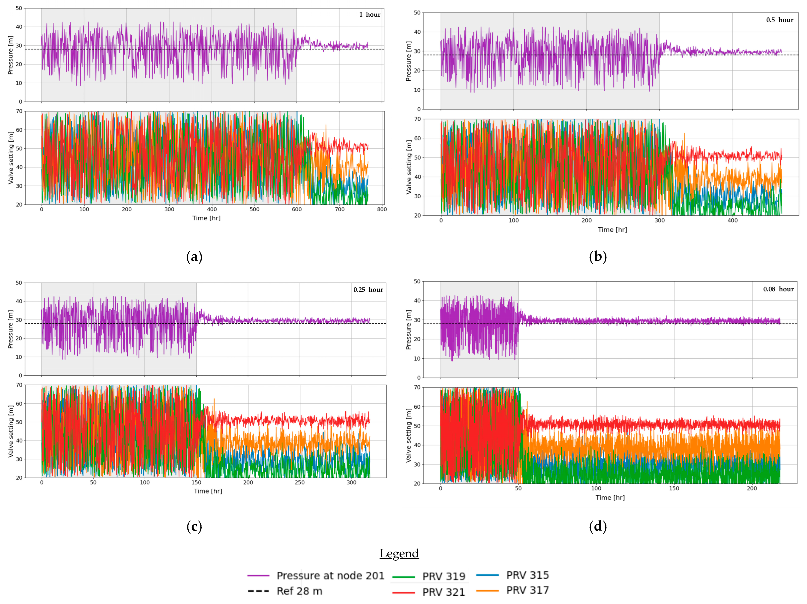
Figure 7 presents a sensitivity analysis of the control time step in DeePC. All runs used the same number of identification samples and the same closed-loop evaluation horizon. Therefore, a smaller time step produces more control updates and a shorter grey identification segment. Figure 7a is the baseline case (time step of 1 h) against which all sensitivities are compared. Qualitatively, in all cases, the pressure at Node 201 settles during the control phase around the 28 [m] reference. The number of control updates required for settling is similar across cases, but when the time step is smaller (e.g., 0.25 h, 0.08 h), the control phase contains many more steps, so the relative portion occupied by settling is smaller. With a larger time step, the same number of steps occupies a larger time fraction and appears longer on the axis. After settling, the oscillations have a relatively small amplitude and no sharp spikes.
Figure 7.
Sensitivity of the control time step in DeePC (sampling interval for updating the PRV settings). In each panel, the top plot shows the pressure at Node 201 over time (dashed line = 28 [m] reference), and the bottom plot shows the valve settings [m]. The grey segment marks the randomized data-collection/identification phase, and the white segment marks the closed-loop control phase. All runs are identical except for the control time step. (a) 1 h; (b) 0.5 h; (c) 0.25 h; (d) 0.08 h. The legend below the panels maps colors to the active valves and indicates the pressure reference line.
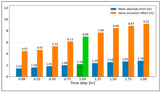
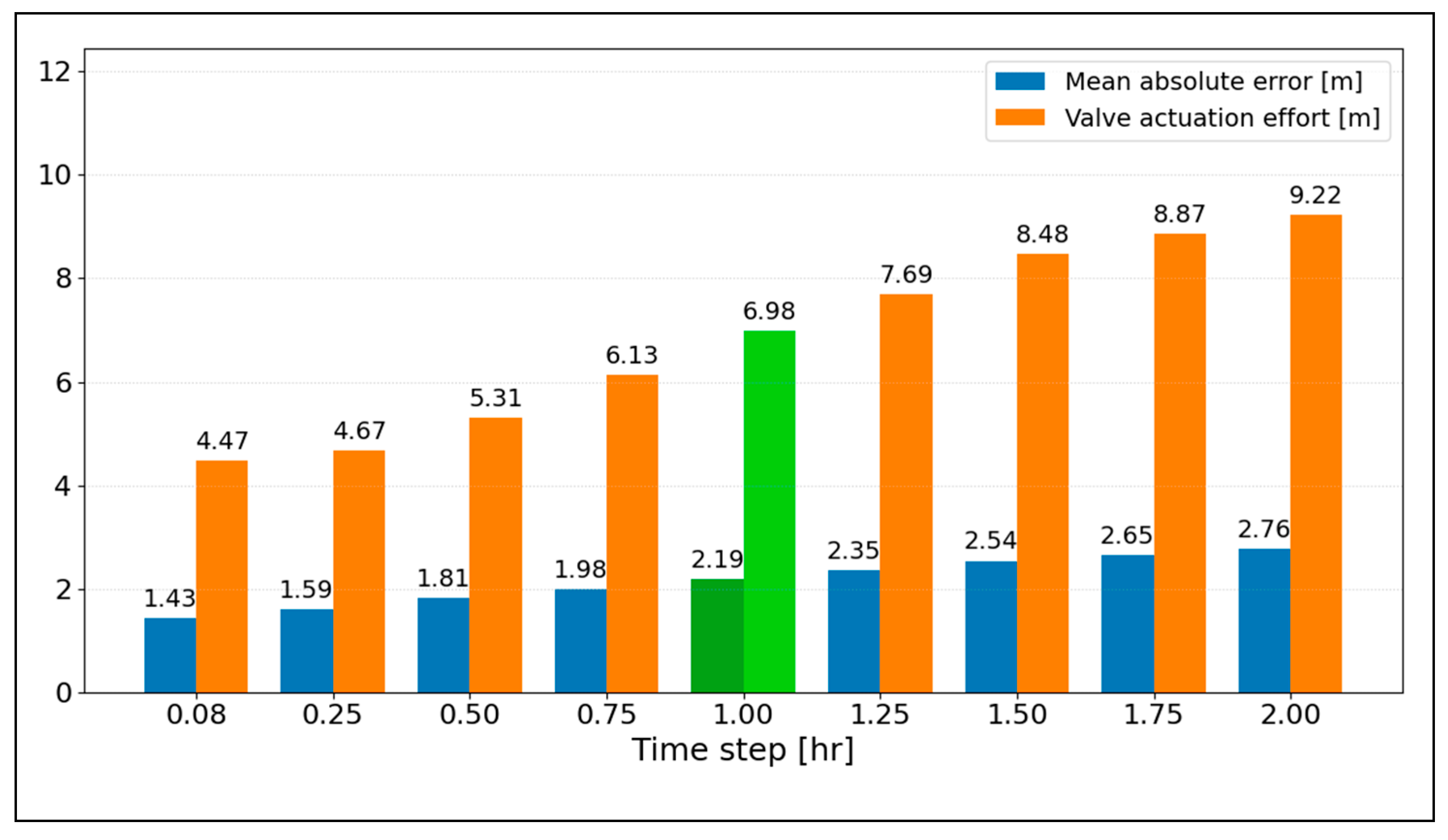
Figure 8 summarizes the sensitivity to the control time step. We tested nine time steps, mostly in 0.25 h increments, plus a short 0.08 h (5 min) case, with the baseline of 1 h highlighted in green. A clear, consistent decrease in MAE is observed as the time step decreases, indicating improved reference tracking under more frequent re-optimization. Consistent with this improvement, the valve actuation effort also decreases as the time step decreases, suggesting smoother control actions at higher update rates (as quantified by the normalized effort definition described in the methodology). In addition, the maximum deviation metric remained unchanged across all tested time steps, yielding the same value of 7.8 [m] for every . Over the tested range, the trend appears approximately linear qualitatively.
Figure 8.
Bar chart summarizing the control time-step sensitivity in DeePC. For each tested control time step (x-axis: time step [h]), bars report (i) the mean absolute error of the controlled-node pressure relative to the 28 [m] reference and (ii) the valve actuation effort over the control phase (both in [m]; y-axis). The baseline time step (1.00 [h]) is highlighted in green: dark green denotes the MAE bar and light green denotes the actuation-effort bar. The remaining MAE bars are shown in blue, and the actuation-effort bars are shown in orange. Values are annotated above the bars. Lower values indicate better performance.
3.2.3. Reservoir Head Change
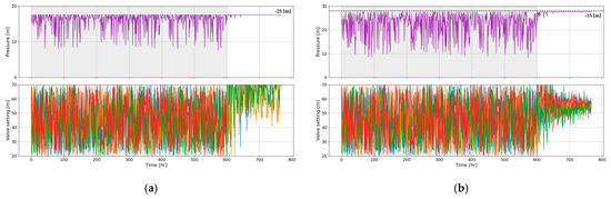
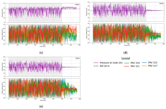
As shown in Figure 9, applying a uniform reservoir-head change strongly affects the closed-loop behavior at Node 201 (baseline for comparison: Figure 7a, ).
Figure 9.
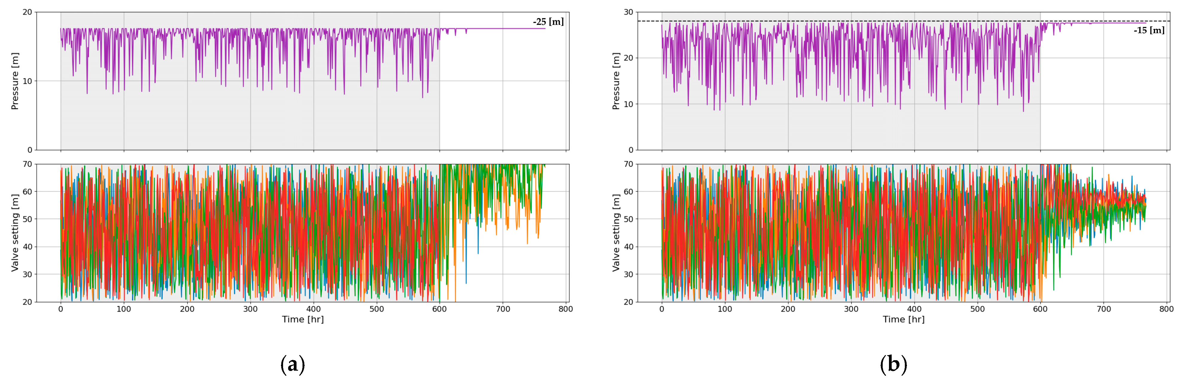
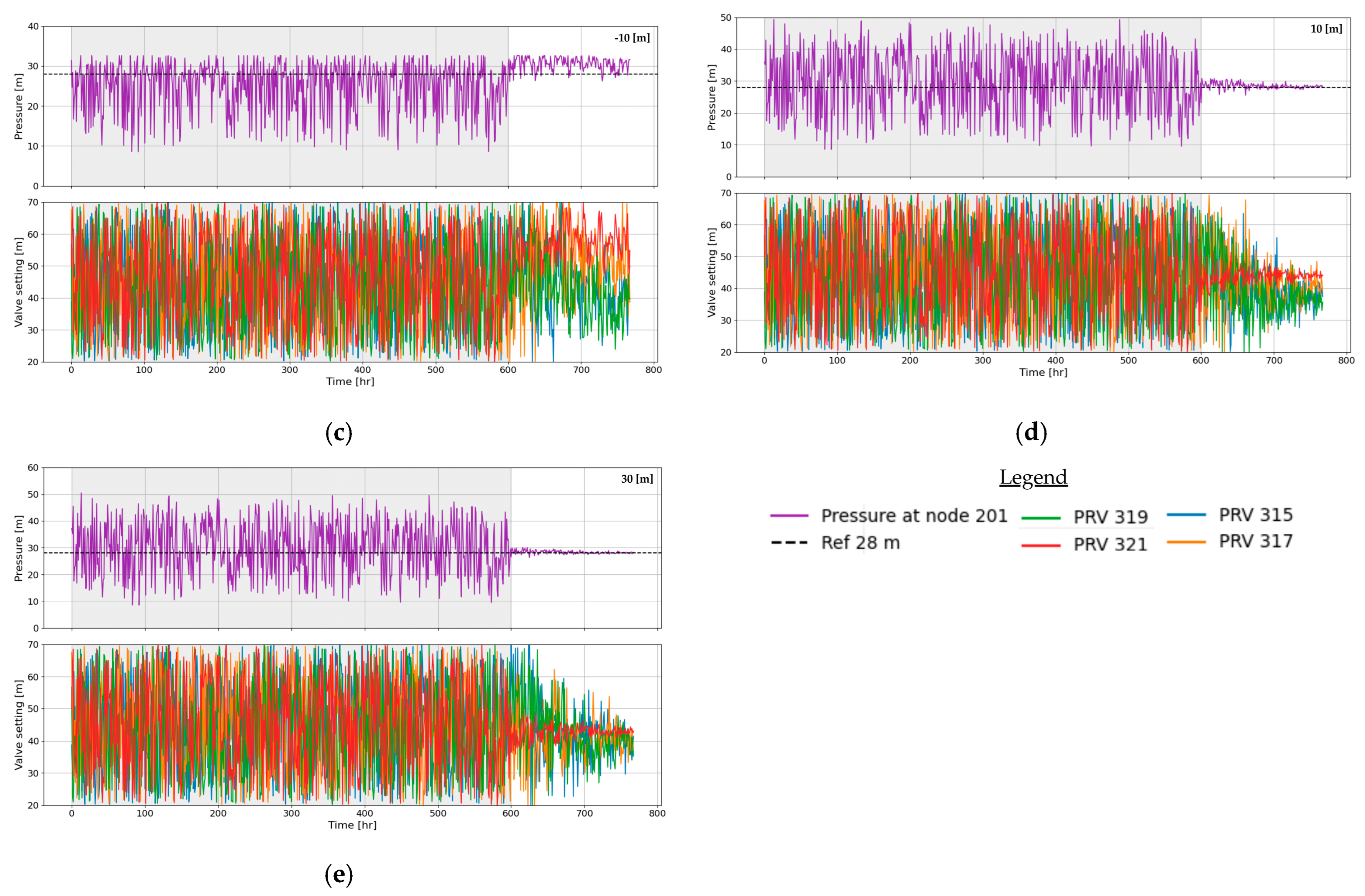
Sensitivity of control performance to reservoir head levels using DeePC. In each panel, the top plot shows the pressure at Node 201 over time (dashed line = 28 [m] reference). The bottom plot shows the valve settings [m] of the pressure-reducing valves (PRVs). The grey segment indicates the randomized data-collection/identification phase, and the white segment indicates the closed-loop control phase. In each run, a uniform offset Δh [m] was applied to the heads of all reservoirs relative to their baseline values. The panels present a representative subset of the tested offsets. (a) Δh = −25 [m]; (b) Δh = −15 [m]; (c) Δh = −10 [m]; (d) Δh = +10 [m]; (e) Δh = +30 [m]. The legend below the panels maps colors to the active valves and indicates the pressure reference line.
In several negative runs, the monitored node pressure remains below the 28 [m] reference throughout the control phase, indicating that the reference is not fully attainable under the reduced supply head. Accordingly, even when PRVs move toward larger openings, the controller’s ability to recover the reference is limited by the boundary conditions, and MAE is therefore used here as a uniform tracking metric while noting the service feasibility limitation. More specifically, for (panels a–c), the pressure remains below the 28 [m] reference for extended periods and does not cleanly converge, and several valve traces are out of bounds or stick to the upper limit, indicating valves that are nearly fully open and thus have limited direct leverage on the node pressure. In contrast, for (panels d–e), settling to the reference is faster, followed by oscillations of relatively small amplitude. Using the legend colors, one can identify the more/less active valves in each case, and traces near the upper bound denote nearly open valves with minor effect, whereas traces at moderate, varying levels indicate active participation in control.
Table 2 compiles the reservoir heads obtained for each tested and confirms a uniform offset across all reservoirs. For example, yields 72, 73.8, 73, and 74.5 [m], and yields 127, 128.8, 128, and 129.5 [m]—i.e., the same baseline heads plus/minus . Beyond validating the setup, these numbers anchor the physical scale, and a range of ≈70–130 [m] is plausible for an urban water network (reservoir heads reflecting topography and friction losses). Hence, [m] represents a large change (≈25% of the baseline head), whereas [m] is moderate. This aligns with performance; low-head scenarios () coincide with weaker control and higher MAE in Figure 9a–c, whereas increased head () is associated with faster settling and lower MAE in Figure 9d,e. Listing the reservoir IDs ensures the scenarios are fully reproducible.
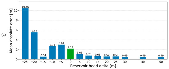
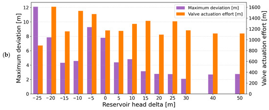
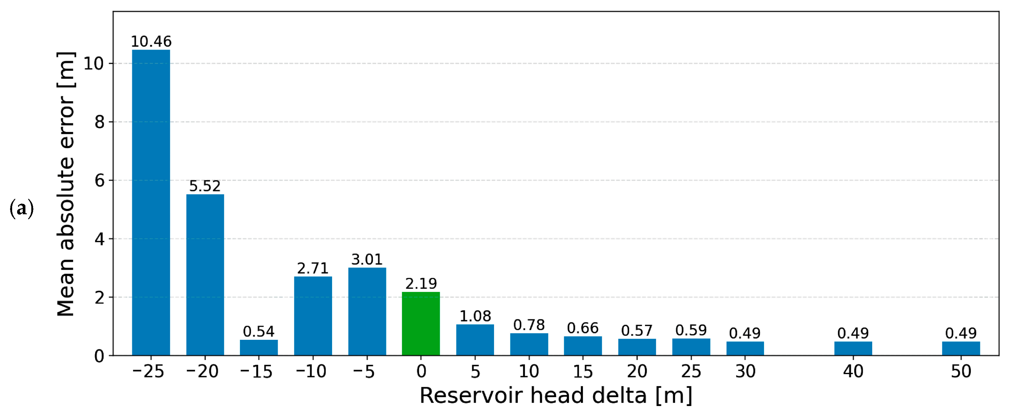
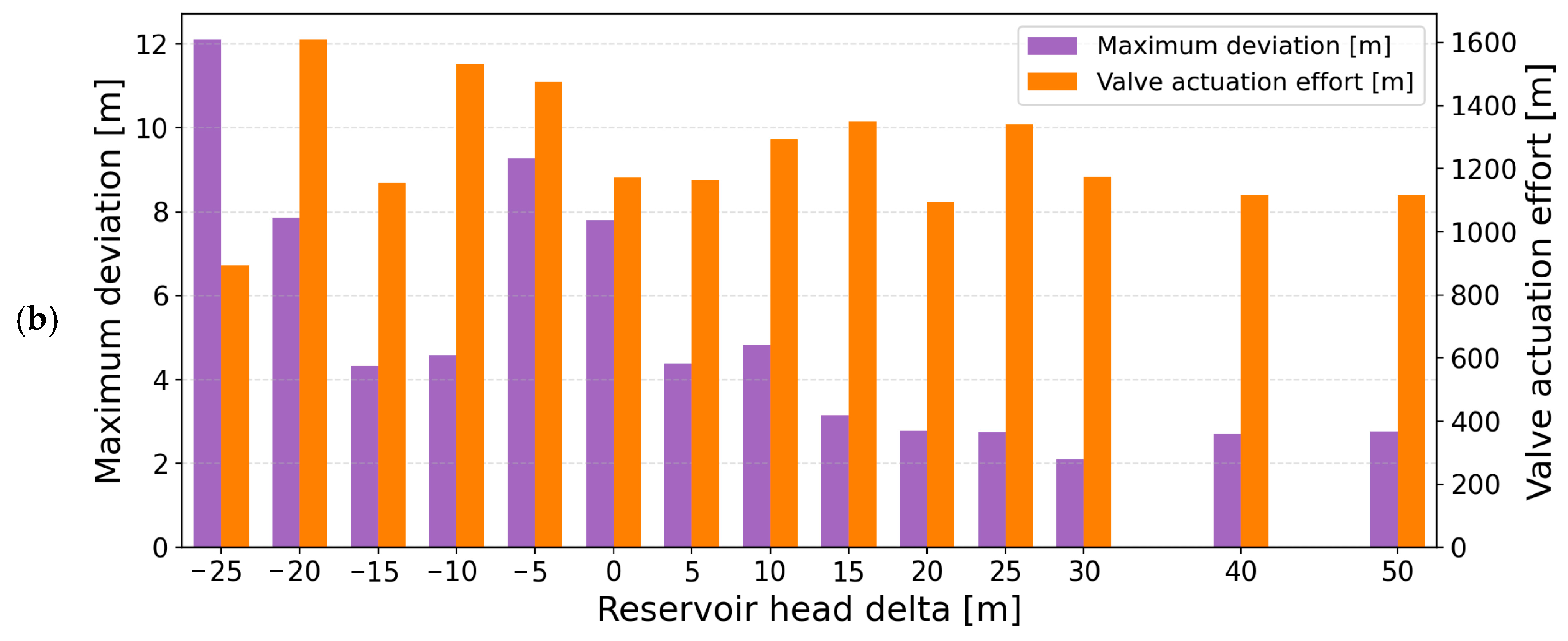
As shown in Figure 10a, the overall trend shows decreasing MAE as increases, but there are notable exceptions on the negative side, as both (0.54 [m]) and (2.71 [m]) yield lower errors than (3.01 [m]), contrary to the general pattern. For positive offsets, a performance floor emerges, and values become nearly constant at about 0.49 [m] starting around . Since no points were tested between +25 and +30, the onset of this plateau occurs somewhere in that interval, but its exact location cannot be determined from the present sampling. Figure 10b complements the tracking results by reporting the maximum deviation and the valve actuation effort for the same reservoir-head offsets. Both metrics show substantial sensitivity for negative , while for sufficiently large positive offsets, the system exhibits consistently low maximum deviations together with a relatively stable actuation demand. Overall, the positive-offset regime that yields the MAE plateau is also associated with comparatively steady behavior in both maximum deviation and actuation effort.
Figure 10.
Sensitivity to a uniform reservoir-head offset () applied to all reservoirs under identical control settings. (a) Mean absolute error of the pressure at Node 201 relative to the 28 [m] reference (y-axis) as a function of reservoir head (x-axis), the baseline case ( = 0) is highlighted in green. (b) Maximum deviation (left y-axis) and valve actuation effort (right y-axis) for the same values.
Table 2.
Resulting reservoir heads [m] after applying a uniform head difference [m] to all reservoirs. For each case (as shown in Figure 11), the reservoir IDs and the resulting head values [m] are reported.
3.2.4. DeePC Regularization Weights
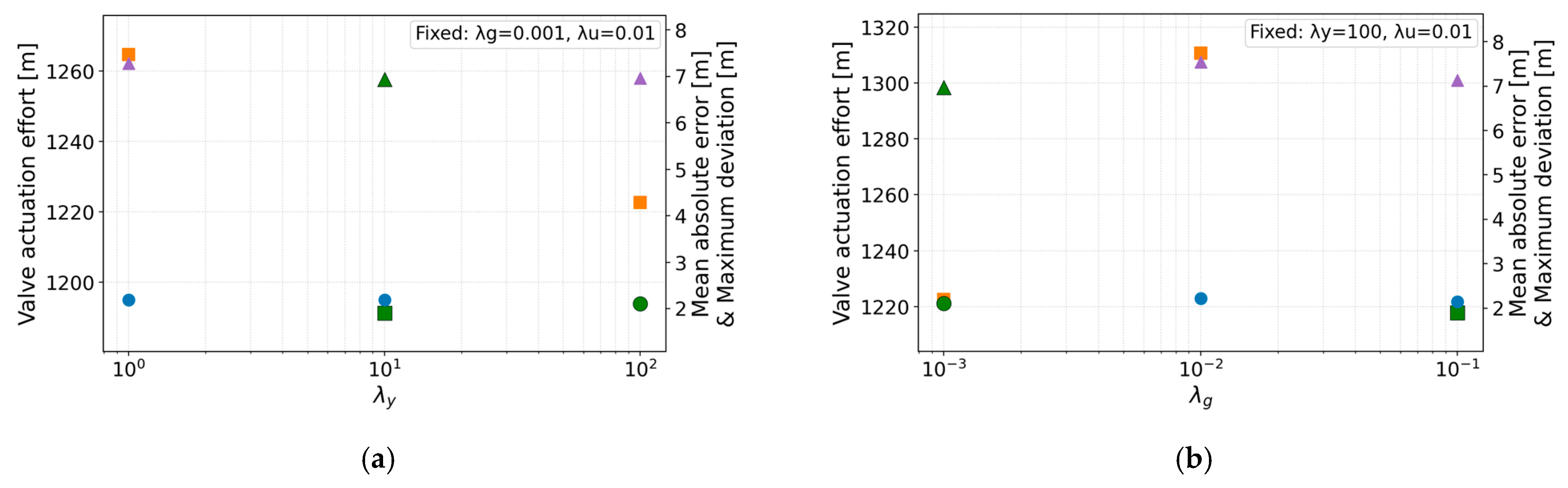
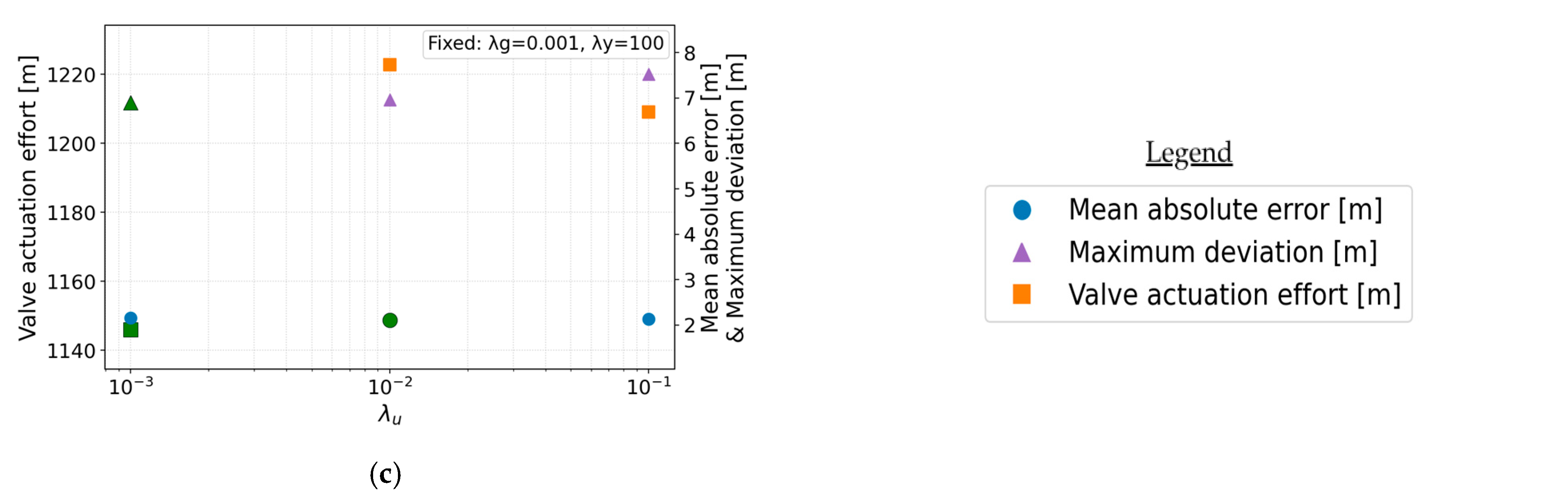
Figure 11 reports the sensitivity of the DeePC regularization weights on the tracking performance at Node 201, varying one weight per panel while keeping the others fixed (as indicated). In the visualization, the three metrics are shown simultaneously using different marker shapes—MAE, maximum deviation, and valve actuation effort—and, for each metric, the lowest observed value within the tested settings is highlighted by coloring that marker in green. Within the sampled ranges, the spread in MAE is modest (≈0.1 [m] between worst and best) and smaller than the effects observed in the other sensitivity studies on this network (e.g., control time-step and reservoir-head changes). Among the tested settings, the lowest value occurred for yielding MAE ≈ 2.11 [m]. Given the sparse, representative sampling, we refrain from inferring global trends. Any further gains would likely require a broader, systematic sweep.
Figure 11.
Sensitivity of the DeePC regularization weights . In each panel, the x-axis (log scale) shows three representative values of the varied weight, while the other two weights are held fixed (reported inside each panel). The y-axis reports valve actuation effort on the left axis and MAE and maximum deviation on the right axis (all in meters). Marker shapes follow the legend: circles—MAE, triangles—maximum deviation, squares—valve actuation effort. For each metric, the marker corresponding to the lowest value among the tested settings is highlighted in green. (a) Varying with and ; (b) varying with and ; (c) varying with and .
4. Discussion
Prior work using optimization algorithms has established that optimally locating pressure-reducing valves (PRVs) can be crucial for regulating pressures in water distribution systems, reducing leakage, and even enabling energy savings (and recovery) [1,5]. Motivated by these findings, we examined how PRV placement interacts with the DeePC method and whether different PRV locations can improve its performance. The analyses on the two networks, Fossolo and Modena, show that adding a PRV can substantially improve tracking of the pressure reference at the monitored node; however, the benefit depends strongly on the added valve’s location and on the local hydraulics.
In the Fossolo network (Figure 1), there was a tendency for topologically closer locations to the monitored node to yield a lower MAE, both when Node 21 was monitored and when the experiment was repeated with Node 15. Still, exceptions were observed, hinting at the role of dominant flow paths. To prove this, we tested two simple indicators: the pipe flow magnitude and the pipe headloss where the PRV was installed. Neither exhibited a clear relation to the resulting MAE, suggesting that dominant paths are not captured by these indicators alone.
In the Modena network (Figure 5), the “closeness” pattern did not persist. The best location was found not at the pipe closest to the monitored node but rather near one of the reservoirs, consistent with the first placement identified by the algorithm reported by Price et al. [3], where the added valve exerted significant control over a large sub-network with downstream surplus pressures. By contrast, locations immediately adjacent to the monitored node (Pipes 274 and 275) did not outperform the baseline. This reinforces that there is no universal rule for PRV placement. To find a DeePC-enhancing location, one must run a brute force search on small networks or rely on an external optimization procedure on larger ones. In addition, Table 1 compares the baseline Modena configuration to the best-performing configuration with one additional internal PRV (Pipe 312). The added internal PRV improves the primary tracking metric, reducing MAE from 2.19 [m] to 2.02 [m]. However, this improvement is accompanied by a higher valve actuation effort and a slightly larger maximum deviation, indicating a clear trade-off between average tracking accuracy and control effort and occasional excursions. A plausible explanation is that introducing an additional degree of freedom allows DeePC to “work harder” (more frequent/larger adjustments distributed across valves) to reduce the average error, even if it does not simultaneously reduce peak deviations.
Figure 3 further indicates that when two valves operate simultaneously, one valve may become dominant while the other remains nearly wide open with little effect. In the worst Fossolo case, the original reservoir valve was mostly at high settings (i.e., largely open), whereas the added valve governed most of the control action, leading to less stable tracking and a higher MAE. This observation is consistent with Price et al. [3], who underscore the strategic importance of the reservoir-adjacent valve for pressure regulation, as a nearly fully open reservoir valve effectively mimics the absence of a regulating valve at that location. The Modena comparison in Table 1 is consistent with this interaction perspective, adding an internal valve can shift and intensify the control action rather than simply “adding regulation for free,” which helps explain why lower MAE may coincide with increased actuation effort.
Regarding controller parameters, a shorter control time step consistently improved performance. Reducing the step increases the number of control iterations within a fixed window, as seen in Figure 7, and convergence to the reference within the window is faster for smaller steps. Consequently, the MAE, an average over the control window, puts greater weight on the many post-convergence samples (with smaller oscillations) as the step decreases. A similar monotonic trend is also observed for the valve actuation effort: as the time step increases, the actuation effort increases as well (Figure 8). This is consistent with the valve and pressure trajectories in Figure 7, where after convergence the pressure fluctuations reduce, and the control actions become more stable; therefore, using a smaller step effectively yields a larger portion of post-convergence “steady” samples within the fixed window, which reduces both the averaged tracking error and the averaged actuation effort. Notably, the maximum deviation remained identical across all tested time steps (7.8 [m]). This supports the interpretation that a single “worst” transient segment occurring early in the control phase dominates the peak error, while the remainder of the window becomes progressively less oscillatory. As a result, changing primarily affects the average metrics (MAE and actuation effort) through the growing proportion of post transient samples, but does not increase the observed peak beyond that early worst-case value. Based on this behavior, we anticipate that continued reductions in the time step will approach a practical error floor at which the MAE stabilizes. In our sampled range, both MAE and actuation effort exhibit an approximately linear trend with the time step (Figure 8). Interestingly, the MAE improvement across the examined steps was approximately linear (Figure 8), which is notable because the time step is an algorithmic choice in DeePC rather than a network-specific characteristic.
Reservoir head levels had a particularly strong effect (Figure 9 and Figure 10a,b). The sensitivity analysis shows that the available hydraulic energy at the sources directly impacts control quality and MAE at the monitored node. In line with Wagner et al.’s results on service-level criteria and head sufficiency at supply nodes [11], insufficient head leads to degraded service, which manifests as worse control performance. In Figure 10a, increasing the head relative to baseline improved tracking up to an apparent plateau between +25 and +30 [m]. Conversely, large decrements severely degraded performance due to a lack of “hydraulic power.” These results stress the need to calibrate the system before running DeePC so that the controller is assessed under meaningful operating conditions. The non-monotonic behavior seen for −15 [m] and −10 [m] (Figure 9b,c), a drop, then a rise, stems from the network lacking sufficient head to drive flow to the monitored node. The measured pressure exhibits very small oscillations tightly near the 28 [m] reference from below. Figure 9a shows a related case where the pressure does not approach the reference at all. Altogether, these findings indicate a practical improvement limit and the importance of calibrating reservoir heads prior to control. In addition to MAE, Figure 10b complements the interpretation by reporting maximum deviation and valve actuation effort. Unlike the largely monotonic MAE trend (Figure 10a), these two metrics do not exhibit a single clear monotone pattern across . For the most negative offsets (and around −5 [m]), the maximum deviation becomes relatively large, consistent with a “struggle” regime in which the controller attempts to compensate for insufficient hydraulic head. Importantly, the relatively low MAE observed at −15 and −10 [m] should therefore be interpreted cautiously, as, despite low average error, the pressure can remain “stuck” near the reference from below due to head insufficiency, so the MAE may reflect a constrained operating point rather than genuinely improved controllability. For positive offsets, the decrease in maximum deviation from about −5 [m] toward higher heads is consistent with easier regulation as more head becomes available; however, beyond roughly +30 [m], the actuation effort curve suggests a shallow optimum rather than a strict plateau, with the lowest effort occurring around the +30 [m] case and a slight increase thereafter. This indicates that while higher heads can improve MAE, they do not necessarily minimize control effort, and a practical operating point may be better selected by balancing the three metrics. Finally, the actuation effort metric appears most informative once the valves begin actively modulating (rather than remaining near a saturated “mostly open” behavior under severe head deficit), which is consistent with the time series behavior in Figure 9.
Finally, the tuning of regularization weights modestly affected performance compared to the other sensitivities. Good operating points were found, but no dramatic changes between neighboring values. Following Coulson et al. [7], we selected the tested ranges, and, within them (Figure 11a–c) we observed the following: (i) higher λᵧ improved tracking; (ii) a relatively small λg yielded the lowest MAE, while larger values degraded performance; and (iii) for λu, there was an interior best value, with too small or too large values worsening MAE. The meaning of these choices follows the guidance in Coulson et al.’s work [7]. In Figure 11a–c, the same qualitative conclusion holds for the maximum deviation, which shows similarly mild sensitivity, indicating that pressure oscillations are not strongly amplified by neighboring regularization settings within the tested grid. In contrast, the valve actuation effort exhibits a clearer dependence on the regularization weights, suggesting that the tuning primarily changes how “aggressively” the controller uses the valves rather than fundamentally altering the achievable tracking quality. This is consistent with the role of the regularizers, particularly λu, which directly penalizes the control sequence and therefore affects how strongly the optimizer modulates the PRVs, while λᵧ and λg can also influence effort indirectly by changing the preferred trajectory fit and the regularization of the DeePC decision variables [7]. Across the sampled combinations, some cases show overlap between the best-performing settings of different metrics (as indicated by the green-highlighted markers per metric), but this is not systematic in such a sparse grid. Overall, these results suggest that once reasonable ranges are selected (per Coulson et al. [7]), the final choice of regularization weights may benefit from placing additional emphasis on valve actuation effort, which appears more discriminative here, while acknowledging the inherent trade-off between the three objectives. A broader and denser sweep would be needed to confirm whether the observed overlaps persist and to identify robust multi-metric settings.
5. Conclusions
This study shows that DeePC performance in water distribution systems is sensitive to operating conditions and therefore should be preceded by baseline calibration of the system (especially reservoir-head conditions) to avoid biased, artificially bounded, or unreliable outcomes and to realize the controller’s potential. Across the sensitivities we examined, PRV placement, control time step, reservoir head, and regularization weights, we observed performance gains when an additional PRV was placed at favorable locations, the control time step was reduced, and the reservoir head was sufficient to supply the required hydraulic power. The tuning of regularization weights had a measurable but comparatively modest effect. The results should be interpreted as local, baseline-anchored sensitivities because we varied one factor at a time while holding the others fixed. Potential cross-factor interactions (e.g., , PRV placement) were outside the present scope and are a natural direction for future work. In addition to that, additional factors may also be relevant and warrant systematic investigation. We found that the sensitivity-driven improvements are not limited to MAE, depending on the operating condition, maximum deviation, and valve actuation effort, and can either improve alongside MAE or reveal trade-offs (e.g., improved tracking at the expense of higher actuation effort when adding an internal PRV). Across both benchmark networks, DeePC achieved repeatable closed-loop tracking of a fixed pressure reference using only measured input–output data and valve constraints, and its performance responded consistently to hydraulically meaningful changes. In Fossolo, several internal PRV placements reduced the baseline MAE, whereas unfavorable placements markedly increased the error, demonstrating that DeePC can both benefit from and diagnose structural controllability differences within the network. In Modena, the best tested candidate improved the baseline MAE, and time-step refinement yielded a consistent MAE reduction over the examined range. Moreover, consistent with the MAE trend under time-step refinement, the valve actuation effort decreased as the time step decreased, indicating that improved tracking was accompanied by less aggressive control action over the stabilized portion of the window. Reservoir-head offsets had a pronounced, physically interpretable effect: increasing heads improved tracking until a plateau, while negative offsets degraded performance. Finally, the comparatively modest spread observed under the tested regularization weight settings indicates that, once baseline hydraulic conditions are plausible, DeePC can deliver stable pressure control without requiring excessively delicate tuning. At the same time, the actuation effort metric was more sensitive than the pressure error metrics to changes in regularization weights, suggesting that once a reasonable range is selected, practical tuning can prioritize effort/operability without substantially compromising tracking. As a concrete next step, we propose an outer loop genetic-algorithm optimization that searches over candidate PRV locations, using DeePC-in-the-loop experiments to score each candidate and select the placement that minimizes the tracking error. Future work should also extend the performance assessment beyond a single monitored node by incorporating spatial service metrics (e.g., network-wide pressure compliance and spatial pressure variability) to ensure that improved local tracking does not come at the expense of degraded conditions elsewhere in the network.
Author Contributions
Conceptualization, J.D.; methodology, J.D.; software, J.D.; validation, J.D.; formal analysis, J.D.; investigation, J.D.; data curation, J.D.; writing—original draft preparation, J.D.; writing—review and editing, J.D. and A.O.; visualization, J.D.; supervision, A.O.; funding acquisition, A.O. All authors have read and agreed to the published version of the manuscript.
Funding
This research was supported by the Israeli Water Authority under project number 2033800, and by the Bernard M. Gordon Center for Systems Engineering at the Technion.
Data Availability Statement
The original contributions presented in this study are included in the article. Further inquiries can be directed to the corresponding author.
Conflicts of Interest
The authors declare no conflicts of interest.
Abbreviations
The following abbreviations are used in this manuscript:
| DeePC | Data-Enabled Predictive Control |
| MAE | Mean Absolute Error |
| PRV | Pressure-Reducing Valve |
| WDS | Water Distribution Systems |
| RTC | Real-Time Control |
| MPC | Model Predictive Control |
Appendix A
Table A1.
Baseline parameters and evaluation settings.
Appendix B. Raw Results of the Sensitivity Analyses
Table A2.
Relative to the 28 [m] reference, under identical identification and control settings. In each run, the additional PRV was installed on the pipe listed in the row, while all other settings were kept unchanged. The table enables a direct ranking of candidates.
Table A3.
Raw results of the uniform reservoir-head offset sensitivity analysis. The table reports three performance metrics: mean absolute error of the controlled node pressure (Node 201) relative to the reference, maximum deviation from the reference, and valve actuation effort during the control phase (in meters).
Table A4.
Raw results of the control time-step sensitivity analysis. For each , control was executed over a fixed duration of h, such that the number of control updates varies with the time step. The table reports three performance metrics: mean absolute error of the controlled node pressure (Node 201) relative to the reference, maximum deviation from the reference, and valve actuation effort, normalized by the control-phase duration to enable a consistent comparison across different values.
References
- Morani, M.C.; Carravetta, A.; D’Ambrosio, C.; Fecarotta, O. A new mixed integer non-linear programming model for optimal PAT and PRV location in water distribution networks. Urban Water J. 2021, 18, 394–409. [Google Scholar] [CrossRef] [Scilit]
- Rajakumar, A.G.; Cornelio, A.A.; Kumar, M.S.M. Leak management in district metered areas with internal-pressure reducing valves. Urban Water J. 2020, 17, 714–722. [Google Scholar] [CrossRef] [Scilit]
- Price, E.; Abhijith, G.R.; Ostfeld, A. Pressure management in water distribution systems through PRVs optimal placement and settings. Water Res. 2022, 226, 119236. [Google Scholar] [CrossRef] [Scilit] [PubMed]
- Perelman, G.; Ostfeld, A. Data Enabled Predictive Control for Water Distribution Systems Optimization. Water Resour. Res. 2025, 61, e2024WR039059. [Google Scholar] [CrossRef] [Scilit]
- Maurizio, G.; Nicola, F.; Antonio, R. Optimal Location of PRVs and Turbines in Water Distribution Systems. J. Water Resour. Plan. Manag. 2014, 140, 06014004. [Google Scholar] [CrossRef] [Scilit]
- Zhang, X.; Zhang, K.; Li, Z.; Yin, X. Deep DeePC: Data-enabled predictive control with low or no online optimization using deep learning. arXiv 2024, arXiv:2408.16338. [Google Scholar] [CrossRef] [Scilit]
- Coulson, J.; Lygeros, J.; Dörfler, F. Data-Enabled Predictive Control: In the Shallows of the DeePC. arXiv 2019, arXiv:1811.05890. [Google Scholar] [CrossRef] [Scilit]
- Elokda, E.; Coulson, J.; Beuchat, P.N.; Lygeros, J.; Dörfler, F. Data-enabled predictive control for quadcopters. Int. J. Robust Nonlinear 2021, 31, 8916–8936. [Google Scholar] [CrossRef] [Scilit] [PubMed]
- Coulson, J.; Lygeros, J.; Dörfler, F. Distributionally Robust Chance Constrained Data-enabled Predictive Control. arXiv 2021, arXiv:2006.01702. [Google Scholar] [CrossRef] [Scilit]
- Huang, L.; Zhen, J.; Lygeros, J.; Dörfler, F. Robust Data-Enabled Predictive Control: Tractable Formulations and Performance Guarantees. arXiv 2021, arXiv:2105.07199. [Google Scholar] [CrossRef] [Scilit]
- Wagner, J.M.; Shamir, U.; Marks, D.H. Water Distribution Reliability: Simulation Methods. J. Water Resour. Plan. Manag. 1988, 114, 276–294. [Google Scholar] [CrossRef] [Scilit]
- Willems, J.C.; Rapisarda, P.; Markovsky, I.; De Moor, B.L.M. A note on persistency of excitation. Syst. Control Lett. 2005, 54, 325–329. [Google Scholar] [CrossRef] [Scilit]
- Fossolo. Available online: https://waterfutures.github.io/WaterBenchmarkHub/benchmarks/network-Fossolo.html (accessed on 1 December 2025).
- Modena. Available online: https://waterfutures.github.io/WaterBenchmarkHub/benchmarks/network-Modena.html (accessed on 1 December 2025).
- Kyriakou, M.S.; Demetriades, M.; Vrachimis, S.G.; Eliades, D.G.; Polycarpou, M.M. EPyT: An EPANET-Python Toolkit for Smart Water Network Simulations. J. Open Source Softw. 2023, 8, 5947. [Google Scholar] [CrossRef] [Scilit]

Disclaimer/Publisher’s Note: The statements, opinions and data contained in all publications are solely those of the individual author(s) and contributor(s) and not of MDPI and/or the editor(s). MDPI and/or the editor(s) disclaim responsibility for any injury to people or property resulting from any ideas, methods, instructions or products referred to in the content. |
© 2026 by the authors. Licensee MDPI, Basel, Switzerland. This article is an open access article distributed under the terms and conditions of the Creative Commons Attribution (CC BY) license.