


Abstract
Evapotranspiration (ET) forecasts from the U.S. National Water Model (NWM) carry systematic biases that are most apparent in water-stressed, intensively managed regions. This study develops a machine learning (ML) post-processing framework that bias-corrects 1–7 day accumulated ET (ACCET) forecasts from the NWM medium-range configuration using NWM meteorological forcings, the raw NWM-ACCET forecast, and auxiliary spatial and temporal predictors. Three tree-based models—Random Forest (RF), XGBoost, and LightGBM—were trained on AmeriFlux eddy-covariance observations at four California model-development sites and evaluated using nested five-fold temporally blocked cross-validation with a ±7-day purge window; two additional sites were withheld for independent off-site validation. All three models substantially outperformed the raw NWM forecasts. Pooled out-of-fold performance across the four model-development sites yielded values of 0.832–0.854 and mean-normalized root mean squared error (NRMSE) values of 0.427–0.460, compared with = 0.086 and NRMSE = 1.206 for the raw NWM forecasts. LightGBM and XGBoost were favored over RF in this four-site out-of-fold evaluation. Independent off-site validation yielded values of 0.796–0.874 and NRMSE values of 0.380–0.459, with RF showing the most robust overall performance. Converting ACCET to lead-time-specific increments revealed substantially stronger lead-time degradation than was apparent from the accumulated metrics. Feature-importance and SHapley Additive exPlanations (SHAP) analyses identified wind, lead time, seasonality, and radiation as dominant predictors. The framework offers a practical route to more reliable operational ET forecasts for water management, agriculture, and drought monitoring, with potential for extension to climatically similar regions.
1. Introduction
Evapotranspiration (ET) is a major component of the water balance in any watershed. Approximately 70% of precipitation on land surfaces returns to the atmosphere through ET [1]. ET is an essential parameter in hydrologic models used for forecasting river stages, flood potential, drought, groundwater recharge, and irrigation schedules, as it directly affects surface runoff [2,3,4]. Accurate ET information also supports crop-yield prediction and food security, with significant implications for regional agricultural economies [5].
Various approaches, including hydrological models, land surface models (LSMs), and remote-sensing techniques, have been developed to simulate or estimate actual ET. Eddy-covariance (EC) measurements are widely regarded as one of the most accurate footprint-scale methods for quantifying turbulent water-vapor and energy fluxes between the land surface and atmosphere. They therefore provide direct observations for evaluating large-scale ET products [6]. Among large-scale approaches, remote sensing and LSMs produce global or continental-scale ET datasets. However, these large-scale datasets may not provide accurate ET values for an area of interest, as their accuracy and uncertainty vary spatially based on the input and model algorithms [7]. In the United States (US), the National Oceanic and Atmospheric Administration’s (NOAA) National Water Model (NWM) is a continental-scale hydrologic model that produces streamflow forecasts across 2.7 million reaches and also provides continuous ET forecasts with various lead times at 1 km spatial resolution across the Continental United States (CONUS), Hawaii, Alaska, and Puerto Rico [8].
The NWM uses the Noah-MP land surface model to simulate land-surface variables such as ET, soil moisture, and snowpack, alongside streamflow-related outputs [9,10]. It provides both multi-year retrospective simulations of historical conditions and continuously updated operational forecasts.
Operational forecasts are issued as short-range, medium-range, and long-range products. Short-range forecasts provide high-temporal-resolution predictions over shorter horizons of up to 18 h, whereas medium-range and long-range forecasts extend to 10 days and 30 days, respectively. For ET applications, medium-range forecasts provide a practical forecast horizon for near-term water resources, agricultural, and drought-monitoring decisions [11,12,13]. Because ET is often used in accumulated form for irrigation scheduling and water-balance decisions, medium-range accumulated ET forecasts can provide practical information for near-term agricultural water management [14,15,16]. NWM medium-range forecasts are driven by meteorological forcing data derived from the Global Forecast System (GFS), a numerical weather prediction system operated by the National Weather Service [17,18]. Each forecast cycle uses forcings available at initialization [8].
Previous evaluations of the NWM have primarily focused on retrospective products, including streamflow simulations [19,20,21,22,23], snow-related outputs [24], soil moisture and evaporative demand products [25], and ET simulations [26,27]. Fewer studies have assessed operational NWM forecasts, with existing work focusing mainly on streamflow and flood performance [13,28,29,30,31]. Consequently, despite their relevance for near-term water-resource and agricultural decisions, operational NWM medium-range ET forecasts and their ML-based post-processing remain largely underexplored.
Hydrological models, including the NWM, have uncertainties originating from their simplified representations of complex systems, which can reduce the accuracy of simulations [32]. Evaluations of the NWM’s performance across the CONUS consistently highlight specific regions where the model underperforms in simulating variables such as streamflow, soil moisture, and ET [19,21,25,26,27,31]. A CONUS-scale evaluation by Abdelkader et al. [19] identified problems with NWM retrospective streamflow performance in arid and semi-arid regions. Johnson et al. [21] found the NWM to exhibit reduced performance in arid regions and noted that biases in input data, such as precipitation, can significantly affect water-balance components, resulting in lowered accuracy. Consistent with these broader water-balance concerns, ET-focused evaluations have also identified biases in NWM retrospective products. Nassar et al. [27] analyzed NWM retrospective ET alongside the OpenET models [33] and found underprediction bias in irrigated agricultural lands, riparian areas, and wetlands. Chapagain et al. [26] conducted a CONUS-scale evaluation of NWM v3.0 retrospective ET using eddy-covariance observations and identified a significant negative bias in the California–Nevada River Forecast Center (RFC) region, the largest among all RFC regions. Together, these ET-focused findings indicate that NWM ET biases are regionally structured and relevant to water-managed landscapes. Given the documented negative ET bias and intensive water-management needs in the California–Nevada RFC region, this region provides a suitable test area for developing and evaluating bias-correction approaches for NWM ET forecasts.
Several factors likely influence ET simulation accuracy within the NWM framework. The NWM does not represent sub-grid variability, which can introduce biases in regions with complex topography and varied land use [8]. Consequently, sub-grid practices such as irrigation and other anthropogenic activities are difficult to represent. Currently, there is no calibration for NWM variables except streamflow. NWM streamflow forecasting employs sophisticated techniques such as data assimilation to refine predictions [34]. However, similar corrections do not benefit other forecasted hydrological variables, including ET. As a result, biases can persist and limit their applicability.
Several approaches are available to correct model biases, including parameter calibration, improved forcing data to better represent heterogeneous processes, and post-processing (i.e., bias correction) of NWM outputs. Post-processing can be implemented without altering the model framework and tailored for specific regions or applications. Traditional bias-correction methods include linear scaling, quantile mapping, distribution mapping, and ensemble techniques [35]. Although these methods can correct biases in historical or retrospective simulations, their performance for forecast data may be limited by evolving error characteristics and the assumption of stationary bias relationships [36]. Machine learning (ML) has become a widely used data-driven approach to bias correction and hydrologic prediction. ML approaches have shown promising results for bias correction in ET modeling [37,38,39,40]. Previous studies have established the effectiveness of ML-based post-processing of NWM retrospective simulations and forecasts, particularly for streamflow [41,42,43]. However, ML-based post-processing has been applied mainly to NWM streamflow products, while its use for bias-correcting NWM ET forecasts remains largely unexplored.
A wide variety of ML models from neural-network, tree-based, kernel-based, and hybrid approaches have been explored for bias-correction and forecasting applications in hydrology and water resources [44,45]. Deep learning models, including long short-term memory networks (LSTM) and convolutional neural networks (CNN), are widely used in hydrology for time-series and spatial remote-sensing applications, respectively [45,46,47]. However, tree-based models, including Random Forest (RF), Extreme Gradient Boosting (XGBoost), and Light Gradient Boosting Machine (LightGBM) remain competitive because of their relatively low computational cost, faster training, and robustness to non-informative features, with strong performance on tabular data [48]. Recent advancements in boosting algorithms, such as XGBoost, have further improved their performance and applicability in hydrologic forecasting [49].
Accordingly, this study develops and evaluates a tree-based ML framework for bias-correcting NWM medium-range ET forecasts using hydrometeorological and temporal features, extending the ML post-processing analysis first reported in the first author’s M.S. thesis [50]. The analysis focuses on the California–Nevada RFC region, where persistent ET biases have been identified. Using RF, XGBoost, and LightGBM, the study assesses the effectiveness of ML-based bias correction, compares model performance, examines the effects of forecast lead time and predictor importance, and provides an initial assessment of off-site performance at nearby sites with similar hydroclimatic characteristics. To our knowledge, this is the first peer-reviewed study to develop ML-based post-processing for operational NWM medium-range ET forecasts.
2. Materials and Methods
2.1. Study Area
Six EC tower sites within the California–Nevada RFC region were selected for this study (Figure 1). The six selected sites are grouped into three spatial clusters, each consisting of a pair of nearby locations. Four sites (US-Myb, US-Sne, US-Ton, and US-Var) were used as training sites for model fitting and temporally blocked cross-validation, while two sites (US-Tw1 and US-Tw4) were reserved for independent validation. All sites are located within the Csa Köppen climate zone, characterized by a temperate climate with hot, dry summers. The sites include a mix of land cover types, including cultivated croplands, wetlands, and shrub/scrub areas, as summarized in Table 1. The broader region plays a critical role in California’s agricultural productivity and water resource management [51], but is also prone to recurrent droughts, with increasing severity under changing climate conditions.
Figure 1.
Study sites in California, showing training and validation sites.
Table 1.
Study sites with corresponding coordinates, elevation, and National Land Cover Database (NLCD) land cover. All sites are in the Csa Köppen climate zone.
2.2. Features and Data
2.2.1. Overview
The NWM forcings are connected to the simulated ET through physics-based equations implemented in the NWM framework. This underlying connection makes them suitable for being considered supplementary ML features alongside NWM ET. The use of such variables as ET predictors is also prominent in the broader literature. The relationship between ET and solar radiation, wind speed, and temperature variables has been used as features in various ML prediction models for ET, demonstrating that including these variables improves performance [52,53]. Pagano et al. [53] used an RF model to predict daily ET values in a citrus farm under controlled irrigation conditions and found solar radiation to be one of the most significant features. Zhao et al. [54] used four tree-based ML models—RF, extremely randomized trees, XGBoost, and LightGBM—to estimate terrestrial ET, and found that net radiation was the most important feature. Hu et al. [55], who used SHapley Additive exPlanations (SHAP) analysis to characterize their ET prediction models, including deep neural network (DNN), RF, and symbolic regression (SR), found net radiation, air temperature, and land surface temperature to be orderly significant model features. Babaeian et al. [56] found wind speed to be an important input to an LSTM model, along with temperature and radiation. The strong influence of these variables as key ML features is consistent with their physical roles in driving ET processes.
Auxiliary features can complement physically based variables to enhance model performance. ET exhibits a strong seasonal cycle, which ML models can exploit. Previous studies have incorporated temporal indicators such as day of year (DoY) [52,53], demonstrating their importance in improving predictive skill. In this study, we represent this seasonality at an hourly scale using the hour of year (HoY) fraction, which captures the relative position of a given time within the annual cycle.
The concept of lead time, defined as the time difference between forecast initialization and prediction time and representing the forecast horizon, has been effectively employed in prior studies both as a feature and as a basis for categorization during model formulation and analysis, particularly in the context of ML predictions in hydrology, such as streamflow [11,57,58,59]. While the land surface variables used in this study are obtained directly from NWM forcings, we augment them with auxiliary spatial and temporal features to improve the model’s ability to capture systematic variability in ET.
For model development, we evaluated predictors from three categories: (1) NWM forcing variables, (2) model-derived accumulated ET predictions from the NWM medium-range forecast (NWM-ACCET), and (3) auxiliary features, including spatial (latitude and longitude) and temporal (lead time and HoY fraction) descriptors. We deliberately include both the raw NWM-ACCET forecast and the forcing variables used to drive it: the framework is designed to correct, rather than replace, the physically based forecast, and retaining the raw forecast lets the models learn its systematic errors as a function of the accompanying meteorological conditions. Because the forcings and NWM-ACCET share information, some redundancy among predictors is expected; its implications for interpreting feature attributions are discussed in Section 2.3.4 and Section 3.2.4. Table 2 summarizes the full set of features used in this study. The variables SWDOWN, LWDOWN, RAINRATE, U2D, V2D, Q2D, T2D, and PSFC represent meteorological forcing inputs used to drive the NWM simulations. In addition, we include predictors based on the NWM-ACCET forecasts, along with lead time, geographic coordinates, and HoY fraction. Here, model initialization time (MIT) refers to the time at which a forecast is initiated, and forecast time (FT) refers to the future time for which the forecast value is produced.
Table 2.
Overview of the feature variables used in the study, including their descriptions, temporal and spatial resolutions, and data sources.
2.2.2. NWM ET Forecasts
The NWM medium-range forecasts provide ET predictions at a native 3-h temporal resolution on a 1 km spatial grid, with forecast horizons extending to approximately 8.5–10 days and updated every 6 h. Within the NWM, ET is computed by the Noah-MP land surface model as actual evapotranspiration: the sum of evaporation of canopy-intercepted water, plant transpiration, and direct soil evaporation [9]. The ACCET variable analyzed in this study represents accumulated total ET and therefore includes all three components. In this study, we focus on the first 1–7 days of the forecast horizon and subsample the data by selecting one initialization per day (00:00 UTC) and sampling values at 24-h lead times (24, 48, …, 168 h), yielding one forecast per day and seven cumulative ET values per forecast. This focus on the first 7 days (168 h) reflects their greater relevance for practical applications and generally higher forecast skill. The NWM underwent significant configuration changes during the two-year study period from 1 January 2019 to 31 December 2020. During 1 January to 18 June 2019, forecasts were generated using the NWM v1.2 single-member configuration, and we used that member directly in our analysis. For the later period, forecasts were produced using the NWM v2.0 ensemble configuration [17], and we used the arithmetic mean of seven ensemble members, assuming equal contributions from each member in representing uncertainty [60], to provide a similar deterministic representation of the forecasts across the study period. While this introduces differences in the statistical characteristics of the forecasts over time, the ML framework is expected to learn and adapt to these variations.
The NWM medium-range forecasts of accumulated total ET (ACCET) are available as gridded data with a 1-km spatial resolution. These data represent ET accumulated from the MIT to each FT. The elapsed time between MIT and FT is the forecast lead time and, for ACCET, also represents the duration over which ET is accumulated.
We retrieved the forecast data as files in Kerchunk Zarr format stored in an Amazon S3 bucket [61] and extracted values corresponding to the grid cells containing each EC tower location. To reduce data complexity, we evaluated one forecast per day by selecting forecasts initialized at 00:00 UTC, as noted earlier, although forecasts are generated every 6 h. For each daily MIT, ACCET values were sampled at 24-h lead times, resulting in cumulative ET values corresponding to increasing accumulation periods within each forecast run (i.e., accumulation resets for each MIT). Figure 2 provides a graphical representation of this process and the resulting dataset.
Figure 2.
NWM-ACCET medium-range forecast data extraction and preprocessing workflow. Forecasts initialized at 00 UTC are selected from the Amazon S3 bucket, and ACCET values are sampled at daily lead times (FT1–FT7), resulting in seven cumulative ET values per forecast. The right panel illustrates the temporal structure of the selected forecasts, where the blue flag marks the model initialization time (MIT), and color shading represents increasing lead time.
2.2.3. NWM Forcing Variables
We downloaded the NWM forcings corresponding to the retrieved medium-range forecast matching the MIT. These data included the 10-m U-component of wind (U2D), 10-m V-component of wind (V2D), 2-m air temperature (T2D), 2-m specific humidity (Q2D), surface pressure (PSFC), surface downward long-wave radiation flux (LWDOWN), surface downward short-wave radiation flux (SWDOWN), and surface precipitation rate (RAINRATE). The forcings are available at hourly temporal resolution and on a 1 km spatial2 grid in the Amazon S3 bucket [61]. For each MIT (00:00 UTC), we extracted the forcings used to produce ACCET at 24-h intervals, extending up to 7 days. The resulting dataset included combinations of MIT and FT, matching the structure of the ACCET data. The extraction and preparation workflow for these data follows the same procedure as for the NWM-ACCET medium-range forecast, as depicted in Figure 2, with values extracted from the grid cells corresponding to each EC tower location.
2.2.4. AmeriFlux Eddy-Covariance Data
The AmeriFlux network in the USA maintains EC towers measuring various flux variables, including latent heat flux, that can be used to compute ET [62]. We used latent heat flux measurements from six AmeriFlux EC tower sites in California for the study period, obtained from the FLUXNET database. FLUXNET is a global initiative that provides quality-controlled and gap-filled flux measurements. The daily mean latent heat flux (LE) data, provided in W/m2, were converted into daily ET (mm/day) using Equation (1) [63]:
where ET is evapotranspiration in mm/day, LE is the latent heat flux in W/m2, is the density of water in kg/m3, and is the latent heat of vaporization in J/kg. The factor 86,400 converts seconds to days, and the factor 1000 converts meters to millimeters. Daily air temperature data from the same AmeriFlux source were used to estimate the temperature-dependent values of and .
Once we computed the ground-truth ET values, we processed them to calculate accumulated ET (EC-ACCET) for each day up to the seventh day, aligning with the extracted NWM-ACCET dataset to match the accumulated nature of the NWM forecasts. The EC-ACCET values served as the ground truth for model training and evaluation. For the primary ML modeling and evaluation, both the target variable and model predictions were treated as ACCET. We selected cumulative ACCET, rather than lead-time-specific daily ET, as the primary prediction target for two reasons. First, ACCET is the quantity natively produced by the NWM medium-range configuration, so correcting it directly preserves a one-to-one correspondence with the operational product. Second, multi-day accumulated ET is the quantity most directly used in irrigation-scheduling and water-balance decisions over medium-range horizons, and correcting the accumulation directly avoids the compounding of errors that occurs when independently corrected daily increments are re-aggregated. Lead-time-specific ET increments were derived only for the supplemental lead-time analysis to distinguish true forecast-horizon effects from the accumulation effect inherent in ACCET.
2.3. Model Development and Evaluation
We trained and evaluated three supervised, tree-based ML models: RF, XGBoost, and LightGBM, using two years of data from four training sites. Two additional sites were reserved for independent off-site validation. Following preliminary feature screening, the final models used NWM-ACCET, HoY fraction, lead time, longitude, latitude, and the NWM forcings U2D, V2D, T2D, Q2D, PSFC, LWDOWN, and SWDOWN as predictors, with EC-ACCET as the target variable. Hyperparameter selection and within-site evaluation were performed using nested five-fold temporally blocked cross-validation with a ±7-day purge window, as described in Section 2.3.3. Figure 3 summarizes the workflow.
Figure 3.
Workflow of the ML-based post-processing framework for NWM-ACCET forecasts, including preliminary feature screening, nested temporally blocked hyperparameter tuning and evaluation, final model fitting, and independent off-site validation.
Across the six sites, 30,534 records were theoretically available after accounting for terminal forecast truncation. Of these, 1596 records (5.227%) were unavailable, leaving 28,938 usable observations. The unavailable records comprised 1050 records associated with 25 initialization dates absent from the compiled source data and 546 (1.8%) records associated with 13 initialization dates for which NWM-ACCET was unavailable across all sites. These unavailable records were excluded before model development and evaluation.
The following subsections describe the ML models, evaluation metrics, nested temporally blocked hyperparameter tuning and cross-validation, feature selection, and SHAP-based interpretation.
2.3.1. Machine Learning Models
RF is an ensemble ML technique in which numerous decision trees are created during model training, and output is produced using a set of predictors [64]. The final output is determined by methods such as averaging the values (for regression) or selecting the mode (for classification) from the individual trees [65]. RF trains multiple decision trees using bootstrapped samples from the original dataset, where each tree is independently trained on a unique subset of data sampled with replacement from the full dataset [66]. RF reduces variance without substantially increasing bias; hence, it is notably robust to overfitting, can effectively capture non-linearity, and uses a relatively small number of parameters, making it easy to use [67]. Additionally, RF demonstrates robust performance without the requirement for data normalization or scaling [68]. RF also has a built-in feature importance function that helps identify influential predictors. The model training was followed by hyperparameter tuning to obtain the optimal parameters for the RF model. We developed the RF model in Python (version 3) for this study using the scikit-learn library [69].
XGBoost is a gradient boosting-based ML algorithm known for its computational efficiency and scalability [70]. It is also known to handle missing values effectively. The objective function in XGBoost is composed of two main parts: the loss and the regularization term. Regularization terms prevent overfitting by penalizing the model’s complexity. The algorithm creates an ensemble of decision trees sequentially, where each new tree focuses on correcting the mistakes of the previous ones by minimizing a defined loss function. XGBoost improves performance using second-order derivatives and incorporates both L1 (Lasso) and L2 (Ridge) regularization terms. L1 promotes sparsity, aiding in feature selection, while L2 prevents excessively large weight values, contributing to model stability. However, L1 can select co-linear features, and is thus sensitive to co-linearity in the feature set. These regularization techniques introduce slight penalties on model complexity to improve generalization. In this study, we implemented XGBoost using the XGBoost Python library [70].
LightGBM is a powerful ML algorithm developed by Microsoft Research based on the gradient boosting framework and is useful for large and high-dimensional datasets due to its distributed and parallel computing abilities [71]. The efficient training approach in LightGBM is due to gradient-based one-side sampling (GOSS), a novel sampling approach, which keeps all the samples of high gradient of instances and randomly selects the samples with low gradient, i.e., focusing more on the context that helps in better training [72]. LightGBM uses the leaf-wise tree growth strategy, i.e., it splits the leaf with the largest loss reduction at each step. The histogram-based algorithm is another feature of LightGBM that discretizes continuous features into fixed bins, reducing memory usage and computational cost. We used the LightGBM Python library [71].
2.3.2. Model Evaluation Metrics
We employed established statistical metrics for performance analysis, including root mean squared error (RMSE), mean-normalized root mean squared error (NRMSE), and the coefficient of determination () [73]. NRMSE was calculated by normalizing RMSE by the mean of the observed EC-ACCET values. All reported values of these metrics were calculated using the HydroErr Python library [73,74]. In HydroErr, is defined as the square of the Pearson correlation coefficient between simulated and observed values. The equations for these metrics are listed in Equations (2)–(4).
where is the model-predicted accumulated ET (ACCET) for observation i, is the observed ACCET from the EC tower for observation i, is the mean observed ACCET, is the mean model-predicted ACCET, and n is the number of observations.
For the lead-time analysis, NRMSE and were first computed using ACCET to evaluate model performance for cumulative ET from initialization to each forecast time. In addition, ACCET values were converted to lead-time-specific daily ET increments, and NRMSE and were recomputed to evaluate model performance for each forecast lead interval separately. This additional analysis was used only to distinguish true lead-time effects from the accumulation effect inherent in ACCET.
2.3.3. Hyperparameter Tuning and Cross-Validation
Hyperparameter selection and model evaluation were performed using a nested temporally blocked cross-validation framework. Unique model initialization times (MITs) from the four training sites were ordered chronologically and divided into five contiguous outer test blocks. For each outer fold, observations with MITs within ±7 calendar days of the held-out test interval were excluded from the corresponding outer-training data. Hyperparameters were selected using only the remaining outer-training observations: each of the other four chronological blocks served in turn as an inner validation period, with the same ±7-day purge applied around the inner validation interval. Every candidate configuration in the predefined search space was evaluated using mean inner-fold RMSE, and the configuration with the lowest mean RMSE was refit on the complete outer-training data and evaluated on the unseen outer test block. Predictions from the five outer folds were pooled to calculate the primary within-site performance metrics. For independent off-site validation, the same blocked search criterion was applied to all observations from the four training sites; the selected model was then refit on all training-site observations and applied without further calibration to US-Tw1 and US-Tw4. The hyperparameter search spaces and final selected configurations are provided in Appendix A.
Uncertainty in the evaluation metrics was quantified using a paired, non-circular moving-block bootstrap at the MIT level. Chronologically ordered blocks of 14 consecutive observed MITs were sampled with replacement for 1000 replicates, retaining all sites, lead times, observations, raw NWM values, and ML predictions associated with each sampled MIT. Ninety-five percent percentile confidence intervals were calculated from the bootstrap distributions, with sensitivity examined for block lengths from 7 to 56 MITs. The same resamples were applied to all models, permitting paired confidence intervals for differences in , RMSE, NRMSE, and mean absolute error (MAE). Stochastic model-fitting variability was evaluated separately using 10 random-seed refits while holding the temporal folds, ±7-day purge, predictor set, and selected hyperparameters as fixed.
2.3.4. Feature Selection Analysis
We performed an initial feature selection analysis as follows. First, we computed the Pearson correlation matrix to examine the relationships between features and the target variable (EC-ACCET) and assess potential multicollinearity among the features. This step helped identify features that capture variability in EC-ACCET while highlighting redundant predictors. High correlations between features can introduce multicollinearity in the dataset, which generally negatively affects model performance [75]. However, the tree-based models we used in the study, such as XGBoost, RF, and LightGBM, are less impacted by multicollinearity because they rely on split-based learning [76].
We then trained preliminary versions of all three ML models using the full candidate feature set and computed model-based feature importance scores to complement the correlation analysis and inform final feature selection. For RF, importance was quantified using mean decrease in impurity; for LightGBM and XGBoost, gain-based feature importance was used. Relative importances were normalized to sum to one within each model. Because RAINRATE ranked last in all three preliminary models, it was excluded from the final predictor set. To test whether this exclusion masked conditional value during precipitation events, we also conducted a wet-event sensitivity analysis on held-out outer-fold records with RAINRATE > 0. For each outer fold, models were refit with RAINRATE added as the only additional predictor using the hyperparameters already selected for that fold, without retuning, and compared with the corresponding no-RAINRATE out-of-fold predictions.
2.3.5. Shapley Analysis for Explainability
ML models, particularly tree-based models, can be difficult to interpret. To improve model interpretability, we used SHAP [77], a widely used method based on cooperative game theory that quantifies the contribution of each feature to model predictions. We employed SHAP analysis to assess how input features influence model outputs and to quantify their importance across all three trained models (RF, LightGBM, and XGBoost). The analysis was conducted using the shap package in Python, specifically the TreeExplainer method designed for tree-based models. SHAP values were computed using the off-site validation dataset. We computed SHAP values on the off-site validation set, rather than on the training or test sets, because it is fully independent of model fitting: attributions computed on independent data reflect how the models use features when generalizing to unseen locations, rather than patterns memorized during training.
2.4. Use of Artificial Intelligence Tools
During the preparation of this study and manuscript, the authors used artificial intelligence tools in a limited, assistive capacity. Grammarly (web version; Grammarly Inc.; accessed 2025–2026) was used to check grammar, sentence structure, and readability of author-written text. Claude (Anthropic; Claude 4 and Claude 5 model families, including Claude Opus 5.5; accessed 2025–2026) and ChatGPT (OpenAI; GPT-4o and GPT-5; accessed 2025–2026) were used to assist with the development, review, debugging, and refactoring of author-written Python data-processing and analysis code, to improve the organization, clarity, and readability of author-written manuscript text, and to assist with figure formatting and readability. No AI tool was used to independently design the study, generate data, conduct the analyses, produce the scientific results, or make scientific decisions or interpretations. All AI-assisted suggestions, code, figures, and manuscript text were reviewed, verified, and finalized by the authors, who take full responsibility for the content of this publication.
3. Results
3.1. Baseline Performance of NWM-ACCET Forecasts
Figure 4 shows the baseline performance of raw NWM-ACCET forecasts across six sites and lead times (1–7 days), evaluated using NRMSE and . The results exhibit broadly consistent patterns across sites and lead times for both metrics. US-Myb, US-Tw1, and US-Tw4 show very high NRMSE (exceeding 1) and near-zero , indicating poor model performance. In contrast, US-Sne and US-Var have slightly lower NRMSE values (just below 1), although US-Var demonstrates notably higher , suggesting better agreement in variability despite similar error magnitude. The US-Ton site shows the best performance, with NRMSE decreasing from approximately 0.68 to 0.61 and increasing from about 0.55 to 0.61 across lead times. Across all sites, performance varies only slightly with lead time, with a slight improvement at longer lead times.
Figure 4.
(a) NRMSE and (b) for raw NWM-ACCET forecasts compared with EC-ACCET observations across sites and lead times (1–7 days). NRMSE represents RMSE divided by the mean of the observed EC-ACCET values. Darker shades indicate higher error and lower model performance.
Figure 5 presents the monthly distribution of NWM-ACCET medium-range forecasts across lead times from 1 to 7 days, with separate panels for each lead time. The box plots compare forecast NWM-ACCET and measured EC-ACCET values by month. The median EC-ACCET values follow a clear seasonal pattern, increasing from January to July and decreasing thereafter.
Figure 5.
Monthly distribution of NWM-ACCET forecasts and EC-ACCET observations across lead times (1–7 days), aggregated across all six sites. Subplots (a–g) correspond to lead times from 1 to 7 days. Box plots show forecast (red) and observed (blue) values by month, with dotted lines connecting monthly medians.
In contrast, the NWM-ACCET forecasts do not reproduce this pattern, with peak median values occurring earlier in March–April and remaining relatively flat from April through July. The underprediction bias is most pronounced between April and October, with the largest deviations occurring during July–August. This pattern is consistent across all lead times.
The variability of NWM-ACCET forecasts also differs from observations across all lead times. As reflected by the box plots, forecast variability is smaller than that of EC-ACCET during summer months and relatively larger during spring. These results indicate that the NWM does not fully capture the seasonal magnitude and variability of ET.
Taken together, these results highlight systematic and seasonally consistent discrepancies in NWM-ACCET forecasts, thereby motivating the application of ML-based post-processing for bias correction.
3.2. Machine Learning-Based Bias Correction
3.2.1. Feature Selection and Importance Analysis
Figure 6 shows the correlation matrix among the candidate feature variables and the target variable (EC-ACCET), computed using the training dataset. SWDOWN had the highest positive correlation with EC-ACCET (0.50), followed by U2D (0.48) and lead time (0.45), while NWM-ACCET showed a moderate correlation (0.29). Latitude and longitude were negatively correlated with EC-ACCET (both approximately −0.42). RAINRATE, V2D, and HoY fraction showed weak linear relationships with EC-ACCET (−0.08, 0.06, and −0.10, respectively). Correlation analysis was used as an initial descriptive assessment rather than as the sole basis for feature selection.
Figure 6.
Correlation heatmap showing relationships among feature variables and the target variable (EC-ACCET), computed using the training dataset.
Figure 6 also shows cross-correlations among the candidate predictors. The correlation between latitude and longitude was very strong, reflecting the limited spatial extent and clustered distribution of the sites; both were retained to preserve spatial information. Other relatively strong associations included LWDOWN with T2D (0.81), SWDOWN with T2D (0.72), U2D with SWDOWN (0.57), T2D with U2D (0.51), and SWDOWN with LWDOWN (0.47). RAINRATE showed its strongest absolute association with SWDOWN (−0.29), V2D with Q2D (0.30), and HoY fraction with Q2D (−0.36). These relationships indicate some predictor redundancy, but the tree-based models used here are comparatively tolerant of correlated inputs.
Figure 7 summarizes the preliminary model-based feature importance rankings. For RF, U2D ranked first (relative importance 0.302), followed by lead time (0.254), HoY fraction (0.180), and SWDOWN (0.108). LightGBM showed a similar ordering, with U2D (0.292), lead time (0.256), HoY fraction (0.170), and SWDOWN (0.116) as the four most influential predictors. For XGBoost, lead time ranked first (0.281), followed by U2D (0.213), SWDOWN (0.151), and longitude (0.119).
Figure 7.
Ranking of feature importance derived from three ML models. The vertical bar chart illustrates the relative importance of each feature in the model’s prediction.
U2D and lead time were therefore consistently among the most influential predictors across the three preliminary models. The prominence of lead time is partly expected because EC-ACCET is cumulative and generally increases with forecast horizon; its importance should therefore not be interpreted solely as a measure of forecast-horizon skill. The lead-time-specific ET analysis in Section 3.2.3 provides the complementary non-accumulated view.
RAINRATE ranked 13th of 13 predictors in all three preliminary models, with relative importance values of 0.0003 for RF, <0.0001 for LightGBM, and 0.0018 for XGBoost. It was therefore excluded from the final predictor set. The same 12 predictors—SWDOWN, LWDOWN, U2D, V2D, Q2D, T2D, PSFC, NWM-ACCET, lead time, longitude, latitude, and HoY fraction—were used for all three final models.
To assess the stability of this screening decision, we repeated the preliminary importance screening using only the outer-training observations of each blocked-CV fold. RAINRATE ranked 13th of 13 features in 14 of 15 model-fold fits and ranked 11th in the remaining fit; it was among the three least important predictors in every training-only screen.
The wet-event sensitivity analysis included 2802 held-out observations (14.52% of the training-site out-of-fold sample). Adding RAINRATE had essentially no effect on RF (RMSE 2.5520 to 2.5527 mm) and worsened LightGBM (2.4840 to 2.6487 mm). For XGBoost, RMSE decreased from 2.4716 to 2.1959 mm, an 11.16% improvement; RMSE improved in 3 of 5 outer folds and all 7 lead times. Thus, the incremental value of RAINRATE was model-dependent rather than uniformly beneficial.
3.2.2. Model Performance and Bias Correction Results
Figure 8 compares pooled out-of-fold predictions from nested five-fold temporally blocked cross-validation with EC-ACCET observations for RF, XGBoost, and LightGBM, together with the corresponding raw NWM-ACCET forecasts across the four training sites. The bias-corrected predictions cluster substantially closer to the 1:1 line than the raw NWM-ACCET forecasts for all three ML models. At high ET values, some bias-corrected predictions fall below the 1:1 line, indicating residual underprediction. Overall, the pooled outer-fold results demonstrate substantial predictive agreement when temporally contiguous MIT periods are withheld.
Figure 8.
Comparison of observed EC-ACCET and pooled out-of-fold predictions from nested five-fold temporally blocked cross-validation with a ±7-day purge window for (a) Random Forest, (b) XGBoost, (c) LightGBM, and (d) raw NWM-ACCET across the four training sites. NRMSE represents RMSE divided by the mean of the observed EC-ACCET values.
The performance of the three ML models under nested five-fold temporally blocked cross-validation is summarized in Table 3 and illustrated in Figure 8 using pooled out-of-fold predictions. RF achieved = 0.832 and NRMSE = 0.460, LightGBM achieved = 0.853 and NRMSE = 0.428, and XGBoost achieved = 0.854 and NRMSE = 0.427. In comparison, the raw NWM-ACCET forecasts over the same observations yielded = 0.086 and NRMSE = 1.206. ML-based post-processing therefore reduced NRMSE by approximately 62–65% relative to the raw NWM forecast. LightGBM and XGBoost produced nearly identical pooled performance, while RF performed slightly lower but remained substantially better than the raw NWM forecasts.
Table 3.
Pooled out-of-fold performance of the ML models from nested five-fold temporally blocked cross-validation with a ±7-day purge window across the four training sites.
Using the primary 14-MIT block bootstrap, 95% confidence intervals for pooled training-site were 0.794–0.862 for RF, 0.821–0.881 for LightGBM, and 0.821–0.880 for XGBoost; corresponding NRMSE intervals were 0.402–0.519, 0.376–0.482, and 0.376–0.479. Paired bootstrap intervals showed that all three ML models robustly outperformed the raw NWM. Differences between LightGBM and XGBoost included zero for , RMSE, and NRMSE, whereas both showed modest but robust improvements over RF. Across 10 random-seed refits, the standard deviation of pooled training-site ranged from 0.0005 to 0.0018.
3.2.3. Off-Site Validation of Machine Learning Models
After final blocked hyperparameter selection and refitting on all four training sites, pooled off-site performance remained substantially better than the raw NWM. RF achieved = 0.874 and NRMSE = 0.380, LightGBM achieved = 0.868 and NRMSE = 0.404, and XGBoost achieved = 0.796 and NRMSE = 0.459, compared with = 0.080 and NRMSE = 1.141 for the raw NWM forecasts. The corresponding 95% block-bootstrap intervals were 0.833–0.907, 0.822–0.905, and 0.740–0.843, respectively. Across 10 random-seed refits, off-site standard deviations ranged from 0.0007 to 0.0153.
Figure 9 presents monthly box plots comparing measured EC-ACCET, bias-corrected results from the three ML models, and raw NWM-ACCET forecasts at the combined validation sites across lead times from 1 to 7 days. All data are grouped by month within each lead time, allowing for a monthly performance analysis. All three ML models significantly improve the bias correction of the NWM ET forecast. This improvement exists for all lead times and months. Figure 9 includes lines connecting the median value for each month: the ML model lines closely follow those of the EC-ACCET, while the NWM ET line is significantly lower from May through November. The size of the boxes indicates that the ML bias-corrected results do not exhibit the variability of the measured data for any given month, though they do exhibit larger variability than the NWM ET forecast values.
Figure 9.
Monthly distribution of measured, raw NWM, and bias-corrected ACCET values across lead times (1–7 days) at the validation sites. Lines connect monthly median values to highlight seasonal patterns. Boxes represent the interquartile range, with whiskers extending to 1.5 × IQR.
In the winter season (December–February), when ET is relatively low, the bias-corrected ML results tend to slightly overpredict ET but still perform better than the NWM-ACCET, which also overpredicts ET during this period and exhibits higher variability. In March, the NWM forecasts show a large spread that includes the measured values; however, the median is consistently overestimated across all lead times. The bias-corrected results also show slight overprediction but better match the observed variability. In April and May, the bias-corrected results are substantially closer to the measured data than the NWM forecasts, although some positive bias remains. During summer (June–August), when ET values are highest, the bias-corrected results generally capture the median of the measured ET values but exhibit lower variability than the observed data, as indicated by the narrower box ranges. In fall (September–November), the variability of the bias-corrected results more closely aligns with observations, although it remains slightly lower. We expected reduced accuracy at longer lead times; however, Figure 9 shows that model performance remains similar across all lead times.
Figure 10 compares model performance across lead times using the combined off-site validation dataset for both ACCET and lead-time-specific ET. For ACCET, the bias-corrected predictions remain relatively stable across lead times, with NRMSE values ranging from approximately 0.31 to 0.47 and values from approximately 0.72 to 0.85 across the three ML models. ACCET-based metrics generally suggest stable or slightly improved performance at longer lead times. However, because ACCET is cumulative from model initialization to forecast time, these metrics are influenced by the increasing magnitude and smoothing associated with longer accumulation periods. After converting ACCET to lead-time-specific ET increments, the lead-time dependence becomes clearer: error generally increases and agreement decreases at longer horizons, although the magnitude and monotonicity of the decline vary among models.
Figure 10.
NRMSE and across lead times for accumulated ET (ACCET) and lead-time-specific ET using the combined off-site validation dataset for the three ML models (RF, XGBoost, and LightGBM). Panels (a,b) show ACCET-based NRMSE and , respectively, while panels (c,d) show ET-based NRMSE and after converting ACCET to lead-time-specific ET increments. NRMSE represents RMSE divided by the mean of the corresponding observed EC-ACCET or lead-time-specific ET values.
3.2.4. SHAP-Based Interpretation of Model Predictions
Figure 11 presents SHAP beeswarm summary plots for the RF, LightGBM, and XGBoost models, illustrating both the relative importance of features and the direction and variability of their contributions to ET predictions. Features are ordered by their mean absolute SHAP values, showing that lead time and U2D are consistently among the most influential predictors across all three models. A second tier of features, including HoY fraction, SWDOWN, and longitude, also exhibits notable contributions, followed by moderate effects from latitude, NWM-ACCET, and T2D. In contrast, LWDOWN, PSFC, V2D, and Q2D show minimal impact, with SHAP values tightly clustered near zero.
Figure 11.
SHAP summary plot using (a) Random Forest, (b) LightGBM, and (c) XGBoost models showing feature effects on model predictions. The ×-axis indicates impact magnitude and direction, while color (blue to red) represents feature values. Features are ordered by their absolute SHAP values.
The direction of feature influence is inferred from the relationship between SHAP values and feature values (color). Lead time and U2D display a generally positive association, where higher values correspond to increased ET predictions. SWDOWN also tends to have a positive influence, although with some variability. HoY fraction exhibits a mixed pattern, reflecting its cyclical seasonal behavior. In contrast, Q2D and PSFC show a tendency toward an inverse relationship, where lower values are often associated with higher ET predictions. The spread of SHAP values indicates that the magnitude of feature contributions varies across samples, with more influential features showing a wider range of effects, while less important features remain concentrated near zero. Overall, the distribution and relative ordering of feature contributions are broadly consistent across the three models, indicating similar learned relationships despite differences in model structure. Because several predictors are physically interrelated and NWM-ACCET is itself derived from the forcing variables, these attributions describe how the models allocate credit among correlated inputs and should not be interpreted as independent physical effects.
4. Discussion
The results indicate that NWM-ACCET medium-range forecasts exhibit substantial systematic bias, with limited ability to accurately represent both the magnitude and temporal patterns of ET. These discrepancies are most pronounced during the growing season, when observed ET increases sharply but NWM forecasts fail to capture this pattern. These seasonal discrepancies are especially important during summer months, when accurate ET estimates are critical for agricultural water management. The pronounced underprediction of ET during the growing season may partly reflect limitations of the NWM in representing fine-scale land-surface conditions and anthropogenic water-management processes, including irrigation where present [8,78]. In irrigated regions, ET can exceed precipitation because of external water inputs that are not explicitly represented in the NWM framework; accordingly, irrigation remains a plausible contributor to ET bias in water-managed landscapes [78]. Similar seasonal biases have been reported in previous evaluations of NWM ET, particularly in the California–Nevada RFC region and in agricultural and wetland environments [26,27], indicating that this is a persistent structural limitation of the modeling framework. The systematic and seasonally consistent nature of this bias suggests that it is predictable, making it well-suited for correction using data-driven approaches such as ML-based post-processing [79]. The mismatch between forecasts and observations likely reflects the model’s stronger emphasis on streamflow through data assimilation and evaluation, while other variables such as ET receive less direct correction [8,21]. While this prioritization is expected given operational needs, improving the representation of land-surface processes such as ET is essential for broader hydrologic applications. In addition, the large-scale structure of the NWM limits its ability to capture spatial heterogeneity, particularly in regions with complex land use and water management practices [21]. Ongoing developments within the NextGen framework may help address these limitations by enabling more flexible and region-specific model configurations [80].
The nested temporally blocked cross-validation with a ±7-day purge window provides a conservative assessment of within-site model generalization by reducing temporal dependence between training and test observations while keeping each outer test block completely unavailable during hyperparameter selection. Pooled out-of-fold ranged from 0.832 to 0.854, indicating substantial agreement when temporally contiguous forecast-initialization periods were withheld. The block-bootstrap confidence intervals and 10-seed refitting experiment further indicate that the large improvement over the raw NWM is robust to temporal resampling and model stochasticity. Extending the evaluation to two unseen sites provides an initial indication of generalization beyond the training locations, as performance remains substantially improved compared with the raw NWM forecasts [81]. However, because these validation sites are geographically close and belong to the same climatic zone, applicability is likely limited to similar hydroclimatic conditions. Broader application would require validation across more diverse regions, potentially using regionalization or signature-based approaches [41]. The availability of spatially continuous NWM forcings also provides an opportunity to extend this framework to gridded bias-corrected ET products within the study region.
RAINRATE ranked lowest in the preliminary feature-importance analysis and was therefore excluded from the final predictor set. The wet-event sensitivity analysis showed, however, that its contribution was model-dependent. Adding RAINRATE had essentially no effect on RF, reduced LightGBM performance, and improved XGBoost wet-event RMSE by 11.16%, with improvement in all seven lead times but only 3 of 5 outer folds. Thus, low global feature importance does not imply that precipitation information is uniformly uninformative; rather, its incremental value depended on the model structure and forecast conditions evaluated here.
Adopting an ML-based approach using largely the same input features as NWM forcings led to substantial improvements in forecast accuracy. This suggests that information useful for correcting ET is already present in these variables but is not fully expressed in the raw NWM-ACCET forecasts. All three ML models substantially outperformed the raw NWM under nested blocked evaluation. LightGBM and XGBoost showed nearly identical pooled performance; their paired bootstrap differences included zero for , RMSE, and NRMSE. Both performed modestly better than RF within the training sites, whereas RF showed the most robust pooled off-site performance. These results emphasize the effectiveness of the post-processing framework while avoiding claims of universal superiority for any single ML algorithm.
The performance of the models on off-site validation data provides further insight into their generalization behavior. Overall, performance remains relatively consistent across lead times, with minor differences between sites. RF showed the strongest pooled off-site performance ( = 0.874), followed closely by LightGBM ( = 0.868), whereas XGBoost was lower ( = 0.796); all models nonetheless demonstrated substantial improvement over the raw NWM forecasts. The fact that RF showed the most robust overall performance in the off-site evaluation, despite LightGBM and XGBoost showing slightly higher pooled cross-validation skill, suggests that model performance may be influenced by site-specific characteristics that are not fully represented in the feature set. Despite a modest reduction in accuracy from on-site to off-site validation, overall performance remains strong, supporting the potential for applying the models to generate gridded, bias-corrected ET products in regions without direct observations. However, the results also indicate that the variability of the modeled ET does not fully match that of the observations, as reflected in the box plot comparisons. This suggests that while the models effectively correct systematic biases, further improvements are needed to better capture the full range of ET variability.
The performance of the ML models across different forecast lead times was also investigated. When evaluated using ACCET, model performance appeared relatively stable and even slightly improved at longer lead times, as reflected by decreasing NRMSE and increasing . However, this pattern should be interpreted cautiously because ACCET is cumulative from model initialization to forecast time. As the accumulation period increases, aggregation can smooth short-term variability and influence performance metrics, making longer lead times appear more favorable. After converting ACCET to lead-time-specific ET increments, the expected lead-time pattern became clearer: model performance was better at shorter lead times and gradually decreased as lead time increased. This pattern is more consistent with typical hydrologic forecasting studies, where forecast skill often degrades with increasing lead time due to growing meteorological forcing uncertainty and error propagation [11,58,82,83]. These results highlight the importance of distinguishing between accumulated forecast quantities and lead-time-specific forecast values when interpreting model performance across forecast horizons. For the same reason, part of the apparent importance of lead time in the feature rankings reflects the cumulative formulation of the ACCET target (accumulated ET necessarily grows with lead time) rather than forecast skill alone.
SHAP analysis was used to evaluate the contribution of each feature to the bias-corrected ET forecasts. Overall, the SHAP-based rankings of the final models are broadly consistent with the preliminary importance rankings obtained during feature selection, with lead time and U2D among the most influential predictors in all three models. The zonal (east–west) wind speed component (U2D) emerges as an important predictor across models. While this may appear counterintuitive, wind-related variables can influence ET through their role in atmospheric transport and surface energy exchange processes, and may also correlate with meteorological drivers such as temperature [84,85]. Despite the inclusion of other meteorological predictors such as temperature (T2D) and radiation variables (SWDOWN and LWDOWN), the strong influence of U2D suggests that it captures additional variability in ET, particularly at higher values, contributing to its higher feature importance. Among the remaining forcings, SWDOWN shows the next highest influence, followed by T2D and LWDOWN, indicating a decreasing contribution to model output. The prominence of radiation and temperature-related variables is consistent with the physical controls of ET governed by surface energy balance processes [55]. In addition, features such as HoY, longitude, and latitude contribute to model performance. HoY captures seasonal variability, while spatial coordinates may act as proxies for location-specific characteristics. These attributions are physically coherent for a Mediterranean-climate region. During the dry season, ET at the study sites is governed largely by available energy and atmospheric demand, so radiation and wind-related conditions, which control aerodynamic conductance and the removal of moist air from the near-surface boundary layer, carry substantial predictive information. The seasonal HoY signal captures the phenological cycle of vegetation activity and the typical transition from predominantly energy-limited winter conditions to water-limited summer conditions in Csa climates. The relatively low importance of RAINRATE may also be consistent with water-managed environments in which ET can be supported by water sources other than contemporaneous precipitation, including irrigation where present and managed wetland water inputs. Because irrigation and other site-specific water-management inputs were not quantified in this study, this interpretation should be considered a plausible contributing mechanism rather than a demonstrated explanation for the observed NWM bias or feature-importance.
One key finding from this study is the moderate importance ranking of the original NWM-ACCET medium-range forecast. The reduced reliance on NWM-ACCET can be explained by the models’ ability to learn direct relationships between the input features and the target variable. This behavior can also be interpreted in light of physical processes, as the NWM forcings are explicitly included among the predictors. While this may appear counterintuitive, data-driven models primarily learn patterns from the data, and strict alignment with physical relationships is not always required to achieve high predictive accuracy [86]. Frame et al. [41] observed similar behavior when post-processing NWM retrospective streamflow, where models trained with and without NWM streamflow outputs as input features resulted in similar performance, and both approaches substantially improved upon the original NWM outputs. However, NWM-ACCET is not entirely disregarded in this study, as it still captures the general trend in the data, albeit with notable bias. Its lower importance may therefore reflect the inconsistency and underperformance of the NWM forecasts, as demonstrated earlier in this study.
The post-processing bias-correction framework employed in this study resembles a typical direct forecasting framework, with the addition of the baseline NWM-ACCET estimate as an input feature. Since the framework is based on data generated from the operational NWM, a pre-trained layer could be integrated after the simulated ET component within the Conceptual Functional Equivalent (CFE) or other models in the NextGen framework [87,88]. Such an approach may improve the forecast accuracy of the NWM and aligns with the NextGen initiative to incorporate data-driven methods for model enhancement. Given NextGen’s vision to integrate diverse modeling approaches, ML-based post-processing provides a flexible pathway for improving model performance across different regions. In areas lacking eddy covariance observations, ML models could be trained using alternative data sources such as remote sensing products, including OpenET, or other low-cost measurements, and then applied to improve NWM ET forecasts. Additionally, post-processed outputs can be integrated into interactive web platforms such as Tethys [89,90], providing real-time, accessible, dynamically updated, and reliable ET predictions as a parallel service to the base NWM for decision-makers, researchers, and stakeholders.
5. Conclusions
This study evaluated RF, XGBoost, and LightGBM for reducing systematic biases in NWM medium-range ACCET forecasts at lead times of 1–7 days. The models used NWM forcings, the raw NWM-ACCET forecast, and auxiliary spatial and temporal predictors, with ground-truth ET derived from AmeriFlux eddy-covariance observations. Data from six California sites during 2019–2020 were used, with four training sites evaluated through nested five-fold temporally blocked cross-validation with a ±7-day purge window and two independent sites reserved for off-site validation. Preliminary feature screening identified wind, lead time, seasonality, and radiation among the most influential predictors, while RAINRATE ranked lowest and was excluded from the final predictor set. A separate wet-event sensitivity analysis showed that the effect of adding RAINRATE was model-dependent, with a clear benefit for XGBoost but not for RF or LightGBM.
All three ML models improved forecast accuracy compared with the raw NWM outputs. Under nested temporally blocked cross-validation, pooled out-of-fold ranged from 0.832 to 0.854 and NRMSE from 0.427 to 0.460, compared with = 0.086 and NRMSE = 1.206 for the raw NWM-ACCET forecasts. LightGBM and XGBoost showed nearly identical training-site performance, while RF performed slightly lower. When the final models were refit using all four training sites and evaluated at the two independent validation sites, pooled off-site ranged from 0.796 to 0.874 and NRMSE from 0.380 to 0.459, with RF showing the most robust overall performance. When evaluated using ACCET, forecast accuracy appeared relatively stable across lead times, likely in part because of the smoothing effect of accumulation. After converting ACCET to lead-time-specific ET increments, performance generally decreased with increasing forecast horizon and became more model-dependent at longer lead times. The results support application at nearby locations with similar hydroclimatic conditions, but transferability to other climate zones and land-cover settings remains untested; the reported skill estimates are conditioned on a small sample of four training and two validation sites.
Building on these findings, this study demonstrates that ML can serve as an effective post-processing framework for improving NWM-based ET forecasts. By leveraging the NWM’s continuous forecasting capability, this approach provides a practical pathway for supporting applications such as agricultural water management, irrigation planning, and drought monitoring. While the framework developed here is regionally trained and requires local calibration, it highlights the potential for integrating data-driven methods with physics-based models to enhance forecast reliability. Given the current lack of a consistent, operational ET forecasting product at large scales, the integration of ML-based post-processing with the NWM represents a promising direction for future development.
Several directions for future research can further enhance and extend this work. The analysis was limited to data from 2019 to 2020 due to the availability of consistent AmeriFlux observations at the selected sites during the study period. Accordingly, this study should be interpreted as a proof-of-concept demonstration of the proposed framework. Future work should incorporate longer time series, as additional observational data have since become available, to better capture interannual variability and improve model robustness. Future studies should also incorporate quantitative irrigation-use data, including the timing and magnitude of water applications where irrigation occurs, to evaluate their influence on NWM ET forecast errors and to better distinguish irrigation-related bias from other sources. In addition, the application of advanced ML and deep learning approaches may further improve predictive performance. Incorporating alternative data sources, such as remote sensing products, may also enhance model performance and spatial applicability. Although this study focused on sites within California, future research should evaluate the transferability of the framework across a wider range of hydroclimatic conditions, including the CONUS. Expanding the approach in this way would support the development of a spatially continuous, bias-corrected ET forecasting product at regional to national scales, with integration into frameworks such as NextGen providing a pathway for improving operational ET forecasts in a systematic and scalable manner.
Author Contributions
Conceptualization, A.R.C., I.M., D.P.A. and G.P.W.; methodology, A.R.C., I.M., D.P.A. and G.P.W.; software, A.R.C. and S.C.M.; validation, A.R.C., I.M. and S.C.M.; formal analysis, A.R.C.; investigation, A.R.C.; resources, D.P.A. and N.S.; data curation, A.R.C. and S.C.M.; writing—original draft preparation, A.R.C.; writing—review and editing, I.M., D.P.A., S.C.M., N.S. and G.P.W.; visualization, A.R.C.; supervision, D.P.A. and G.P.W.; project administration, D.P.A.; funding acquisition, D.P.A. All authors have read and agreed to the published version of the manuscript.
Funding
This research was supported by the Cooperative Institute for Research to Operations in Hydrology (CIROH) with funding under award NA22NWS4320003 from the NOAA Cooperative Institute Program. The statements, findings, conclusions, and recommendations are those of the authors and do not necessarily reflect the opinions of NOAA.
Data Availability Statement
The AmeriFlux eddy-covariance observations used in this study were obtained from the AmeriFlux FLUXNET data product for sites US-Myb, US-Sne, US-Ton, US-Var, US-Tw1, and US-Tw4 and are available through the AmeriFlux Data Portal (https://ameriflux.lbl.gov/). The National Water Model medium-range evapotranspiration forecasts and meteorological forcing data were obtained from the CIROH National Water Model archive hosted in an Amazon Web Services S3 bucket (https://ciroh-nwm-zarr-copy.s3.amazonaws.com/index.html#national-water-model/, accessed on 7 February 2025). The forecast data were accessed in Kerchunk Zarr format. The Python scripts and processed datasets used to produce the results presented in this study are available from the corresponding author upon reasonable request.
Acknowledgments
During the preparation of this manuscript/study, the authors used Grammarly (web version; Grammarly Inc.; accessed 2025–2026) for the purposes of checking grammar, sentence structure, and readability of author-written text, and Claude (Anthropic; Claude 4 and Claude 5 model families, including Claude Opus 5.5; accessed 2025–2026) and ChatGPT (OpenAI; GPT-4o and GPT-5; accessed 2025–2026) for the purposes of assisting with the development, review, debugging, and refactoring of author-written Python analysis code, improving the organization, clarity, and readability of author-written manuscript text, and improving the formatting and readability of figures. The authors have reviewed and edited the output and take full responsibility for the content of this publication.
Conflicts of Interest
Authors Iman Maghami and Nathan Swain were employed by the company Aquaveo LLC. The remaining authors declare that the research was conducted in the absence of any commercial or financial relationships that could be construed as a potential conflict of interest. The funders had no role in the design of the study; in the collection, analyses, or interpretation of data; in the writing of the manuscript; or in the decision to publish the results.
Abbreviations
The following abbreviations are used in this manuscript:
| ACCET | Accumulated Total Evapotranspiration |
| CFE | Conceptual Functional Equivalent |
| CIROH | Cooperative Institute for Research to Operations in Hydrology |
| CNN | Convolutional Neural Network |
| CONUS | Continental United States |
| CV | Cross-Validation |
| DoY | Day of Year |
| EC | Eddy Covariance |
| ET | Evapotranspiration |
| FT | Forecast Time |
| GFS | Global Forecast System |
| GOSS | Gradient-Based One-Side Sampling |
| HoY | Hour of Year |
| LE | Latent Heat Flux |
| LightGBM | Light Gradient Boosting Machine |
| LSM | Land Surface Model |
| LSTM | Long Short-Term Memory |
| MAE | Mean Absolute Error |
| MIT | Model Initialization Time |
| ML | Machine Learning |
| NLCD | National Land Cover Database |
| NOAA | National Oceanic and Atmospheric Administration |
| NRMSE | Mean-Normalized Root Mean Squared Error |
| NWM | National Water Model |
| RF | Random Forest |
| RFC | River Forecast Center |
| RMSE | Root Mean Squared Error |
| SHAP | SHapley Additive exPlanations |
| UTC | Coordinated Universal Time |
| XGBoost | Extreme Gradient Boosting |
Appendix A
Table A1.
Hyperparameter search spaces used for tuning the ML models.
Final selected configurations were: RF—n_estimators = 200, max_depth = 10, min_samples_split = 5, min_samples_leaf = 3, bootstrap = True, criterion = “squared_error”; XGBoost—n_estimators = 1000, max_depth = 7, learning_rate = 0.05, subsample = 0.70, colsample_bytree = 1.0, min_child_weight = 1, gamma = 0, reg_alpha = 0, reg_lambda = 2.0; and LightGBM—n_estimators = 100 (fixed), max_depth = 8, learning_rate = 0.05, colsample_bytree = 0.80, num_leaves = 63, and min_child_samples = 10. These settings control model capacity through ensemble size, tree depth, learning rate, sampling, minimum-child constraints, and regularization.
References
- Oki, T.; Kanae, S. Global Hydrological Cycles and World Water Resources. Science 2006, 313, 1068–1072. [Google Scholar] [CrossRef] [Scilit] [PubMed]
- Anderson, M.C.; Norman, J.M.; Mecikalski, J.R.; Otkin, J.A.; Kustas, W.P. A climatological study of evapotranspiration and moisture stress across the continental United States based on thermal remote sensing: 1. Model formulation. J. Geophys. Res. Atmos. 2007, 112, D10117. [Google Scholar] [CrossRef] [Scilit]
- Gao, H.; Liu, J.; Wang, H.; Mei, C.; Wang, J. Estimation of irrigated crop artificial irrigation evapotranspiration in China. Sci. Rep. 2024, 14, 16142. [Google Scholar] [CrossRef] [Scilit] [PubMed]
- Vicente-Serrano, S.M.; Beguería, S.; López-Moreno, J.I. A Multiscalar Drought Index Sensitive to Global Warming: The Standardized Precipitation Evapotranspiration Index. J. Clim. 2010, 23, 1696–1718. [Google Scholar] [CrossRef] [Scilit]
- Fisher, J.B.; Melton, F.; Middleton, E.; Hain, C.; Anderson, M.; Allen, R.; McCabe, M.F.; Hook, S.; Baldocchi, D.; Townsend, P.A.; et al. The future of evapotranspiration: Global requirements for ecosystem functioning, carbon and climate feedbacks, agricultural management, and water resources. Water Resour. Res. 2017, 53, 2618–2626. [Google Scholar] [CrossRef] [Scilit]
- Baldocchi, D.D. Assessing the eddy covariance technique for evaluating carbon dioxide exchange rates of ecosystems: Past, present and future. Glob. Change Biol. 2003, 9, 479–492. [Google Scholar] [CrossRef] [Scilit]
- Zuo, L.; Zou, L.; Xia, J.; Zhang, L.; Cao, H.; She, D. Multi-scale analysis of six evapotranspiration products across China: Accuracy, uncertainty and spatiotemporal pattern. J. Hydrol. 2025, 650, 132516. [Google Scholar] [CrossRef] [Scilit]
- Cosgrove, B.; Gochis, D.; Flowers, T.; Dugger, A.; Ogden, F.; Graziano, T.; Clark, E.; Cabell, R.; Casiday, N.; Cui, Z.; et al. NOAA’s National Water Model: Advancing operational hydrology through continental-scale modeling. J. Am. Water Resour. Assoc. 2024, 60, 247–272. [Google Scholar] [CrossRef] [Scilit]
- Niu, G.Y.; Yang, Z.L.; Mitchell, K.E.; Chen, F.; Ek, M.B.; Barlage, M.; Kumar, A.; Manning, K.; Niyogi, D.; Rosero, E.; et al. The community Noah land surface model with multiparameterization options (Noah-MP): 1. Model description and evaluation with local-scale measurements. J. Geophys. Res. Atmos. 2011, 116, D12109. [Google Scholar] [CrossRef] [Scilit]
- Yang, Z.L.; Niu, G.Y.; Mitchell, K.E.; Chen, F.; Ek, M.B.; Barlage, M.; Longuevergne, L.; Manning, K.; Niyogi, D.; Tewari, M.; et al. The community Noah land surface model with multiparameterization options (Noah-MP): 2. Evaluation over global river basins. J. Geophys. Res. Atmos. 2011, 116, D12110. [Google Scholar] [CrossRef] [Scilit]
- Fan, J.; Wu, L.; Zheng, J.; Zhang, F. Medium-range forecasting of daily reference evapotranspiration across China using numerical weather prediction outputs downscaled by extreme gradient boosting. J. Hydrol. 2021, 601, 126664. [Google Scholar] [CrossRef] [Scilit]
- Medina, H.; Tian, D.; Srivastava, P.; Pelosi, A.; Chirico, G.B. Medium-range reference evapotranspiration forecasts for the contiguous United States based on multi-model numerical weather predictions. J. Hydrol. 2018, 562, 502–517. [Google Scholar] [CrossRef] [Scilit]
- Viterbo, F.; Mahoney, K.; Read, L.; Salas, F.; Bates, B.; Elliott, J.; Cosgrove, B.; Dugger, A.; Gochis, D.; Cifelli, R. A Multiscale, Hydrometeorological Forecast Evaluation of National Water Model Forecasts of the May 2018 Ellicott City, Maryland, Flood. J. Hydrometeorol. 2020, 21, 475–499. [Google Scholar] [CrossRef] [Scilit]
- Anapalli, S.S.; Fisher, D.K.; Reddy, K.N.; Rajan, N.; Pinnamaneni, S.R. Modeling evapotranspiration for irrigation water management in a humid climate. Agric. Water Manag. 2019, 225, 105731. [Google Scholar] [CrossRef] [Scilit]
- Chen, H.; Huang, J.J.; Wang, K.; McBean, E. Quantitative Assessment of Agricultural Practices on Farmland Evapotranspiration Using EddyCovariance Method and Numerical Modelling. Water Resour. Manag. 2020, 34, 515–527. [Google Scholar] [CrossRef] [Scilit]
- Li, Z.; Liu, H.; Zhao, W.; Yang, Q.; Yang, R.; Liu, J. Quantification of soil water balance components based on continuous soil moisture measurement and the Richards equation in an irrigated agricultural field of a desert oasis. Hydrol. Earth Syst. Sci. 2019, 23, 4685–4706. [Google Scholar] [CrossRef] [Scilit]
- NOAA NCEP Environmental Modeling Center. Global Forecast System (GFS). 2025. Available online: https://www.emc.ncep.noaa.gov/emc/pages/numerical_forecast_systems/gfs.php (accessed on 7 February 2025).
- Yue, H.; Gebremichael, M.; Nourani, V. Evaluation of Global Forecast System (GFS) Medium-Range Precipitation Forecasts in the Nile River Basin. J. Hydrometeorol. 2022, 23, 101–116. [Google Scholar] [CrossRef] [Scilit]
- Abdelkader, M.; Temimi, M.; Ouarda, T.B.M.J. Assessing the National Water Model’s Streamflow Estimates Using a Multi-Decade Retrospective Dataset across the Contiguous United States. Water 2023, 15, 2319. [Google Scholar] [CrossRef] [Scilit]
- Hansen, C.; Shafiei Shiva, J.; McDonald, S.; Nabors, A. Assessing Retrospective National Water Model Streamflow with Respect to Droughts and Low Flows in the Colorado River Basin. J. Am. Water Resour. Assoc. 2019, 55, 964–975. [Google Scholar] [CrossRef] [Scilit]
- Johnson, J.M.; Fang, S.; Sankarasubramanian, A.; Rad, A.M.; Kindl da Cunha, L.; Jennings, K.S.; Clarke, K.C.; Mazrooei, A.; Yeghiazarian, L. Comprehensive Analysis of the NOAA National Water Model: A Call for Heterogeneous Formulations and Diagnostic Model Selection. J. Geophys. Res. Atmos. 2023, 128, e2023JD038534. [Google Scholar] [CrossRef] [Scilit]
- Ojha, A.; Yue, H.; Dresback, K.; Jiang, L.; Yang, T. A comprehensive assessment and comparison of streamflow simulations performance between the national water model versions 3.0 and 2.1 across the continental United States. J. Hydrol. 2026, 678, 136046. [Google Scholar] [CrossRef] [Scilit]
- Quansah, J.; Doria, R.; Fall, S. Evaluating the Performance of the National Water Model: A Spatiotemporal Analysis of Streamflow Forecasting. Water 2025, 17, 2950. [Google Scholar] [CrossRef] [Scilit]
- Garousi-Nejad, I.; Tarboton, D.G. A comparison of National Water Model retrospective analysis snow outputs at snow telemetry sites across the Western United States. Hydrol. Process. 2022, 36, e14469. [Google Scholar] [CrossRef] [Scilit]
- Hughes, M.; Jackson, D.L.; Unruh, D.; Wang, H.; Hobbins, M.; Ogden, F.L.; Cifelli, R.; Cosgrove, B.; DeWitt, D.; Dugger, A.; et al. Evaluation of Retrospective National Water Model Soil Moisture and Streamflow for Drought-Monitoring Applications. J. Geophys. Res. Atmos. 2024, 129, e2023JD038522. [Google Scholar] [CrossRef] [Scilit]
- Chapagain, A.R.; Maghami, I.; Ames, D.P. Evaluating the U.S. National Water Model Retrospective Evapotranspiration Simulation using Eddy-Covariance Flux Tower Measurements. J. Hydrol. Reg. Stud. 2025, 62, 102826. [Google Scholar] [CrossRef] [Scilit]
- Nassar, A.; Tarboton, D.; Anderson, M.; Yang, Y.; Fisher, J.B.; Purdy, A.J.; Baig, F.; He, C.; Gochis, D.; Melton, F.; et al. Intercomparison of the U.S. National water model with OpenET over the Bear River Basin, U.S. J. Hydrol. 2025, 656, 132826. [Google Scholar] [CrossRef] [Scilit]
- Krajewski, W.F.; Goska, R.; Post, R.; Quintero, F.; Velasquez, N. Is This Rainfall Forecast Good or Bad? For Flood Forecasting, the Answer Is Scale Dependent. Bull. Am. Meteorol. Soc. 2025, 106, E1772–E1793. [Google Scholar] [CrossRef] [Scilit]
- Maghami, I.; Ames, D.P.; Aghababaei, A.; Chapagain, A.R.; Anderson, J.M.; Garcia, J.J. How well do U.S. National Water Model short-range forecasts predict flood event timing and magnitude? J. Hydrol. Reg. Stud. 2026, 64, 103108. [Google Scholar] [CrossRef] [Scilit]
- Quintero, F.; Krajewski, W.F.; Vergara, H. Evaluation of Short-Range Streamflow Forecasts at Flash Flood-Prone Basins with the National Water Model. J. Hydrometeorol. 2026, 27, 1147–1161. [Google Scholar] [CrossRef] [Scilit]
- Timilsina, S.; Passalacqua, P. A comparative analysis of national water model versions 2.1 and 3.0 reveals advances and challenges in streamflow predictions during storm events. J. Hydrol. Reg. Stud. 2025, 58, 102196. [Google Scholar] [CrossRef] [Scilit]
- Moges, E.; Demissie, Y.; Larsen, L.; Yassin, F. Review: Sources of Hydrological Model Uncertainties and Advances in Their Analysis. Water 2021, 13, 28. [Google Scholar] [CrossRef] [Scilit]
- Melton, F.S.; Huntington, J.; Grimm, R.; Herring, J.; Hall, M.; Rollison, D.; Erickson, T.; Allen, R.; Anderson, M.; Fisher, J.B.; et al. OpenET: Filling a Critical Data Gap in Water Management for the Western United States. J. Am. Water Resour. Assoc. 2022, 58, 971–994. [Google Scholar] [CrossRef] [Scilit]
- Seo, B.C.; Rojas, M.; Quintero, F.; Krajewski, W.F.; Kim, D.H. Expanding and Enhancing Streamflow Prediction Capability of the National Water Model Using Real-Time Low-Cost Stage Measurements. Weather Forecast. 2022, 37, 2021–2033. [Google Scholar] [CrossRef] [Scilit]
- Chen, J.; Brissette, F.P.; Chaumont, D.; Braun, M. Finding appropriate bias correction methods in downscaling precipitation for hydrologic impact studies over North America. Water Resour. Res. 2013, 49, 4187–4205. [Google Scholar] [CrossRef] [Scilit]
- Cannon, A.J.; Sobie, S.R.; Murdock, T.Q. Bias Correction of GCM Precipitation by Quantile Mapping: How Well Do Methods Preserve Changes in Quantiles and Extremes? J. Clim. 2015, 28, 6938–6959. [Google Scholar] [CrossRef] [Scilit]
- Agrawal, Y.; Kumar, M.; Ananthakrishnan, S.; Kumarapuram, G. Evapotranspiration Modeling Using Different Tree Based Ensembled Machine Learning Algorithm. Water Resour. Manag. 2022, 36, 1025–1042. [Google Scholar] [CrossRef] [Scilit]
- Bai, Y.; Zhang, S.; Bhattarai, N.; Mallick, K.; Liu, Q.; Tang, L.; Im, J.; Guo, L.; Zhang, J. On the use of machine learning based ensemble approaches to improve evapotranspiration estimates from croplands across a wide environmental gradient. Agric. For. Meteorol. 2021, 298–299, 108308. [Google Scholar] [CrossRef] [Scilit]
- Mosre, J.; Suárez, F. Actual Evapotranspiration Estimates in Arid Cold Regions Using Machine Learning Algorithms with In Situ and Remote Sensing Data. Water 2021, 13, 870. [Google Scholar] [CrossRef] [Scilit]
- Yin, L.; Tao, F.; Chen, Y.; Liu, F.; Hu, J. Improving terrestrial evapotranspiration estimation across China during 2000–2018 with machine learning methods. J. Hydrol. 2021, 600, 126538. [Google Scholar] [CrossRef] [Scilit]
- Frame, J.M.; Kratzert, F.; Raney, A., II; Rahman, M.; Salas, F.R.; Nearing, G.S. Post-Processing the National Water Model with Long Short-Term Memory Networks for Streamflow Predictions and Model Diagnostics. J. Am. Water Resour. Assoc. 2021, 57, 885–905. [Google Scholar] [CrossRef] [Scilit]
- Morales Velazquez, M.I.; Schroth, A.W.; Wemple, B.; Shanley, J.B.; Rizzo, D.M.; Kemper, J.T.; Underwood, K. Assessing and Improving National Water Model Performance in Montane Headwater Catchments. In Proceedings of the AGU Fall Meeting Abstracts; American Geophysical Union: Washington, DC, USA, 2023; Volume 2023, p. H43J-2205. [Google Scholar]
- Naser Neisary, S.; Johnson, R.C.; Alam, M.S.; Burian, S.J. A Post-Processing Machine Learning Framework for Bias-Correcting National Water Model Outputs by Accounting for Dominant Streamflow Drivers. Environ. Model. Softw. 2025, 190, 106459. [Google Scholar] [CrossRef] [Scilit]
- Amani, S.; Shafizadeh-Moghadam, H.; Morid, S. Utilizing Machine Learning Models with Limited Meteorological Data as Alternatives for the FAO-56PM Model in Estimating Reference Evapotranspiration. Water Resour. Manag. 2024, 38, 1921–1942. [Google Scholar] [CrossRef] [Scilit]
- Danesh, M.; Gharehbaghi, A.; Mehdizadeh, S.; Danesh, A. A Comparative Assessment of Machine Learning and Deep Learning Models for the Daily River Streamflow Forecasting. Water Resour. Manag. 2025, 39, 1911–1930. [Google Scholar] [CrossRef] [Scilit]
- Cheng, M.; Fang, F.; Kinouchi, T.; Navon, I.; Pain, C. Long lead-time daily and monthly streamflow forecasting using machine learning methods. J. Hydrol. 2020, 590, 125376. [Google Scholar] [CrossRef] [Scilit]
- Rahimzad, M.; Moghaddam Nia, A.; Zolfonoon, H.; Soltani, J.; Danandeh Mehr, A.; Kwon, H.H. Performance Comparison of an LSTM-based Deep Learning Model versus Conventional Machine Learning Algorithms for Streamflow Forecasting. Water Resour. Manag. 2021, 35, 4167–4187. [Google Scholar] [CrossRef] [Scilit]
- Grinsztajn, L.; Oyallon, E.; Varoquaux, G. Why do tree-based models still outperform deep learning on typical tabular data? In Proceedings of the Advances in Neural Information Processing Systems 35; Curran Associates Inc.: Red Hook, NY, USA, 2022. [Google Scholar]
- Niazkar, M.; Menapace, A.; Brentan, B.; Piraei, R.; Jimenez, D.; Dhawan, P.; Righetti, M. Applications of XGBoost in water resources engineering: A systematic literature review (Dec 2018–May 2023). Environ. Model. Softw. 2024, 174, 105971. [Google Scholar] [CrossRef] [Scilit]
- Chapagain, A.R. Evaluating and Improving U.S. National Water Model Evapotranspiration Estimates Through Eddy-Covariance Flux Tower Observations and Machine Learning Post-Processing. Master’s Thesis, Brigham Young University, Provo, UT, USA, 2025. Available online: https://scholarsarchive.byu.edu/etd/10694 (accessed on 1 October 2026).
- Ullrich, P.A.; Xu, Z.; Rhoades, A.; Dettinger, M.; Mount, J.; Jones, A.; Vahmani, P. California’s Drought of the Future: A Midcentury Recreation of the Exceptional Conditions of 2012–2017. Earths Future 2018, 6, 1568–1587. [Google Scholar] [CrossRef] [Scilit] [PubMed]
- Liu, D.; Wang, Z.; Wang, L.; Chen, J.; Li, C.; Shi, Y. Improved remote sensing reference evapotranspiration estimation using simple satellite data and machine learning. Sci. Total Environ. 2024, 947, 174480. [Google Scholar] [CrossRef] [Scilit] [PubMed]
- Pagano, A.; Amato, F.; Ippolito, M.; De Caro, D.; Croce, D.; Motisi, A.; Provenzano, G.; Tinnirello, I. Machine learning models to predict daily actual evapotranspiration of citrus orchards under regulated deficit irrigation. Ecol. Inform. 2023, 76, 102133. [Google Scholar] [CrossRef] [Scilit]
- Zhao, Y.; Dong, H.; Huang, W.; He, S.; Zhang, C. Seamless terrestrial evapotranspiration estimation by machine learning models across the Contiguous United States. Ecol. Indic. 2024, 165, 112203. [Google Scholar] [CrossRef] [Scilit]
- Hu, X.; Shi, L.; Lin, G.; Lin, L. Comparison of physical-based, data-driven and hybrid modeling approaches for evapotranspiration estimation. J. Hydrol. 2021, 601, 126592. [Google Scholar] [CrossRef] [Scilit]
- Babaeian, E.; Paheding, S.; Siddique, N.; Devabhaktuni, V.K.; Tuller, M. Short- and mid-term forecasts of actual evapotranspiration with deep learning. J. Hydrol. 2022, 612, 128078. [Google Scholar] [CrossRef] [Scilit]
- Akbarian, M.; Saghafian, B.; Golian, S. Monthly streamflow forecasting by machine learning methods using dynamic weather prediction model outputs over Iran. J. Hydrol. 2023, 620, 129480. [Google Scholar] [CrossRef] [Scilit]
- Sharma, S.; Raj Ghimire, G.; Siddique, R. Machine learning for postprocessing ensemble streamflow forecasts. J. Hydroinform. 2023, 25, 126–139. [Google Scholar] [CrossRef] [Scilit]
- Zhang, Y.; Ye, A. Machine learning for precipitation forecasts post-processing—Multi-model comparison and experimental investigation. J. Hydrometeorol. 2021, 22, 3065–3085. [Google Scholar] [CrossRef] [Scilit]
- Towler, E.; Stovern, D.; Acharya, N.; Abel, M.R.; Currier, W.R.; Bellier, J.; Cifelli, R.; Mahoney, K.; Mossel, C.; Scheuerer, M.; et al. Implementing and Evaluating National Water Model Ensemble Streamflow Predictions Using Postprocessed Precipitation Forecasts. J. Hydrometeorol. 2025, 26, 385–399. [Google Scholar] [CrossRef] [Scilit]
- CIROH. CIROH National Water Model Zarr Archive. 2025. Available online: https://ciroh-nwm-zarr-copy.s3.amazonaws.com/index.html#national-water-model/ (accessed on 7 February 2025).
- AmeriFlux. AmeriFlux Data Portal. 2025. Available online: https://ameriflux.lbl.gov/ (accessed on 7 February 2025).
- Velpuri, N.M.; Senay, G.B.; Singh, R.K.; Bohms, S.; Verdin, J.P. A comprehensive evaluation of two MODIS evapotranspiration products over the conterminous United States: Using point and gridded FLUXNET and water balance ET. Remote Sens. Environ. 2013, 139, 35–49. [Google Scholar] [CrossRef] [Scilit]
- Breiman, L. Random Forests. Mach. Learn. 2001, 45, 5–32. [Google Scholar] [CrossRef] [Scilit]
- Hastie, T.; Tibshirani, R.; Friedman, J. The Elements of Statistical Learning; Springer: New York, NY, USA, 2009. [Google Scholar] [CrossRef]
- Tyralis, H.; Papacharalampous, G.; Langousis, A. A Brief Review of Random Forests for Water Scientists and Practitioners and Their Recent History in Water Resources. Water 2019, 11, 910. [Google Scholar] [CrossRef] [Scilit]
- Liaw, A.; Wiener, M. Classification and Regression by randomForest. R News 2002, 2, 18–22. [Google Scholar]
- Gounaridis, D.; Chorianopoulos, I.; Symeonakis, E.; Koukoulas, S. A Random Forest-Cellular Automata modelling approach to explore future land use/cover change in Attica (Greece), under different socio-economic realities and scales. Sci. Total Environ. 2019, 646, 320–335. [Google Scholar] [CrossRef] [Scilit] [PubMed]
- Pedregosa, F.; Varoquaux, G.; Gramfort, A.; Michel, V.; Thirion, B.; Grisel, O.; Blondel, M.; Müller, A.; Nothman, J.; Louppe, G.; et al. Scikit-learn: Machine Learning in Python. arXiv 2018, arXiv:1201.0490. [Google Scholar] [CrossRef] [Scilit]
- Chen, T.; Guestrin, C. XGBoost: A Scalable Tree Boosting System. In Proceedings of the 22nd ACM SIGKDD International Conference on Knowledge Discovery and Data Mining, San Francisco, CA, USA, 13–17 August 2016; pp. 785–794. [Google Scholar] [CrossRef] [Scilit]
- Ke, G.; Meng, Q.; Finley, T.; Wang, T.; Chen, W.; Ma, W.; Ye, Q.; Liu, T.Y. LightGBM: A Highly Efficient Gradient Boosting Decision Tree. In Proceedings of the Advances in Neural Information Processing Systems 30; Curran Associates Inc.: Red Hook, NY, USA, 2017; pp. 3146–3154. [Google Scholar]
- Bentéjac, C.; Csörgő, A.; Martínez-Muñoz, G. A comparative analysis of gradient boosting algorithms. Artif. Intell. Rev. 2021, 54, 1937–1967. [Google Scholar] [CrossRef] [Scilit]
- Jackson, E.K.; Roberts, W.; Nelsen, B.; Williams, G.P.; Nelson, E.J.; Ames, D.P. Introductory overview: Error metrics for hydrologic modelling—A review of common practices and an open source library to facilitate use and adoption. Environ. Model. Softw. 2019, 119, 32–48. [Google Scholar] [CrossRef] [Scilit]
- Roberts, W.; Williams, G.P.; Jackson, E.; Nelson, E.J.; Ames, D.P. Hydrostats: A Python Package for Characterizing Errors between Observed and Predicted Time Series. Hydrology 2018, 5, 66. [Google Scholar] [CrossRef] [Scilit]
- Yoo, W.; Mayberry, R.; Bae, S.; Singh, K.; He, Q.; Lillard, J.W. A Study of Effects of MultiCollinearity in the Multivariable Analysis. Int. J. Appl. Sci. Technol. 2014, 4, 9–19. [Google Scholar] [PubMed]
- Chowdhury, S.; Lin, Y.; Liaw, B.; Kerby, L. Evaluation of Tree Based Regression over Multiple Linear Regression for Non-normally Distributed Data in Battery Performance. In Proceedings of the 2022 International Conference on Intelligent Data Science Technologies and Applications (IDSTA), San Antonio, TX, USA, 5–7 September 2022; pp. 17–25. [Google Scholar] [CrossRef] [Scilit]
- Lundberg, S.; Lee, S.I. A Unified Approach to Interpreting Model Predictions. arXiv 2017, arXiv:1705.07874. [Google Scholar] [CrossRef] [Scilit]
- Yang, Z.; Dominguez, F.; Zeng, X.; Hu, H.; Gupta, H.; Yang, B. Impact of Irrigation over the California Central Valley on Regional Climate. J. Hydrometeorol. 2017, 18, 1341–1357. [Google Scholar] [CrossRef] [Scilit]
- Xu, M.; Jin, J.; Wang, G.; Segers, A.; Deng, T.; Lin, H.X. Machine learning based bias correction for numerical chemical transport models. Atmos. Environ. 2021, 248, 118022. [Google Scholar] [CrossRef] [Scilit]
- Ogden, F.L. NOAA/NWS Next Generation Water Resources Modeling Framework: How Science Drivers Enable Public-Private Partnerships. In Proceedings of the AMS Annual Meeting Abstracts; American Meteorological Society: Boston, MA, USA, 2024; Volume 104, p. 439794. [Google Scholar]
- Patil, S.D.; Stieglitz, M. Comparing spatial and temporal transferability of hydrological model parameters. J. Hydrol. 2015, 525, 409–417. [Google Scholar] [CrossRef] [Scilit]
- Karbasi, M.; Ali, M.; Randhawa, G.S.; Jamei, M.; Malik, A.; Shah, S.H.H.; Bos, M.; Zaman, Q.; Farooque, A.A. Innovative multi-temporal evapotranspiration forecasting using empirical fourier decomposition and bidirectional long short-term memory. Smart Agric. Technol. 2024, 9, 100619. [Google Scholar] [CrossRef] [Scilit]
- McEvoy, D.J.; Roj, S.; Dunkerly, C.; McGraw, D.; Huntington, J.L.; Hobbins, M.T.; Ott, T. Validation and Bias Correction of Forecast Reference Evapotranspiration for Agricultural Applications in Nevada. J. Water Resour. Plan. Manag. 2022, 148, 04022057. [Google Scholar] [CrossRef] [Scilit]
- Enku, T.; Melesse, A.M. A simple temperature method for the estimation of evapotranspiration: Temperature-Based Evapotranspiration Estimation. Hydrol. Process. 2014, 28, 2945–2960. [Google Scholar] [CrossRef] [Scilit]
- Seguin, B.; Courault, D.; Guérif, M. Surface temperature and evapotranspiration: Application of local scale methods to regional scales using satellite data. Remote Sens. Environ. 1994, 49, 287–295. [Google Scholar] [CrossRef] [Scilit]
- Zumwald, M.; Baumberger, C.; Bresch, D.N.; Knutti, R. Assessing the representational accuracy of data-driven models: The case of the effect of urban green infrastructure on temperature. Environ. Model. Softw. 2021, 141, 105048. [Google Scholar] [CrossRef] [Scilit]
- Cunha, L.; Jennings, K.; Wood, A.; Mizukami, N.; Ogden, F.; Feng, X.; Liu, Y.; Peckham, S.; Garrett, J.; Frame, J.; et al. Next Generation National Water Model: Strategy and Preliminary Performance of Initial Model Formulations. In Proceedings of the AGU Fall Meeting Abstracts; American Geophysical Union: Washington, DC, USA, 2021; Volume 2021, p. H54G-04. [Google Scholar]
- Ogden, F.; Avant, B.; Bartel, R.; Blodgett, D.; Clark, E.; Coon, E.; Cosgrove, B.; Cui, S.; Kindl da Cunha, L.; Farthing, M.; et al. The Next Generation Water Resources Modeling Framework: Open Source, Standards Based, Community Accessible, Model Interoperability for Large Scale Water Prediction. In Proceedings of the AGU Fall Meeting Abstracts; American Geophysical Union: Washington, DC, USA, 2021; Volume 2021, p. H43D-01. [Google Scholar]
- Khattar, R.; Hales, R.; Ames, D.P.; Nelson, E.J.; Jones, N.L.; Williams, G. Tethys App Store: Simplifying deployment of web applications for the international GEOGloWS initiative. Environ. Model. Softw. 2021, 146, 105227. [Google Scholar] [CrossRef] [Scilit]
- Swain, N.R.; Christensen, S.D.; Snow, A.D.; Dolder, H.; Espinoza-Dávalos, G.; Goharian, E.; Jones, N.L.; Nelson, E.J.; Ames, D.P.; Burian, S.J. A new open source platform for lowering the barrier for environmental web app development. Environ. Model. Softw. 2016, 85, 11–26. [Google Scholar] [CrossRef] [Scilit]
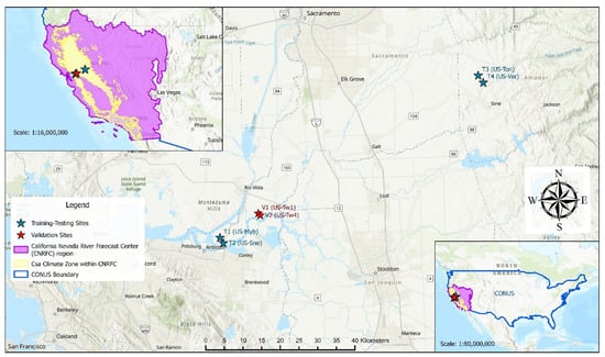
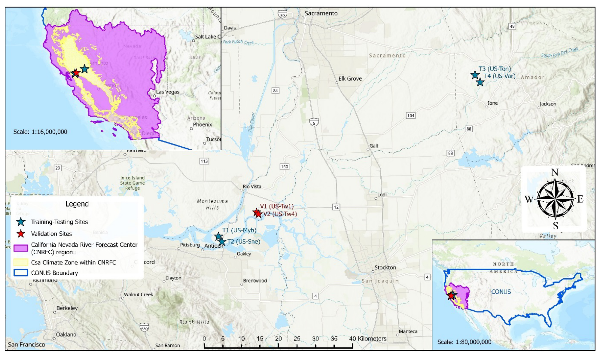
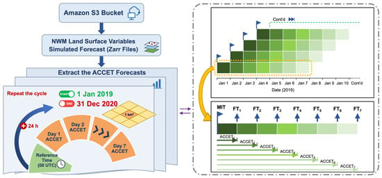
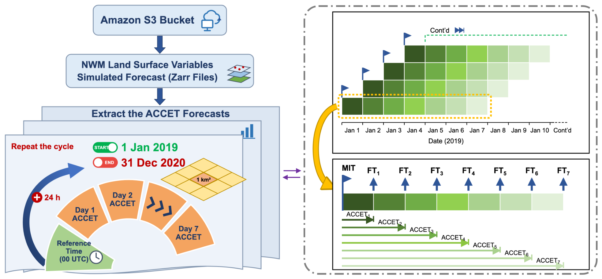
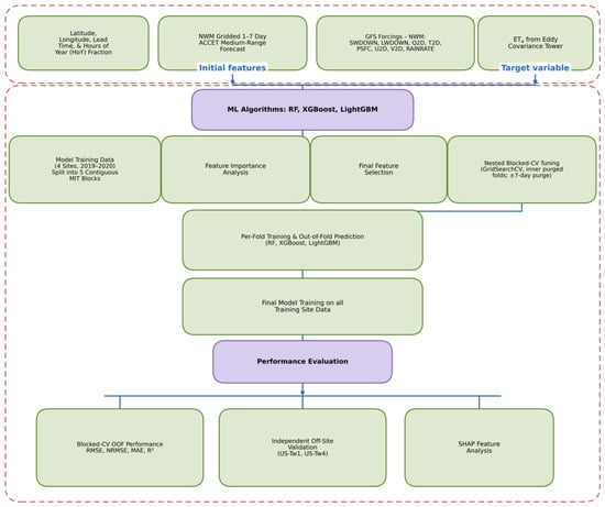
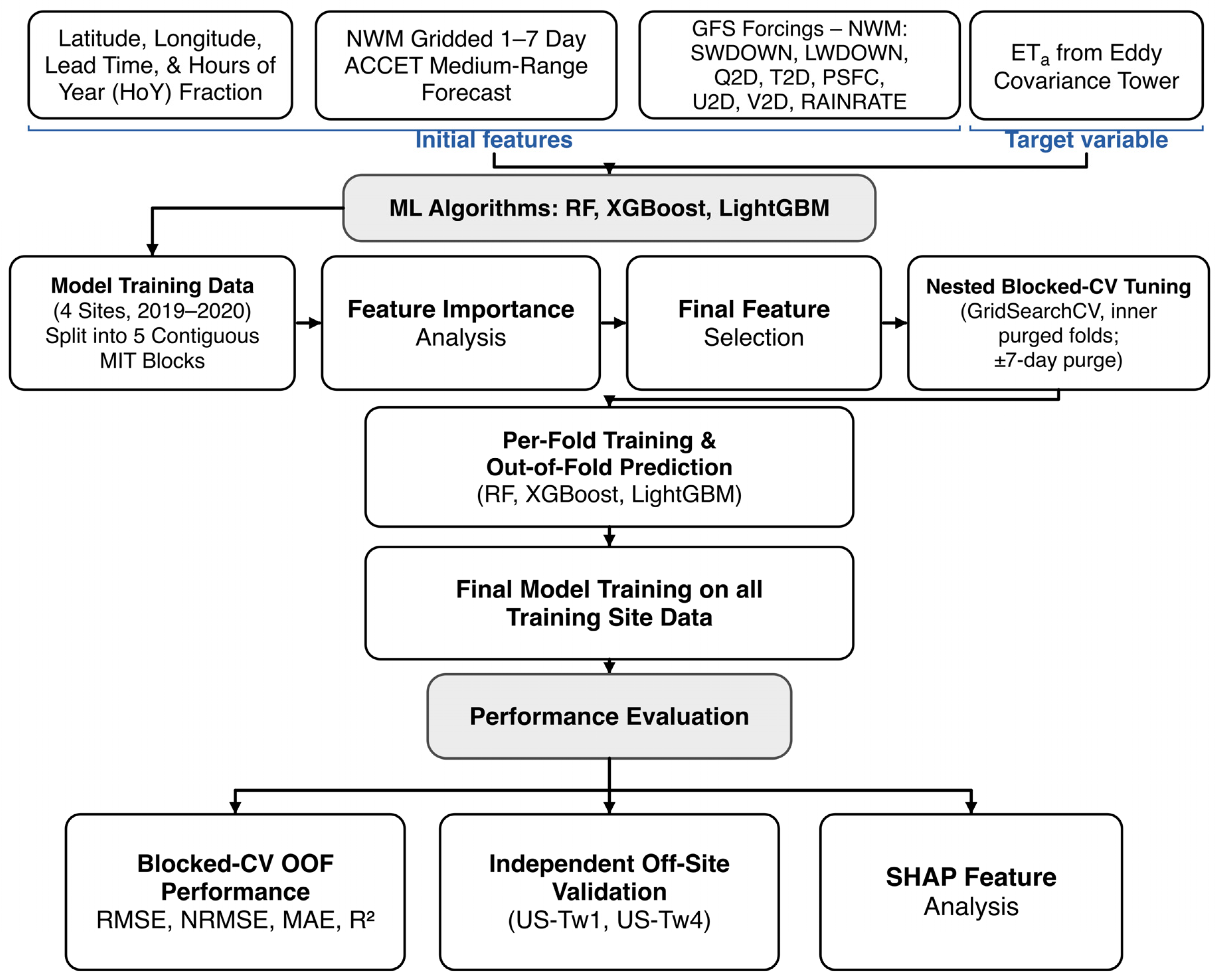
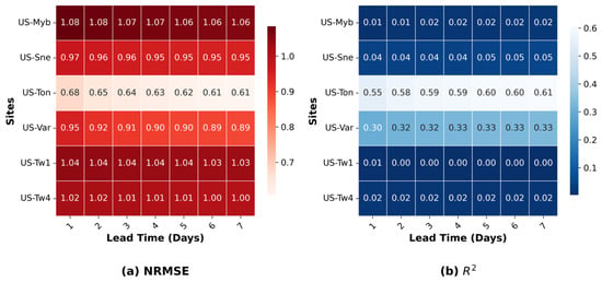
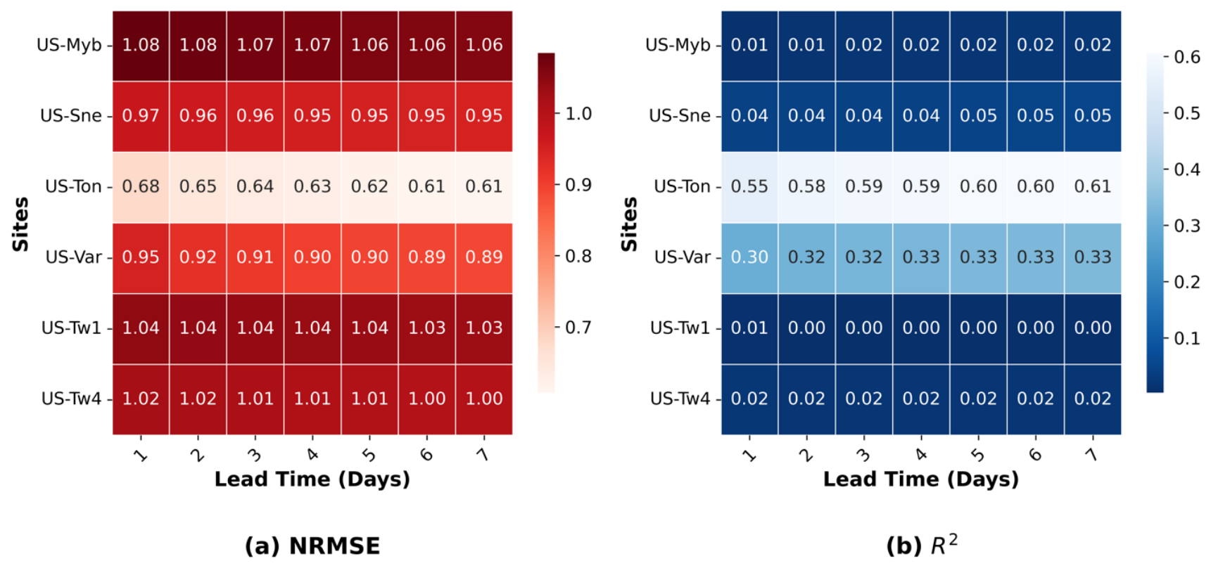
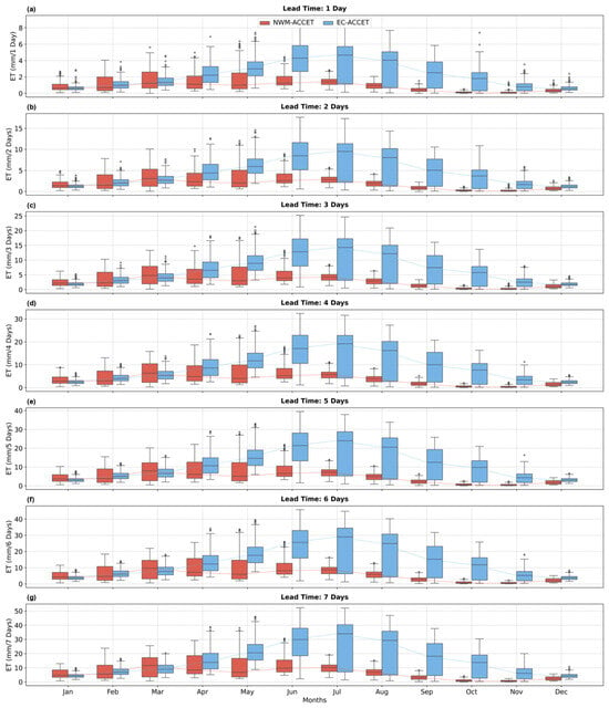
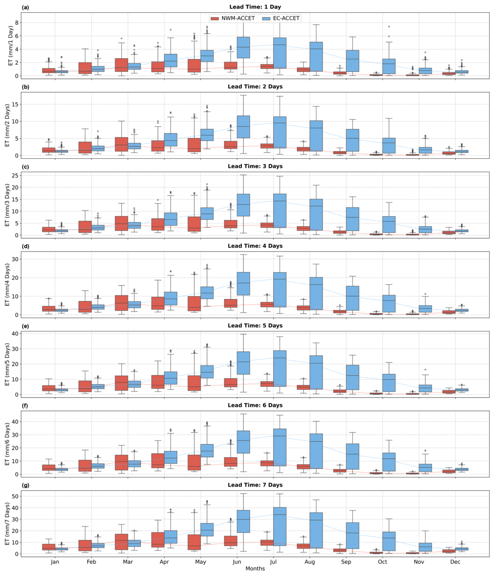
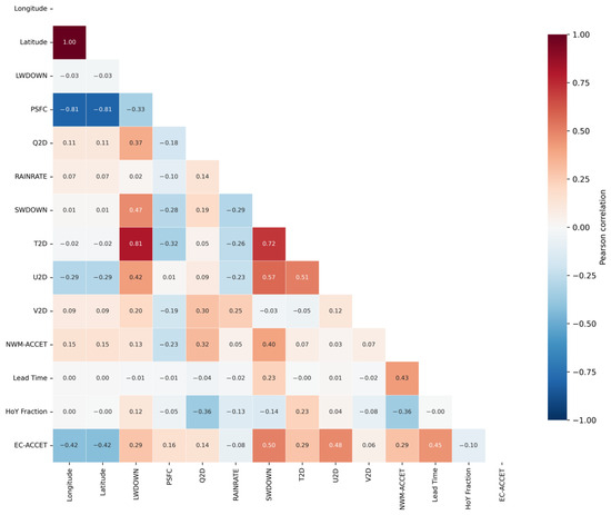
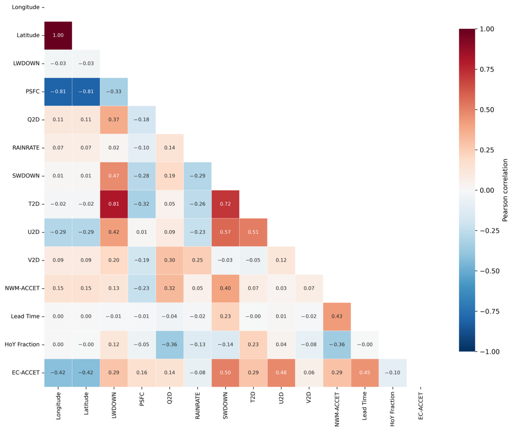
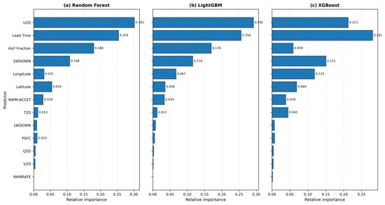
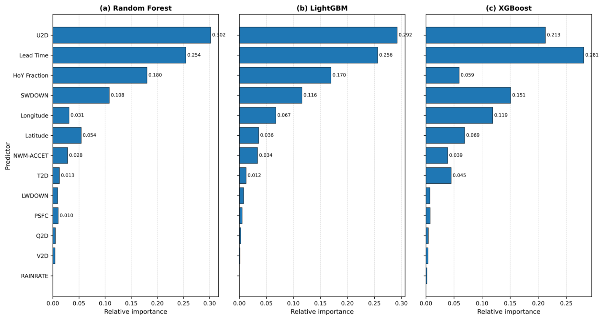
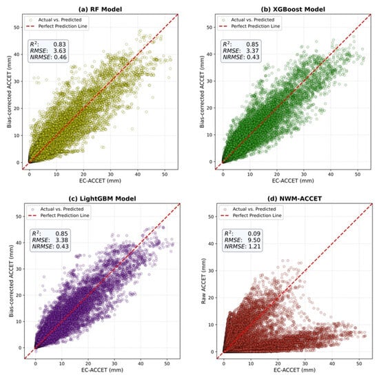
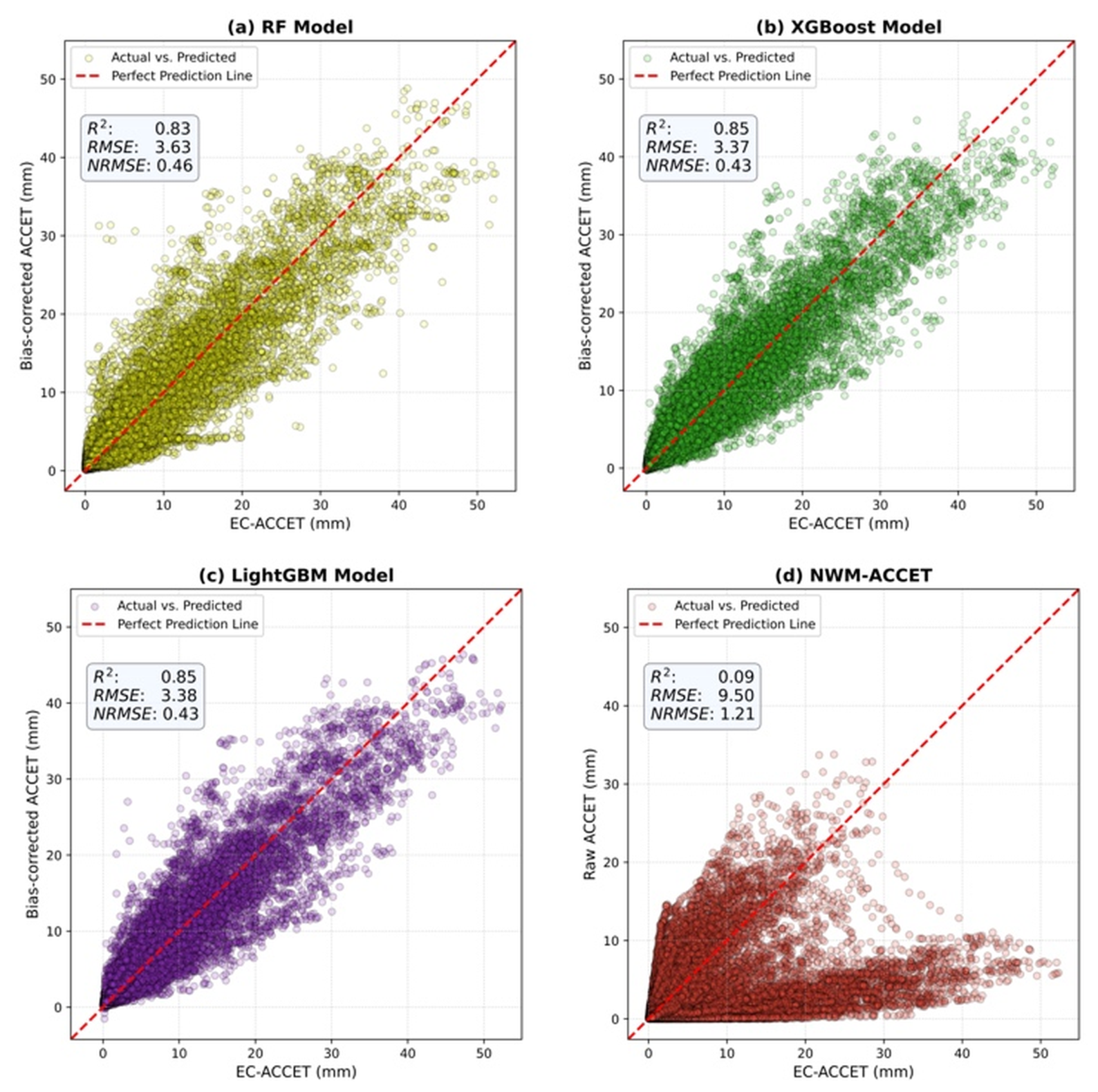
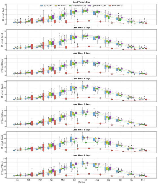
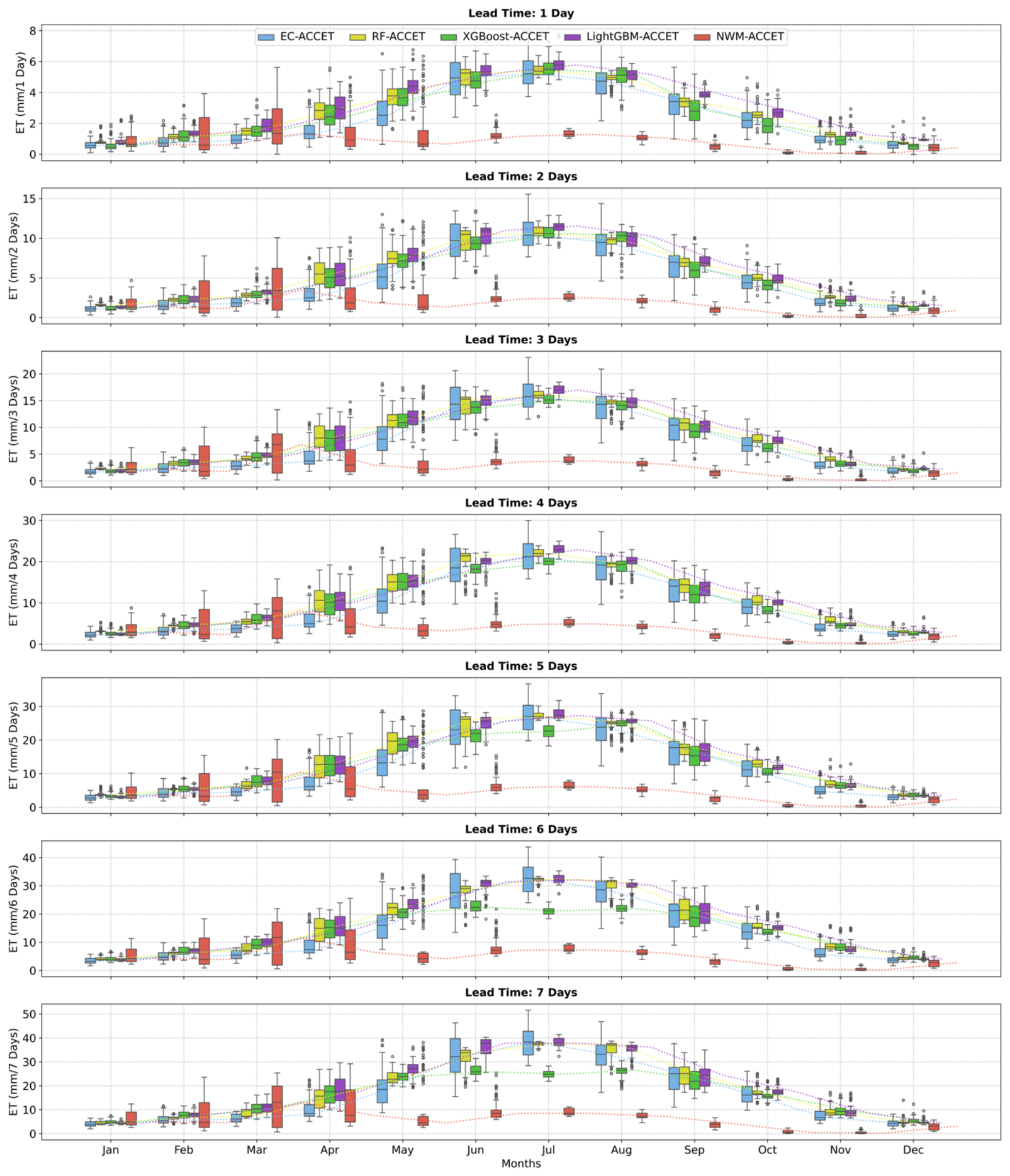
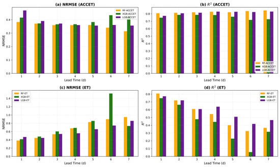
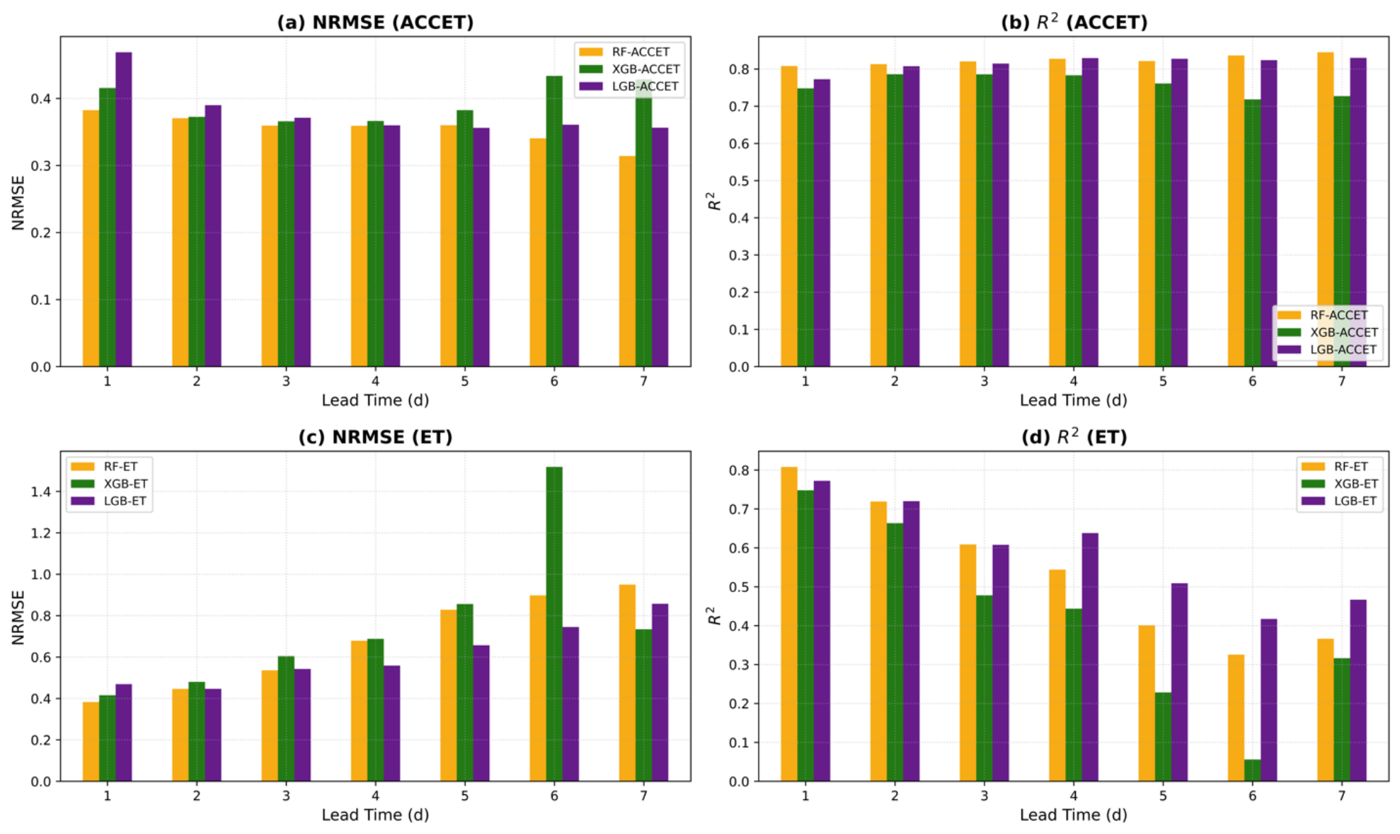
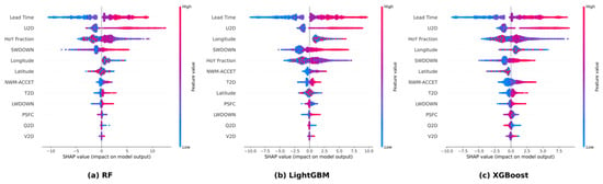
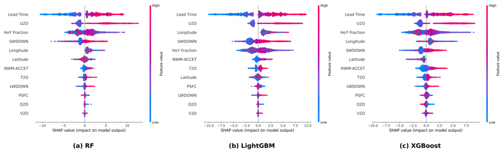

Disclaimer/Publisher’s Note: The statements, opinions and data contained in all publications are solely those of the individual author(s) and contributor(s) and not of MDPI and/or the editor(s). MDPI and/or the editor(s) disclaim responsibility for any injury to people or property resulting from any ideas, methods, instructions or products referred to in the content. |
© 2026 by the authors. Licensee MDPI, Basel, Switzerland. This article is an open access article distributed under the terms and conditions of the Creative Commons Attribution (CC BY) license.