Experimental and Numerical Study of Flow over the Weir–Flume Combination Facility

Abstract

The weir–flume combination facility is a type of river flow-measurement structure consisting of a flow weir and a Crump weir, designed to integrate flow measurement and upstream backwater regulation, while incorporating a central flume intended to provide a potential passage for aquatic organisms. This study proposes a novel combined weir–flume structure and systematically validates its hydraulic performance through integrated physical experimentation and high-fidelity numerical simulation. Laboratory tests across a flow range of 5–79 L/s revealed longitudinal water surface profiles and Froude number (Fr) distributions. The study findings show that: (1) As the flow increases, the flow regime of the combination facility transitions from flume flow to weir flow, with the critical transition point at a relative water depth of 0.885. (2) The RNG k-ε turbulence model in Flow-3D software (v11.2, Flow Science, Inc., Santa Fe, NM, USA) effectively simulates the flow movement in the weir–flume combination facility, with water depth simulation results closely matching the measured values, and the maximum relative error not exceeding 5%. (3) The Fr and flow velocity in the weir–flume combination facility first increase and then decrease along the length, forming a large, thin water layer area downstream of the facility, where both Fr and flow velocity reach their maximum values. (4) Flow measurement formulas for flume flow and weir flow are obtained through data fitting, with relative errors between the calculated values and measured flow rates being less than 3%. The present study focuses on the hydraulic performance and flow measurement capability of the proposed facility. Although the structural configuration is intended to facilitate ecological passage, its ecological effectiveness was not evaluated and requires further investigation in future studies.

1. Introduction

Hydrological monitoring of mountain rivers is a fundamental task for sustainable water resource management, the development of flood mitigation systems, and the protection of river ecosystems. However, the unique topography and hydrological characteristics of mountain rivers pose significant challenges to flow monitoring [1,2]. Firstly, due to the influence of monsoon climates, mountain rivers exhibit pronounced seasonal flow variability: during dry seasons, discharge can drop below 0.1 m³/s, while peak flows in the rainy season may exceed 10 m³/s. This wide range of flow magnitudes makes it difficult for traditional monitoring methods to maintain accuracy. Secondly, mountain rivers typically develop in V-shaped or U-shaped valleys with step-pool and plunge pool morphologies, which alter flow patterns and further complicate flow measurement [3,4].

Currently, three principal approaches are used for discharge monitoring in mountain rivers: stage–discharge relationships, velocity-based measurements, and flow-measurement structures. The stage–discharge method is simple and economical but is highly sensitive to channel erosion and sediment deposition. During flood events, hysteresis effects frequently occur, resulting in looped rating curves and substantial measurement uncertainty. Velocity-based instruments, such as Acoustic Doppler Current Profilers (ADCPs), can achieve high accuracy but require favorable hydraulic conditions and considerable operational costs, limiting their application in remote mountainous regions. Consequently, flow-measurement structures remain one of the most practical and reliable approaches for long-term discharge monitoring [5].

Various hydraulic structures have been developed for flow measurement, including labyrinth weirs [6,7,8], piano key weirs [9,10], and Crump weirs [11,12,13]. Existing studies have primarily focused on improving discharge capacity, hydraulic efficiency, and rating equations of these structures. However, most conventional weirs create physical barriers across river channels, disrupting longitudinal connectivity and impeding fish migration [14,15,16,17,18,19]. Although numerous investigations have evaluated the hydraulic performance of individual weir types, relatively little attention has been paid to balancing hydraulic measurement requirements with ecological continuity. As environmental considerations become increasingly important in river engineering, the development of flow-measurement facilities that simultaneously satisfy hydraulic and ecological objectives has emerged as a significant research challenge.

The weir–flume combination facility represents a promising solution to this challenge. By integrating a central measuring flume with laterally arranged Crump weirs, the facility forms a hydraulically coupled system capable of operating under multiple flow regimes. The flume section preserves a migration corridor for aquatic organisms and improves ecological connectivity [18], while the weir stabilizes hydraulic conditions and enhances sediment transport capacity [19]. Unlike conventional flow-measurement structures, which are typically designed either as standalone flumes or independent Crump weirs, the proposed facility establishes a coupled hydraulic configuration in which the central flume and side weirs function cooperatively under different discharge conditions. Under low-flow conditions, the central flume dominates the discharge measurement and maintains stable flow control. As discharge increases and exceeds the identified threshold, overflow is progressively activated along the Crump weirs, allowing a gradual transition from flume-controlled to weir-assisted flow conveyance. This staged hydraulic response is fundamentally different from existing single-regime structures and enables a wider operational discharge range while maintaining measurement stability. Despite these advantages, existing research on such combined structures remains limited. Most previous studies have concentrated on either flumes or weirs individually, whereas the hydraulic interaction between the two components has received insufficient investigation. In particular, several key issues remain unresolved: (i) the transition mechanism between different flow regimes has not been clearly identified; (ii) discharge measurement models applicable to a wide range of flow conditions are lacking; and (iii) the three-dimensional hydraulic characteristics governing local flow structure and downstream hydraulic transitions remain poorly understood. These knowledge gaps restrict the practical application and optimization of weir–flume combination facilities in mountain rivers.

Recent advances in computational fluid dynamics (CFD) have provided powerful tools for investigating complex hydraulic phenomena. Among available CFD platforms, Flow-3D has been widely adopted due to its TruVOF free-surface tracking algorithm and robust capability for simulating highly turbulent free-surface flows, with reported simulation errors often below 2% [20,21,22,23,24,25,26]. Previous studies have successfully applied Flow-3D to analyze hydraulic behaviors in weirs, fishways, and other hydraulic structures. Nevertheless, CFD-based investigations of integrated weir–flume systems remain scarce, particularly regarding flow-regime transitions, discharge measurement mechanisms, and three-dimensional flow structures under varying hydraulic conditions.

Therefore, the necessity of the present study arises from the lack of systematic understanding of the hydraulic behavior and discharge measurement mechanisms of weir–flume combination facilities under wide-ranging flow conditions. Unlike previous studies that focused on individual hydraulic structures, this study investigates the coupled hydraulic performance of an integrated weir–flume system through physical model experiments and numerical simulations. The main contributions of this work are as follows: (1) A relative water-depth criterion is proposed to identify the threshold of flow-regime transition within the weir–flume combination facility. (2) Segmented discharge equations are established for flume flow and weir–flume overflow conditions, improving measurement accuracy across a broad discharge range. (3) The three-dimensional distributions of water surface elevation, Froude number, and velocity field are revealed, providing insights into the hydraulic mechanisms governing flow measurement and local scour development. The findings contribute to both the theoretical understanding and practical design of environmentally compatible flow-measurement facilities for mountain rivers characterized by substantial discharge variability.

2. Materials and Methods

2.1. Experiment Method

2.1.1. Experimental Setup

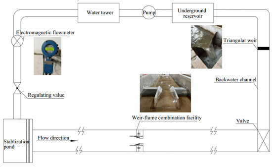
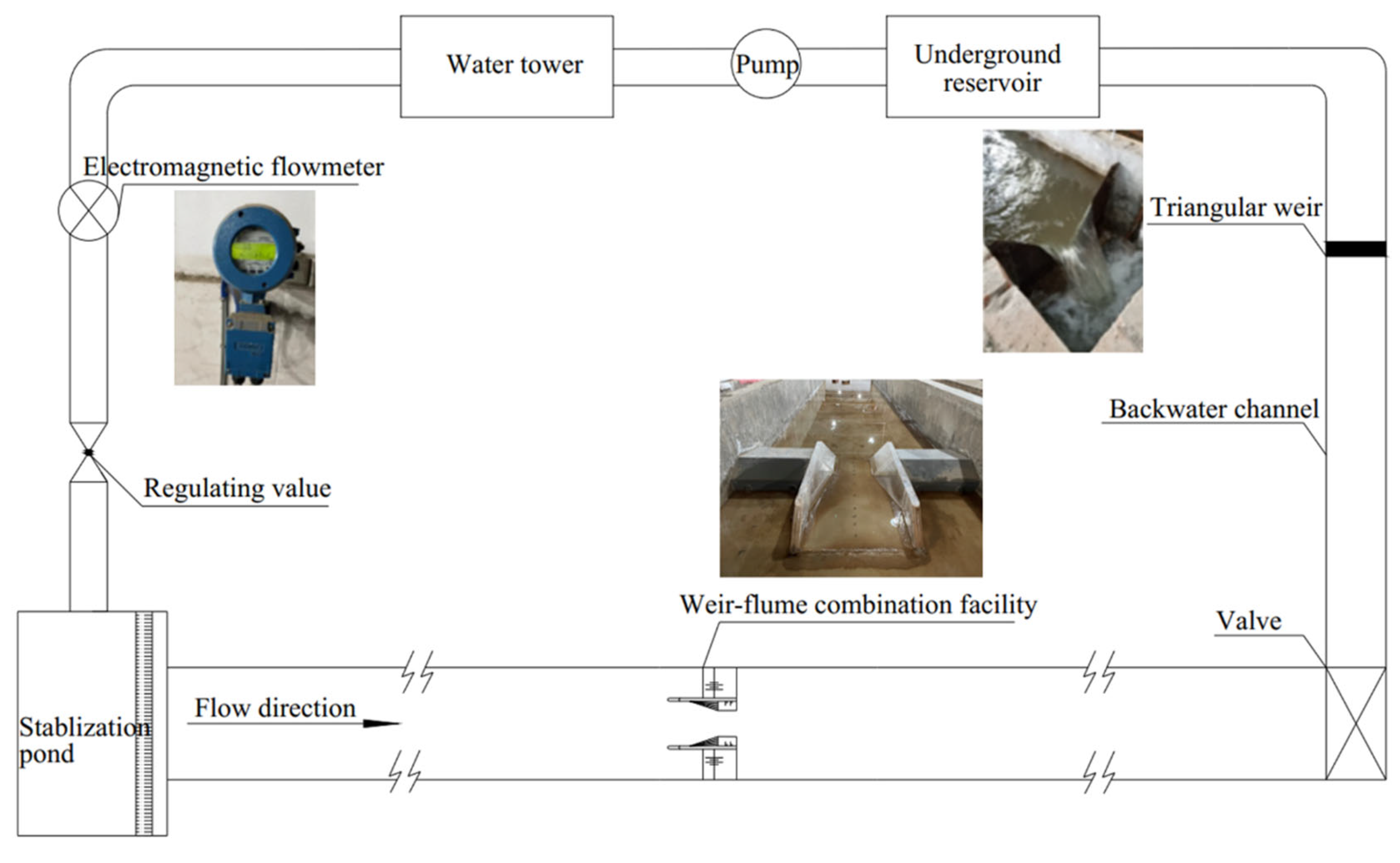
The experiments were conducted in the hydraulic and sediment laboratory of Northwest A&F University using an integrated experimental system. The system consisted of an underground reservoir, water pump, water tower, water supply pipeline, electromagnetic flowmeter, regulating valve, stabilization pond, rectangular channel, weir–flume combination facility, valve, triangular weir, and a backwater channel, as illustrated in Figure 1. The recirculating flume measured 14 m long, 1.5 m wide, and 0.5 m deep, with a smooth cement surface. Screens installed in the stabilization pond ensured the generation of smooth and uniform inlet flow conditions. Flow rate was precisely controlled through regulating valves and measured using both an electromagnetic flowmeter and a triangular weir, achieving an accuracy of ±1%. Water depth measurements were obtained using a water level probe with a precision of ±0.1 mm. The average flow velocity at each measurement point was determined using a portable screw current meter (LS300-A, Weifang Jinshui Huayu Information Technology Co., Ltd., Weifang, China), which has a measurement error of ±1.5% and was operated with a sampling time of 60 s.

Figure 1. Experiment system layout.

2.1.2. Body Shape Parameter and Experiment Arrangement

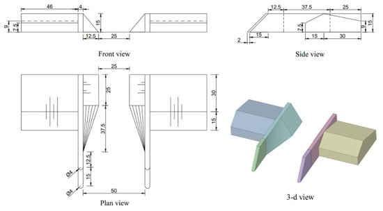
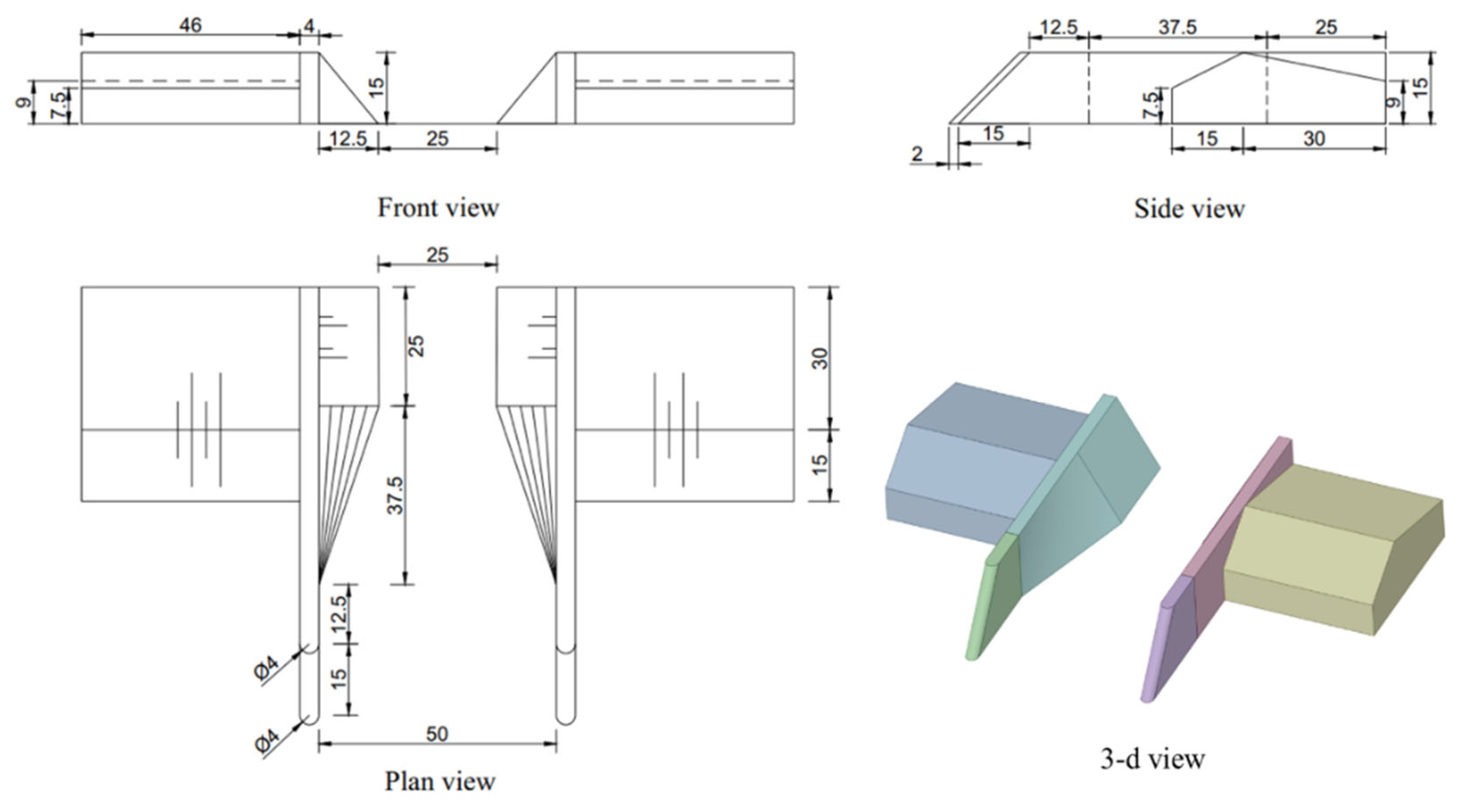
The weir–flume combination facility consists of a Crump weir and a sluicing flume. The Crump weir has a 1:2 slope on the water-facing side and a 1:5 slope on the back-water side, ensuring a smooth water surface transition [12]. Constructed from polyvinyl chloride board, the weir has a height (P) of 15 cm, a length of 45 cm, and a width of 46 cm. The sluicing flume comprises four sections: a water diversion section, a rectangular section, a contraction transition torsion section, and a trapezoidal section. It was fabricated from organic glass. The water diversion section features a semi-cylindrical partition wall with a 45° slope toward the water surface and a thickness of 4 cm. Previous studies indicate that this 45° partition wall design effectively enhances water diversion and sediment discharge [18]. The sluicing flume has a flat bottom, with the trapezoidal section’s bottom width (b) measuring 25 cm. The entire facility matches the channel width of 1.5 m. Additional dimensional details are provided in Figure 2.

Figure 2. Weir–flume combination facility body shape parameter diagram (unit: cm).

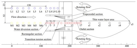
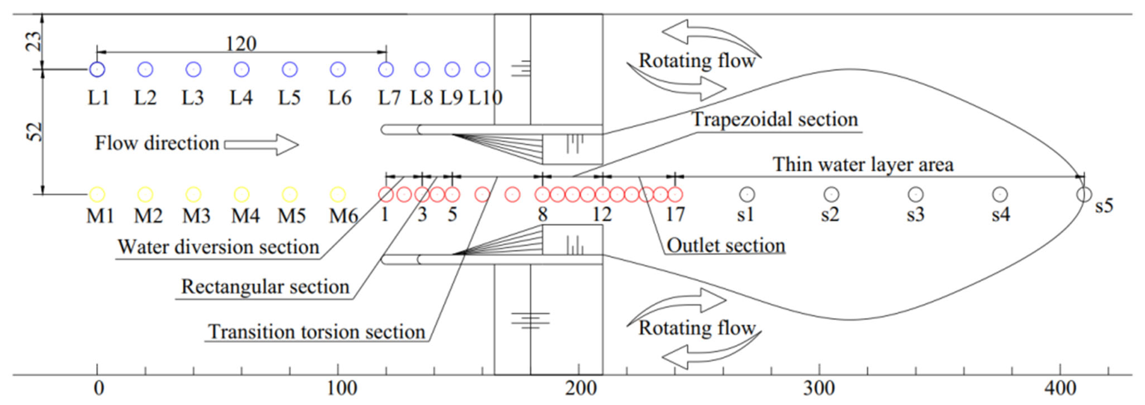
The experiment investigated 17 flow conditions with discharge rates ranging from 5 to 79 L/s. Based on the flow characteristics and facility geometry, water level measurement points were divided into four areas: 26 points (M1–M6 and L1–L10) in the upstream section, 5 points (S1–S5) in the thin water layer downstream of the facility, 12 points (1–12) within the sluicing flume, and 5 points (13–17) near the outlet. The measurement point arrangement is shown in Figure 3, while the control sections in the sluicing flume are detailed in Table 1. For each flow condition, after achieving flow stability and recording water levels, velocity distributions along the flume’s central axis were measured using a portable screw current meter (LS300-A) to determine vertical average velocities. All tests were conducted under free outflow conditions.

Figure 3. Layout of measurement points of the weir–flume combination facility (unit: cm).

Table 1. Control the section position in the sluicing flume.

Section Number	Distance from Section M1/cm	Section Number	Distance from Section M1/cm
1	120	10	197.5
2	127.5	11	203.75
3	135	12	210
4	141.25	13	215
5	147.5	14	220
6	160	15	225
7	172.5	16	230
8	185	17	235
9	191.25	-	-

2.1.3. Dimensional Analysis

The hydraulic performance of the proposed weir–flume combination facility is primarily governed by the discharge Q, gravitational acceleration g, upstream water depth h, characteristic structural dimensions (such as the flume wall height d and weir height p), flow velocity V, and fluid properties. According to the Buckingham π theorem, the hydraulic behavior of the structure can be expressed using several dimensionless parameters, including the Froude number:

$${\mathrm{F}}_r={\displaystyle \frac{V}{\sqrt{gh}}}$$

(1)

the relative water depth:

$${\displaystyle \frac{h_4}{\sqrt{d}}}$$

(2)

and the relative upstream head:

$${\displaystyle \frac{h_w}{h_w+p}}$$

(3)

Because the present experiments were conducted under fully turbulent open-channel flow conditions, viscous effects are relatively small compared with gravitational effects. Therefore, the Froude number is considered the dominant similarity criterion. Based on this dimensional analysis, the relative water depth (h₄/d) was selected to identify the transition between flume flow and weir flow, while (h_w/(h_w + p)) was adopted to characterize the hydraulic behavior after overtopping.

2.2. Measurement Uncertainty Analysis

To ensure the reliability of the experimental data, the uncertainties associated with water depth, discharge, and flow velocity measurements were evaluated according to the specifications of the measuring instruments and repeated measurements. Water depth was measured using a point gauge with a resolution of 0.1 mm, resulting in a relative uncertainty generally below 0.5% under the experimental water depths. Discharge was monitored using an electromagnetic flowmeter (Model Proline Promag P 300, Endress+Hauser Flowtec AG, Reinach, Switzerland) with an accuracy of ±0.5% of the measured value, and the flow rate was simultaneously checked using a calibrated triangular weir to ensure measurement consistency. Flow velocity was measured using an LS300-A portable current meter with an accuracy of ±1% of the measured value. At each measuring section, velocity measurements were repeated three times after the flow became stable, and the average value was adopted for subsequent analyses.

Because the hydraulic parameters investigated in this study, including the water surface profile, Froude number, flow threshold, and discharge equations, were derived from averaged measurements rather than individual observations, the random measurement errors were substantially reduced. The remaining uncertainties were considerably smaller than the observed hydraulic variations among different flow conditions and therefore did not affect the identification of flow regimes, the determination of the flow threshold, or the fitting accuracy of the discharge equations.

2.3. Consideration of Scale Effects

The experiments were conducted under laboratory-scale conditions; therefore, potential scale effects were evaluated using dimensional analysis. For open-channel free-surface flows such as those investigated in this study, the dominant similarity criterion is the Froude number (Fr), which ensures dynamic similarity of gravity-controlled flows. The experimental design maintained Froude similarity as the governing scaling principle.

The Reynolds number (Re) in all experimental cases exceeded the commonly accepted threshold for fully turbulent open-channel flow, indicating that viscous effects are negligible and that the flow regime is dynamically similar to prototype mountain rivers. Although minor scale effects related to surface tension (Weber number) and wall roughness may still exist in laboratory flumes, their influence on the stage–discharge relationship is limited under fully turbulent conditions. Therefore, the derived hydraulic relationships and flow-measurement equations are expected to remain applicable at prototype scale after appropriate field calibration.

2.4. Numerical Method

In this study, the FLOW-3D numerical model was employed to simulate the flow characteristics, as it is particularly suitable for solving complex fluid dynamics problems and modeling unsteady three-dimensional free surface flows with intricate geometries. The model utilizes the TruVOF method to accurately track free surface variations by exclusively computing liquid cells while neglecting gas cells. Additionally, the Fractional Area-Volume Obstacle Representation (FAVOR) technique was implemented to effectively simulate domain boundaries, including any obstacles present in the flow field [27].

2.4.1. Governing Equations

The water is Newtonian fluid. Therefore, the flow field could be described by the continuity equation (Equation (4)) and the RANS (Reynolds averaged Navier–Stokes) equation (Equation (5)) [28]. The water is treated as an incompressible Newtonian fluid with constant density, which is a standard assumption for open-channel hydraulic simulations.

$${\displaystyle \frac{\mathsf{\partial }p}{\mathsf{\partial }t}}+{\displaystyle \frac{\mathsf{\partial }{u}_i}{\mathsf{\partial }{x}_i}}=0$$

(4)

$${\displaystyle \frac{\partial (\rho {\mathrm{u}}_{\mathrm{i}})}{\partial \mathrm{t}}}+{\displaystyle \frac{\partial (\rho {\mathrm{u}}_{\mathrm{i}}{\mathrm{u}}_{\mathrm{j}})}{\partial {\mathrm{x}}_{\mathrm{j}}}}=-{\displaystyle \frac{\partial \mathrm{p}}{\partial {\mathrm{x}}_{\mathrm{i}}}}+{\displaystyle \frac{\partial }{\partial {\mathrm{x}}_{\mathrm{j}}}}\left(\mu {\displaystyle \frac{\partial {\mathrm{u}}_{\mathrm{i}}}{\partial {\mathrm{x}}_{\mathrm{j}}}}-\rho \overline{{\mathrm{u}}_{\mathrm{i}}^{\prime }{\mathrm{u}}_{\mathrm{j}}^{\prime }}\right)+{\mathrm{S}}_{\mathrm{i}}$$

(5)

where $\mathsf{\rho }$ is the density of the water, $\mathrm{kg}/{\mathrm{m}}^3$; t is the time, s; u_i and u_j are the average velocity (i = 1, 2, 3; j = 1, 2, 3), u₁, u₂, u₃ represents average velocity components in Cartesian coordinates x, y, and z respectively, m/s; $\mathsf{\mu }$ is the dynamic viscosity of the fluid, N∙s/m²; p is the pressure of the fluid, N/m²; and Si is body force, S₁ = 0, S₂ = 0, S₃ = $-\mathsf{\rho }\mathrm{g}$, N.

2.4.2. Turbulence Model

The RNG k-ε turbulence model provided by Flow-3D software was used to simulate the turbulence in the water flow. The RNG k-ε model was selected because the flow within the proposed weir–flume combination facility involves strong streamline curvature, local flow separation, recirculation, rapid acceleration, and free-surface turbulence. Compared with the standard k-ε model, the RNG k-ε model introduces an additional term in the turbulent dissipation equation, improving its capability to predict rapidly strained and highly curved flows. Previous studies have also demonstrated that the RNG k-ε model provides reliable predictions for hydraulic structures such as weirs, flumes, and open-channel flows. Therefore, it was considered an appropriate compromise between computational efficiency and simulation accuracy for the present study. Moreover, the suitability of the selected turbulence model was verified through comparison between simulated and measured water-surface profiles, with maximum relative errors below 5%.

The RNG k-ε model is an improvement of the standard k-ε model (Equations (6)–(10)), which reflects small-scale effects by large-scale motion and modified viscosity terms and can handle the flow with a large degree of curvature well. The RNG k-ε model had a good capability for the numerical simulation of transitional flow [29,30,31].

$${\displaystyle \frac{\partial (\rho \mathrm{k})}{\partial \mathrm{t}}}+{\displaystyle \frac{\partial (\rho \mathrm{k}{\mathrm{u}}_{\mathrm{i}})}{\partial {\mathrm{x}}_{\mathrm{i}}}}={\displaystyle \frac{\partial }{\partial {\mathrm{x}}_{\mathrm{j}}}}\left[{\alpha }_{\mathrm{k}}{\mathsf{\mu }}_{\mathrm{eff}}{\displaystyle \frac{\partial \mathrm{k}}{\partial {\mathrm{x}}_{\mathrm{j}}}}\right]+{\mathrm{G}}_{\mathrm{k}}+\rho \mathsf{\epsilon }$$

(6)

$${\displaystyle \frac{\partial (\rho \mathsf{\epsilon })}{\partial \mathrm{t}}}+{\displaystyle \frac{\partial (\rho \mathsf{\epsilon }{\mathrm{u}}_{\mathrm{i}})}{\partial {\mathrm{x}}_{\mathrm{i}}}}={\displaystyle \frac{\partial }{\partial {\mathrm{x}}_{\mathrm{j}}}}\left[{\alpha }_{\mathsf{\epsilon }}{\mathsf{\mu }}_{\mathrm{eff}}{\displaystyle \frac{\partial \mathrm{k}}{\partial {\mathrm{x}}_{\mathrm{j}}}}\right]+{\displaystyle \frac{{\mathrm{C}}_{1\mathsf{\epsilon }}^{\ast }\mathsf{\epsilon }}{\mathrm{k}}}{\mathrm{G}}_{\mathrm{k}}-{ \mathrm{C}}_{2\mathsf{\epsilon }}\rho {\displaystyle \frac{{\mathsf{\epsilon }}^2}{\mathrm{k}}}$$

(7)

$${\mathrm{C}}_{1\mathsf{\epsilon }}^{\ast }={\mathrm{C}}_{1\mathsf{\epsilon }} - {\displaystyle \frac{\mathsf{\eta }(1 - \mathsf{\eta }/{\mathsf{\eta }}_0)}{1+\mathsf{\beta }{\mathsf{\eta }}^3}}$$

(8)

$$\mathsf{\eta }={(2{\mathrm{E}}_{\mathrm{ij}}·{\mathrm{E}}_{\mathrm{ij}})}^{1/2}{\displaystyle \frac{\mathrm{k}}{\mathsf{\epsilon }}}$$

(9)

$${\mathrm{E}}_{\mathrm{ij}}={\displaystyle \frac{1}{2}}\left({\displaystyle \frac{\partial {\mathrm{u}}_{\mathrm{i}}}{\partial {\mathrm{x}}_{\mathrm{j}}}}+{\displaystyle \frac{\partial {\mathrm{u}}_{\mathrm{j}}}{\partial {\mathrm{x}}_{\mathrm{i}}}}\right)$$

(10)

where k is turbulence kinetic energy, m²/s²; ε is turbulence dissipation rate, kg·m²/s³; x_i, x_j is the axis in Cartesian coordinates (i = 1, 2, 3; j = 1, 2, 3), x₁, x₂ and x₃ represent Cartesian coordinates x, y, and z, respectively; ${\mathsf{\mu }}_{\mathrm{eff}} = \mathsf{\mu } + {\mathsf{\mu }}_{\mathrm{t}}$, ${\mathsf{\mu }}_{\mathrm{t}}$ is the turbulent viscosity of fluid, N∙s/m²; and G_k is the turbulent energy caused by the average velocity gradient. In this paper, ${\mathsf{\alpha }}_{\mathrm{k}}$ and ${\mathsf{\alpha }}_{\mathsf{\epsilon }}$ were set as 1.39, C_1ε was set as 1.42, C_2ε was set as 1.68, ${\mathsf{\eta }}_0$ was set as 4.377, and $\mathsf{\beta }$ was set as 0.012.

2.4.3. Model Establishment and Mesh Generation

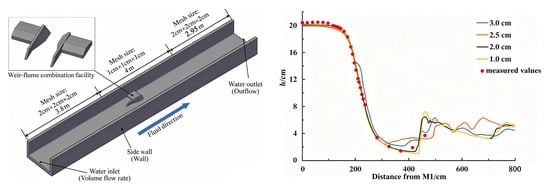
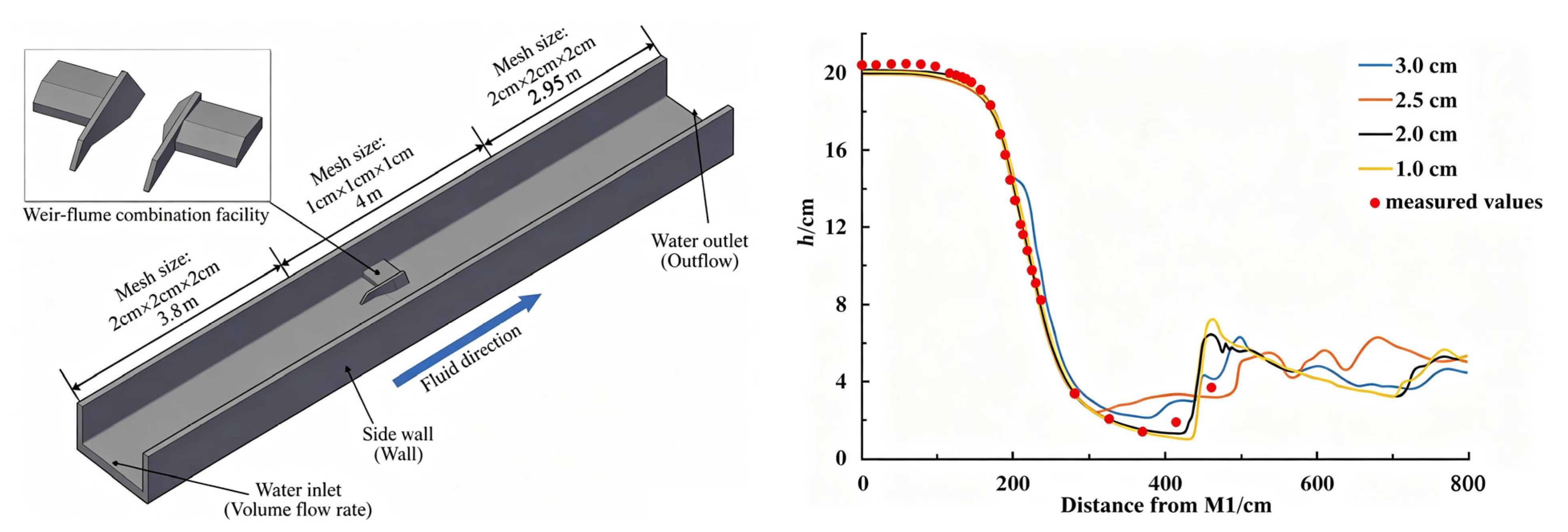
The structured Cartesian mesh was employed to balance computational efficiency and solution accuracy. Grid independence was evaluated using four mesh sizes (3, 2.5, 2, and 1 cm). As shown in Figure 4, the predicted longitudinal water-surface profiles became nearly identical when the mesh size was refined from 2 cm to 1 cm, indicating mesh-independent solutions. Therefore, a base mesh size of 2 cm × 2 cm × 2 cm was adopted. Considering the large hydraulic gradients in the downstream thin-water-layer region and the local scour area, local mesh refinement was applied within 4 m downstream of the weir using a grid size of 1 cm × 1 cm × 1 cm. The final computational domain contained approximately 3.22 million cells, providing sufficient resolution for both global flow characteristics and local hydraulic phenomena.

Figure 4. Model setup and schematic of the weir–flume combination facility (M1 denotes the upstream reference measurement point).

The local oscillations observed in the downstream water surface profiles (approximately 300–800 cm from M1) are primarily associated with the highly turbulent free-surface flow downstream of the weir–flume combination facility, where flow separation, recirculation, and hydraulic-jump-like phenomena occur. These oscillations reflect the complex hydraulic behavior in the thin-water-layer region rather than numerical instability, as demonstrated by the convergence of the solutions obtained using the 2 cm and 1 cm grids. Moreover, the purpose of the grid independence test is to evaluate solution convergence rather than to eliminate local hydraulic fluctuations. Therefore, the slight oscillations observed in the downstream region do not affect the selection of the optimal mesh size or the reliability of the numerical simulations.

2.4.4. Calculation Method and Boundary Conditions

To ensure consistency between the numerical simulation and the laboratory experiments, the computational boundaries were specified according to the experimental hydraulic conditions. The upstream boundary was prescribed as a volume flow rate inlet, with the discharge corresponding to the measured value for each experimental case. The downstream boundary was defined as an outflow boundary, allowing water to leave the computational domain without imposing an artificial tailwater condition. The channel bed and sidewalls were treated as no-slip wall boundaries, whereas the top boundary was assigned as an atmospheric pressure boundary to allow free-surface evolution. These boundary settings reproduced the open-channel hydraulic conditions of the physical model while minimizing artificial numerical effects at the computational boundaries. The boundary configuration is shown in Figure 4.

3. Results

3.1. Experiment Results and Analysis

3.1.1. Overcurrent Forms and Hydraulic Characteristics

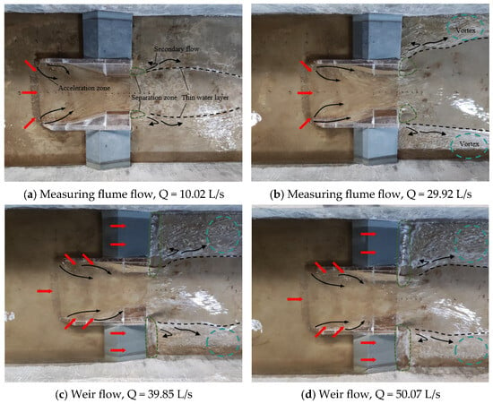
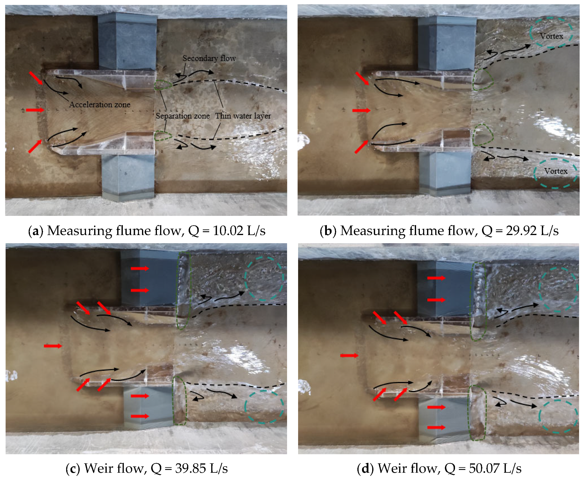
The discharge range of seasonal rivers is greatly affected by rainfall. When the flow rate is low, the water can pass through the main channel, but when the flow rate is high, the overall water flow will overflow from the main channel to the riverbank. The weir–flume combination facility is similar to seasonal rivers. Figure 5 shows two overcurrent forms of the weir–flume combination facility in different flow ranges. When the flow was small, all the water flowed through the sluicing flume, and there was no overflow on both sides of the Crump weir crest, as shown in Figure 5a. When the flow rate continued to increase and the water depth exceeded the height of the Crump weir, the water passed through the sluicing flume and the top of the weir on both sides at the same time, as shown in Figure 5b. Therefore, the critical flow between the in-flume flow and the weir flow is called the flow threshold. Since the width of the cross-section increased suddenly after the weir flow, the relationship between water depth and flow rate changed with the flow in the flume, so it is necessary to determine the flow threshold. Through experiments, it was found that when the flow rate of the weir–flume combination facility in this study was greater than 32.75 L/s, the weir crests on both sides began to flow, and the side walls of the sluicing flume overflowed. Experimental research has found that the flow threshold corresponding to the two types of overflow forms of the combined weir and trough facilities is 32.75 L/s, and the water depth h₄ at measuring point 4 in the spillway has a stable relationship with the flow rate passing through the spillway. The dimensionless relative water depth was obtained by taking the ratio h₄/d of the water depth at this point and the partition height d of the drainage volume flume, and the value corresponding to the flow threshold was called the relative water depth threshold. Five measurement points (Points 1–5) located in the inlet section of the measuring flume were initially evaluated as potential hydraulic control points. Among them, Measurement Point 4 exhibited the strongest and most stable relationship with discharge over the entire experimental range. Therefore, the relative water depth at Measurement Point 4 was selected as the flow-regime indicator. According to the results, the relative water depth threshold h₄/d = 0.885 can be used as a standard to judge the flow mode. For the water flow characteristics in the flume and the weir flow characteristics of the weir–flume combined structure, the flow field observed in the experiment exhibits complex flow features and can be divided into five distinct regions [32], as shown in Figure 5. When water enters the flume, the flow direction changes, accompanied by a certain increase in velocity. The separation zone is generated by the boundary shape and pressure gradient, and its extent expands under weir-flow conditions. A secondary flow develops downstream of the separation zone, inducing a recirculating flow. Behind the flume, influenced by inertia, a thin water layer forms, which propagates toward both sides of the channel in a manner similar to a hydraulic jump, generating turbulent disturbances and localized vortices. Similar flow patterns were observed under other experimental conditions. These flow features exhibit hydraulic-jump-like characteristics associated with rapid flow expansion and intense turbulence, rather than a fully developed hydraulic jump.

Figure 5. Flow patterns and characteristics of combined weir and flume facilities.

3.1.2. Flow State Discrimination and Water Surface Profile

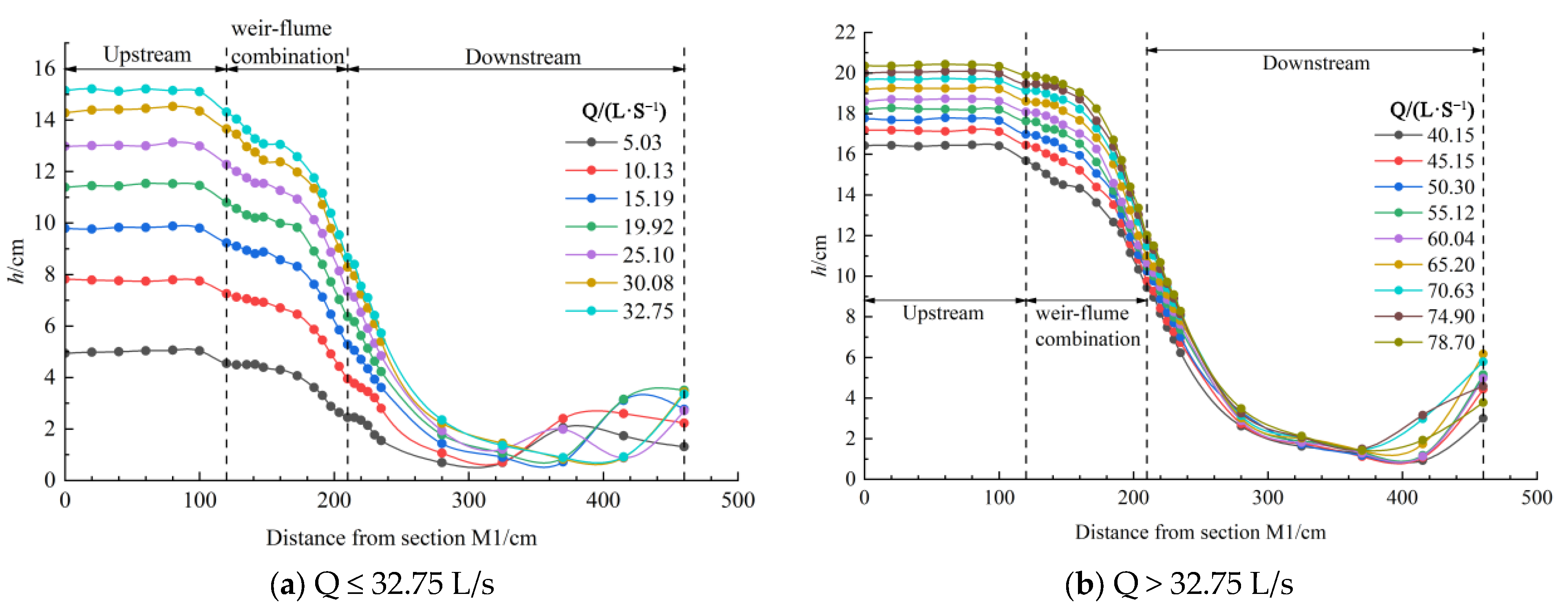
As shown in Figure 6, the upstream water surface before the inlet of the weir–flume combination is relatively stable for all discharges. In this region, the water depth changes only slightly along the channel, indicating a gradually varied subcritical flow controlled by the downstream hydraulic control. For Q ≤ 32.75 L/s, the upstream centerline depth increases from approximately 5.0 cm to 15.2 cm as the discharge increases. For Q > 32.75 L/s, the upstream depth increases from approximately 16.4 cm to 20.3 cm. Although the discharge almost doubles in the high-flow group, the upstream depth increases by only about 4 cm, indicating that the weir–flume combination acts as a hydraulic control and limits the upstream water-level response. After the flow enters the weir–flume combination, the water surface begins to decline. In the rectangular inlet section, the decrease is relatively small because the rounded 45° transition of the partition wall reduces abrupt separation and allows the streamlines to adjust gradually. However, in the torsional and trapezoidal contraction sections, the cross-sectional area decreases more rapidly. According to the continuity equation, the local velocity must increase as the available flow area decreases. Consequently, part of the pressure head is converted into velocity head, and the water surface drops sharply.

Figure 6. Changes in water surface profile along the middle vertical plane.

The different downstream profiles in Figure 6a,b indicate two flow patterns separated by the discharge threshold of approximately 32.75 L/s. When Q ≤ 32.75 L/s, the jet momentum is relatively weak. The flow expands after leaving the flume, and separated shear layers and local recirculation zones develop on both sides of the downstream region. Therefore, the water depth distribution in the thin-layer region is not strictly monotonic with discharge. Some curves intersect or fluctuate between approximately x = 320 cm and x = 430 cm, which is caused by the different positions of the local surface roller and weak hydraulic jump under different discharges. When Q > 32.75 L/s, the jet momentum becomes stronger and the supercritical thin layer extends farther downstream. The downstream recovery is more evident near the tail region, especially after x ≈ 400 cm, where the water depth rises again because of tailwater influence and hydraulic-jump-induced energy dissipation.

3.1.3. Location of Critical Water Depth Profile

The calculation of the Froude number (Fr) on the section of each measurement point can more accurately identify the flow state and determine the location of slow flow, critical flow, and rapids. Thus, it provides a theoretical basis for selecting water level measurement points of the facility. There are two different flow modes in the weir–flume combination facility, so two different calculation modes are selected. When the flow rate does not exceed the flow threshold, the flow area is used to calculate Fr (Equation (11)). When the flow rate exceeds the flow threshold, the Crump weir on both sides begins to overflow, and the area of overflow is difficult to determine. Therefore, a portable current meter is used to measure the vertical flow rate distribution, and the average flow velocity on the vertical line of the measurement point is used to calculate Fr (Equation (12)).

$$\mathrm{F} ={\displaystyle \frac{\stackrel{\mathrm{-}}{\mathrm{v}}}{\sqrt{\mathrm{g}\stackrel{\mathrm{-}}{\mathrm{h}}}}}={\displaystyle \frac{\mathrm{Q}}{\mathrm{A}\sqrt{\mathrm{g}\stackrel{\mathrm{-}}{\mathrm{h}}}}}$$

(11)

$$\mathrm{Fr} ={\displaystyle \frac{{\stackrel{\mathrm{-}}{\mathrm{v}}}_{\mathrm{ver}}}{\sqrt{\mathrm{gh}}}}$$

(12)

where, $\stackrel{\mathrm{-}}{\mathrm{v}}$ is the average velocity of the section (m/s); g is the acceleration of gravity (9.81 m/s²); Q is the overcurrent flow (m³/s); $\stackrel{\mathrm{-}}{\mathrm{h}}$ is the average depth of the section (m); A is the area of flow (m²); ${\stackrel{\mathrm{-}}{\mathrm{v}}}_{\mathrm{ver}}$ is the average velocity on the vertical line of the measurement point (m/s); and h is the depth of the measurement point (m).

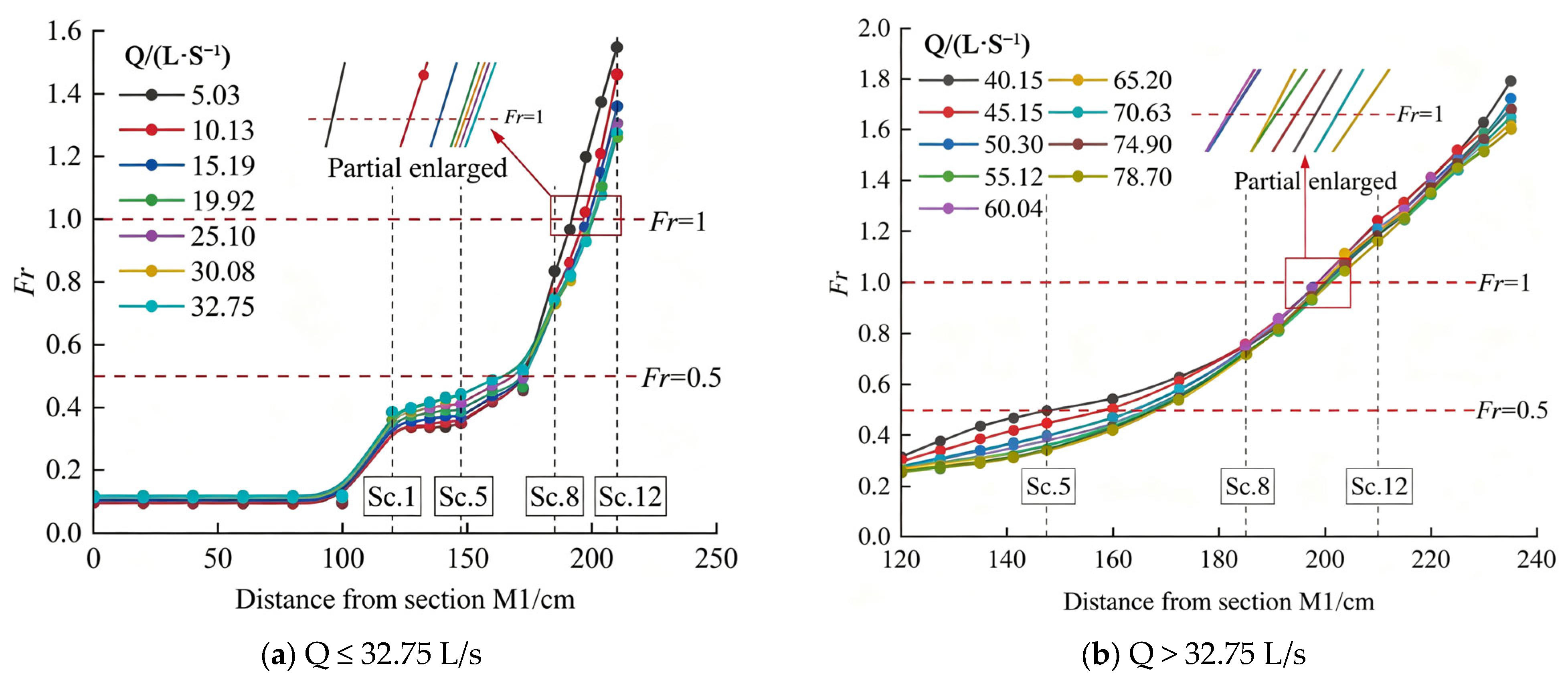
Figure 7a shows the distribution of Froude number along the threshold flow range. As can be seen from the figure, the Froude number (Fr) in the front section (0–100 cm) of the inlet of the sluicing flume has a small fluctuation, keeping at about 0.1. However, when the water is into the sluicing flume, the cross-section of the flow area suddenly decreases and the flow velocity increases rapidly, resulting in a sharp increase in the Fr from 0.1 to 0.4. In the sluicing flume, Fr increases along the way, with a large increase rate in the torsion section and trapezoidal section, while Fr increases slowly in the water diversion section and rectangular section (120–147.5 cm). According to Figure 7b, when the flow is greater than the threshold flow, the distribution of Fr in the sluicing flume is similar to that in the threshold flow, and the increase rate of Fr in the back section is greater than that in the front section of the sluicing flume.

Figure 7. Distribution of Froude number along the path under different flow rates.

According to the line of Fr = 1 in Figure 7, whether inside or outside the threshold flow, the critical depth section appears in the trapezoidal section of the sluicing flume. According to the partially enlarged detail in Figure 7, When Q ≤ 32.75 L/s, the critical depth section position gradually moves backwards with the increase of flow rate. However, when Q > 32.75 L/s, the calculated location of the critical depth section exhibits greater scatter than that observed under flume-flow conditions. This increased variability is primarily associated with the different Froude-number calculation approaches adopted for the two flow regimes rather than indicating a change in the overall hydraulic behavior. Although the exact location of the critical depth section becomes less stable under weir-flow conditions, the results consistently indicate that the critical section remains within the trapezoidal section of the measuring flume, which supports the hydraulic interpretation presented in this study. According to the selection standard of water level measurement points, the Froude number of measurement points should be less than 0.5 [6]. From the Fr = 0.5 line in Figure 7, it can be seen that all the points before measurement point 5 meet the water level measurement point requirements.

3.2. Numerical Simulation Results and Analyses

3.2.1. Comparison Between Experimental and Numerical Results

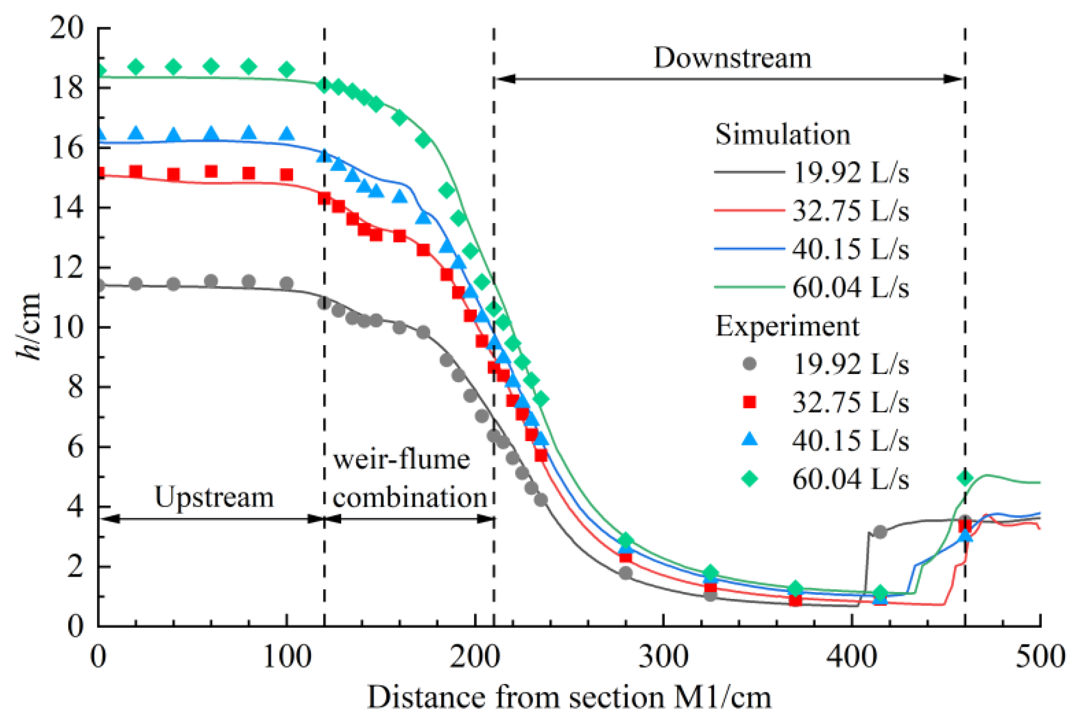
To evaluate the reliability of the numerical simulation, the simulated water-surface profiles were compared with the measured results obtained from the physical experiments. Four representative discharges, namely 19.92, 32.75, 40.15, and 60.04 L/s, were selected to cover both flume-flow and weir-flow regimes. Among them, 32.75 L/s corresponds to the experimentally identified flow threshold, while the other three cases represent low-flow, post-threshold, and high-flow conditions, respectively. As shown in Figure 8, the simulated water-surface profiles agree well with the experimental measurements under all selected discharges. In the upstream region, both the experimental and numerical results show a relatively stable water surface, indicating that the model successfully reproduces the backwater effect induced by the weir–flume combination facility. Within the contraction and trapezoidal sections, the numerical model captures the rapid decrease in water depth caused by flow acceleration. Downstream of the structure, both results show the formation of a thin water layer and local water-surface fluctuations, which are associated with flow separation, recirculation, and hydraulic-jump-like disturbances. Quantitatively, the relative errors between simulated and measured water depths were generally within 5% for all selected cases. The relatively larger deviations occurred mainly in the downstream thin-water-layer region, where the flow was highly turbulent and accompanied by strong free-surface fluctuations. Nevertheless, the numerical model accurately reproduced the overall trend of water-surface variation and the main hydraulic features observed in the laboratory tests. Therefore, the adopted Flow-3D model with the RNG k-ε turbulence closure was considered reliable for further analysis of the Froude number distribution, velocity field, and three-dimensional flow characteristics of the weir–flume combination facility.

Figure 8. Variation of water-surface line in the longitudinal profile of the channel centre under different flow rates.

3.2.2. Reliability Verification of Simulation

To verify the accuracy of the simulation results, the test and numerical simulation results along the water-surface line of the longitudinal profile of the facility under four flows (19.92 L/s, 32.75 L/s, 40.15 L/s and 60.04 L/s) inside and outside the flow threshold range were selected for comparison (Figure 8). It can be seen from Figure 8 that the simulation results of water-surface line changes along the four flow rates are consistent with the experiment. The maximum relative error of all conditions is less than 5%, indicating that the numerical simulation method used in this study is reasonable and reliable. The experimental Reynolds numbers were sufficiently large to ensure fully turbulent flow conditions, thereby minimizing potential scale effects associated with viscous forces. Considering the measurement uncertainties associated with water depth, discharge, and flow velocity, the observed deviations between numerical simulations and experimental measurements remain within the expected experimental uncertainty range. Therefore, the identified hydraulic characteristics and the subsequent discharge equations are not significantly affected by measurement errors.

3.2.3. Froude Number Distribution

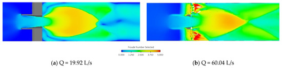
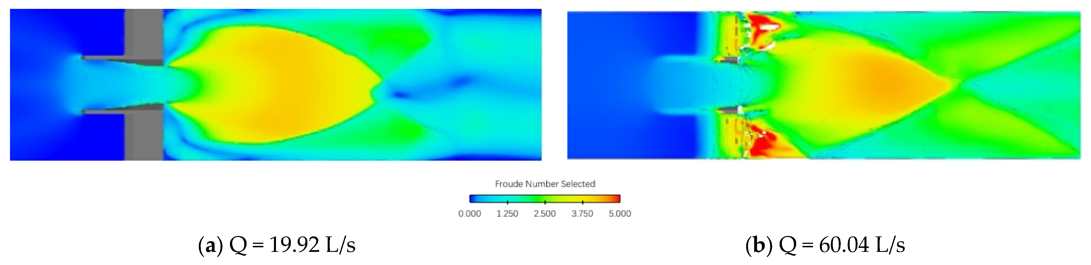
Froude number (Fr) is an important dimensionless number of open channel flow, which can be used as a criterion for judging the flow pattern. According to the simulation results, two typical cases (Q = 19.92 L/s and Q = 60.04 L/s, Figure 9) of the Fr distribution of the weir–flume combination facility are selected. The first case is that the flow only flows through the sluicing flume. As shown in Figure 9a, the Fr value increases first and then decreases along the way, reaching the maximum in the downstream thin-water layer area. In the upstream of the flume, the Froude number is less than 1, and the water flow is in a slow flow state. Fr gradually becomes larger after passing through the flume and is radially distributed in the thin-water layer area behind the flume, reaching a maximum of 4, and then gradually becomes smaller and develops downstream. In the second case, as shown in Figure 9b, the flow in the flume and the crest of the weir on both sides overflow simultaneously. Different from the first case, Fr has a maximum value of 5 in the scour area behind the weir on both sides. The radial distribution behind the flume is more concentrated by the constraints of the channels on both sides, showing a triangular distribution, and the Fr value is larger at the sharp corners. In the downstream of the weir–flume combination facility, the distribution is consistent with the flow pattern, showing the shape of the diamond wave.

Figure 9. Distribution of Fr under different flow rates.

3.2.4. Velocity Distribution

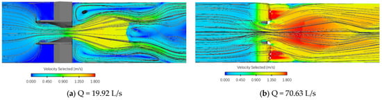
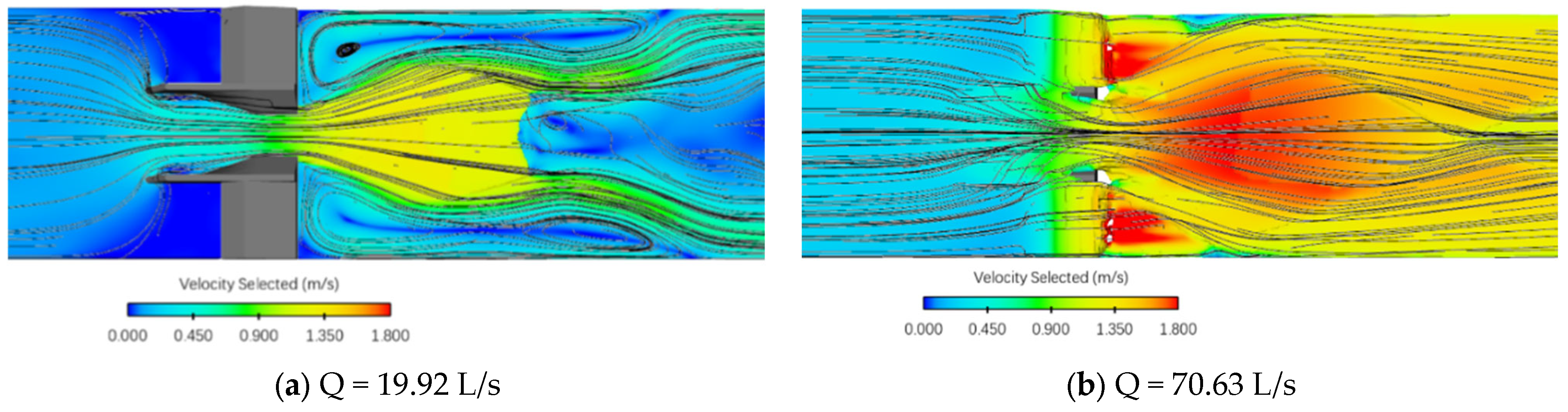
The velocity distribution reflects the hydrodynamic conditions related to flow acceleration, low-velocity recirculation and potential downstream scouring. As shown in Figure 10a, when the discharge is below the threshold, the flow velocity gradually increases from the upstream approach section to the weir–flume combination. This acceleration is mainly caused by the lateral contraction of the facility. As the effective flow width decreases in the torsional and trapezoidal sections, the same discharge must pass through a smaller cross-sectional area. According to the continuity equation, the mean velocity therefore increases, and the streamlines become progressively denser near the contracted section. This indicates that the weir–flume combination acts as a hydraulic control section, converting part of the pressure head into velocity head. After the flow leaves the flume outlet, the high-velocity jet enters the wider downstream channel. Due to the sudden lateral expansion, the streamlines spread radially outward. However, this expansion is restricted by the side walls of the channel, causing part of the flow to turn back toward the channel centerline. As shown in Figure 10b, when the discharge is above the threshold, the velocity field in the upstream section and inside the measuring flume still shows a similar acceleration and streamline-concentration process. However, the downstream flow pattern changes significantly after the flow passes through the facility. At this higher discharge, water overtops both sides of the weir crest. Part of the flow crosses the side wall of the excess-flow flume before entering the downstream region. Therefore, the downstream flow is no longer controlled only by the central flume jet, but also by the overflow from both sides of the weir. The interaction between the central high-velocity jet and the lateral overflow produces a stronger impact region downstream of the weir.

Figure 10. Distribution of flow velocity and streamlines.

3.3. Development of Discharge Formulas and Hydraulic Analysis

3.3.1. Development of the Discharge Equation for Flume Flow

Based on the principle of critical flow, this section derives the specific theoretical formula adapted to the geometry of the weir–flume combination. Unlike standard rectangular weirs, the critical flow condition in our structure occurs within a trapezoidal section. The following derivation establishes the basis for introducing the empirical discharge coefficient. From Fr = 1 of the critical flow section, the relationship between the average velocity of the critical section and the critical water depth is obtained (Equation (13)). Thus, the preliminary expression of the flow rate can be obtained as shown in Equation (14).

$${\mathrm{v}}_{\mathrm{cr}}=\sqrt{\mathrm{g}{\mathrm{h}}_{\mathrm{cr}}}$$

(13)

$$\mathrm{Q}={\mathrm{v}}_{\mathrm{cr}}·{\mathrm{A}}_{\mathrm{cr}}=\sqrt{\mathrm{g}{\mathrm{h}}_{\mathrm{cr}}}·{\mathrm{A}}_{\mathrm{cr}}={ \mathrm{b}}_{\mathrm{cr}}·\sqrt{\mathrm{g}}·{\mathrm{h}}_{\mathrm{cr}}^{1.5}$$

(14)

where v_cr is the critical flow velocity (m/s); hcr is the critical section depth (m); Q is the overcurrent flow (m³/s); A_cr is the critical section area (m²); and b_cr is the critical depth section width (m).

As can be seen from Figure 6, the position of the critical section water depth changes with flow rate, so it is difficult to determine its exact position. Therefore, a stable section is found in the upstream section of the measurement flume, and a stable relationship between flow rate and water depth is established through the energy equation and critical section water depth. Assuming that the energy loss of water depth of the upstream measurement point section and critical section is ignored, Equation (15) can be obtained according to the Bernoulli equation. Since the bottom elevation is the same, Equation (15) can be substituted into Equation (14) to obtain Equation (16).

$$\mathrm{E}={\mathrm{z}}_{\mathrm{i}}+{\displaystyle \frac{{\mathrm{v}}_{\mathrm{i}}^2}{2\mathrm{g}}}+{\mathrm{h}}_{\mathrm{i}}={\mathrm{z}}_{\mathrm{cr}}+{\displaystyle \frac{{\mathrm{v}}_{\mathrm{cr}}^2}{2\mathrm{g}}}+{\mathrm{h}}_{\mathrm{cr}}$$

(15)

$$\mathrm{Q}={\displaystyle \frac{2}{3}}\sqrt{{\displaystyle \frac{2}{3}}}{\mathrm{b}}_{\mathrm{cr}}\sqrt{\mathrm{g}}{\left({\mathrm{h}}_{\mathrm{i}}+{\displaystyle \frac{{\mathrm{v}}_{\mathrm{i}}^2}{2\mathrm{g}}}\right)}^{1.5}={\displaystyle \frac{2}{3}}\sqrt{{\displaystyle \frac{1}{3}}}{\mathrm{b}}_{\mathrm{cr}}\sqrt{2\mathrm{g}}{\mathrm{H}}_{\mathrm{i}}^{1.5}$$

(16)

where z_i is the bottom elevation of a section measurement point upstream (m); v_i is the average velocity of a measurement point in a section upstream (m/s); ${\mathrm{h}}_{\mathrm{i}}$ is the depth of a section measurement point upstream (m); z_cr is the critical depth section width (m); and ${\mathrm{H}}_{\mathrm{i}}$ is the total water head of a section measurement point upstream (m).

Since the derived equation (Equation (13)) is based on ideal energy conservation and neglects local energy losses, it must be calibrated with an empirical coefficient to reflect the actual hydraulic performance of the trapezoidal flume. The moving velocity coefficient is introduced to convert the full head ${\mathrm{H}}_{\mathrm{i}}$ into ${\mathrm{h}}_{\mathrm{i}}$. It can be seen from Figure 6 that the critical water depth section appears in the trapezoidal section of the sluicing flume, so b_cr = b. Simplify ${\displaystyle \frac{2}{3}}\sqrt{{\displaystyle \frac{1}{3}}}$ to 0.385. The final flow measurement formula is shown in Equation (17).

$$\mathrm{Q}=0.385·{\mathrm{C}}_{\mathrm{dv}}·\mathrm{b}·\sqrt{2\mathrm{g}}{·\mathrm{h}}_{\mathrm{i}}^{1.5}$$

(17)

where C_dv is a comprehensive flow coefficient considering the flow coefficient and velocity coefficient. Therefore, the identification of the trapezoidal section as the hydraulic control section is considered robust, whereas the precise location of the critical depth section under weir-flow conditions should be interpreted qualitatively because of the different Froude-number calculation approaches adopted in the present study.

3.3.2. Development of the Discharge Equation for Combined Weir–Flume Flow

When the flow rate is greater than the flow threshold, both sides of the Crump weir began to flow, so that we cannot continue to use the original flow formula. Some scholars have pointed out that the existing flow coefficient formula of the Crump weir is only suitable for the two-dimensional flow state of the streamline perpendicular to the weir top, and it is no longer applicable to the Crump weir with lateral flow [12]. In the experiment, it was found that when the flow rate was greater than the threshold, the side wall of the measurement flume began to flow, and there was obvious cross-flow at the top of the Crump weir. Therefore, the flow formula algorithm proposed by Wessels [19] has some errors. In the experiment, it is found that the flow mode of the weir–flume combination facility is similar to that of the labyrinth weir under the condition of side weir flow. Therefore, this paper regards the weir–groove combination as the combination of two L-shaped labyrinth weirs and combines the flow formula of the labyrinth weir and the Crump weir to obtain Equation (18).

$$\mathrm{Q}=0.385·{\mathrm{m}}_0·{\mathrm{L}}_{\mathrm{w}}·\sqrt{2\mathrm{g}}·{\mathrm{h}}_{\mathrm{w}}^{1.5}$$

(18)

where m₀ is the comprehensive flow coefficient when the flow is greater than the threshold flow; L_w is the effective water length of the weir–flume combination, which is the sum of the width of the Crump weir and the length of the side wall of the measurement flume (m); and h_w is the water depth above the crest elevation in the upstream of the weir–flume combination (m).

3.3.3. Calibration of Empirical Discharge Coefficients

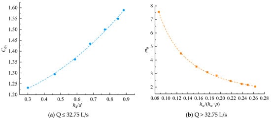
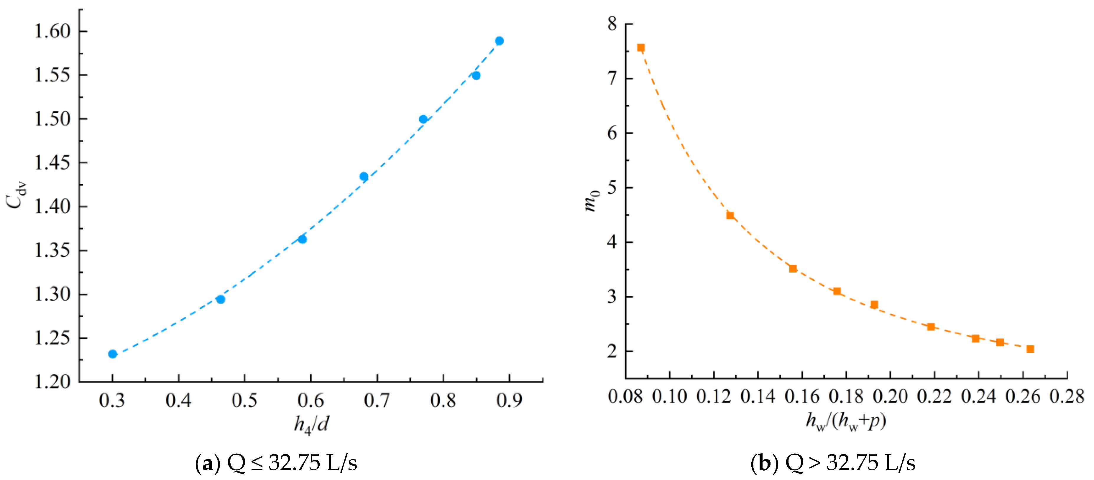
According to the experimental data, the water depth of five measurement points (measurement points 1–5) in the inlet section of the sluicing flume is fitted with the calculated comprehensive flow coefficient. It is found that the correlation between measurement point 4 and the comprehensive flow coefficient is the strongest, and the multiple correlation coefficient is 0.998, so measurement point 4 is used as the water level measurement point within the flow threshold range. Figure 11a shows that the comprehensive flow coefficient C_dv changes with the relative water depth of measurement point 4 when the flow is less than the threshold flow. It can be seen from Figure 11a that the comprehensive flow coefficient C_dv increases with the increase of the relative water depth h₄/d. The empirical formula expression of the comprehensive flow coefficient of the flume with discharge capacity was obtained by fitting (Equation (19)).

Figure 11. Variation of comprehensive flow coefficient with relative acting head.

Figure 11b shows the change of the comprehensive flow coefficient m₀ with the relative action of water head h_w/(h_w + p) at measurement point M1 when the flow rate is greater than the flow threshold. As can be seen from Figure 11b, the flow coefficient decreases with the increase of h_w/(h_w + p). Equation (20) was obtained by formula fitting for m₀ according to the test data, and the correlation of its complex correlation coefficient reached 0.999.

$${\mathrm{C}}_{\mathrm{dv}}=0.4447{\left({\mathrm{h}}_4/\mathrm{d}\right)}^2+0.0866\left({\mathrm{h}}_4/\mathrm{d}\right)+1.162\hspace{1em}{\mathrm{h}}_4/\mathrm{d}\le 0.885$$

(19)

$${\mathrm{m}}_0=0.9658+0.1269{\left({\displaystyle \frac{{\mathrm{h}}_{\mathrm{w}}}{{\mathrm{h}}_{\mathrm{w}}+\mathrm{p}}}\right)}^{-1.6180}\hspace{1em}{\mathrm{h}}_4/\mathrm{d}>0.885$$

(20)

where h₄ is the water depth of measurement point 4 (m); d is the wall height of the sluicing flume (m); and h_w is the water depth above the weir crest elevation upstream of the weir–flume combination (m). In this study, h_w = h_M1-p, h_M1 is the water depth of the upstream measurement point M1 (m); p is the weir height of Crump weirs on both sides. The comparison among Measurement Points 1–5 indicates that Point 4 provides the highest correlation with the discharge coefficient and exhibits the most stable hydraulic response. Therefore, it was selected not only for the discharge equations but also as the reference point for defining the flow-regime transition criterion.

3.3.4. Hydraulic Relationship Between Measurement Points 4 and M1

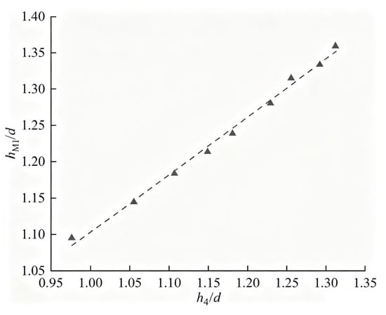
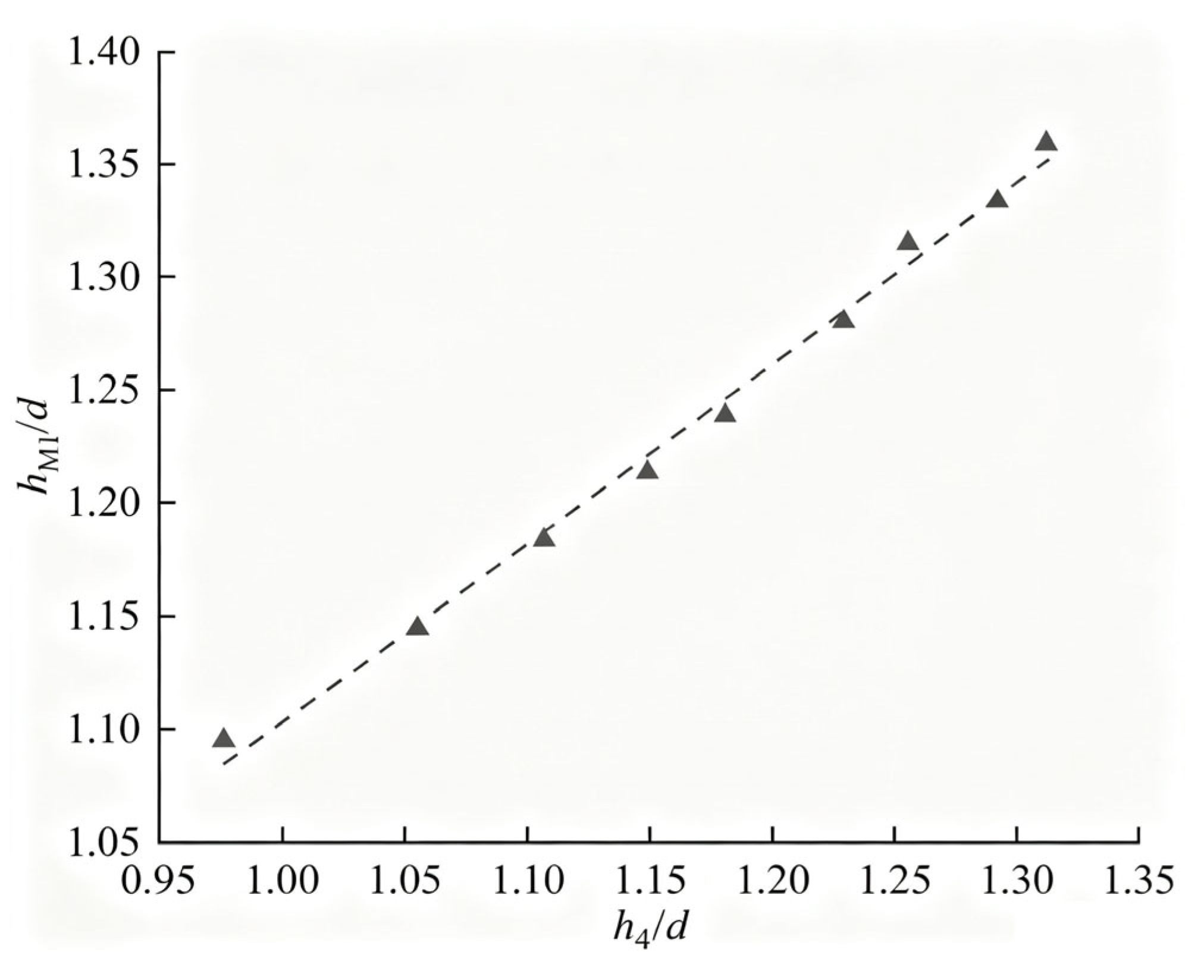
When the flow is greater than the flow threshold, based on the water depth hM1 of the upstream measurement point M1, the flow coefficient m₀ under the condition of different outlet widths of the flume can be obtained by substituting it into the previous formula (17). Then, the flow rate can be calculated according to formula (4). However, in the model test, it is found that the upstream section before the inlet of the weir trough combination water measurement facility has a low flow velocity, so a certain degree of sediment deposition will be generated in this section, which will affect the measurement accuracy of the depth measurement point M1. However, the flow velocity in the measurement trough is larger and it is not prone to siltation, so it is necessary to find a depth of water depth of the measurement point M1 in the trough instead of the water depth of the upstream measurement point M1. This interpretation is consistent with the experimental observation that the measuring flume maintains relatively high flow velocities, making sediment deposition less likely within the measurement section compared with the upstream approach channel. Figure 12 shows the relationship between the water depth of measurement points 4 and M1. It can be seen from the figure that the water depth of measurement point M1 increases with the increase of the water depth of measurement point 4, and the water depth of the two has a significant linear relationship. At the same time, since the flow coefficient fitting formula and flow formula of the flow in the trough are based on measurement point 4, replacing the water depth of measurement point M1 with the water depth of measurement point 4 can not only ensure the accuracy requirements of the flow formula but also simplify the measurement steps. The empirical formula for the relative action of the water head between measurement point M1 and measurement point 4 is shown in Equation (21). The correlation coefficient between them is 0.994.

(h_M1/d) = 0.7964(h₄/d) + 0.3067

(21)

Figure 12. Relative water depth relationship between measurement point 4 and measurement point M1.

4. Discussion

4.1. Flow Formula and Measurement Accuracy Verification

By substituting Equation (21) into Equations (20) and (18), the flow formula of weir flow can be obtained. At the same time, the flow formula (17) of the flow in the flume and the empirical formula (16) of the flow coefficient can be summarized. After sorting out, the flow calculation formulas within and outside the flow threshold range can be obtained, as shown in Equations (22) and (23).

$$\mathrm{Q}=0.385·{\mathrm{C}}_{\mathrm{dv}}·\mathrm{b}·\sqrt{2\mathrm{g}}{·\mathrm{h}}_4^{1.5}\hspace{1em}{\mathrm{C}}_{\mathrm{dv}}=0.4447{\left({\mathrm{h}}_4/\mathrm{d}\right)}^2+0.0866\left({\mathrm{h}}_4/\mathrm{d}\right)+1.1629\hspace{1em}{\mathrm{h}}_4/\mathrm{d}\le 0.885$$

(22)

$$\mathrm{Q}={\mathrm{m}}_0·{\mathrm{L}}_{\mathrm{w}}·0.385·\sqrt{2\mathrm{g}}·{\left(0.7964{\mathrm{h}}_4+0.3067\mathrm{d} - \mathrm{p}\right)}^{1.5}\hspace{1em}{\mathrm{m}}_0=0.9658+0.1269{\left(1 -{\displaystyle \frac{\mathrm{p}}{{0.7964\mathrm{h}}_{4 }+0.3067\mathrm{d}}}\right)}^{-1.6180}\hspace{1em}{\mathrm{h}}_4/\mathrm{d}>0.885$$

(23)

The water depth of measuring point 4 under 14 working conditions in the model test was substituted into the above flow calculation formula to obtain the calculated flow value, and the calculated flow value was compared with the measured value. The results are shown in Table 2. As can be seen from Table 2, the maximum relative errors of traffic calculated within and outside the traffic threshold range are 0.52% and −2.15%, respectively. On the whole, all the relative errors are less than 3%, which meets the measurement requirements. However, mountainous rivers typically involve higher Reynolds numbers, stronger bed-roughness effects, air entrainment, non-uniform hydraulic response, and highly three-dimensional turbulence. Therefore, the experimental results are intended to reveal qualitative trends and comparative hydraulic behavior under controlled conditions. Before the results can be quantitatively applied to prototype mountainous rivers, further validation using higher discharges, a wider range of hydraulic conditions, field measurements, or numerical simulations is required. Although measurement uncertainties are inevitable in hydraulic experiments, their magnitudes are substantially smaller than the hydraulic differences observed among the tested discharge conditions. Water depth, discharge, and flow velocity were measured using calibrated instruments, and repeated measurements were performed after the flow reached steady conditions to reduce random errors. Consequently, these uncertainties do not affect the identification of the flow transition threshold, the observed hydraulic characteristics, or the fitting accuracy of the proposed discharge equations.

Table 2. Comparison results of measured discharge value and calculated discharge value under different water.

(h4) cm	Measured Discharge/(L∙s−1)	Calculated Discharge/(L∙s−1)	Relative Error/%
4.51	5.03	5.02	−0.22
6.96	10.13	10.17	0.37
8.81	15.19	15.24	0.34
10.20	19.92	19.82	−0.48
11.55	25.10	24.99	−0.44
12.75	30.08	30.24	0.52
13.27	32.75	32.72	−0.10
14.67	40.15	39.29	−2.15
15.84	45.15	45.72	1.26
16.60	50.30	51.03	1.45
17.22	55.12	55.86	1.34
17.69	60.04	59.77	−0.44
18.42	65.20	66.25	1.61
18.79	70.63	69.71	−1.31
19.35	74.90	75.14	0.32
19.64	78.70	78.04	−0.84

In natural mountain rivers, coarse sediment, gravel, and bed roughness are expected to modify the local hydraulic characteristics of the weir–flume combination facility. Increased bed roughness generally leads to greater energy dissipation and lower flow velocities upstream of the structure, while sediment deposition may alter the effective cross-sectional geometry and consequently influence the stage–discharge relationship. In addition, gravel transport during high-flow events may locally modify the hydraulic control conditions near the flume entrance or downstream thin-water-layer region. Nevertheless, the proposed structure possesses several features that may reduce these influences. The central flume maintains relatively high flow velocities, which are beneficial for limiting sediment deposition within the measuring section, while the Crump weir promotes stable hydraulic control over a wide range of discharges. Therefore, although the quantitative discharge equations should be further calibrated for prototype rivers with different roughness and sediment conditions, the hydraulic mechanisms identified in this study are expected to remain applicable. Future work will incorporate movable-bed experiments and field-scale verification under different hydraulic response conditions to further evaluate the hydraulic and operational performance of the proposed facility.

4.2. Limitations and Future Work

The present study was conducted under laboratory-scale conditions; thus, scale effects should be considered when interpreting the results. In open-channel flows dominated by gravity, the Froude number is the primary similarity criterion governing dynamic similarity between laboratory and prototype systems. In this study, the experimental conditions were designed to maintain consistent Froude-controlled flow behavior across different discharge cases. Meanwhile, the Reynolds numbers in all tests were sufficiently high to ensure fully developed turbulent flow, reducing the influence of viscous effects on the hydraulic behavior of the weir–flume system. Although minor discrepancies due to geometric scaling and wall effects may still exist, their impact on the key hydraulic parameters, including the relative water depth threshold (0.885) and the derived discharge equations, is considered limited. It should be noted that the present study does not aim to identify or analyze a fully developed hydraulic jump. Therefore, no specific energy-loss analysis or conjugate-depth calculation was performed. Some terms are used only to qualitatively describe the observed free-surface fluctuations and turbulent flow structures.

Compared with conventional Crump weirs or existing flume structures, the proposed facility is characterized not merely by combining two existing hydraulic structures, but by establishing a hydraulically integrated configuration in which the central measuring flume and the side weirs perform complementary hydraulic functions under different discharge conditions. The flume dominates discharge measurement under low-flow conditions, whereas the side Crump weirs gradually participate in flow conveyance after the threshold discharge is exceeded. This transition mechanism distinguishes the proposed facility from conventional flow-measurement structures and forms the basis for the segmented discharge equations established in this study. Therefore, while direct quantitative extrapolation to natural mountain rivers requires caution, the identified hydraulic mechanisms and dimensionless relationships are expected to remain valid at prototype scale after appropriate field calibration. Future work should further validate these findings through prototype measurements and large-scale experimental studies.

It should be noted that the proposed discharge equations are applicable to hydraulic conditions similar to those investigated in the present study. Specifically, the equations are valid for free outflow conditions and the tested discharge range (5–79 L/s). The flow regime is distinguished using the relative water-depth criterion (h₄/d = 0.885), corresponding to flume flow and combined weir–flume overflow, respectively. The equations were established based on the geometric configuration of the proposed facility and should therefore be applied to structures with similar geometric proportions. In addition, the equations are intended for gravity-dominated open-channel flows in which the Froude number distributions are consistent with those observed in the present experiments. Application outside these hydraulic or geometric conditions should be accompanied by additional calibration or verification. And the threshold value h₄/d = 0.885 was derived for the specific geometric configuration investigated in this study. Although the dimensionless form improves its applicability, the threshold should be regarded as geometry-dependent and requires recalibration for substantially different weir heights, flume widths, or geometric proportions.

5. Conclusions

This study investigated the hydraulic characteristics and flow-measurement performance of a weir–flume combination facility through laboratory experiments and Flow-3D numerical simulations under free outflow conditions over a discharge range of 5–79 L/s. The results demonstrated that the facility exhibits two distinct hydraulic regimes, namely flume flow and combined weir–flume overflow, with a transition occurring at a discharge of 32.75 L/s, corresponding to a relative water depth of h₄/d = 0.885. This dimensionless threshold provides a practical criterion for identifying the flow-regime transition and forms the basis for establishing segmented discharge equations. The numerical simulations reproduced the measured water-surface profiles with relative errors generally below 5%, confirming that the adopted Flow-3D model coupled with the RNG k–ε turbulence model can reliably capture the hydraulic behavior of the proposed facility within the investigated hydraulic conditions.

The combined experimental and numerical analyses further revealed that the flow field is characterized by strong three-dimensional hydraulic features downstream of the structure, including rapid flow acceleration, thin-water-layer development, and localized free-surface disturbances associated with hydraulic-jump-like flow behavior. Based on these hydraulic characteristics, separate discharge equations were established for the flume-flow and weir-flow regimes. The empirical discharge coefficients exhibited clear relationships with the relative water depth and relative upstream head, enabling accurate calibration of the proposed equations. Validation against the experimental measurements showed that the calculated discharges agreed well with the measured values, with relative errors generally below 3%, indicating that the proposed equations satisfy the accuracy requirements for flow measurement under the tested conditions.

The proposed weir–flume combination facility provides a practical approach for extending the measurable discharge range while maintaining stable hydraulic control. Nevertheless, the present study was conducted under laboratory-scale conditions and for a specific geometric configuration. Therefore, the proposed threshold criterion and discharge equations should be regarded as geometry-dependent and require recalibration before application to substantially different structural configurations or natural mountain rivers with different sediment conditions, channel roughness, and hydraulic environments. Future studies should focus on prototype-scale verification, movable-bed experiments, and field applications to further evaluate the hydraulic performance and long-term applicability of the proposed facility.

References

- Tao, F.; Xiao, B.; Qi, Q.; Cheng, J.; Ji, P. Digital twin modeling. J. Manuf. Syst. 2022, 64, 372–389. [Google Scholar] [CrossRef] [Scilit]
- Tao, F.; Qi, Q. Make more digital twins. Nature 2019, 573, 490–491. [Google Scholar] [CrossRef] [Scilit] [PubMed]
- Tao, F.; Zhang, H.; Liu, A.; Nee, A.Y.C. Digital twin in industry: State-of-the-art. IEEE Trans. Ind. Inform. 2019, 15, 2405–2415. [Google Scholar] [CrossRef] [Scilit]
- Grieves, M.; Vickers, J. Digital Twin: Mitigating Unpredictable, Undesirable Emergent Behavior in Complex System; Springer: Berlin/Heidelberg, Germany, 2017. [Google Scholar]
- Ye, Y.; Jiang, Y.; Liang, L.; Zhao, H.; Gu, J.; Dong, J.; Cao, Y.; Duan, H. Digital twin watershed: New infrastructure and new paradigm of future watershed governance and management. Adv. Water Sci. 2022, 33, 683–704. (In Chinese) [Google Scholar]
- Azimi, A.H.; Hakim, S.S. Hydraulics of flow over rectangular labyrinth weirs. Irrig. Sci. 2019, 37, 183–193. [Google Scholar]
- Erick, M.; Jorge, F.; Waldo, O.; Carlos, D.; Humberto, S. Influence of crest geometric on discharge coefficient efficiency of labyrinth weirs. Flow Meas. Instrum. 2021, 81, 101955. [Google Scholar] [CrossRef] [Scilit]
- Aylar, S.; Farzin, S.; Hadi, A.; Maysam, M. Effects of geometrical parameters on labyrinth weir hydraulics. J. Irrig. Drain. Eng. 2022, 148, 04022032. [Google Scholar] [CrossRef] [Scilit]
- Yousef, S.; Hassan, T.; Masoud, G.; Mojtaba, M.; Reza, Z. Hydrodynamics and free-flow characteristics of piano key weirs with different plan shapes. Water 2021, 13, 2076. [Google Scholar] [CrossRef] [Scilit]
- Shen, X.; Oertel, M. Comparative study of nonsymmetrical trapezoidal and rectangular piano key weirs with varying key width ratios. J. Hydraul. Eng. 2021, 147, 04021046. [Google Scholar] [CrossRef] [Scilit]
- Longo, S. Experiments on turbulence beneath a free surface in a stationary field generated by a Crump weir: Free-surface characteristics and the relevant scales. Exp. Fluids 2010, 49, 1325–1338. [Google Scholar] [CrossRef] [Scilit]
- Zuikov, A.L. Hydraulics of the classical Crump weir water gauge. Power Technol. Eng. 2017, 50, 611–619. [Google Scholar] [CrossRef] [Scilit]
- AL-Naely, H.; Al-Khafaji, Z.; Khassaf, S. Effect of opening holes on the hydraulic performance for Crump weir. Int. J. Eng. 2018, 31, 2022–2027. [Google Scholar] [CrossRef] [Scilit]
- Russon, I.J.; Kemp, P.S.; Lucas, M.C. Gauging weirs impede the upstream migration of adult river lamprey Lampetra fluviatilis. Fish. Manag. Ecol. 2011, 18, 201–210. [Google Scholar]
- Ghimire, S.; Jones, G. Restoration of a gauging weir to aid fish passage. J. Hydro-Environ. Res. 2014, 8, 43–49. [Google Scholar] [CrossRef] [Scilit]
- Montali-Ashworth, D.; Vowles, A.S.; De Almeida, G.; Kemp, P.S. Use of cylindrical bristle clusters as a novel multispecies fish pass to facilitate upstream movement at gauging weirs. Ecol. Eng. 2020, 143, 105670. [Google Scholar] [CrossRef] [Scilit]
- Javier, S.F.; Javier, B.F.; Ana, G.; Jorge, V.; Andrés, M.; Francisco, F.J. Fish upstream passage through gauging stations: Experiences with Iberian barbel in flat-V weirs. Fishes 2021, 6, 55. [Google Scholar] [CrossRef] [Scilit]
- Wessels, P.; Rooseboom, A. Flow-gauging structures in South African rivers Part 1: An overview. Water SA 2012, 35, 1–9. [Google Scholar] [CrossRef] [Scilit]
- Wessels, P.; Rooseboom, A. Flow-gauging structures in South African rivers Part 2: Calibration. Water SA 2012, 35, 11–19. [Google Scholar] [CrossRef] [Scilit]
- Sun, B.; Yang, L.; Zhu, S.; Liu, Q.; Wang, C.; Zhang, C. Study on the applicability of four flumes in small rectangular channels. Flow Meas. Instrum. 2021, 80, 101944. [Google Scholar] [CrossRef] [Scilit]
- Li, X.; Jin, L.; Engel, B.A.; Yang, Z.; Wang, W.; He, W.; Wang, Y. Influence of the structure of cylindrical mobile flumes on hydraulic performance characteristics in U-shaped channels. Flow Meas. Instrum. 2020, 72, 101711. [Google Scholar] [CrossRef] [Scilit]
- Said, M.B.; Ouamane, A. Performance of rectangular labyrinth weir—An experimental and numerical study. Water Supply 2022, 22, 3628–3644. [Google Scholar] [CrossRef] [Scilit]
- Ali, Y.; İhsan, M.A.; Mustafa, G. Numerical and experimental modelling of flow at Tyrolean weirs. Flow Meas. Instrum. 2021, 81, 101954. [Google Scholar] [CrossRef] [Scilit]
- Hanifeh, I.; Abdolmajid, M.; Pouneh, H. Experimental and numerical study of flow over a broad-crested weir under different hydraulic head ratios. Flow Meas. Instrum. 2021, 80, 101945. [Google Scholar] [CrossRef] [Scilit]
- Mason, G.; Robert, E. Effect of clearwater scour on the flow field at a single bendway weir: Two-dimensional numerical modeling supported by flume data. J. Irrig. Drain. Eng. 2021, 147, 04021001. [Google Scholar] [CrossRef] [Scilit]
- Fuentes-Pérez, J.F.; Quaresma, A.L.; Pinheiro, A.; Sanz-Ronda, F.J. OpenFOAM vs FLOW-3D: A comparative study of vertical slot fishway modelling. Ecol. Eng. 2022, 174, 106439. [Google Scholar] [CrossRef] [Scilit]
- Aghaei, Y.; Kilanehei, F.; Faghihrad, S.; Nazari-Sharabian, M. Dynamic pressure at flip buckets of chute spillways: A numerical study. Int. J. Civ. Eng. 2022, 20, 421–432. [Google Scholar]
- Versteeg, H.K.; Malalasekera, W. An Introduction to Computational Fluid Dynamics: The Finite Volume Method; Pearson Education: London, UK, 2007. [Google Scholar]
- Ran, D.; Wang, W.; Hu, X. Three-dimensional numerical simulation of flow in trapezoidal cutthroat flumes based on FLOW-3D. Front. Agric. Sci. Eng. 2018, 5, 168–176. [Google Scholar] [CrossRef] [Scilit]
- Wang, Y.; Wang, W.; Hu, X.; Liu, F. Experimental and numerical research on trapezoidal sharp-crested side weirs. Flow Meas. Instrum. 2018, 64, 83–89. [Google Scholar] [CrossRef] [Scilit]
- Chiu, C.L.; Fan, C.M.; Tsung, S.C. Numerical modeling for periodic oscillation of free overfall in a vertical drop pool. J. Hydraul. Eng. 2017, 143, 04016077. [Google Scholar] [CrossRef] [Scilit]
- Shen, X.; Li, R.; Cai, H.; Feng, J.; Wan, H. Characteristics of secondary flow and separation zone with different junction angle and flow ratio at river confluences. J. Hydrol. 2022, 614, 128537. [Google Scholar] [CrossRef] [Scilit]
Disclaimer/Publisher’s Note: The statements, opinions and data contained in all publications are solely those of the individual author(s) and contributor(s) and not of MDPI and/or the editor(s). MDPI and/or the editor(s) disclaim responsibility for any injury to people or property resulting from any ideas, methods, instructions or products referred to in the content. |
© 2026 by the authors. Licensee MDPI, Basel, Switzerland. This article is an open access article distributed under the terms and conditions of the Creative Commons Attribution (CC BY) license.