


Abstract
Slope stability has consistently been a critical concern in mountainous road sections, with precipitation being the most significant factor precipitating slope instability. This study aims to elucidate the mechanism of slope instability under precipitation conditions and the extent of the impact of internal disaster-causing factors. To achieve this objective, a numerical simulation analysis method combining GeoStudio2018R2 and FLAC3D7.0 software was employed to conduct a comprehensive analysis of an unstable slope in Xinjiang. Regarding research methodology, cyclic precipitation and seasonal snowmelt were considered as external influencing factors. Initially, a two-dimensional model was constructed using GeoStudio software to analyze the spatial and temporal variations in pore water pressure and moisture content within the slope, elucidating their dynamic characteristics at different temporal and spatial scales. Subsequently, a three-dimensional numerical model was established using FLAC3D software to conduct a detailed analysis of the stress–strain state of the slope under various conditions, thereby obtaining disaster parameters such as displacement and sliding velocity in different directions. Through further comparison and verification of the overall stability analysis results of the slope obtained from both software packages, it was observed that they exhibited a consistent trend. The research findings indicate that under conditions of high-intensity short-term precipitation, the safety factor of the slope decreases to the lowest level, potentially leading to shallow landslides with smaller displacement but faster sliding velocity. Conversely, seasonal snowmelt and long-term localized precipitation have a more profound impact on the internal structure of the slope, with the sliding zone potentially penetrating into the deep bedrock. Although the occurrence frequency is low, the impact range is extensive. By combining two-dimensional and three-dimensional analyses, a comprehensive assessment of the different disaster-causing factors of the slope was conducted, enhancing the accuracy of the analysis results. The research findings provide a scientific basis and reference value for the formulation of subsequent slope protection and monitoring plans.
1. Introduction
Landslides are significant hazards in the western regions of China, with a wide range of triggering factors. Data from 2010 to 2018 indicate that Xinjiang experienced 302 geological disasters, including 136 landslides. Recent reports have highlighted the severe impact of landslides in China, such as an incident in Yunnan Province where dozens of people were buried, resulting in a high death toll [1]. According to incomplete statistics, in 2023, there were 36 significant landslides in Xinjiang, resulting in the destruction of dozens of roads and the demolition of multiple infrastructure facilities. These events underscored the urgent need for research into mechanisms of landslide formation and preventive measures. However, varied geological conditions lead to differences in the mechanisms of landslide formation. For example, rock landslides are typically caused by sliding along rock layers [2], characterized by distinct slip surfaces and rapid movement, whereas soil landslides often occur due to reduced soil shear strength, featuring less distinct slip surfaces and slower movement [3,4]. From debris landslides to loess and permafrost landslides, each type of geological condition gives rise to unique mechanical properties and structural characteristics that determine the diversity and specificity of landslide mechanisms [5,6]. Therefore, analyzing the mechanisms of landslides under specific geological conditions is crucial for regional prevention and management.
The main external factors contributing to landslide occurrence include rainfall, earthquakes, surface fissures, and mining, with rainfall being the most influential factor [7,8]. Internal factors primarily involve the lithological characteristics, strength, and permeability of different stratigraphic layers within geological regions, as well as the distribution, orientation, and nature of structural features, such as fissures, joints, and faults in rock bodies, which play a decisive role in landslide initiation [9,10]. Regarding the factors influencing landslides, Crosta et al. investigated a landslide in northern Italy by studying the meteorological events triggering soil slippage based on lithology to determine rainfall thresholds and assess regional conditions using soil properties, triggering rainfall, and the local lithological environment [11]. Ozdemir et al. constructed a sensitivity map near the Yaka landslide in Turkey by analyzing factors such as lithology, gradient, slope aspect, elevation, topographic wetness index, and stream power index [12]. Berhane et al. aimed to generate a landslide sensitivity map for the Mgulat mountainous area in Ethiopia by considering factors such as lithology, slope steepness, distance from drainage, land use, land cover, and slope aspect [13].
To date, scholars, both domestically and internationally, have achieved substantial research outcomes in the study of landslides. Common investigative methods include geological surveys, remote sensing imaging, borehole core analysis, lithological parameter analysis, rainfall data analysis, numerical simulations, and machine learning [14,15]. These methods aim to examine the geomorphological and stratigraphic characteristics of landslides, the causes of reactivation, and the dynamic mechanisms driving landslide occurrence [14]. Su et al. have utilized geophysical parameters such as shear wave velocity and resistivity to study the hydrogeological features of landslides, providing information on potential slip surfaces and groundwater seepage systems. They also conducted geological field surveys to study the deformation and failure modes of landslides and predict their stability [16]. Traditional investigation methods are accurate for landslide analysis, but can be complex and time-consuming, require significant human and equipment resources, and are not suitable for slopes in severe terrain conditions. At present, landslide numerical simulation is primarily used to investigate landslide mechanisms, predict occurrences, and assess stability and risk, serving as a crucial tool for understanding and mitigating landslide disasters. In particular, finite element modeling has been widely applied in landslide research to predict flow and related parameters [17].
Apart from finite element methods, the finite difference method (FDM) has also been extensively employed in landslide research due to its robustness in handling large deformation problems and complex boundary conditions. The commercial code FLAC3D (Fast Lagrangian Analysis of Continua in 3D), developed by Itasca Consulting Group, is a widely adopted tool that implements the explicit finite difference method for geotechnical analysis. Numerous studies have applied FLAC3D to investigate slope stability under various triggering conditions. For instance, Ma et al. employed the three-dimensional finite difference code FLAC3D to analyze the stability of a high loess slope, demonstrating that seepage flow significantly influences slope stability and can lead to abrupt failure when groundwater conditions change [18,19]. For rainfall-induced landslides, researchers have combined unsaturated–saturated seepage analysis with FLAC3D to evaluate slope response under heavy precipitation, taking into account the heterogeneity of weathered soil layers [20,21]. Chang et al. conducted stability analysis on a landslide group using both the limit equilibrium method and FLAC3D, concluding that FLAC3D offers a more straightforward approach to assess the dangerous slip surface and the corresponding safety factor [22]. The finite difference code has also been successfully applied to analyze the water-heat-mechanics coupling in slopes under extreme snow hazard conditions, providing insights into freezing depth and frost heaving deformation [23]. Furthermore, combined approaches integrating GeoStudio for seepage modeling and FLAC3D for stress–strain analysis have proven effective in evaluating landslide stability under complex hydrological conditions, as demonstrated by research on the Ganhaizi landslide in the Dadu River Basin, where the finite difference method successfully captured the stress–strain features of both shallow and deep sliding bodies [24].
With specific regard to the GeoStudio software package, which integrates the SEEP/W module for seepage analysis and the SLOPE/W module for limit equilibrium stability analysis, a substantial body of research has validated its applicability in landslide assessment. For example, Liu et al. employed the SLOPE/W and SEEP/W modules of GeoStudio to simulate slope stability under extreme rainstorm conditions at the Zhonggutai landslide site, revealing that water serves as the critical inducing factor and that the safety factor decreases significantly within the first four hours of continuous rainfall [25]. Wang et al. have demonstrated the utility of GeoStudio for landslide stability analysis, noting its convenience in calculating the stability coefficient and its capability to intuitively represent potential slip surfaces [26]. Most recently, a three-dimensional probabilistic framework for unsaturated slope stability assessment under rainfall infiltration has been developed using GeoStudio, with the SEEP3D module performing seepage analysis and the 3D simplified Bishop method coupled with Monte Carlo simulations to evaluate the factor of safety and the probability of failure [27].
The comparison between two-dimensional and three-dimensional numerical models has always been of interest in the field of geotechnical engineering. Domej et al. conducted a study on the numerical 2D and 3D models of the Diezma landslide in southern Spain [28]. This study applied seismic scenarios to simplified and smoothed 2D models to analyze the behavior of landslides under different conditions. He et al. focused on using 2D-RAPID and LS-RAPID 3D models to simulate rapid- and long-distance moving landslides [29]. The purpose of this study was to validate and compare these two models by applying them to actual landslide events in the Philippines. The results of this study provide insights into the effectiveness of 2D and 3D models in simulating landslide events. This comparison highlights the differences in the modeling methods and their implications for thermal control systems. Overall, the choice between two-dimensional and three-dimensional numerical models depends on the specific application and level of detail required for the analysis. While 2D models may be sufficient for some scenarios, 3D models offer a more comprehensive understanding of complex phenomena, such as landslides. For further research on landslides, 2D models provided clearer responses to the overall changes within the slope. For example, Shan et al. employed two-dimensional modeling to interpret geophysical and geotechnical engineering data for delineating the quick clay at a landslide site in Sweden [30]; Do et al. integrated a two-dimensional seepage model, a two-dimensional slope stability model, and a landslide dam geometry assessment model to analyze the formation of rainfall-induced landslide dams [31]. On the other hand, 3D approaches often involve finite element and discrete element analyses of large deformations and fracture behaviors, simulating the stress, strain, and displacement of slopes under loading. This includes analyzing the stress–strain state of the slope by dividing the continuous medium into a finite grid. Stead et al. used a three-dimensional finite element model to describe the stress and strain within a landslide more accurately, and some models incorporated constitutive relationships to describe the shear stress–strain behavior [32]. Additionally, such analytical models have been used to study the initiation of landslides, with Meijer focusing on the root tensile stress and strain relationship through a 3D model [33]. Although some studies have used 2D models to describe the stress field in natural landscapes, it has been noted that these models may not fully capture the complexity of the three-dimensional stress distribution. This study combined 2D and 3D models to develop and apply both models to analyze stress–strain behavior and internal hydraulics in landslides, aiming to improve the accuracy of exploring landslide behavior in complex terrains [34].
Previous studies have typically relied on either 2D limit equilibrium or 3D stress--strain analyses in isolation, with few integrating both to capture coupled hydrological-mechanical responses under mixed rainfall--snowmelt conditions. Moreover, investigations in the Ili region have largely treated rainfall and snowmelt-triggered landslides separately, ignoring their combined effects under cyclic precipitation. The present study overcomes these limitations as follows: (i) developing a coupled 2D-3D framework linking transient seepage (GeoStudio) with explicit stress--strain analysis (FLAC3D); (ii) incorporating three precipitation scenarios (prolonged snowmelt, high-intensity short-duration rainfall, and mixed rainfall); and (iii) quantitatively comparing safety factor evolution, displacement fields, and sliding mechanisms [35]. The combined approach offers three benefits: the 2D model provides rapid computation of pore water pressure and safety factor trends under wetting-drying cycles; the 3D model captures deformation extent, slip surface location, and displacement vectors unavailable in 2D; and cross-validation between the two software packages enhances result reliability. New insights include the following: (a) high-intensity short-duration rainfall triggers shallow, fast-moving landslides with the lowest safety factor; (b) seasonal snowmelt and long-duration low-intensity rainfall induce deeper slip surfaces with larger impact area; and (c) the safety factor decline exhibits a lag effect during rain-free periods. These findings provide a scientific basis for prioritizing protection measures according to regional precipitation types [36,37].
2. Overview of the Study Area
2.1. Geological Conditions
As shown in Figure 1, the study area is located on the right bank of Gongnaisi Gully along the G218 National Highway in Yili, Xinjiang (downstream direction). The landslide mass has a fan-shaped plane, resembling a banana leaf. The rear edge of the landslide exhibits a distinctive armchair-shaped topography, with a 30 m high backwall. The top of the landslide is the third-order terrace of the Gongnaisi River, and the toe of the landslide is a wide, gentle platform. The front edge of the landslide is tongue-shaped and approaches the G218 National Highway. The landslide has a transverse width of approximately 66 m and a longitudinal length of about 85 m, with a thickness of 8.1–14.9 m. The main sliding direction is 30°, and the landslide volume is approximately 4.9 × 10⁴ m3, classifying it as a translational mid-sized landslide.
Figure 1.
Overview of landslides.
Based on geological mapping, drilling, and trenching investigations, the stratigraphic lithology of the study area is primarily characterized by the following layers, as shown in Figure 2:
Figure 2.
Cross-sectional diagram of lithological stratigraphy.
- Gravel Layer: Multicolored, dense aggregate structure with moderate roundness. The general grain size ranges from 20 to 60 mm, with a maximum grain size of 110 mm, accounting for approximately 60% of the total volume. The parent rocks consist of limestone, andesitic porphyry, and sandstone, with fillers of rounded gravel and sandy soil. Drilling reveals a thickness of 5.00 to 10.00 m.
- Fully Weathered Mudstone Layer: Light gray, with the original rock structure and texture completely destroyed, and the core weathered into a soil-like state. Locally, strongly weathered fragments are retained, with soft rock that can be easily broken by hand and becomes slippery when wet. Drilling reveals a thickness of 2.80 to 3.60 m.
- Fully Weathered Carbonaceous Mudstone Layer: Gray-black, argillaceous structure with a thin-layered and schistose texture. The soft rock can be easily broken and crushed by hand, leaving a dirty handprint. It is primarily composed of clay minerals, with a small amount of quartz and mica flakes. Locally, there are thin coal seams. Drilling reveals a thickness of 2.20 to 4.50 m.
- Strongly Weathered Sandstone Layer: Light gray, with a sandy texture and thick layer. The core is fragmented, with a few short columns. The rock mass is fragmented, with well-developed joints and fissures, and some rock blocks are hard. Drilling reveals a thickness of 2.50 to 5.00 m.
2.2. Meteorological and Hydrological Conditions
The landslide area exhibits a typical humid continental mid-temperature climate. However, the Gongnaisi Valley, influenced by the warm and humid airflows from the Ili Valley, has developed a local microclimate: a temperate continental semi-humid zone without distinct seasonal changes, characterized by consecutive spring and summer seasons, a rainy summer, and a cold winter with thick snow accumulation. As shown in Figure 3, the area has an annual average temperature of 1.4 °C, an annual minimum ground temperature of −37 °C, and an extreme maximum temperature of 41.5 °C. Annual average precipitation is 880 mm, with a peak of 1140.8 mm in the wettest years. The daily maximum rainfall is 44 mm/d, and the maximum snow depth is 152 cm. The main types of groundwater in the landslide area are Quaternary unconsolidated rock pore water and bedrock fracture water. The groundwater level was determined through borehole drilling and subsequent water level measurement conducted during the dry season (September 2023). A borehole with a depth of 25.0 m was drilled in the central part of the landslide mass. After completion of drilling, the borehole was allowed to stabilize for 24 h, after which the groundwater level was measured using an electric contact water level indicator. The measured stable water level was recorded at 9.60 m below the ground surface. This measurement represents a single-time, dry-season observation of the phreatic surface within the Quaternary unconsolidated pore water aquifer. No long-term seasonal monitoring data are available for this site, and the reported value should be interpreted as a dry-season baseline reading.
Figure 3.
Annual temperature and precipitation diagram.
- Quaternary unconsolidated rock pore water: This type is mainly distributed in the soil layers of the slope cover. It primarily receives infiltration recharge from atmospheric precipitation and glacier meltwater and discharges in the form of groundwater flow and springs. The surface of this landslide body is a layer of float pebbles, which has good permeability. The study area has a large amount of rainfall and is rich in recharge sources. In addition, the terrain facilitates rapid discharge, resulting in poor water-bearing properties. There are streams on the slope, especially during the rainy season.
- Bedrock fracture water: This type of groundwater is mainly distributed in the fractures of the Jurassic sandstone strata. The bedrock has poor water-holding and permeability, resulting in scarce groundwater. However, under prolonged rainfall conditions, some seepage may occur.
3. Model Parameter Calculation Method
3.1. Geotechnical Strength Parameters
3.1.1. Elastic Wave Propagation Model
Parameters such as modulus of elasticity and Poisson’s ratio can be effectively and conveniently determined for relatively uniform rock masses under the action of dynamic forces causing minimal deformation using elastic wave theory. Treating the rock mass medium as an elastic body, the propagation of acoustic waves in the rock mass medium follows the rules of elastic wave propagation [38]. Based on the theory of elastic waves, the following equations are obtained:
where, , , , , and are the dynamic modulus of elasticity, Poisson’s ratio, dynamic shear modulus, dynamic bulk modulus, and density of the rock mass, respectively; and and are the propagation velocities of the P-wave (longitudinal wave) and S-wave (transverse wave) within the rock mass. After measuring , as long as and are measured, the dynamic modulus and Poisson’s ratio of the rock mass can be calculated. In the field, the P-wave velocity of the rock mass can be measured using the seismic wave method. In the laboratory, if the , , , , and compressive failure strength of the rock samples obtained from borehole cores are measured, they can be compared and fitted to one another to determine the dynamic indices of the rock mass through extrapolation and subsequently calculate the dynamic modulus and Poisson’s ratio of the rock mass.
Given that water is an incompressible and irrotational liquid, shear wave velocity is measured using rock core samples obtained from drilling. The specific formula is as follows [39,40]:
where is the shear wave velocity from the ()th to the ith layer of soil, is the depth of the ith point, is the depth of the ()th point, is the thickness of the ith layer of soil within the calculated depth range, s is the distance from the center of the excitation plate to the center of the hole, is the shear wave arrival time at the ith point, is the shear wave arrival time at the ()th point, is the equivalent shear wave velocity of the soil layer, is the calculated depth, t is the travel time of the shear wave from the ground to the calculated depth, is the shear wave velocity of the ith layer of soil within the calculated depth range, and is the number of layers of soil within the calculated depth range.
3.1.2. Geotechnical Structure Parameters
The selection of parameters such as unit weight, cohesion, and internal friction angle can be approached through laboratory testing, inversion algorithms, and engineering analogy. However, due to the composition of the landslide body and the slip zone consisting of sandy clay with gravel, fragmented rock, and strongly weathered sandstone, undisturbed soil samples could not be obtained and indoor mechanical tests were difficult to complete. The engineering analogy method was not adopted due to the lack of similar landslide experiences in the same region. Therefore, the parameter selection for the soil of the slip zone of this landslide primarily relied on inversion methods, assuming the stability coefficient of the landslide and using related formulas to inversely calculate the shear strength parameters of the slip zone soil.
Figure 4 shows a numerical graph measured in the field according to the theory of elastic wave motion.
Figure 4.
Wave velocity in the horizontal and vertical directions within a 30-m range.
As illustrated in Figure 5, a field seismic survey approach was employed in this study. For the in-situ determination of P-wave velocities, a seismic refraction apparatus (consisting of a surface source and an acoustic detector array) was deployed. The surface source (a sledgehammer striking a metal plate) generated elastic waves, while the acoustic detector array—composed of vertically oriented geophones (typically 10 Hz or higher) placed along a linear spread on the ground surface—recorded the first arrivals of the compressional waves. Travel-time data from multiple shot points (located at the ends and center of each spread) were transmitted to a data processing terminal, where delay-time or tomographic inversion techniques were applied to construct a 2D P-wave velocity–depth model of the subsurface [41]. This seismic refraction method follows ASTM D5777 [42] and provides reliable P-wave velocity profiles for the upper rock layers.
Figure 5.
On-site Survey Method Diagram.
For the determination of shear wave velocities, the seismic downhole method was adopted using a seismic logging device equipped with a three-axis geophone probe. A surface source (horizontal impact source) was positioned at a specified offset from the borehole. The three-axis geophone probe was lowered to successive depths within the borehole, and the source was actuated at each depth increment. The arrival times of the direct S-waves (and P-waves) were recorded by the probe and transmitted to the data processing terminal. Using the travel-time data at various depths, the interval shear wave velocities for each layer were calculated according to Equation (6), and the equivalent shear wave velocity was obtained via the total travel-time method (Equations (7) and (8)). The downhole testing followed ASTM D7400 [43,44]. Finally, laboratory confirmation was performed on intact rock core samples using the ultrasonic pulse transmission method. Subsequently, the dynamic elastic constants were computed from the measured P- and S-wave velocities using Equations (1)–(5). The integrated results, combining field refraction, downhole, and laboratory data, are reported in Table 1.
Table 1.
Average horizontal and vertical velocities at different stratigraphic depths [45].
Table 1 shows the average horizontal and vertical velocities at different strata depths.
Inversion is the inverse process of landslide stability calculations, where the obtained parameters are more in line with the deformation of the landslide. By comparing indoor geotechnical tests, the test data can be used as a reference for parameter selection.
The subject of this study is a rock-based landslide, with its instability primarily attributed to the combined effects of consecutive heavy rainfall events and excessive excavation of the front slope. The composition, structural characteristics, and physical properties of the landslide body exhibit significant complexity and heterogeneity. Given these conditions, the study conducted inversion calculations for the mechanical parameters of the rock (soil) based on the suggested values provided by geological professionals. The speculative results of the geological professionals were adopted when determining the base slip surface. Considering that the landslide had not yet fully destabilized, the safety factor range of 1.2–1.5 was selected for the original terrain profile inversion analysis. The current water level measurements are from the dry season, and the impact on the slip surface could be ignored. After the instability of the landslide front, the slope morphology was reshaped, with the front becoming relatively gentle, thus exerting pressure on the landslide body. Considering the above factors and empirical judgments, this study combined the suggestions of the geological professionals for the cohesion and internal friction angle of the residual slope deposits and accumulation layers.
3.2. Saturated–Unsaturated Seepage
Saturated condition refers to a state where the pore space in a porous medium is completely filled with water. In this state, the velocity and direction of seepage are primarily driven by the pressure difference of the water head, and its movement can be described by Darcy’s law. Darcy’s law states that the seepage velocity is proportional to the hydraulic gradient [46].
By contrast, the unsaturated state refers to a condition where water and air coexist in the pores of a porous medium. In this case, water is not continuously distributed but exists in the pores occupied by air [47]. Unsaturated seepage is more complex than saturated seepage because fluid movement is influenced not only by the hydraulic gradient but also by factors such as soil saturation, water–air interface, and soil moisture characteristic curve. These factors require more sophisticated and complex methods for the description and control of unsaturated seepage. The saturated–unsaturated continuity equation is as follows [48]:
where is the saturated hydraulic conductivity tensor; is the pressure head, which is negative in unsaturated conditions and positive under positive pore water pressure; is the relative hydraulic conductivity function, ranging from 0 to 1 in the unsaturated zone and equal to 1 in the saturated zone; represents the hydraulic conductivity component in the vertical direction (i.e., the third coordinate direction, with subscript ‘3’ denoting the vertical axis); the term accounts for gravitational driving forces in the unsaturated zone. The symbol denotes the source/sink term, which represents the volumetric rate of water addition (positive) or extraction (negative) per unit volume of porous medium. Common examples include rainfall infiltration at the ground surface (positive source) and root water uptake for evapotranspiration (negative sink). C is the specific water capacity, defined as is the volumetric water content.
When considering the soil volumetric water content, the Fredlund–Xing model is employed as a mathematical tool for describing the SWCC of unsaturated soils. The model’s equation assumes that the shape of the Soil–Water Characteristic Curve (SWCC) is influenced by the distribution of soil pore sizes and can effectively describe the moisture characteristics of different soil types. The expression of the Fredlund–Xing model is as follows [49]:
where is the volume moisture content, is a residual moisture content, is the saturated matrix suction force, is the matrix suction corresponding to the residual moisture content, e is the soil porosity ratio, a is the influence parameter of the soil pore size distribution, and m and n are shape parameters.
The residual volumetric water content and residual suction required in Equation (10) are not listed in Table 3 because they were not directly measured in this study. Instead, for each layer was estimated as 8% of the saturated volumetric water content for the gravel layer, and 12% for the fine-grained layers (mudstone and sandstone), based on typical values for similar geomaterials reported in the literature [50]. The residual suction was uniformly taken as 1500 kPa for all layers, which is a standard value representing the permanent wilting point in soil science and is commonly adopted in engineering practice when site-specific data are unavailable.
Based on Fredlund’s theory of soil strength, the theoretical formula for the shear strength of unsaturated soil is as follows [51]:
where is the shear stress, is the effective cohesion, is the normal total stress, is the pore water pressure, is the effective internal friction angle, is the internal friction angle varying with the matrix suction force, and is a pore gas pressure.
3.3. Model of Snowmelt Characteristics Based on the Degree-Day Factor
This study adopted the degree-day factor method to accurately estimate the snowmelt parameters in the study area. This method quantifies the total energy required for snowmelt within a certain temperature range by estimating the energy balance during the snowmelt process, combining temperature and time [52].
The degree-day model calculation formula is as follows [53]:
where is the thickness of the snowmelt; is the degree-day factor, which is set to 3 mm/(°C·d) by consulting the Xinjiang Geology and Hydrology Manual and the related literature; is the average daily temperature, instead of the monthly average temperature; is the base temperature, or 0 °C under normal conditions.
We analyzed the snowmelt rate in the study area within the temperature range of 2–5 °C. The results show that snowmelt is relatively slow in this range, with minimal impact on the slope. Considering the conditions of the study area, April was selected as the typical month for snowmelt, with a monthly average temperature of 6 °C. In April, the maximum snow depth in the study area can reach 152 mm, and the density of new snow is 150 kg/m3.
To simplify the calculations, we equated the snow depth to an equivalent rainfall intensity. According to the related literature [45] on the relationship between snowmelt depth and flow rate during snowmelt on a 30° slope, a method for converting snowmelt volume to daily rainfall was determined. In April, the snowmelt rate is 18 mm/d, resulting in a total flow rate of approximately , the equivalent rainfall intensity is 15 mm/d when the total flow rate is . Therefore, we assume that the snowmelt duration in the study area is 10 days, and the snowmelt volume is equivalent to a daily rainfall of 20 mm/d.
4. Numerical Model and Simulation of Working Conditions
4.1. Model Stratification and Boundary Conditions
The model analysis primarily utilized the two-dimensional finite element method of GeoStudio software to conduct a comprehensive analysis of the overall seepage field and safety factor of the slope. Additionally, the FLAC3D software was employed through three-dimensional rapid Lagrangian analysis to determine the displacement changes in the slope.
For the GeoStudio model (as shown in Figure 6), the Seep/w and Slope/w modules were utilized for seepage and stability analyses, respectively. A binary composite slope model with a height of 50 m and a length of 120 m was established. This model divides the slope lithology into four distinct layers to reflect the geological structure of the slope realistically. The inclination angle of the landslide body was approximately 30°, which aligns with the inclination angle of the actual slope. The left and lower boundaries of the model were set as impermeable boundaries, whereas the upper boundary was a permeable boundary that allowed rainwater to infiltrate freely. The right boundary is a zero-pressure head boundary that enables rainwater to drain from soil. During the model development process, 2021 computational element grids and 2128 nodes were used to obtain sufficiently detailed calculation results.
Figure 6.
GeoStudio model framework and boundary conditions.
To better simulate the distribution and flow of water during the rainfall process, the model was further divided into three regions: the precipitation infiltration area, landslide prone area, and precipitation exfiltration area. When analyzing the seepage state, five observation points were selected on the surface of the slope in three different areas to monitor changes in the soil pore water pressure. These areas include the unsaturated zone above the water level, saturated zone below the water level, and potential transition zone. The selection of observation points in these areas helps capture the spatiotemporal characteristics of pore water pressure changes.
As shown in Figure 7, the FLAC3D model utilizes the Rhinoceros7 software to establish a three-dimensional model framework for the landslide-prone area in the central part of the slope. This framework was then imported into the FLAC3D software, where it underwent mesh generation with a spacing of 1.5 m × 5 m. The front and rear boundaries, as well as the bottom boundary of the model, were set as the three-phase impermeable boundaries. The left boundary of the study area is located at a topographic divide with negligible lateral inflow; the bottom boundary at a depth of 50 m lies within low-permeability bedrock (k = 1.13 × m/s), making deep seepage insignificant; and the right boundary at the slope toe is a free drainage surface adjacent to the Gongnaisi Gully. These simplifications do not materially affect the results. Therefore, the front, rear, and bottom boundaries of the model are set as three-phase impermeable boundaries, and the left and right boundaries are set as impermeable boundaries in the y-direction.
Figure 7.
FLAC3D model framework and boundary conditions.
The three-dimensional FLAC3D model shown in Figure 7 was generated by extruding the sliding portion (i.e., the main landslide body) of the two-dimensional GeoStudio model (Figure 6) in the out-of-plane (y) direction. This sliding portion corresponds to the central cross-section passing through the landslide’s central axis, and its geometry (topography and layer interfaces) is identical to that of the 2D model. Consequently, the 2D and 3D models share the same cross-sectional dimensions for the sliding region: a total height of 50 m and a total length of 60 m, with the same lithological succession as described in Section 2.1. Adopting this specific dimension (60 m in length) allows the model to focus on the active sliding zone, thereby enabling a better observation of the internal deformation and displacement dynamics during slope movement. In the FLAC3D model, the “Zone Group” labels ZG001 through ZG006 represent distinct stratigraphic units from top to bottom, based on the borehole lithology and seismic velocity layering (Table 1). Specifically, the following definitions are used for ZG001 to ZG006:
- ZG001: Gravel layer (thickness 5.0–10.0 m);
- ZG002: Fully weathered mudstone (upper part, thickness 2.8–3.6 m);
- ZG003: Fully weathered carbonaceous mudstone (thickness 2.2–4.5 m);
- ZG004: Fully weathered mudstone (lower part, thickness 2.8–3.6 m);
- ZG005: Strongly weathered sandstone (thickness 2.5–5.0 m);
- ZG006: Underlying slightly weathered bedrock (not exposed in boreholes, used as the basal fixed boundary).
The interface between ZG001 (gravel layer) and ZG002 (fully weathered mudstone) is defined as the potential weak sliding surface. By using the central cross-section of the 2D model as the template for 3D extrusion, the seepage analysis and the stress--strain analysis can be directly compared along this critical profile.
4.2. Model Parameters
The internal parameters of the model are assigned based on the results of strength parameter calculations and structural parameter calculations presented in Section 3. These parameters include unit weight, elastic modulus, Poisson’s ratio, cohesion, internal friction angle, and other relevant properties of the model materials. The specific parameters are presented in Table 2 and Table 3.
Table 2.
Rock and soil mass strength parameters [45].
Table 3.
Rock and soil mass seepage parameters [45].
The hydraulic parameters of the model are obtained by consulting the Xinjiang Hydrogeological Manual and conducting laboratory permeability tests. These parameters include porosity, saturated volumetric water content, saturated permeability coefficient, and the parameters a, n, m within the Fredlund–Xing model.
As shown in Figure 8 and Figure 9, the gravel layer exhibits high slopes and steepness in both SWCC and permeability characteristic curves. This result indicates that the gravel layer has a relatively large permeability coefficient, which allows water to flow rapidly through this layer. This rapid permeability makes the gravel layer prone to saturation, meaning that in a relatively short period of time, water can sufficiently fill the pores in this layer, leading to a rapid increase in soil saturation.
Figure 8.
Soil–water characteristic curve.
Figure 9.
Permeability characteristic curve.
By contrast, the SWCC and permeability characteristic curves for fully weathered mudstone, fully weathered carbonaceous mudstone, and strongly weathered sandstone have relatively smaller slopes and steepness, indicating that these soil layers have smaller permeability coefficients. Therefore, water flows more slowly through these soil layers, and the permeability is lower. This low permeability makes these soil layers less prone to saturation, meaning that it takes longer for water to sufficiently fill the pores in the soil layers, leading to a slow increase in soil saturation.
4.3. Model Boundary Condition Design
In this study, we focus on the slope stability analysis of the study area under specific climatic conditions. The area experiences a daily maximum rainfall of 44 mm, and includes snowmelt, converted to an equivalent rainfall of 20 mm/d. The climatic characteristic of snowmelt concentrated in April and rainfall concentrated from June to August are likewise considered. When designing continuous rainfall conditions, the variation in rainfall intensity is taken into account as it is one of the key factors affecting slope stability.
As shown in Figure 10, the rainfall condition design in this study is divided into three types to simulate the impact of different precipitation patterns on slope stability.
Figure 10.
Design of operating conditions under periodic variations.
- Condition 1: This type simulates the slope state under continuous snowmelt, with a precipitation unit flow rate set at 20 mm/d to simulate the water flow rate of snowmelt in the study area. The observation of the change in slope safety factor within 96 h after snowmelt is completed, with a total duration of 14 days;
- Condition 2: This type simulates maximum rainfall, reflecting the daily maximum rainfall in the study area, with a rainfall intensity of 44 mm/d and a duration of 72 h, followed by a rain-free period of 120 h. The total cycle duration is two cycles of 8 days;
- Condition 3: This type simulates mixed rainfall, considering the continuous change in rainfall intensity. In the first cycle, the rainfall intensity is 20 mm/d for 72 h, followed by a rain-free period of 48 h. In the second cycle, the rainfall intensity is 44 mm/d for 48 h.
4.4. Analysis of Original Slope Simulation Results
4.4.1. Simulation of Slope Seepage Process
Observing the initial seepage field of the slope in Figure 11, the distribution of pore water pressure is a critical factor. The pore water pressure gradually increases from the surface to the interior, with the water level line as the boundary. Below the water level line, the pore water pressure is positive, indicating that the soil is in a saturated state. Above the water level line, the pore water pressure is negative, indicating that the soil is in an unsaturated state with matric suction.
Figure 11.
Initial seepage field of the slope.
In the Seep/w module of GeoStudio software, a transient seepage analysis is performed on the model. The specified precipitation conditions are applied to the upper surface of the model and run for two cycles, observing the changes in internal pore water pressure and water content.
As shown in Figure 12, under the environmental conditions of condition 1 in the study, we observed that the pore water pressure in the infiltration zone and landslide-sensitive areas of the slope experienced a significant increase due to the continuous process of snowmelt. This process gradually led these areas to a transient saturation state, causing an overall upward trend in the water level line. On the 6th day of the simulation, due to the continuous infiltration of snowmelt, some mudstone layers began to exhibit transient saturation phenomena. In particular, at the interface between the gravel and mudstone layers, the pore water pressure lines showed a dense distribution characteristic, indicating the significant fluctuation amplitude of the pore water pressure within the soil mass. The formation of this phenomenon is mainly attributed to the internal permeation of the soil mass and the dynamic changes in external water pressure, which together act on the soil–rock interface, resulting in a high accumulation of pore water pressure. Meanwhile, in the rock layer area below the water level line, no significant change was noted in pore water pressure. This indicates that under condition 1, the rock layers below the water level line still maintained a relatively stable state, with a smaller fluctuation in pore water pressure.
Figure 12.
Seepage state of the slope under condition 1: (a) after 3 days of snowmelt infiltration, (b) after 6 days of snowmelt infiltration, and (c) after 14 days of snowmelt infiltration.
As shown in Figure 13, we observed that after a continuous three-day rainfall event in condition 2, the seepage velocity of the entire slope significantly increased, and the formation of transient saturation areas was rapid. Specifically, on the 8th day, after the slope body experienced the first rain-free period, the water level line showed a rapid upward trend, and the range of the transient saturation area was significantly expanded compared to condition 1. At this stage, the interface between the gravel and mudstone layers gradually evolved into a mud-weakened slip surface due to the continuous infiltration of water and the softening of the soil mass, posing a potential risk to slope stability. When entering the second rain cycle, on the 11th day, the expansion of the transient saturation area was more significant, and the safety factor of the slope reached its lowest point. This outcome indicated that the slope was in a very high-risk state and prone to triggering a landslide event.
Figure 13.
Seepage state of the slope under condition 2: (a) after 3 days of rainfall infiltration, (b) after 8 days of rainfall infiltration, and (c) after 11 days of rainfall infiltration.
The intensity and duration of rainfall are key factors affecting slope stability. When assessing slope stability, it is essential to fully consider the changes in rainfall conditions and their impact on soil permeability and the development of transient saturation areas.
During the simulation of condition 3, we observed that the internal changes of the slope were relatively slow (Figure 14). Specifically, on the 3rd day, after the first rain cycle ended, the water level line began to rise, and the surface soil reached a transient saturation state. This phenomenon indicates that under short-term heavy rainfall, the infiltration of rainwater led to the rapid accumulation of water inside the soil mass, causing the soil to reach a transient saturation state.
Figure 14.
Seepage state of the slope under condition 3: (a) after 3 days of rainfall infiltration, (b) after 5 days of rainfall infiltration, and (c) after 10 days of rainfall infiltration.
During rain-free periods, slope internal changes slow, indicating water drainage and recovery of soil shear strength. The safety factor decline decreases. When rainfall resumes, the slope re-enters rapid saturation, and the safety factor drops again.
This cyclical pattern highlights the cumulative impact of rainfall on slope stability. Each rainfall acts like a stress test, and repeated cycles resemble fatigue damage accumulation. The safety factor steadily declines until it reaches a stable critical point, which may serve as an early warning of instability or a marker of a maintainable steady state under existing conditions.
Figure 15 illustrates the changes in volumetric water content within the slope after the final rainfall under the three working conditions. Through an analysis of this figure, we can conclude that the slope area affected by the first changes in volumetric water content is the surface, followed by the deep areas.
Figure 15.
Final water content state of the slope: (a) initial final volumetric water content of the slope, (b) final volumetric water content of the slope under condition 1, (c) final volumetric water content of the slope under condition 2, and (d) final volumetric water content of the slope under condition 3.
In condition 1, due to the continuous low-flow infiltration, the volumetric water content in the infiltration and landslide zones is relatively lower compared to the other two working conditions. This result indicates that low-flow infiltration has a relatively small impact on the water content of the slope.
In condition 2, after experiencing high-flow infiltration, the overall water content of the slope shows a rapid increase. Combined with the safety factor diagram, condition 2 poses the most significant threat to slope stability. High-flow infiltration leads to a rapid increase in the slope’s water content, subsequently reducing the shear strength and cohesion of the soil and thus decreasing slope stability.
In condition 3, after the infiltration of rainwater during the second cycle, the water content in the landslide body area shows a significant increase compared to condition 1. This finding indicates that high-flow infiltration has a significant impact on the landslide body area, and the longer the duration, the more significant the impact.
In summary, the changes in infiltration area of the upper part of the landslide body are not significant, and they are mainly reflected in the surface. Short-duration, high-flow infiltration has a significant impact on the landslide body area, leading to a rapid decrease in the safety factor. The drainage area at the bottom of the landslide body is also significantly affected by precipitation, and under the action of heavy rain, its top area may form rainwater runoff, thus forming a river.
4.4.2. Simulation of Slope Displacement Process
The 3D slope model from Rhino7 was imported into FLAC3D and divided into five zone groups, with the gravel-fully weathered mudstone interface defined as a weak sliding layer. Hydraulic and strength parameters were assigned to each layer. Boundary conditions: front/back and bottom faces fixed in xyz; left/right faces fixed in y. Initial velocity and flow rate were zeroed to remove initial equilibrium displacements. A daily rainfall intensity was applied to the top surface, simulated by 2000 calculation steps per day.
Observing the displacement nephogram of the model (as shown in Figure 16), it can be concluded that the snowmelt process in scenario 1 has a deeper impact on the slope, with a noticeable displacement of 0.02 m occurring in the third layer of carbonaceous mudstone. Scenario 2 had the largest displacement and shallowest sliding depth among the three scenarios, with the maximum displacement reaching 0.095 m. However, the main sliding surface was the second layer of fully weathered mudstone, and the majority of the sliding mass consisted of the upper gravel layer. Scenario 3 is in an intermediate state compared with the other two scenarios, with a maximum displacement of 0.0423 m, and the sliding depth extends to the third layer of fully weathered carbonaceous mudstone.
Figure 16.
The displacement state of the slope: (a) slope displacement vector under condition 1, (b) slope displacement vector under condition 2, (c) slope displacement vector under condition 3.
As shown in Figure 17, observing the maximum unbalanced force within the sliding mass of the model, Scenario 1 experienced significant overall settlement stress owing to prolonged snowmelt infiltration. The main area of infiltration is the weak structural plane between the gravel layer and the fully weathered mudstone layer, with a maximum shear force of 2.43 × N. In terms of z-axis settlement, Scenario 1 exhibits strong permeability, resulting in varying degrees of vertical displacement in all rock layers above the water level line.
Figure 17.
Change in vector of unbalanced forces of the slope: (a) unbalanced force in the x-direction under condition 1, (b) unbalanced force in the z-direction under condition 1, (c) unbalanced force in the x-direction under condition 2, (d) unbalanced force in the z-direction under condition 2, (e) unbalanced force in the x-direction under condition 3, (f) unbalanced force in the z-direction under condition 3.
In scenario 2, both horizontal and vertical displacements occur at the weak structural plane between the gravel layer and the fully weathered mudstone layer, with maximum shear forces of 2.32 × N and 9.74 × N, respectively; in scenario 3, lateral displacement also occurs at the weak structural plane of the first two layers, with a maximum shear force of 2.44 × N, while the maximum vertical stress (4.75 × N) occurs between the third layer of fully weathered carbonaceous mudstone and the mudstone layer.
4.5. Discussion on Influencing Factors of Slope Stability
4.5.1. Pore Water Pressure Values
As shown in Figure 18, through a detailed observation of the changes in pore water pressure over time, we found that at points 1 and 5 in the infiltration zone of the slope, the changes in pore water pressure exhibited varying degrees of rise and fall with the increase in rainfall intensity and the arrival of the rain-free period. This phenomenon can be attributed to the gravel layer in the infiltration zone having a relatively large permeability coefficient and porosity. At the initial stage of rainfall, the gravel layer, due to its relatively large matrix suction and water absorption capacity, as well as its faster drainage capability, experienced a negative growth in pore water pressure during the rain-free period.
Figure 18.
Variation curves of pore water pressure at each monitoring point: (a) monitoring point 1, (b) monitoring point 2, (c) monitoring point 3, (d) monitoring point 4, and (e) monitoring point 5.
By contrast, the changes at point 2 were relatively small, as this point is located in the mudstone layer with smaller porosity and permeability. Moreover, due to the larger slope gradient in the infiltration zone, the water infiltrating into the slope flows down along the soil–rock interface, eventually accumulating in the landslide area and leading to less noticeable changes.
Points 3 and 4 both showed upward growth trends and are located within the landslide body area. This area is highly sensitive to water, with the mudstone layer prone to saturation. The accumulated water remaining at the upper soil-rock interface of the slope eventually collects in the landslide body area, becoming an important factor in its instability. Continuous rainfall infiltration makes the soil more prone to erosion and weakening, further exacerbating the instability of the landslide body.
In conclusion, the impact of rainfall on slope stability is significant, especially during the second rain cycle when the decline in safety factor is faster, indicating that the impact of rainfall on slope stability has a cumulative effect.
4.5.2. Slope Displacement Velocity Vector
By analyzing the characteristics of the velocity vector distribution obtained from numerical simulations (as shown in Figure 19), this study found that the displacement response of the landslide surface was most pronounced. Under the different working conditions examined, the maximum displacement was generally concentrated in the surface area of the landslide body. In the simulation results of scenarios 1 and 3, the maximum displacement values exhibited a high degree of similarity, reaching 3.11 × (m/s) and 2.9 × (m/s), respectively. However, it is noteworthy that in Scenario 1, the micro-displacement distribution within the landslide body was relatively widespread. This suggests that under certain conditions, Scenario 1 may be inclined to trigger large-scale cumulative landslide events.
Figure 19.
Slope displacement velocity vectors: (a) displacement velocity under condition one, (b) displacement velocity under condition two, (c) displacement velocity under condition three.
In contrast, scenario 2 exhibited a distinctly different pattern compared to scenario 1. Under this scenario, the proportion of superficial landslides—those involving only thin surface soil layers—is relatively higher. Notably, the maximum velocity vector value reaches 4.65 × (m/s), which, although seemingly small in magnitude, is significant when interpreted in the context of shallow slope responses to intense rainfall.
This result indicates that under the influence of continuous heavy rainfall, scenario 2 is more prone to frequent small-scale landslide activities. The higher velocity and prevalence of superficial failures suggest that rainwater infiltration rapidly reduces the effective stress in the uppermost soil layers, triggering repeated minor instabilities rather than a single deep-seated landslide.
4.5.3. Model Stability Comparison Validation
Under natural conditions, the calculated stability coefficients for the two slopes are 1.546 and 1.535 (as shown in Figure 20), respectively. These values exceed the typical safety factor range of 1.20 to 1.30 as stipulated by the “Highway Subgrade Design Code” (JTGD 30-2015) [54]. Given the project’s significance and the potential hazards of post-landslide movement to highway safety, life, and property, this study employs a more nuanced approach. It categorizes the stability factor into four intervals, as outlined in Table 4, to enhance the evaluation of slope stability and associated risks. This method aims to provide a clearer understanding of the potential dangers and inform necessary preventive measures.
Figure 20.
Slope initial safety factor: (a) FLAC3D slope initial safety factor, (b) GeoStudio slope initial safety factor.
Table 4.
Slope stability evaluation criteria.
Both landslide models show the same trend, that is, with the increase in rainfall intensity, the slope is characterized by shallow sliding with a relatively high sliding speed and a small impact range, but the safety factor is the lowest. By comparing the safety factor performance of the two models under cyclic rainfall conditions through Figure 21 and Figure 22, the minimum safety factor of the 2D model established by GeoStudio was 1.1, which is 0.446 lower than that of the original model. The minimum safety factor of the 3D model was 0.904, which was 0.634, lower than that of the original model.
Figure 21.
Final safety factors of the FLAC3D model under three conditions: (a) Condition One, (b) Condition Two, (c) Condition Three.
Figure 22.
Final safety factors of the GeoStudio model under three conditions: (a) Condition One, (b) Condition Two, (c) Condition Three.
The 2D model established by GeoStudio calculates the slope safety factor through the limit equilibrium method, which assumes that the soil follows force balance and a failure criterion (e.g., the Mohr--Coulomb criterion) at failure. This method does not consider the stress--strain relationship of the soil but obtains the safety factor through a series of force balance equations, allowing rapid estimation of safety factor trends based on internal pore water pressure and groundwater flow. However, assumptions such as soil rigid-plasticity and the shape and location of the sliding surface may deviate from actual conditions. In contrast, FLAC3D employs the strength reduction method, progressively reducing shear strength parameters (e.g., internal friction angle and cohesion) until the slope reaches a critical state of instability. Unlike the limit equilibrium method, FLAC3D can simulate soil deformation and stress distribution, handle complex geometries and nonlinear material behaviors, and is applicable to various boundary conditions and loading situations.
It is important to clarify that these two numerical approaches are not redundant but complementary, each serving a distinct purpose in slope stability assessment. The two-dimensional GeoStudio model (SEEP/W and SLOPE/W) is primarily designed for unsaturated-saturated transient seepage analysis and limit equilibrium stability evaluation, offering computational efficiency for parametric studies, ease of implementing complex rainfall/snowmelt boundaries, and robust convergence for analyzing pore water pressure evolution and safety factor variation over multiple wetting-drying cycles. The three-dimensional FLAC3D model, based on the finite difference method with explicit time integration, is better suited for capturing stress--strain redistribution, progressive failure, and three-dimensional displacement fields that cannot be obtained from a 2D plane-strain assumption. However, FLAC3D is less efficient for long-duration transient seepage calculations with frequent boundary flux changes, and its results are sensitive to 3D mesh quality and hydraulic parameter assignment. Therefore, the strategy adopted in this study leverages the strengths of both tools: the 2D model provides reliable time-dependent pore pressure distributions and safety factor trends under various precipitation scenarios, which then serve as hydraulic input for the 3D stress--strain analysis. The 3D model, in turn, reveals the spatial extent of deformation, the potential slip surface location, and displacement velocity vectors that a 2D limit-equilibrium method cannot capture. This complementary approach has been successfully applied in previous studies and is particularly suitable for landslide investigations where both hydrological triggering and mechanical response are critical.
Whether analyzing from the perspective of transient seepage or from the stress–strain behavior of the model, the safety factor of the slope under cyclic rainfall conditions shows a rapid downward trend. The specific safety factor change curves are shown in Figure 23. In the initial stage of rainfall, that is, during the first 3 days of rainfall, the rate of decline in the safety factor is relatively slow, and in some cases, the safety factor of the slope even shows a slight increase within the first 6 hours of rainfall. This phenomenon can be explained by the infiltration effect of the rainwater, which increases the cohesion of the soil, resulting in a more stable state between soil particles. At the same time, the upper soil layer has a relatively high matrix suction and a lower permeability to rainwater, causing the underlying soil and rock layers to remain in a relatively stable state. This phenomenon is particularly pronounced in scenario 1, where a larger amount of rainfall can lead to the upper soil layer reaching a transient saturation state too quickly.
Figure 23.
Trend of Slope Safety Factor Variation.
As the rainfall continues, the safety factor drops sharply on the second day. This is because the upper soil layer has already reached a transient saturation state, and as the rainwater infiltrates downwards, reaching the soil-rock interface, the upper soil layer, due to saturation, has a higher permeability, while the lower rock layer has a lower permeability, making it difficult for the rainwater to further infiltrate. Therefore, a large amount of rainwater remains at the soil-rock interface and gradually softens the underlying mudstone, forming a slip surface.
During the rain-free period of the first cycle, the safety factor still maintains a downward trend, but at a slower rate than during rainfall. Some rainwater flows out from the inside of the slope, and the water level gradually decreases. However, there is still water migration from the surface soil to the interior of the slope, leading to a decrease in the shear strength of the internal soil and causing the safety factor to continue declining during the rain-free period of the first cycle. This outcome indicates that the slope safety factor under rainfall conditions has a certain lag.
During the rainfall period of the second cycle, the decline in the safety factor of slopes under different rainfall types is generally faster than during the first cycle. When the rainfall of the second cycle resumes, due to the slope interior already being in a relatively high saturation state, the soil is more susceptible to erosion and weakening, leading to a faster decline in the safety factor. However, when the rain-free period begins, the soil of the slope may have already reached a certain stable state, causing the safety factor to rebound.
From the perspective of rainfall intensity, relatively higher rainfall intensity is more likely to lead to a decrease in the safety factor of the slope. High-intensity rainfall can quickly saturate the upper soil layer while the lower soil layer remains relatively stable. The decrease in shear resistance of the upper soil layer leads to instability, and shallow landslides are prone to occur under these conditions. On the other hand, uniform low-intensity rainfall allows the rainwater to infiltrate layer by layer into the slope interior, leading to deep landslides.
4.5.4. Model Validation
To validate the numerical models established in this study, the simulated results were compared with field observations and empirical data. The landslide investigated is a translational mid-sized landslide with a known sliding surface depth of approximately 8.1–14.9 m, as determined by borehole core logging (Section 2.1). In the FLAC3D simulation under the most critical condition (Condition 2, high-intensity short-duration rainfall), the maximum shear strain increment zone and the displacement contour plot revealed a contiguous band of localized deformation at depths ranging from 8m to 15m, which coincides well with the location of the fully weathered mudstone layer (ZG002) and the interface with the overlying gravel layer. This consistency demonstrates that the model is capable of capturing the actual failure geometry.
Compared with the relevant literature, Peng et al. [24] performed a combined slope stability analysis of the Suichang Gold Mine using FLAC3D (based on the strength reduction method) and GeoStudio (based on the limit equilibrium method). Their investigation revealed two key findings that are directly comparable to the present study: the safety factor obtained from FLAC3D exceeds that derived from GeoStudio, and the calculated potential slip plane positions from the two software packages exhibit a high degree of similarity. In the present study, under natural conditions (no rainfall), the FLAC3D model yielded an initial safety factor of 1.546, while the Geo-Studio model produced a value of 1.535, with the former being slightly larger—a trend consistent with the observation reported by Peng et al. Moreover, as illustrated in Figure 19, the two safety factor values from FLAC3D and Geo-Studio are very close (absolute difference of 0.011), and both models identified the interface between the gravel layer (ZG001) and the fully weathered mudstone layer (ZG002) as the most critical potential sliding surface. This consistency in both the relative magnitude of the safety factors and the spatial location of the slip surface matches the conclusions of Peng et al. and reinforces the confidence in the modeling methodology adopted in this study. Yang et al. [55] conducted a slope stability analysis of an open-pit mine using GeoStudio and FLAC3D under natural, rainfall and seismic conditions. In their study, the safety factors derived from the two algorithms were compared to mutually verify the reliability of the slope stability analysis, providing a methodological framework that parallels the validation approach used in the present study. The observation by Yang et al. that GeoStudio can flexibly handle different computational regions while FLAC3D captures the progressive deformation process of the slope complements the multi-software collaborative strategy adopted here. The present study extends this strategy to the specific context of rainfall- and snowmelt-induced landslides in a mountainous highway slope, achieving a combined 2D seepage (Geo-Studio/SEEP/W) and 3D stress-strain (FLAC3D) analysis that is consistent with the methodological philosophy of these previous works.
Furthermore, the factor of safety (FOS) obtained from the Geo-Studio model under natural conditions (no rainfall) was 1.546, which is within the typical range of 1.50–1.60 recommended by the Chinese “Highway Subgrade Design Code” (JTG D30-2015) [54] for stable natural slopes in this region. Under transient rainfall conditions, the calculated FOS decreased to 1.08–1.12 at the end of the second rainfall cycle (Condition 2), which aligns with the observed field evidence that the slope was marginally stable after persistent heavy rainfall and required immediate protective measures. Additionally, the pore water pressure responses at monitoring points (Figure 18) showed that the shallow gravel layer experienced rapid saturation followed by pressure dissipation during rain-free periods, a behavior that is qualitatively consistent with the results of previous studies on rainfall-induced landslides in similar geological settings [25,35].
5. Conclusions
Beyond the specific conclusions listed above, this study yields several new understanding and findings that advance the state of knowledge for slopes under combined rainfall--snowmelt conditions:
5.1. Research Conclusions
- Mechanistic distinction between rainfall- and snowmelt-induced instability: The simulations reveal that snowmelt infiltration produces a deeper, more diffuse wetting front compared to rainfall, leading to a deeper slip surface (extending into the fully weathered carbonaceous mudstone) but with lower displacement velocities. Conversely, high-intensity rainfall causes rapid saturation of the shallow gravel layer and triggers superficial sliding with higher velocities. This mechanistic distinction has not been quantitatively characterized in previous Ili region studies, which typically treated both precipitation types as equivalent water inputs.
- Cumulative effect of cyclic precipitation: The safety factor continues to decline during rain-free periods (first cycle lag effect) and declines faster during the second rainfall cycle, demonstrating that antecedent wetting history significantly influences slope vulnerability—a phenomenon that single-event simulations cannot capture.
- Complementary value of 2D-3D integration: The combination of GeoStudio and FLAC3D not only provides cross-validation (both models yielded consistent safety factor trends) but also enables a separation of hydrological and mechanical controls: The 2D model quantifies pore water pressure evolution that drives instability. The 3D model reveals that horizontal displacement (x-direction) dominates over vertical settlement (z-direction) under rainfall conditions, whereas snowmelt induces comparable vertical and horizontal displacements—a finding that has direct implications for sensor placement in monitoring systems.These new understandings demonstrate that the combined 2D-3D modeling framework is not merely an academic exercise but a practical tool that delivers actionable insights for slope management in seasonally cold and precipitation-rich regions such as the Ili Valley.
5.2. Limitations of the Study
First, several potentially important triggering factors were excluded. The study focused solely on rainfall and snowmelt, omitting seismic loading, freeze–thaw cycles, traffic-induced vibrations from the nearby G218 highway, and slope-toe erosion/river undercutting. While these exclusions are justified by the objective of isolating precipitation effects, they imply that the predicted safety factors and displacements may represent lower-bound estimates [56]. Moreover, the snowmelt model uses a simplified degree-day approach with a fixed melt period and converts meltwater directly to equivalent rainfall, ignoring freeze–thaw effects, infiltration delays, and snowpack evolution. These simplifications may affect the accuracy of pore pressure predictions, although the overall failure pattern (deeper slip surface) remained consistent in sensitivity checks.
Second, the discussion largely restates the results without critically comparing them with previous studies. Although we have added comparisons with selected works [57], a systematic quantitative comparison of safety factor thresholds, displacement rates, and critical rainfall intensities across different sites is lacking. Furthermore, dynamic triggering mechanisms (e.g., earthquake shaking) and time-dependent factors such as creep, strain softening, and progressive failure are not considered. The analysis remains quasi-static, so the predicted failure timing should be viewed as approximate rather than deterministic.
Third, the findings are site-specific and of limited generality. The conclusions are derived from a single slope in the Yili Valley with unique lithological and hydrogeological conditions. While the coupled 2D-3D modeling framework is transferable, the quantitative results (e.g., critical rainfall intensities, slip surface depths) cannot be directly extrapolated to other slopes without site-specific calibration. Future research should address these limitations by incorporating multi-physics coupling, long-term monitoring, and comparative studies across multiple landslide sites [58].
Author Contributions
Conceptualization, X.D.; methodology, X.D. and L.M.; investigation, Z.L., Q.L., L.M. and L.S.; data curation, Z.L.; writing—original draft preparation, Z.L.; writing—review and editing, X.D. All authors have read and agreed to the published version of the manuscript.
Funding
This study was supported by Xinjiang Key R&D Program Projects (grant numbers 863 2022B03033-1).
Data Availability Statement
The original contributions presented in this study are included in the article. Further inquiries can be directed to the corresponding author.
Conflicts of Interest
Author Lianxia Ma was employed by Xinjiang Communications Construction Group Co., Ltd. The remaining authors declare that the research was conducted in the absence of any commercial or financial relationships that could be construed as a potential conflict of interest.
References
- Zhuang, M.; Gao, W.; Zhao, T.; Hu, R.; Wei, Y.; Shao, H.; Zhu, S. Mechanistic investigation of typical loess landslide disasters in Ili Basin, Xinjiang, China. Sustainability 2021, 13, 635. [Google Scholar] [CrossRef] [Scilit]
- Li, W.; Liu, C.; Hong, Y.; Saharia, M.; Sun, W.; Yao, D.; Chen, W. Rainstorm-induced shallow landslides process and evaluation–a case study from three hot spots, China. Geomat. Nat. Hazards Risk 2016, 7, 1908–1918. [Google Scholar] [CrossRef] [Scilit]
- Hu, X.; Tang, H.; Li, C.; Sun, R. Stability of Huangtupo riverside slumping mass II# under water level fluctuation of Three Gorges Reservoir. J. Earth Sci. 2012, 23, 326–334. [Google Scholar] [CrossRef] [Scilit]
- Ni, H.y. Experimental study on initiation of gully-type debris flow based on artificial rainfall and channel runoff. Environ. Earth Sci. 2015, 73, 6213–6227. [Google Scholar]
- Zhang, W.; Wu, L.; Zhou, J.; Qin, Z.; Zhang, D. Quantitative hill-slope stability assessment with a remote sensing & GIS based distributed modeling scheme. In Proceedings of the 2005 IEEE International Geoscience and Remote Sensing Symposium, 2005; IGARSS’05; IEEE: New York, NY, USA, 2005; Volume 4, pp. 2891–2895. [Google Scholar]
- Wang, F.; Miyajima, M.; Dahal, R.; Timilsina, M.; Li, T.; Fujiu, M.; Kuwada, Y.; Zhao, Q. Effects of topographic and geological features on building damage caused by 2015.4. 25 Mw7. 8 Gorkha earthquake in Nepal: A preliminary investigation report. Geoenviron. Disasters 2016, 3, 7. [Google Scholar] [CrossRef] [Scilit]
- Haque, U.; Da Silva, P.F.; Devoli, G.; Pilz, J.; Zhao, B.; Khaloua, A.; Wilopo, W.; Andersen, P.; Lu, P.; Lee, J.; et al. The human cost of global warming: Deadly landslides and their triggers (1995–2014). Sci. Total Environ. 2019, 682, 673–684. [Google Scholar] [CrossRef] [Scilit] [PubMed]
- Jaiswal, P.; van Westen, C.J. Estimating temporal probability for landslide initiation along transportation routes based on rainfall thresholds. Geomorphology 2009, 112, 96–105. [Google Scholar] [CrossRef] [Scilit]
- Arsyad, U.; Soma, A.S.; Mappangaja, B.; Amaliah, R.; Nurdin, P.F. Analysis of the landslides vulnerability level using frequency ratio method in Tangka Watershed. IOP Conf. Ser. Earth Environ. Sci. 2021, 870, 012013. [Google Scholar] [CrossRef] [Scilit]
- Crozier, M. Landslide geomorphology: An argument for recognition, with examples from New Zealand. Geomorphology 2010, 120, 3–15. [Google Scholar] [CrossRef] [Scilit]
- Crosta, G. Regionalization of rainfall thresholds: An aid to landslide hazard evaluation. Environ. Geol. 1998, 35, 131–145. [Google Scholar] [CrossRef] [Scilit]
- Ozdemir, A. Landslide susceptibility mapping of vicinity of Yaka Landslide (Gelendost, Turkey) using conditional probability approach in GIS. Environ. Geol. 2009, 57, 1675–1686. [Google Scholar]
- Berhane, G.; Kebede, M.; Alfarrah, N. Landslide susceptibility mapping and rock slope stability assessment using frequency ratio and kinematic analysis in the mountains of Mgulat area, Northern Ethiopia. Bull. Eng. Geol. Environ. 2021, 80, 285–301. [Google Scholar]
- Revil, A.; Ahmed, A.S.; Coperey, A.; Ravanel, L.; Sharma, R.; Panwar, N. Induced polarization as a tool to characterize shallow landslides. J. Hydrol. 2020, 589, 125369. [Google Scholar] [CrossRef] [Scilit]
- Zhang, Y.; Meng, X.; Dijkstra, T.; Jordan, C.; Chen, G.; Zeng, R.; Novellino, A. Forecasting the magnitude of potential landslides based on InSAR techniques. Remote Sens. Environ. 2020, 241, 111738. [Google Scholar] [CrossRef] [Scilit]
- Su, L.j.; Xu, X.q.; Geng, X.y.; Liang, S.q. An integrated geophysical approach for investigating hydro-geological characteristics of a debris landslide in the Wenchuan earthquake area. Eng. Geol. 2017, 219, 52–63. [Google Scholar] [CrossRef] [Scilit]
- Crosta, G.; Imposimato, S.; Roddeman, D. Numerical modelling of large landslides stability and runout. Nat. Hazards Earth Syst. Sci. 2003, 3, 523–538. [Google Scholar] [CrossRef] [Scilit]
- Ma, Z.; Liao, H.; Ning, C.; Feng, Z. Stability analysis of a high slope along a loess plateau based on field investigation and numerical analysis. In Landslide Science for a Safer Geoenvironment: Vol. 1: The International Programme on Landslides (IPL); Springer: Berlin/Heidelberg, Germany, 2014; pp. 451–458. [Google Scholar]
- Dey, R.; Hawlader, B.; Phillips, R.; Soga, K. Large deformation finite-element modelling of progressive failure leading to spread in sensitive clay slopes. Géotechnique 2015, 65, 657–668. [Google Scholar] [CrossRef] [Scilit]
- Li, X.; Jiang, Y.; Sugimoto, S. Slope stability analysis under heavy rainfall considering the heterogeneity of weathered layers. Landslides 2025, 22, 1257–1273. [Google Scholar]
- Cremonesi, M.; Ferri, F.; Perego, U. A basal slip model for Lagrangian finite element simulations of 3D landslides. Int. J. Numer. Anal. Methods Geomech. 2017, 41, 30–53. [Google Scholar]
- He, W.S.; Yuan, L.; Chang, S.M. Stability Numerical Simulation of Daping Landslide Group to Sunjiaya Tunnel. Appl. Mech. Mater. 2012, 170, 413–417. [Google Scholar] [CrossRef] [Scilit]
- Jia, Z.G.; Li, F.R.; Li, K. Instability and Failure Mechanism of Slope in the Condition of Extreme Snow Hazard. Appl. Mech. Mater. 2013, 353, 208–212. [Google Scholar] [CrossRef] [Scilit]
- Peng, T.; Sun, Y.; Fang, J. Slope Stability Analysis of Suichang Gold Mine Based on Numerical Simulation Method. In Proceedings of the 2024 5th International Conference on Civil, Architecture and Disaster Prevention and Control (CADPC 2024); Atlantis Press: Paris, France, 2024; pp. 343–356. [Google Scholar]
- Zhang, Y.; Lu, H. Unsaturated seepage and stability of double-layer slope under rainfall infiltration. E3S Web Conf. 2021, 248, 03024. [Google Scholar] [CrossRef] [Scilit]
- Yuan, W.; Wang, H.; Sun, D.; Yan, F.; Liu, C.; Zhang, X.; Dong, L. Analysis of Slope Stability in Ion-Adsorption Rare Earth Mine Under In Situ Leaching Condition. Appl. Sci. 2025, 15, 6677. [Google Scholar] [CrossRef] [Scilit]
- Wang, Q.; Ma, Y.; Ren, M.; Liu, H. A Three-Dimensional Probabilistic Framework for Stability Assessment of Unsaturated Slopes Under Rainfall Infiltration. Water 2026, 18, 1099. [Google Scholar] [CrossRef] [Scilit]
- Domej, G.; Bourdeau, C.; Lenti, L.; Martino, S.; Marchal, J.D. Assessing seismically induced slope deformation of the Diezma landslide via limit equilibrium analysis and numerical modeling. In Earthquake Geotechnical Engineering for Protection and Development of Environment and Constructions; CRC Press: Boca Raton, FL, USA, 2019; pp. 2166–2173. [Google Scholar]
- He, B.; Sassa, K.; Nagai, O.; Takara, K. Simulation of a rapid and long-travelling landslide using 2D-RAPID and LS-RAPID 3D models. In Proceedings of the Landslide Science for a Safer Geoenvironment: Vol. 1: The International Programme on Landslides (IPL); Springer: Berlin/Heidelberg, Germany, 2014; pp. 479–484. [Google Scholar]
- Shan, C.; Bastani, M.; Malehmir, A.; Persson, L.; Engdahl, M. Integrated 2D modeling and interpretation of geophysical and geotechnical data to delineate quick clays at a landslide site in southwest Sweden. Geophysics 2014, 79, EN61–EN75. [Google Scholar] [CrossRef] [Scilit]
- Do, X.K.; Regmi, R.K.; Nguyen, H.P.T.; Jung, K. Study on the formation and geometries of rainfall-induced landslide dams. KSCE J. Civ. Eng. 2017, 21, 1657–1667. [Google Scholar]
- Stead, D.; Eberhardt, E.; Coggan, J. Developments in the characterization of complex rock slope deformation and failure using numerical modelling techniques. Eng. Geol. 2006, 83, 217–235. [Google Scholar] [CrossRef] [Scilit]
- Meijer, G.; Knappett, J.; Bengough, A.; Bull, D.; Liang, T.; Wood, D.M. A three-dimensional analytical model for the mobilisation of root reinforcement in direct shear conditions. Ecol. Eng. 2022, 179, 106621. [Google Scholar] [CrossRef] [Scilit]
- Moon, S.; Perron, J.; Martel, S.; Holbrook, W.; St. Clair, J. A model of three-dimensional topographic stresses with implications for bedrock fractures, surface processes, and landscape evolution. J. Geophys. Res. Earth Surf. 2017, 122, 823–846. [Google Scholar]
- Wu, Z.; Ye, W.; Wang, J.; Wang, G.; Wang, Q.; Wang, H.; Wang, L. Characteristics and mechanism of snow-melt loess landslides in Yili Valley, Xinjiang autonomous region. Environ. Earth Sci. 2024, 83, 390. [Google Scholar] [CrossRef] [Scilit]
- Xian, Y.; Wei, X.; Zhou, H.; Chen, N.; Liu, Y.; Liu, F.; Sun, H. Snowmelt-triggered reactivation of a loess landslide in Yili, Xinjiang, China: Mode and mechanism. Landslides 2022, 19, 1843–1860. [Google Scholar] [CrossRef] [Scilit]
- Zhou, Y.s.; Xie, Z.m.; Liu, X. An analysis of moisture sources of torrential rainfall events over Xinjiang, China. J. Hydrometeorol. 2019, 20, 2109–2122. [Google Scholar] [CrossRef] [Scilit]
- Xu, S.; Tang, X.; Su, Y.; Zhuang, C. Elastic Anisotropy of Transversely Isotropic Rocks Containing Aligned Cracks and Applications to Experiment and Field Data. In Proceedings of the EAGE 2020 Annual Conference & Exhibition Online; European Association of Geoscientists & Engineers: Bunnik, The Netherlands, 2020; Volume 2020, pp. 1–5. [Google Scholar]
- Hunter, J.A.; Crow, H.L.; Stephenson, W.J.; Pugin, A.J.M.; Williams, R.A.; Harris, J.B.; Odum, J.K.; Woolery, E.W. Seismic site characterization with shear wave (SH) reflection and refraction methods. J. Seismol. 2022, 26, 631–652. [Google Scholar] [CrossRef] [Scilit]
- Uma Maheswari, R.; Boominathan, A.; Dodagoudar, G. Use of surface waves in statistical correlations of shear wave velocity and penetration resistance of Chennai soils. Geotech. Geol. Eng. 2010, 28, 119–137. [Google Scholar] [CrossRef] [Scilit]
- Mohamed, A.M.; Abu El Ata, A.; Abdel Azim, F.; Taha, M. Site-specific shear wave velocity investigation for geotechnical engineering applications using seismic refraction and 2D multi-channel analysis of surface waves. NRIAG J. Astron. Geophys. 2013, 2, 88–101. [Google Scholar]
- ASTM D5777-18; Standard Guide for Using the Seismic Refraction Method for Subsurface Investigation. ASTM International: West Conshohocken, PA, USA, 2018.
- ASTM D7400/D7400M-19; Standard Test Methods for Downhole Seismic Testing. ASTM International: West Conshohocken, PA, USA, 2019.
- Odoh, T.M.; Olodu, U.; Ekwe, A.C.; Azuoko, G.B.; Nkitnam, E.E.; Otosigbo, G. Analysis of Seismic Refraction and Uphole Survey Data Over Eastern Niger Delta Basin for Engineering Structures. Results Earth Sci. 2025, 3, 100132. [Google Scholar] [CrossRef] [Scilit]
- Dai, X.; Liu, Z.; Liu, Q.; Cheng, L. Rainfall-Adaptive Landslide Monitoring Framework Integrating FLAC3D Numerical Simulation and Multi-Sensor Optimization: A Case Study in the Tianshan Mountains. Sensors 2025, 25, 5433. [Google Scholar] [PubMed]
- Vanapalli, S.K.; Fredlund, D.G.; Pufahl, D.E. The relationship between the soil-water characteristic curve and the unsaturated shear strength of a compacted glacial till. Geotech. Test. J. 1996, 19, 259–268. [Google Scholar] [CrossRef] [Scilit]
- Tombul, M.; Akyürek, Z.; Ünal Sorman, A. Research note: Determination of soil hydraulic properties using pedotransfer functions in a semi-arid basin, Turkey. Hydrol. Earth Syst. Sci. 2004, 8, 1200–1209. [Google Scholar] [CrossRef] [Scilit]
- Biniyaz, A.; Azmoon, B.; Liu, Z. Coupled transient saturated–unsaturated seepage and limit equilibrium analysis for slopes: Influence of rapid water level changes. Acta Geotech. 2022, 17, 2139–2156. [Google Scholar]
- Niu, G.; Kong, L.; Miao, Y.; Li, X.; Chen, F. A modified method for the Fredlund and Xing (FX) model of soil-water retention curves. Processes 2023, 12, 50. [Google Scholar] [CrossRef] [Scilit]
- Vanapalli, S.; Fredlund, D.; Pufahl, D.; Clifton, A. Model for the prediction of shear strength with respect to soil suction. Can. Geotech. J. 1996, 33, 379–392. [Google Scholar] [CrossRef] [Scilit]
- Huang, M.; Jia, C.Q. Strength reduction FEM in stability analysis of soil slopes subjected to transient unsaturated seepage. Comput. Geotech. 2009, 36, 93–101. [Google Scholar] [CrossRef] [Scilit]
- Shah, P.H.; Singh, D. Generalized Archie’s law for estimation of soil electrical conductivity. J. ASTM Int. 2005, 2, JAI13087. [Google Scholar]
- Ismail, M.F.; Bogacki, W.; Disse, M.; Schäfer, M.; Kirschbauer, L. Estimating degree-day factors of snow based on energy flux components. Cryosphere 2023, 17, 211–231. [Google Scholar] [CrossRef] [Scilit]
- JTG D30-2015; Specifications for Design of Highway Subgrades. China Communications Press Co., Ltd.: Beijing, China, 2015.
- Yu, R.; Huang, Z.; Yang, Z. Slope reinforcement design based on Geostudio and Flac3D. Min. Sci. 2022, 29. [Google Scholar] [CrossRef] [Scilit]
- Xu, X.; Du, X.; Wu, W. Triggering Mechanism and Mitigation Strategies of Freeze-Thaw Landslides for Engineering in Cold Regions: A Review. In Recent Geotechnical Research at BOKU; Springer: Berlin/Heidelberg, Germany, 2024; pp. 265–282. [Google Scholar]
- Sugianti, K.; Tohari, A. The impact of geological and rainfall characteristics on slope stability analysis in shallow landslide modelling using the TRIGRS model. Rud.-Geološko Zb. 2023, 38, 147–166. [Google Scholar] [CrossRef] [Scilit]
- Sachinthaka, R.; Kalatehjari, R.; Brook, M.S. Evolution and critical evaluation of deterministic physically based rainfall-induced landslide susceptibility mapping: A mixed review. Nat. Hazards 2025, 121, 20795–20818. [Google Scholar] [CrossRef] [Scilit]
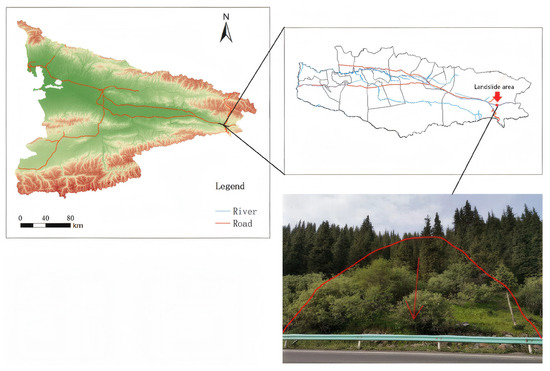
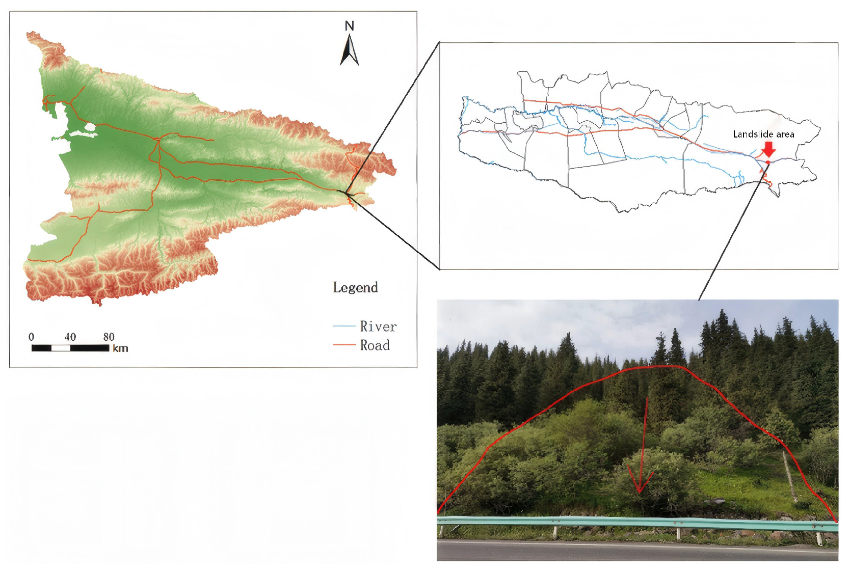
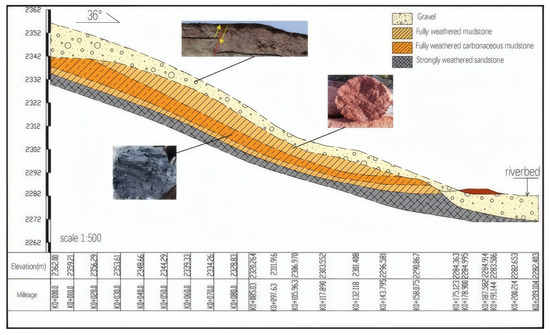
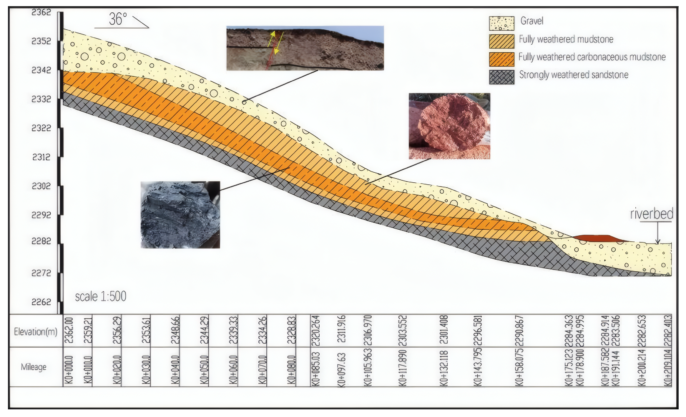
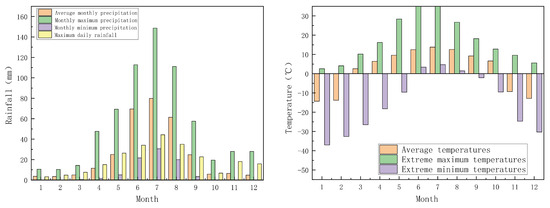
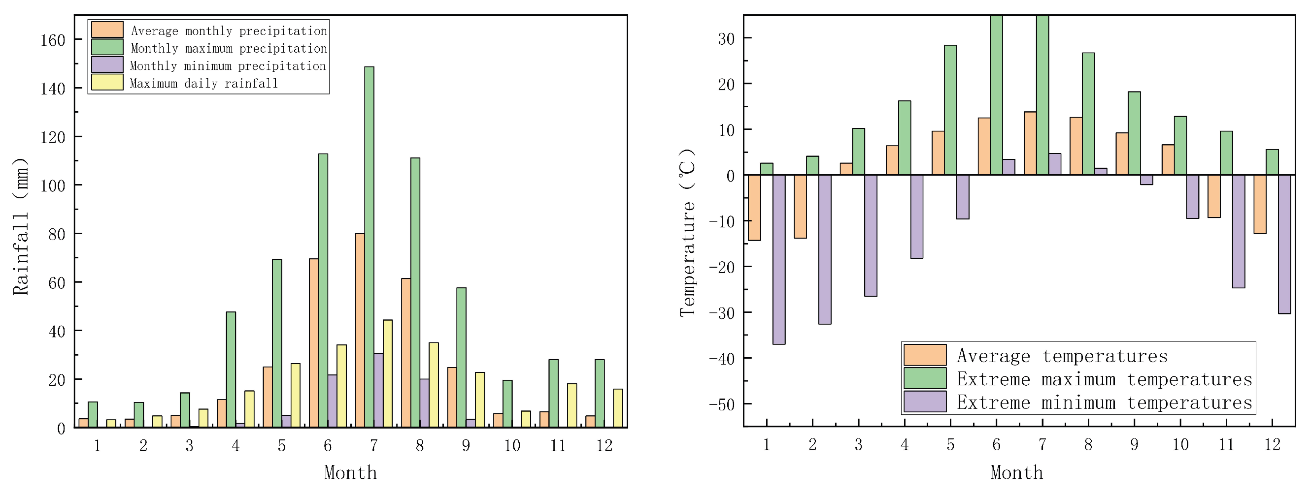
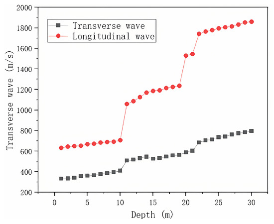
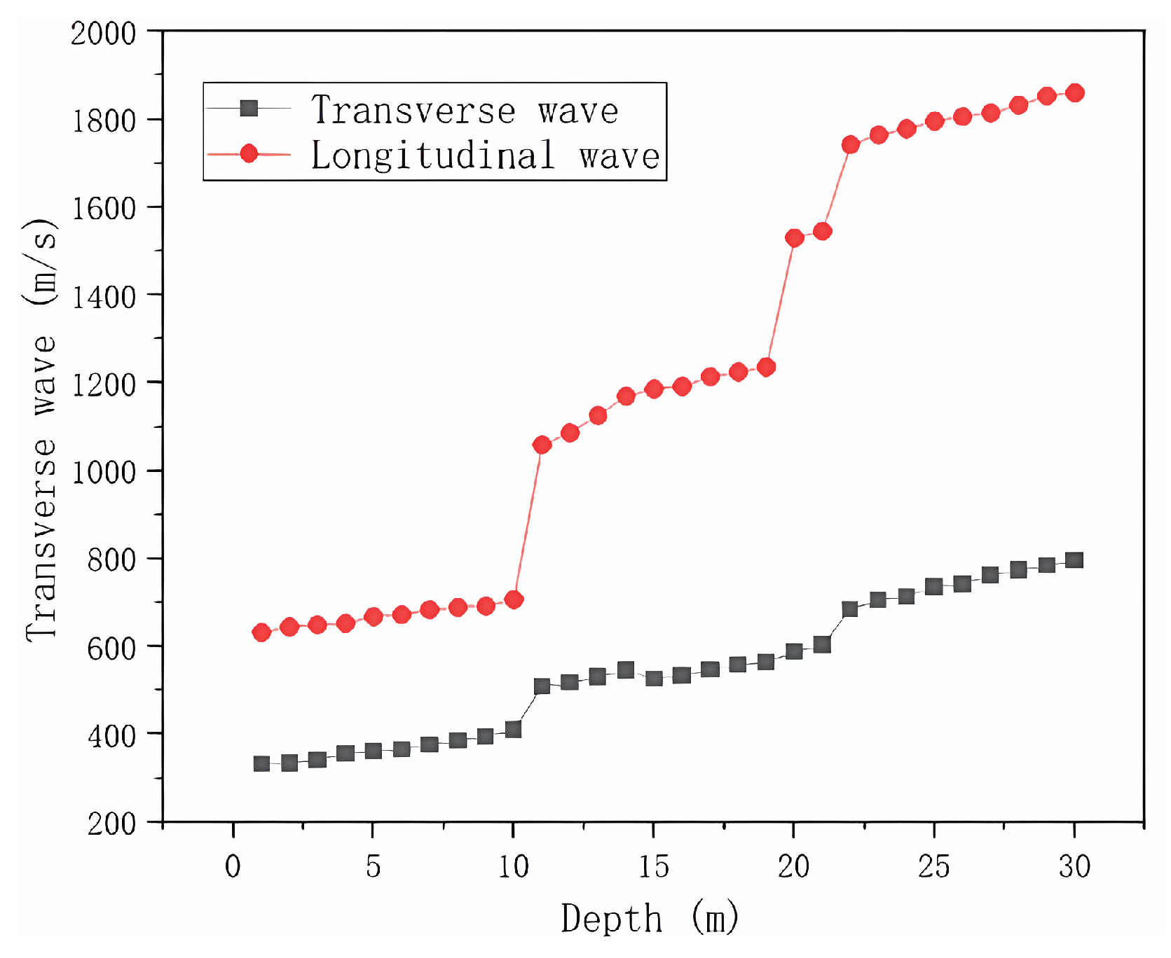
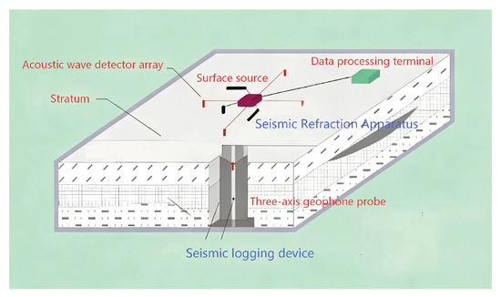
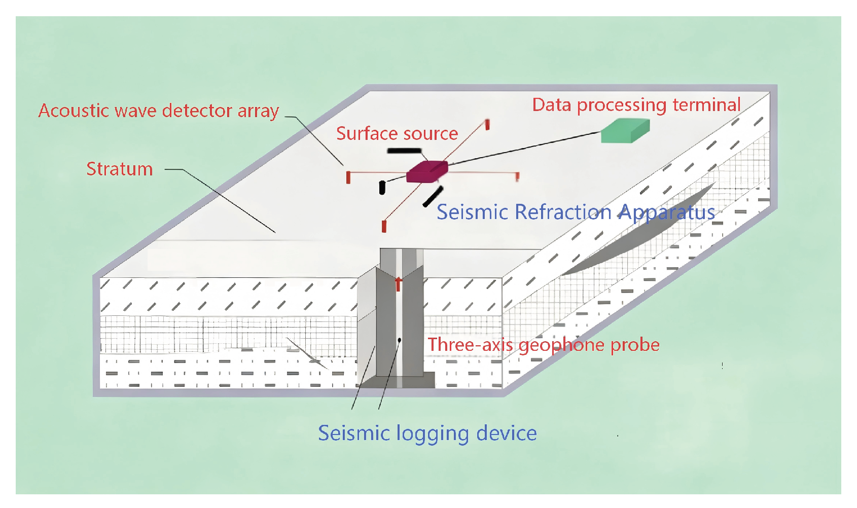
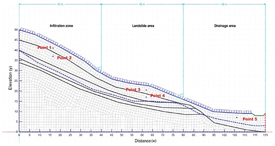
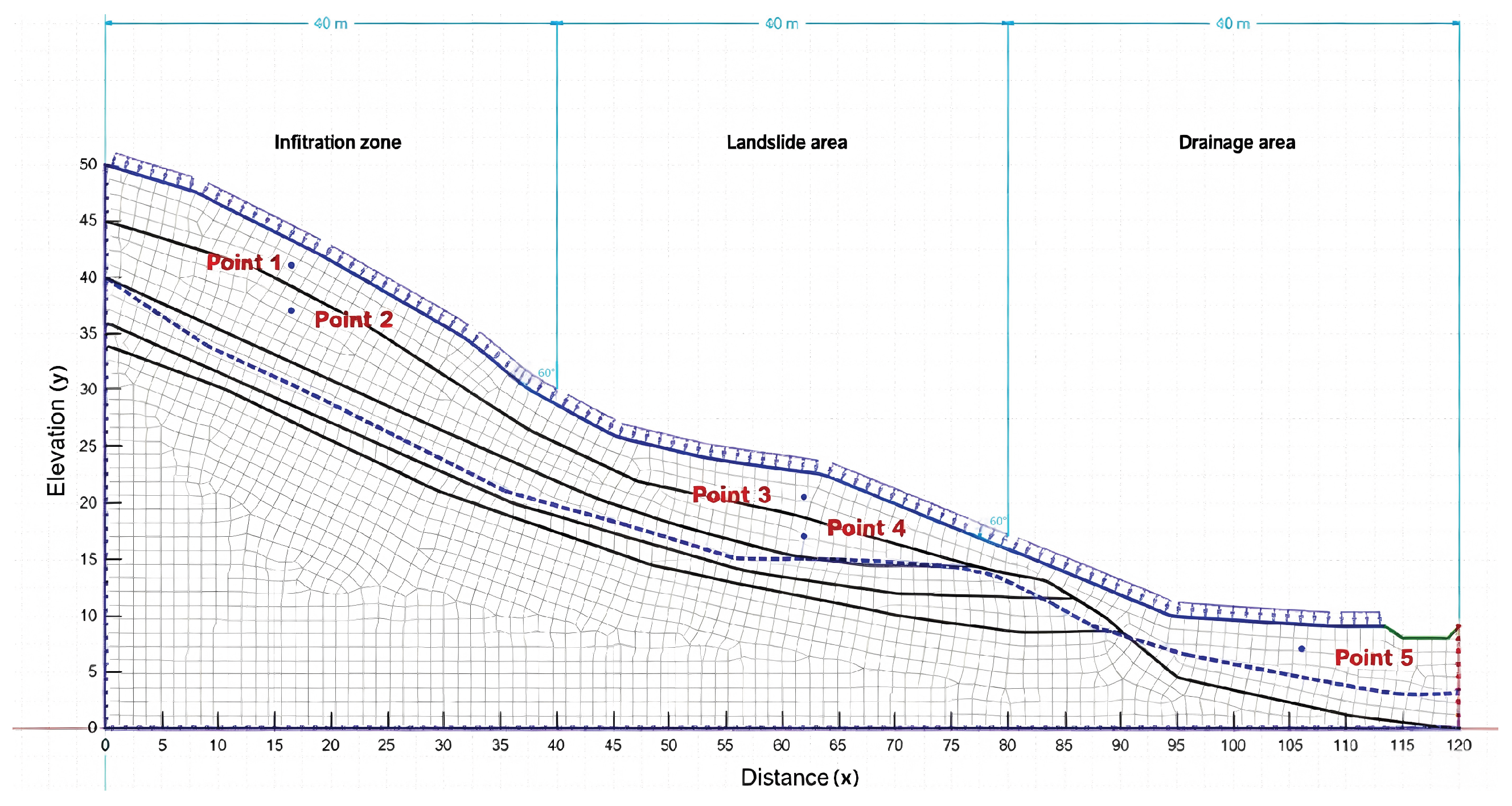
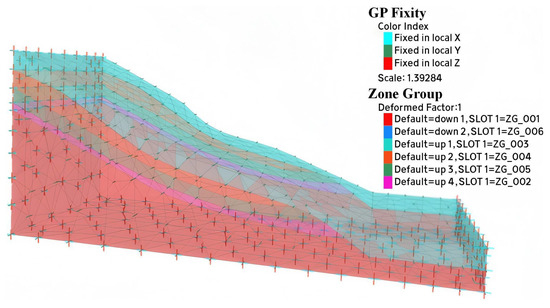
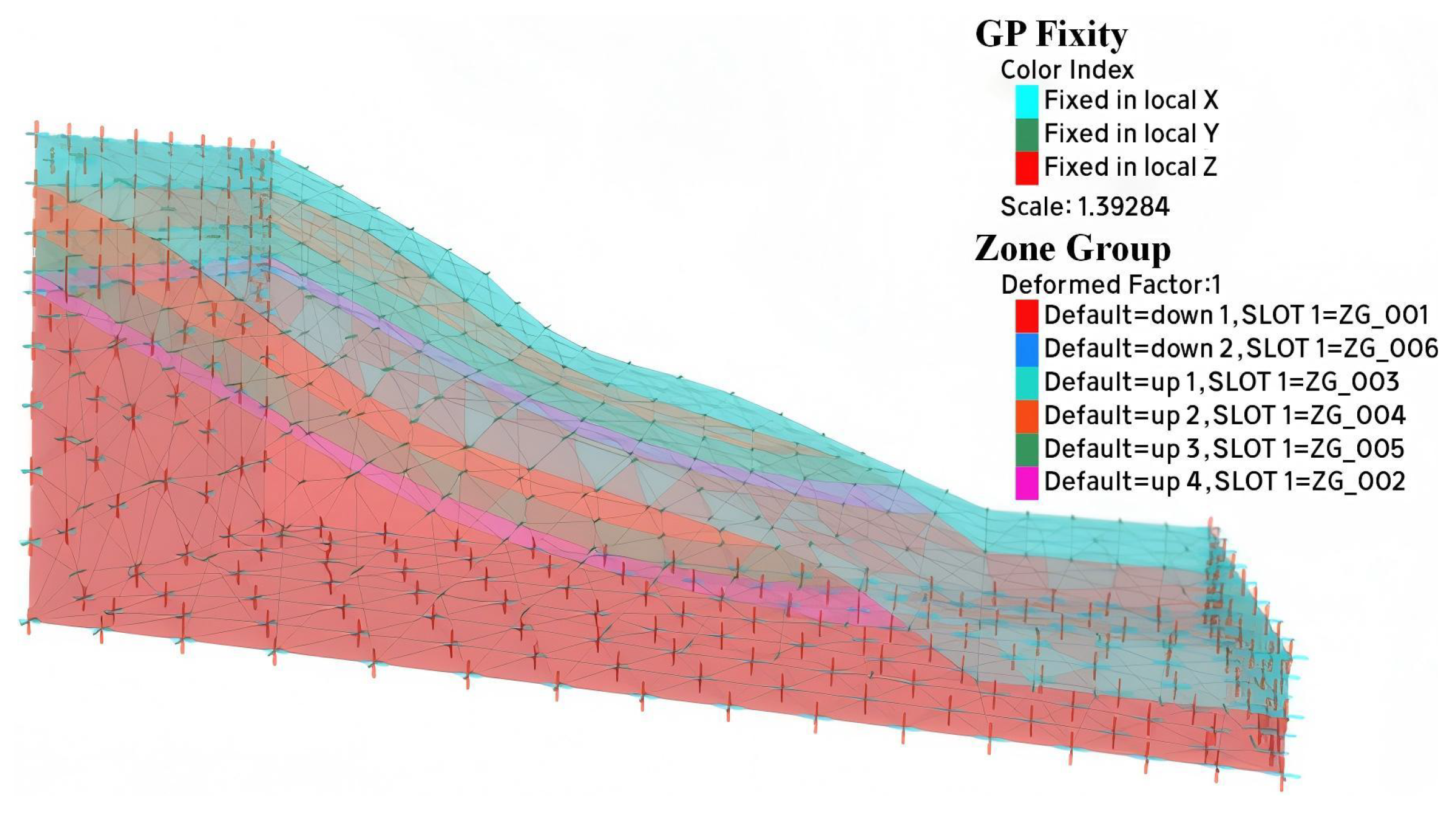
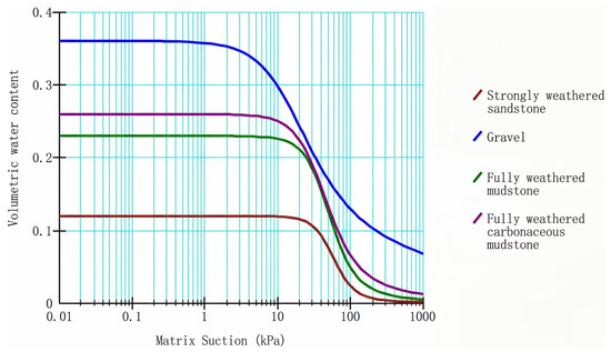
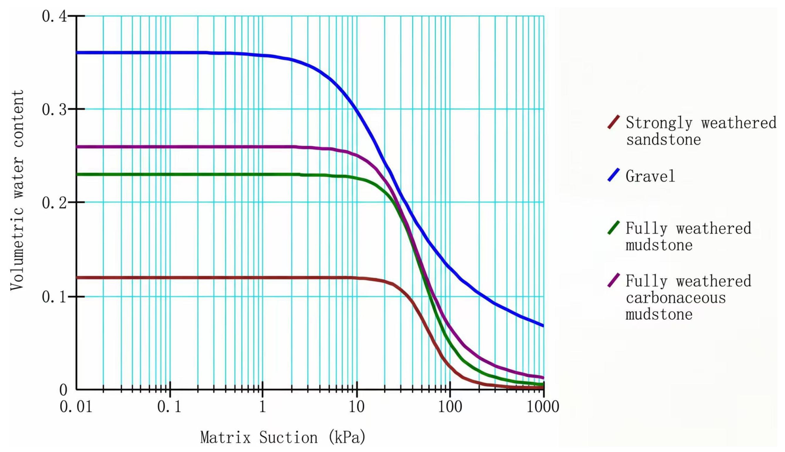
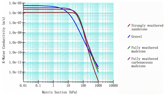
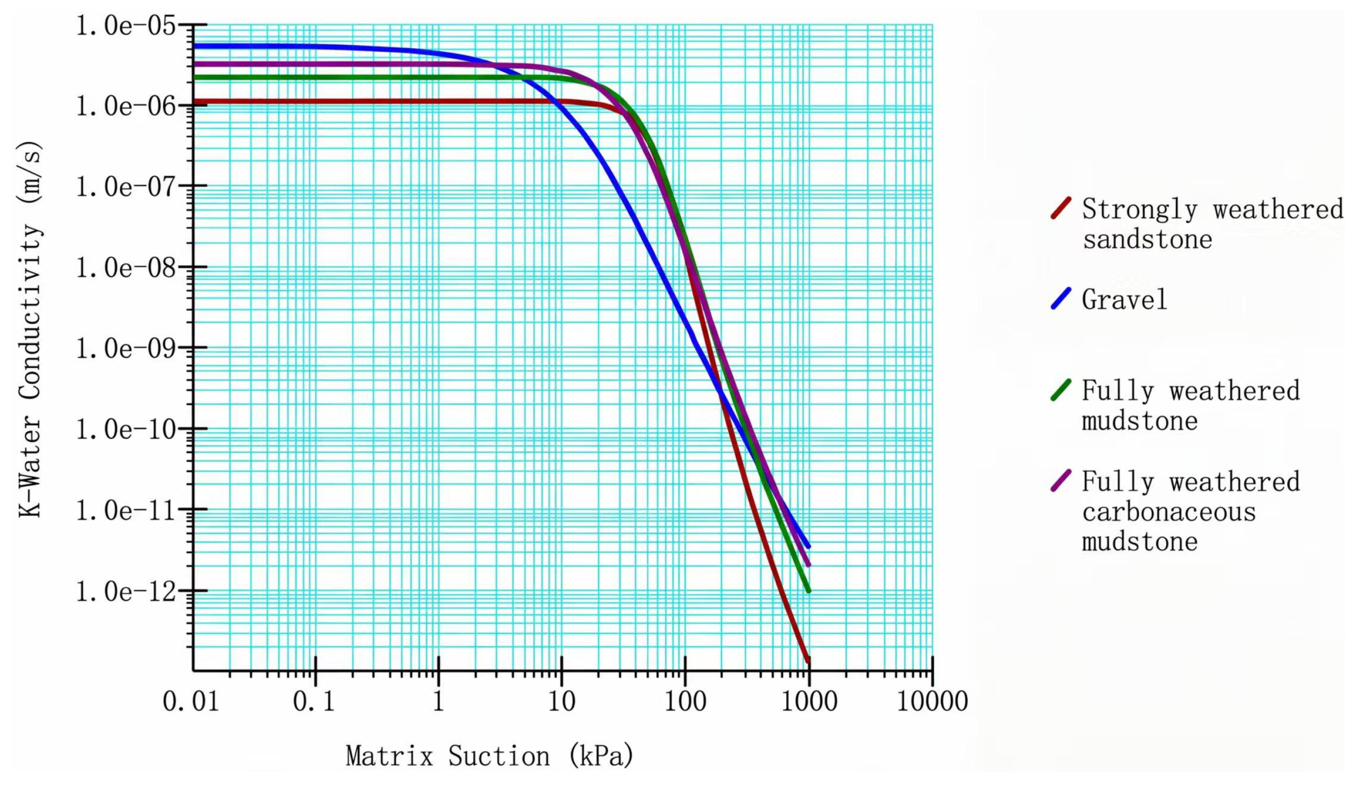
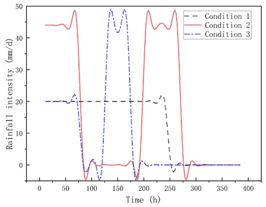
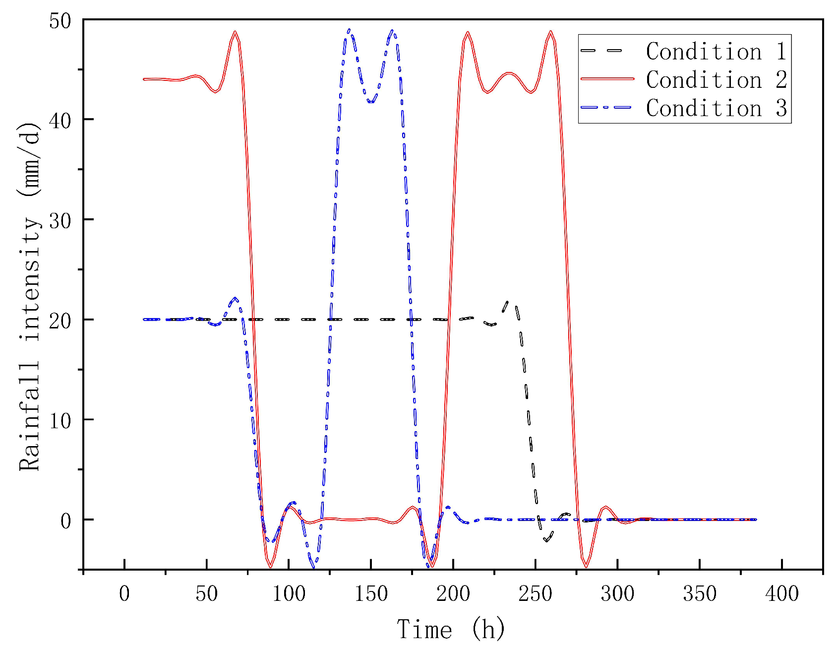
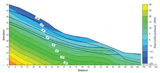
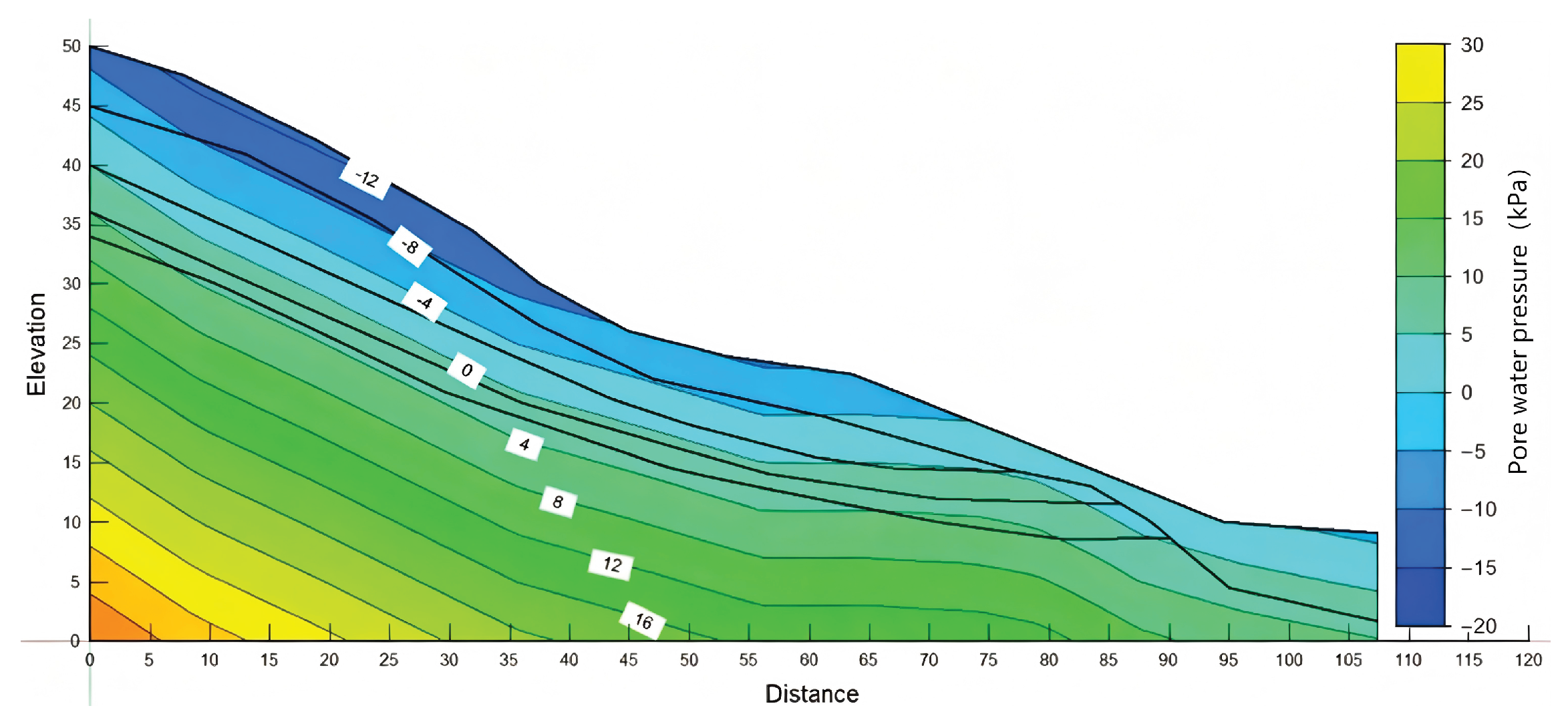
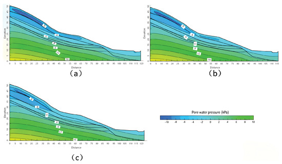
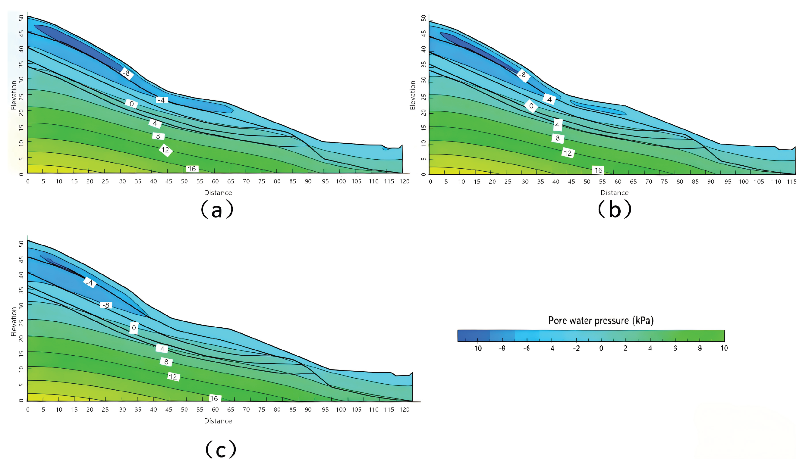
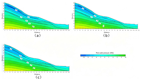
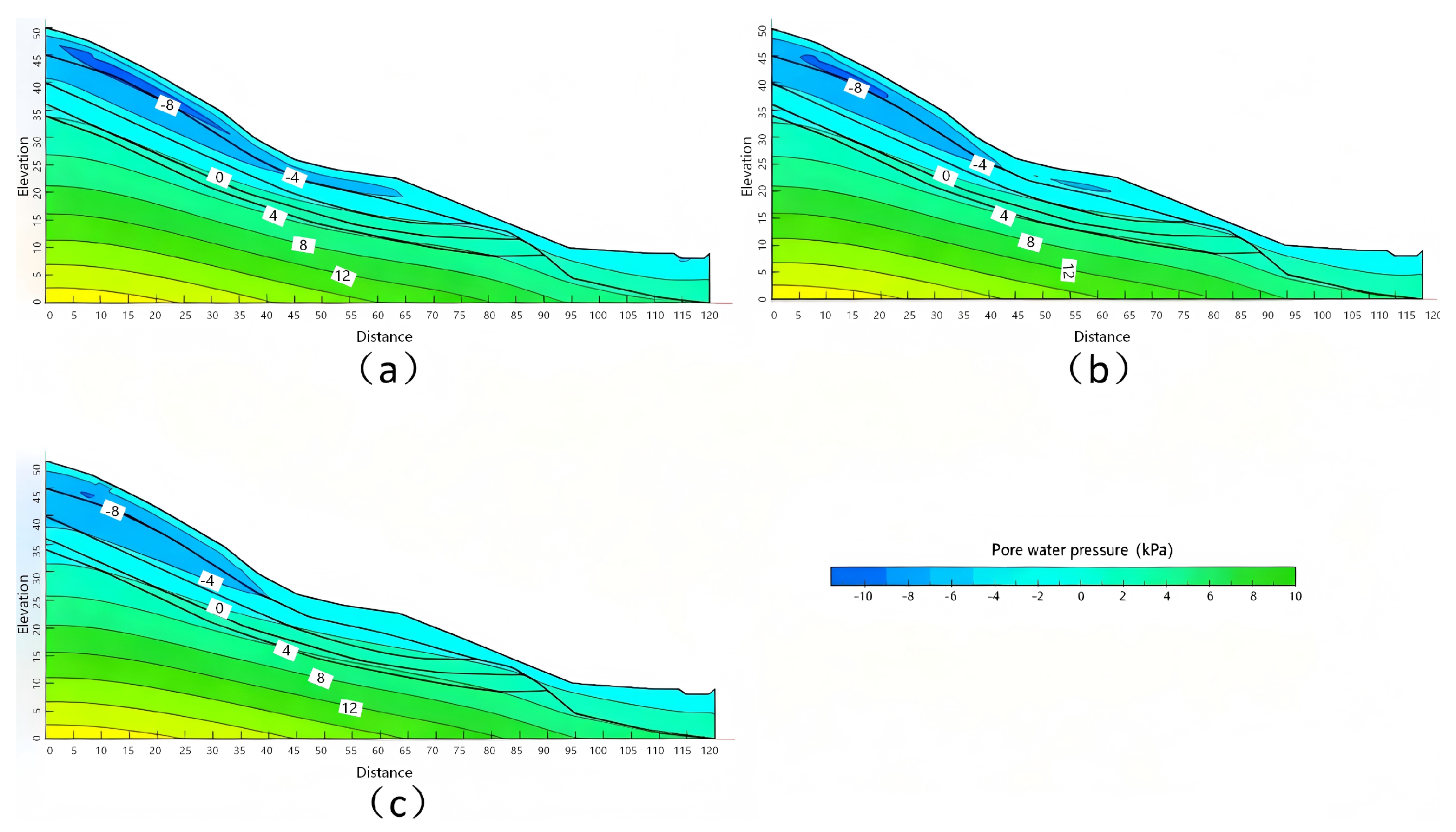
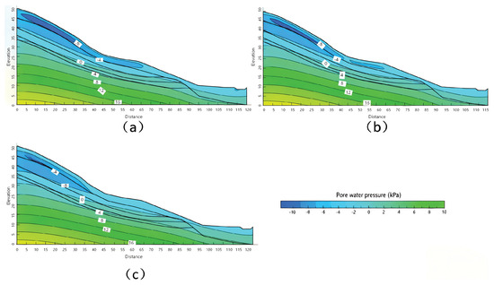
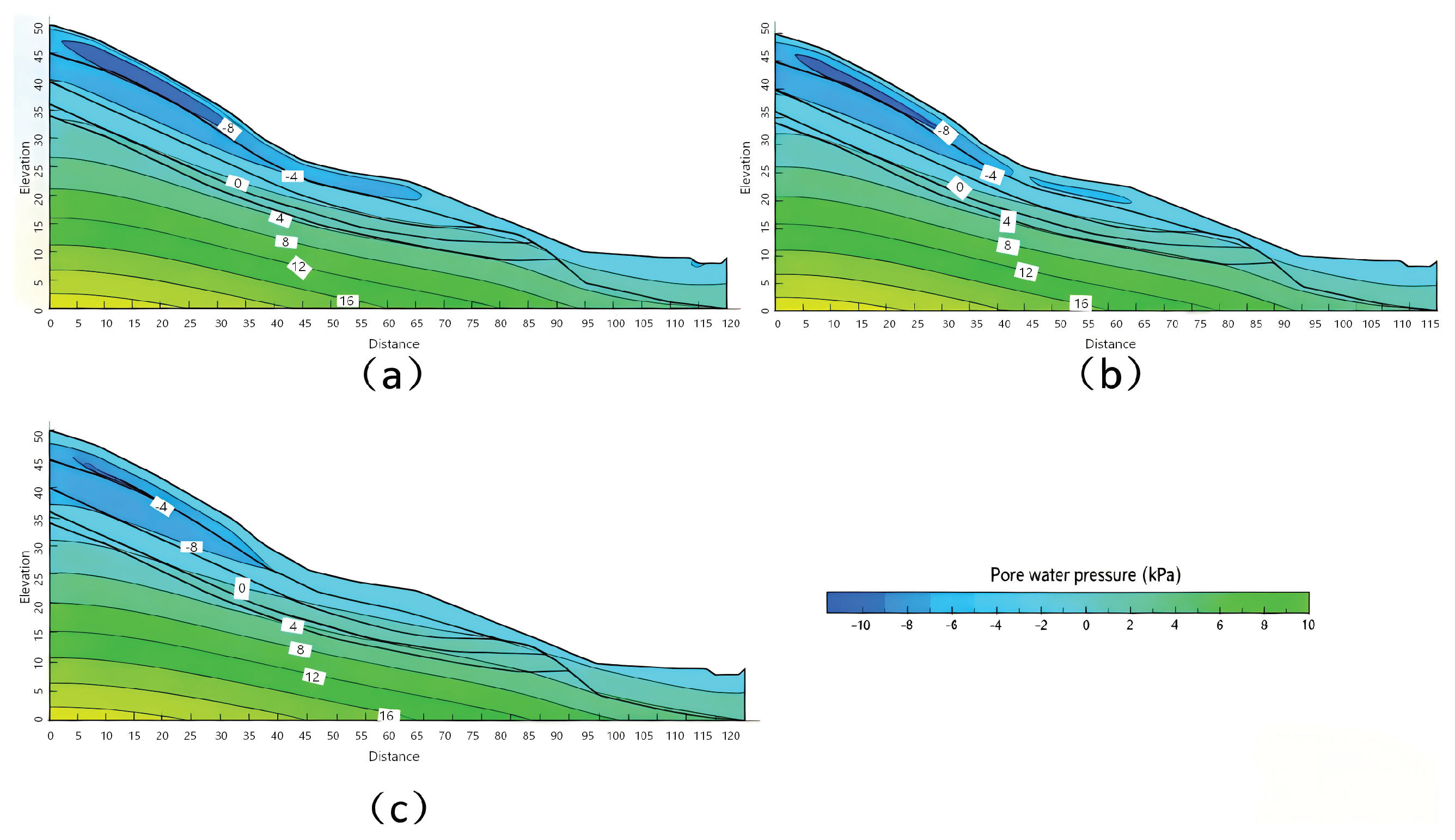
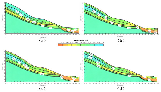
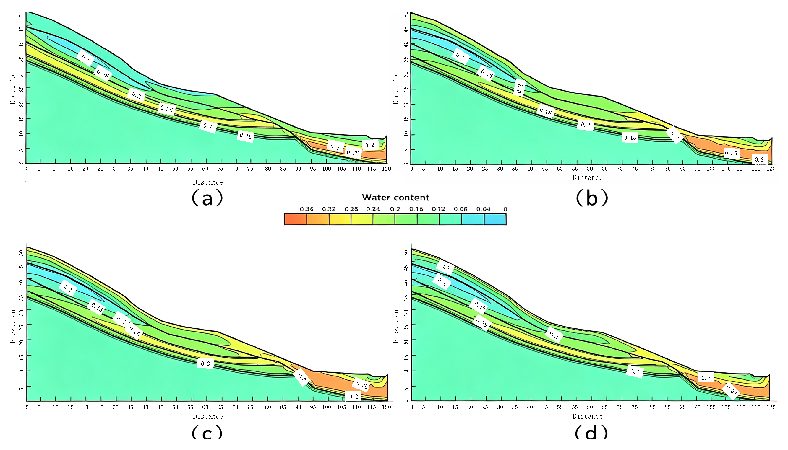
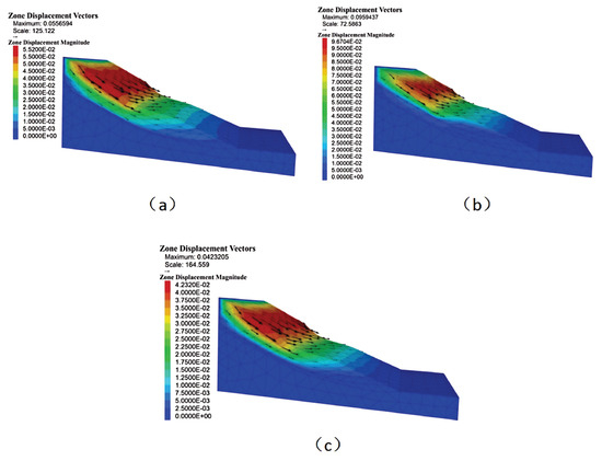
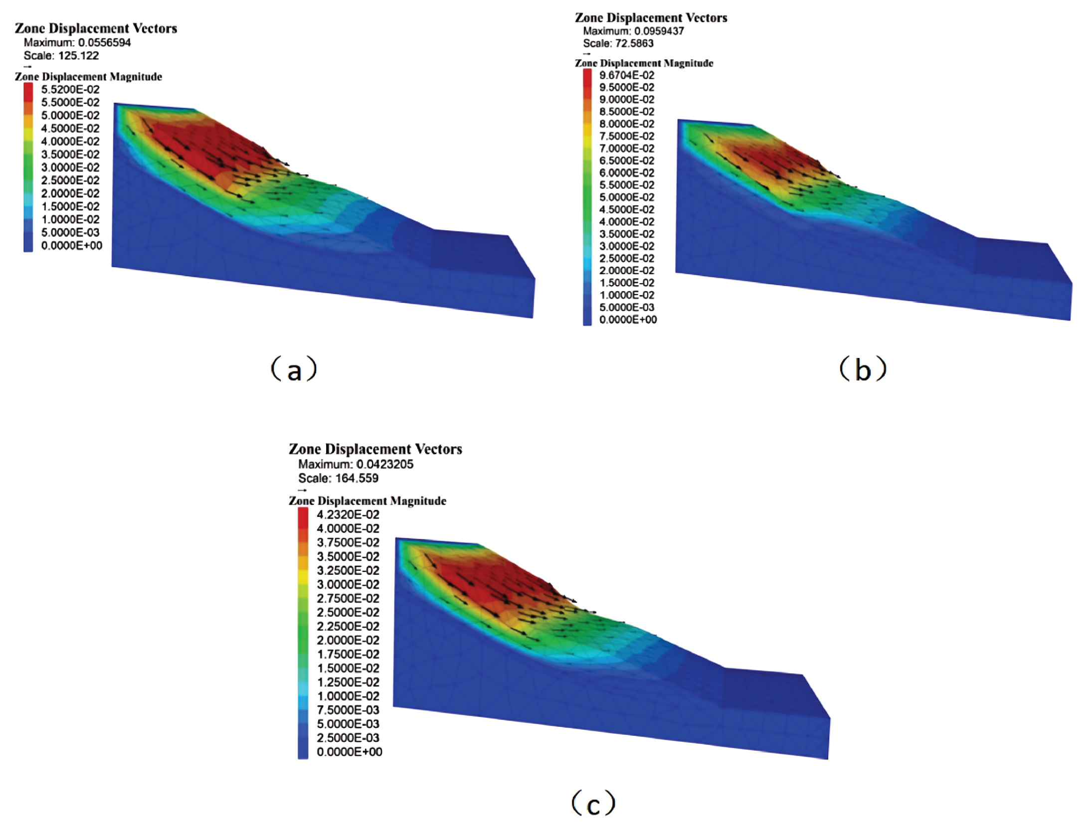
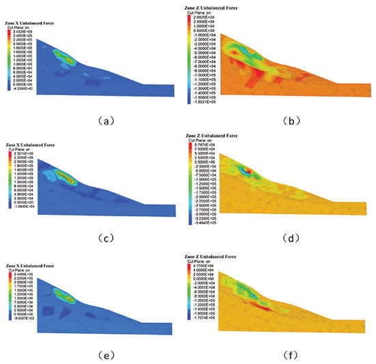
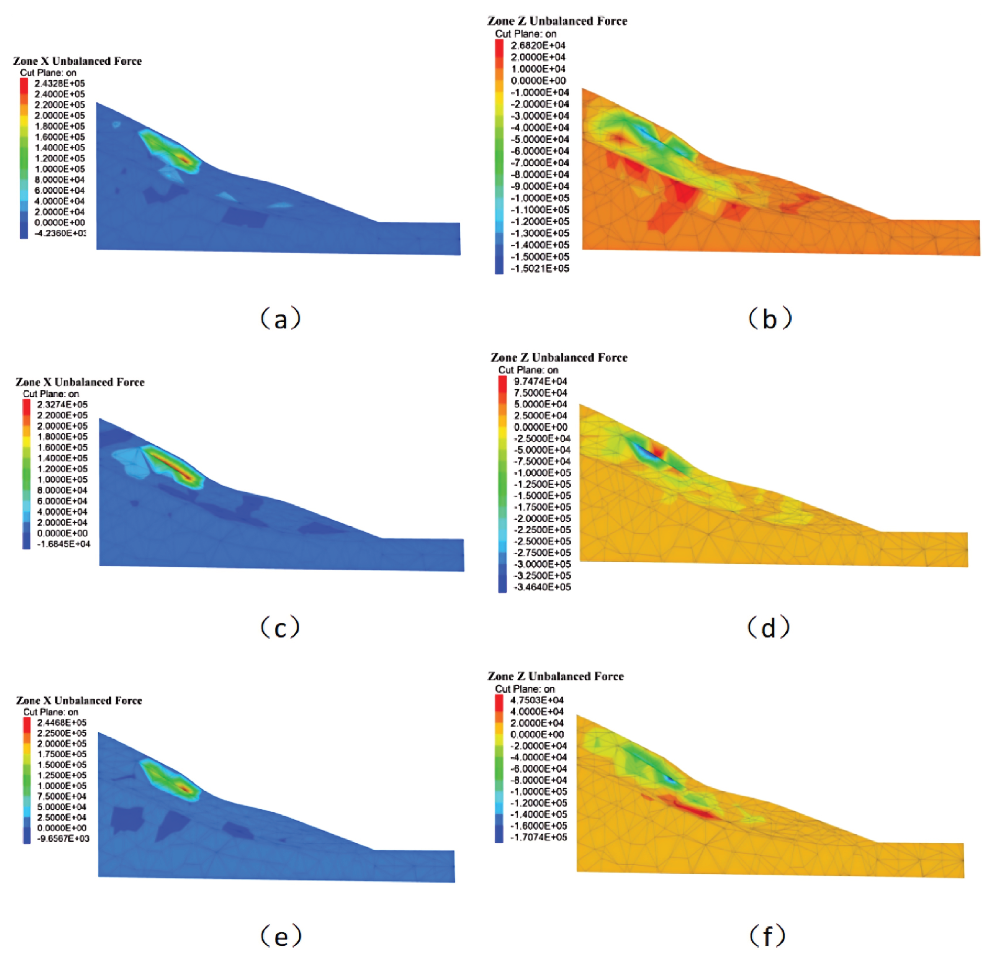
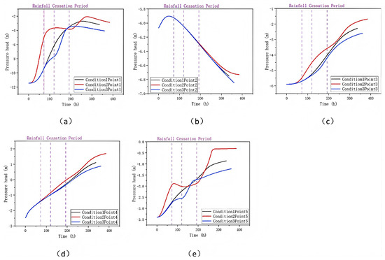
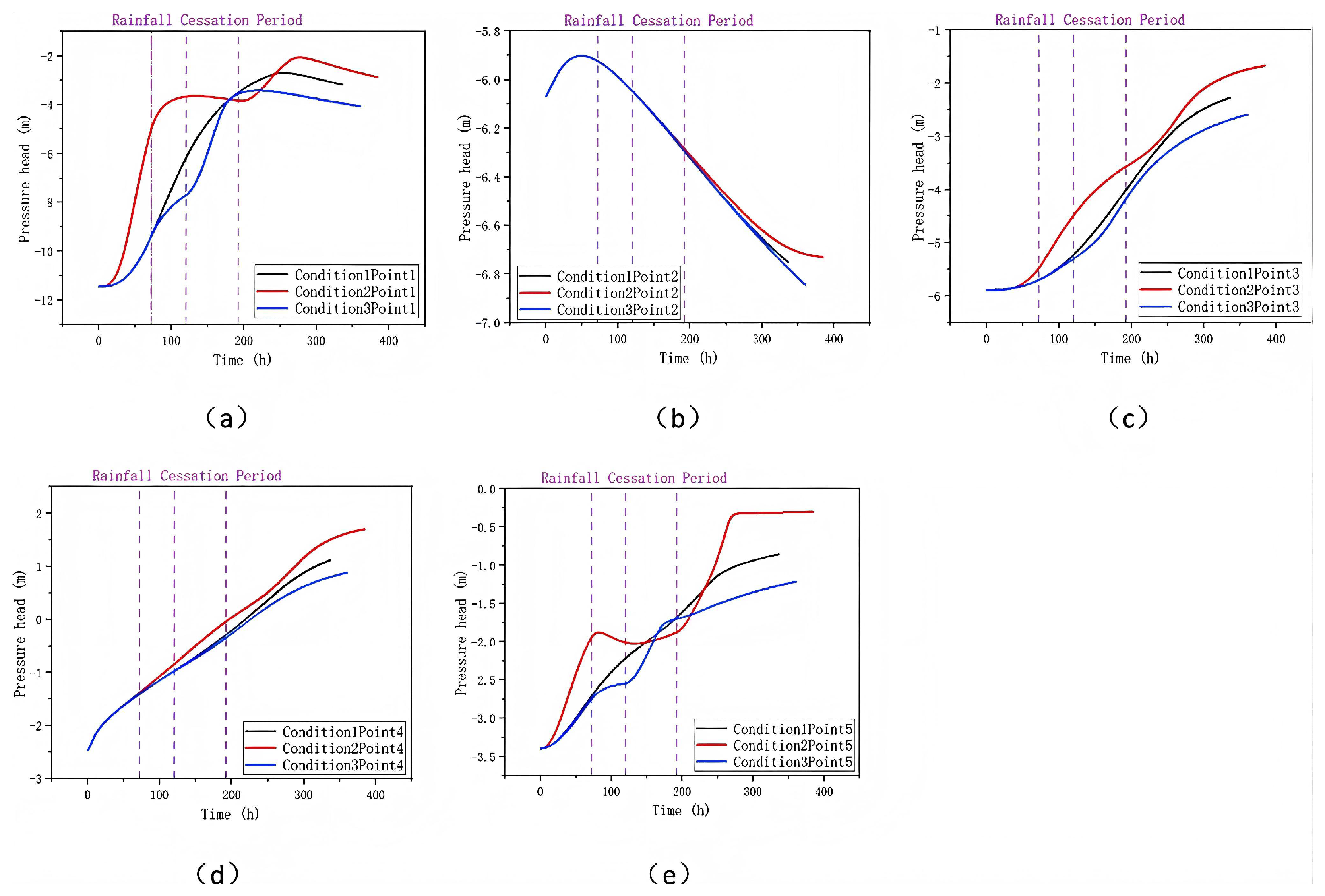
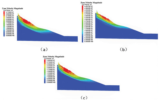
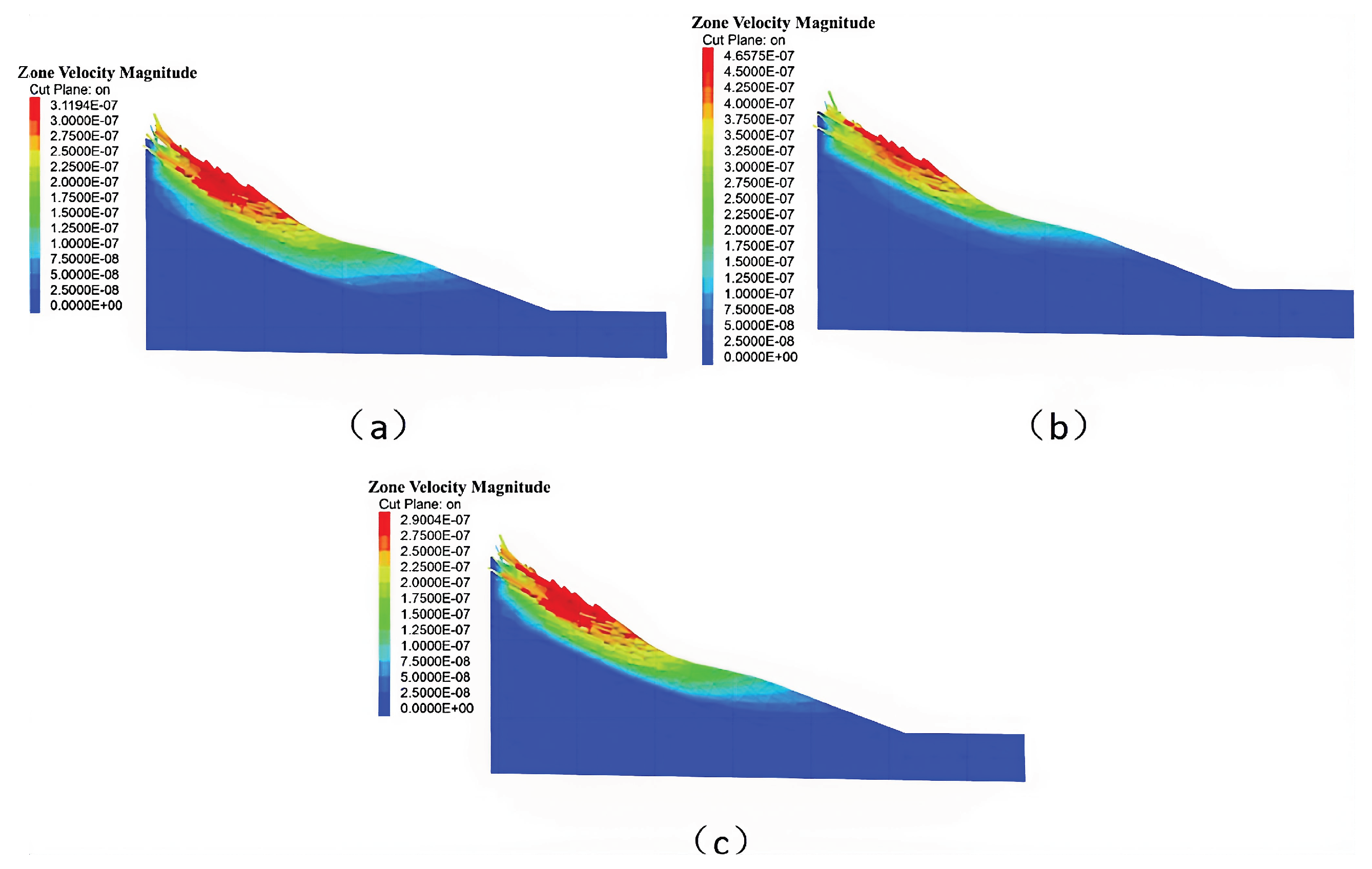
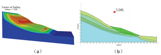
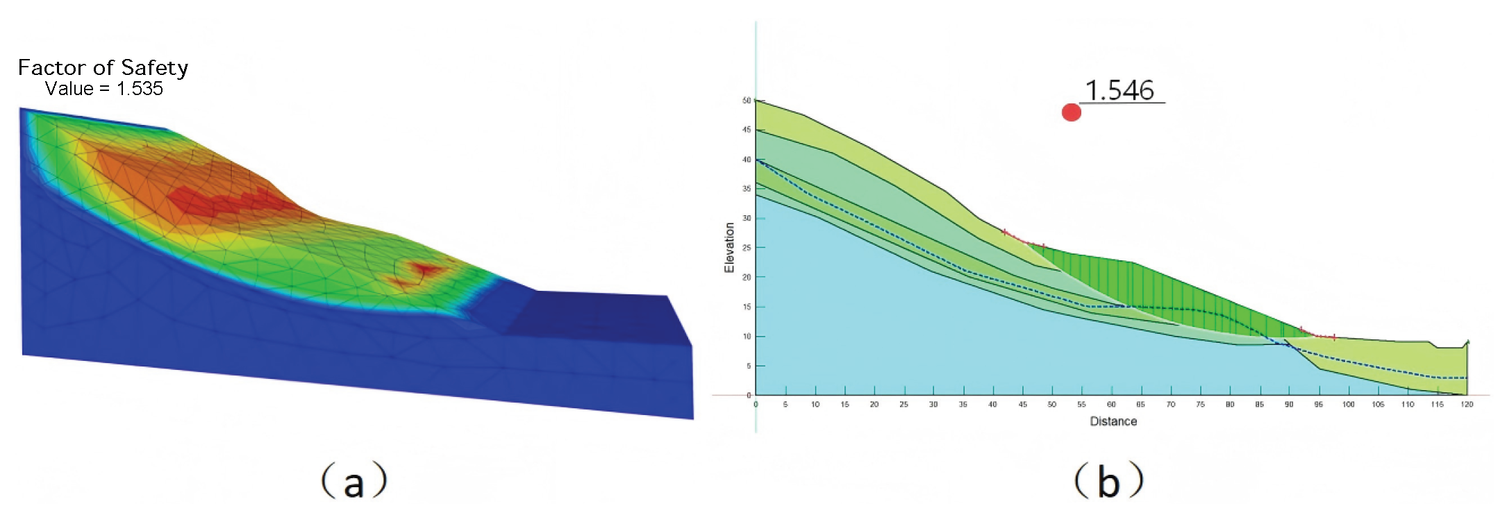
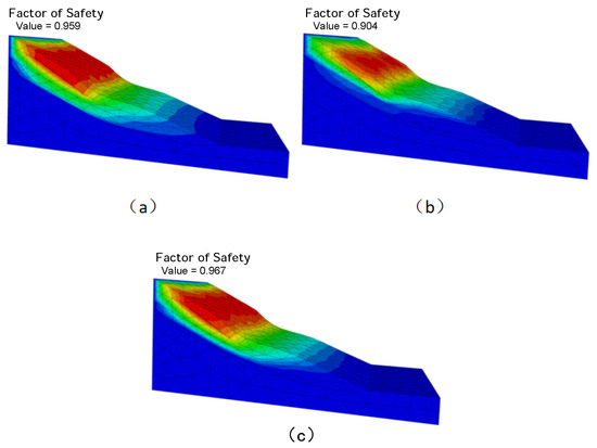
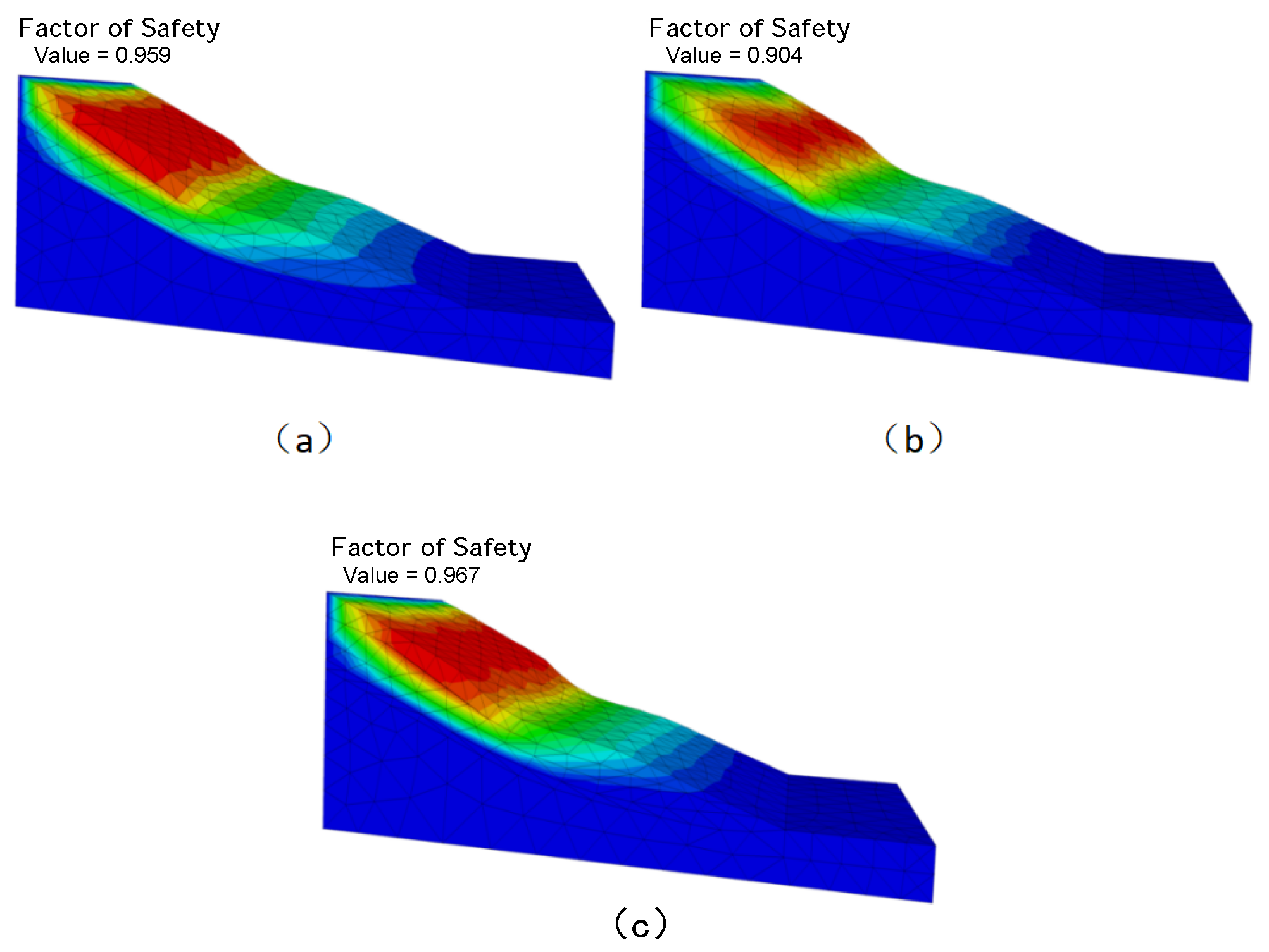
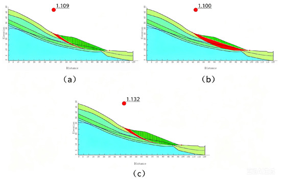
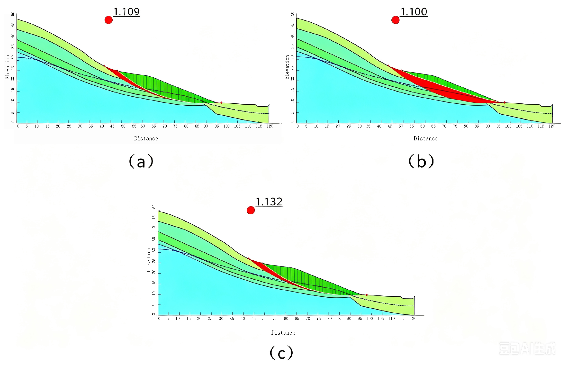
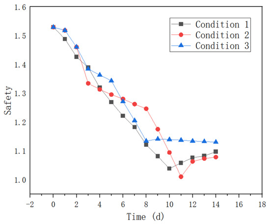
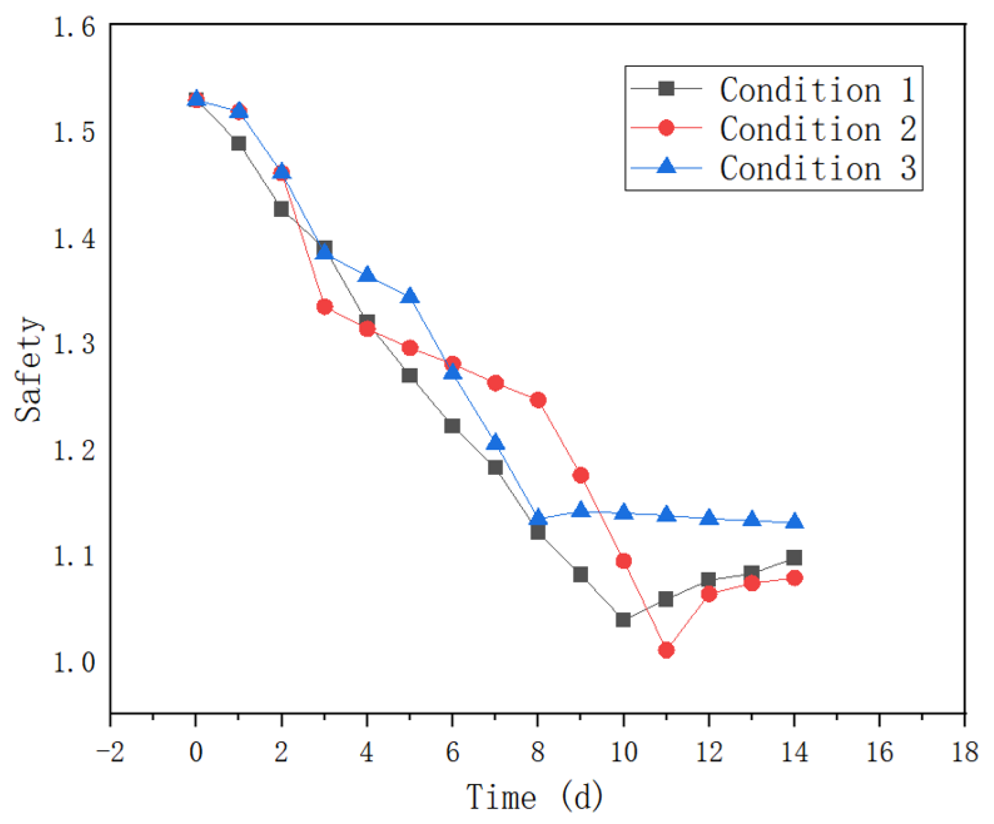

Disclaimer/Publisher’s Note: The statements, opinions and data contained in all publications are solely those of the individual author(s) and contributor(s) and not of MDPI and/or the editor(s). MDPI and/or the editor(s) disclaim responsibility for any injury to people or property resulting from any ideas, methods, instructions or products referred to in the content. |
© 2026 by the authors. Licensee MDPI, Basel, Switzerland. This article is an open access article distributed under the terms and conditions of the Creative Commons Attribution (CC BY) license.