


Abstract
Modelling and prediction of mean monthly flow are of particular importance for long-term planning in hydrology and water resources management. Therefore, a simplified and robust modelling procedure, derived from clearly and concisely established methodology, can benefit both researchers and practitioners. The main objective of this study is to develop a robust yet simple model, capable of producing predictions of satisfactory accuracy on previously unseen data. Two chronological data allocation strategies (C1 and C2), differing in the proportions of training, calibration, and verification subsets, were evaluated to analyze their influence on model accuracy and reliability. Chain and ensemble modelling techniques were applied, resulting in several stacking regressors with different combinations of base models and final estimators. The best-performing ensemble (C2) consisted of a support vector machine, histogram gradient boosting regressor, elastic net, and two dummy regressors as base models, with an artificial neural network as the final estimator. Within the ensemble structure, dummy regressors and histogram gradient boosting regressor were used to extend the predictive range, while elastic net and support vector machine captured the overall flow bias and fundamental flow dynamics. The artificial neural network final estimator was used to integrate these components into the final flow prediction. Compared to C1, the C2 allocations strategy achieved improved generalization capability and narrower confidence intervals due to the larger training subset, indicating higher model reliability for long-term monthly flow forecasting. The study additionally emphasizes the importance of appropriate methodological workflow, careful dataset treatment, and comprehensive model evaluation using complementary statistical and hydrological analysis tools.
1. Introduction
As supervised learning models rely heavily on the structure of the data, the choice and calibration of an appropriate mathematical model can be challenging. From the perspective of hydrological modelling paradigms, supervised learning belongs to the group of data-driven approaches, in contrast to physically based and conceptual hydrological models [1,2,3,4]. Rather than explicitly describing hydrological processes, supervised learning models derive relationships directly from patterns in observational data [4]. Such approaches may be particularly suitable for hydrologically complex systems, where physical process representation remains complex or uncertain, provided that sufficient data are available [2,3,4]. In karst catchments such as the Cetina River basin in Croatia, belonging to the Dinaric karst region, where groundwater flows are highly heterogeneous and hydrologically complex [5], data-driven approaches may provide a practical alternative to explicit physical process representation. In contrast to many traditional regression-based statistical approaches, machine learning, that is, supervised learning, offers greater flexibility in representing complex and nonlinear relationships [3,4,6]. However, model performance remains strongly dependent on the quantity and quality of available data, while physical interpretability is generally lower than in process-based hydrological models [1,2]. Modelling procedures, specifically the creation of models, vary considerably across different studies, while the number and diversity of machine learning approaches applied in hydrology have increased substantially over the last two decades [1,3,7]. A general tendency towards the development of increasingly complex machine learning models, often motivated by improvement in predictive performance, can also be observed in the recent literature [7,8]. In hydrology, the temporal framework of prediction (forecasting) can be classified as real-time, short-term, mid-term and long-term [9]. Since supervised learning models depend on both the data structure and dataset length, different frameworks lead to a wide range of modelling procedures. Different supervised learning models may perform differently depending on dataset size, structure, and problem formulation, while the amount of available training data may substantially influence predictive capability and model robustness (e.g., [1,10,11,12,13]). However, the abundance of different models has led many studies to focus primarily on finding a niche in developing new, more complex models, often inadvertently neglecting the importance of the modelling steps preceding and succeeding the model selection and creation [3,14]. During development of this study and review of the related literature, several methodological challenges relevant to supervised learning in hydrology were identified, generally consistent with concerns regarding data treatment, information leakage, model evaluation and performance assessment previously discussed by other authors [3,14]. First, the initial steps of model creation—including dataset preparation, inspection, splitting, analysis and treatment—are often briefly described, aggravating reproducibility and interpretation of results. Since supervised learning models are strongly data-driven, careful treatment of data prior to model evaluation is essential. Second, many studies rely on training and calibration subsets, while independent verification on previously unseen data is less frequently emphasized. Third, comprehensive model evaluation using both statistical indicators and traditional hydrological analysis tools (such as duration curves and hydrological-year assessment) is rarely systematically presented. Finally, increasing model complexity is often prioritized, while methodological transparency, uncertainty assessment, and practical applicability may receive less attention. These observations motivated the methodological framework proposed in this study. The proposed workflow does not represent a fundamentally new methodology, but rather an attempt to organize and apply procedures that appeared most appropriate and consistent with the observations and experiences gathered through literature review and model development.
Since we believe the models should serve practical purposes, we expect that at some point supervised learning models will be applied for long-term planning. However, neither a “best” nor a “perfect” model exists, and overoptimistic accuracy estimates can create a misleading perception of model reliability. Rather than focusing solely on performance metrics across different error measures or comparison with previously developed models, the intention of this study is to achieve a clearer and more structured understanding of model behaviour and realistic forecasting capability. In the authors’ perspective, models in hydrology should be interpreted not only through point accuracy, but also through reliability and predictive uncertainty, similarly to the reliability-oriented interpretation commonly adopted in civil engineering design. Such perspectives are supported through uncertainty-oriented and quantile-based approaches in contemporary hydrological forecasting studies [15,16]. Another common issue, particularly when only a small amount of data is available for training (since longer temporal frameworks result in fewer training data), is the modelling of low and high flows. Supervised learning models tend to more accurately predict flows that occur most frequently, while extreme low or high flows are often more difficult to reproduce reliably (e.g., [14,15,16]). In this work, the aim is to improve the accuracy of low and high flows through a simple combination of base models in the creation of an ensemble model. Accordingly, we propose splitting the modelling procedure into six clear and distinct steps: 1. Dataset preparation, inspection and split, 2. Data analysis and treatment, 3. Feature selection, 4. Model selection, 5. Optimization of model hyperparameters and selection of the final model, and 6. Model evaluation. To additionally investigate the influence of dataset allocation on predictive performance and reliability, two chronological dataset allocation strategies were introduced. The first approach (C1) uses a smaller training and calibration subset with a larger verification subset, while the second one (C2) allocates a larger portion of data for training and calibration. The intention was not only to compare point prediction accuracy, but also to evaluate how the amount of available training data influences model reliability and generalization capability under long-term forecasting conditions. The full set of tables and analysis providing insight into the model is given in the Supplementary Materials, almost in the form of a technical report.
The aim of this study is to develop a model for long-term forecasting of monthly flows at the Vinalić hydrological station on the Cetina River, Croatia. Additional objectives of this study are to: 1. Improve and emphasize the overall prediction modelling procedure by focusing on the complete methodology rather than isolated steps, while still providing a detailed description of each step through analysis and supporting figures. 2. Identify an appropriate approach for treating hydrological datasets in supervised learning by interpreting the influence of different models on prediction quality, and 3. Enhance the presentation of model evaluation (verification) by using associated tools (analysis, tables, figures) that provide insight into model behaviour and expected performance. The main contribution of the study is therefore not the development of an entirely new supervised learning algorithm or methodological novelty, but rather the transparent methodological integration, systematic evaluation and reliability-oriented interpretation of supervised learning approaches—including the proposed stacking regressor configuration combining quantile-based dummy regressors, support vector machine, histogram gradient boosting regressor, elastic net and artificial neural network.
The hypotheses of this work are as follows: 1. Ensemble modelling, using an appropriate combination of base models, can improve model performance in predicting low and high flows. 2. Dataset splitting affects not only model accuracy, but also model reliability, with larger amounts of training data generally leading to higher reliability. 3. If model evaluation is not entirely supported by associated tools (tables and figures showing averaged mean monthly flow, duration curves, confidence intervals of prediction), model performance may be misinterpreted.
2. State of the Art
2.1. Literature Review
This section provides a comparative overview of studies applying different numerical models that inspired the development and refinement of the models presented in the paper, focusing on model types, input data, evaluation approaches, and usage of exogenous and endogenous inputs. The comparison framework and structure of Table 1 are informed by existing syntheses available in the Open Research Knowledge Graph [17,18].
Table 1.
Overview of predictors, data transformation, tuning, performance and model evaluation.
The discussion begins with studies that use exclusively endogenous input data. The earliest and perhaps the simplest among the examined studies is [19], which develops models for the prediction of monthly flow on two rivers and compares the accuracy of SVM and its combination with discrete wavelet transformation. An SVM trained with antecedent 1–3 flows as inputs is compared with an SVM trained with 1–3 antecedent wavelet decompositions of flows. Based on flow data, ref. [20] investigate the potential of the ELM method for monthly flow forecasting and compare its performance with that of SVM and GRNN. For the ELM model, the number of neurons in a single hidden layer was optimized to minimize root mean squared error (RMSE) on the training dataset, while grid search and kernel spread optimization were applied for the SWM and GRNN models. To further improve the prediction accuracy using modified empirical mode decomposition M-EMD, ref. [21] compares the performance of ANN, SVM, EMD-SVM, M-EMD-SVM, and WT-SVM models. M-EMD was employed to eliminate end effects in the decomposition process. In [22], an improved SVM model with adaptive insensitive factors (LAIF-SVM and NAIF-SVM) is proposed. The chaos theory and phase-space reconstruction are introduced to overcome the empirical judgement of the structure of the forecasting model, while an improved PSO is applied to optimize model parameters. The case study results indicate that the proposed SVM variants enhance the generalization ability of conventional SVM models and improve prediction accuracy.
Given that models using exogenous inputs are suitable for the potential application of climatological model outputs, it is logical to continue the review in this direction. Accordingly, studies that do not use data transformation are discussed first (Table 1).
In [23], a model for monthly flow prediction is developed that explicitly accounts for spatial variability in hydrological processes. The main objective is to develop an integrated ANN model (IANN) composed of several individual ANN models, each representing a tributary, and to compare its performance with that of a lumped ANN (LANN), consisting of two ANNs representing upstream and downstream conditions. Data from stations and a digital elevation model were used to interpolate monthly precipitation and evapotranspiration over the basin and to later find average values for each tributary. The IANN imitates spatial heterogeneity by assigning a separate ANN to each of five tributaries, with the outputs of tributary-level ANNs serving as inputs to a final ANN model at the basin outlet.
Furthermore, the introduction of data transformation may lead to improvement of model accuracies, as demonstrated through the application of principal component analysis (PCA) for input variable decomposition in SVM [27]. In [27], a model for monthly flow prediction is developed with the aim of comparing the performance of SVM using a large number of inputs with those using a reduced input set and subsequently comparing these results with ANN employing a reduced input set. An SVM model trained using 6 input variables (3 antecedent values) is compared to SVM using inputs selected by PCA (5 values) and to SVM with inputs selected by forward selection (6 values). These models are then compared with an ANN model using a PCA-selected input set. In [3], a novel modelling workflow is proposed to address common challenges and pitfalls in the application of machine learning to hydrology. The workflow is applied to different machine learning models: SVM, ANN, ELM, RBF, and MLR. The study applies the workflow to select the most suitable machine learning model, compare it with MLR, assess the influence of PCA on performance, identify key predictors, and analyze the prediction performance for increasing lead times. In [28], streamflow time series are modelled using a feedforward MLP model tested with different combinations of exogenous input datasets, while the study reports improved prediction accuracy through the application of wavelet decomposition prior to ANN modelling (Table 1). Some studies report negative effects of improper data decomposition (preprocessing) on model performance [3,14]. In particular, ref. [14] highlights that in many studies, decomposition is applied before splitting the dataset into training/calibration/verification subsets. Applying decomposition in this manner leads to information leakage, as future values are implicitly used during preprocessing, even though such information would not be available at the exact moment of forecasting in real-world applications. Ref. [14] investigates the impact of data decomposition on model performance in both hindcasting and forecasting of monthly flow. The study compares the performance of models with decomposed inputs DWT-ANN, EMD-ANN, SSA-ANN, DWT-ARMA, EMD-ARMA and SSA-ARMA to the original ANN and ARMA. In the hindcasting experiment, the time series is first decomposed using DWT, EMD or SSA and subsequently split into training and testing datasets. In contrast, in the forecasting experiment, the time series is first split into training and testing datasets, after which decomposition is applied only to the training subset. During testing, each new observation is appended sequentially, and the decomposition is recalculated, thereby avoiding information leakage from future values.
Finally, ensemble models are constructed by combining multiple independent models. In [29], the potential of two ensemble learning paradigms—bagging and stochastic gradient boosting is examined for improving the accuracy of monthly flow prediction. The study compares SVM, CART, BRT, and GBRT and examines improvements in CART performance achieved through bagging and boosting. CART is used as the base estimator for BRT and GBRT. In [30], ensemble techniques are applied to improve the prediction of monthly flow produced by three conceptual water balance models (Rao, Guo and WASMOD-M). The models are calibrated using a genetic algorithm, after which several multi-model ensemble approaches—MBEM, FUCEP, OK, BMA and WA—are employed to enhance performance and compared. ANN models trained using Levenberg–Marquardt (ANN-LM) and the firefly algorithm (ANN-FA) are developed, and their outputs are utilized as inputs for multi-model ensemble approaches (MM-ANN and MM-SVM) in [31]. The study [32] forecasts inflow to five hydropower plants by comparing several modelling approaches, including ARIMA, SARIMA, ELM, ESN, as well as ensemble methods based on bagging (ELM-B, ESN-B) and multi-objective optimization (ELM-MOB, ESN-MOB). A unique contribution is presented in [33], which focuses on hindcasting missing monthly flow values using observations from neighbouring stations within the same region and develops a framework for selecting optimal features and a machine learning model for the purpose. A wide range of models is evaluated, most of which include AdaBoost and bagging regressors as base models of ensemble—RFR, GBR, ETR, HGBR, RFR (ABR), RFR (BR), GBR (ABR), GBR (BR), ETR (ABR), ETR (BR), HGBR (ABR), HGBR (BR). The emphasis of the study is on the modelling framework rather than fine-tuning individual models. The procedure is performed iteratively, first reconstructing missing values at the most correlated stations and subsequently refining accuracy by prioritizing stations with the poorest performance. Finally, research [34] pioneers the use of ECMWF runoff forecasts for monthly flow prediction, using MLR, ANN, SVR, RF, and XGBoost with repeated K-Fold cross-validation.
There are two basic types of ensemble models: (i) models that are ensemble-based by design—DTR, ETR, RFR, GBR, HGBR, XGBoost—which predominantly rely on decision trees as base learners; and (ii) ensemble wrappers that allow the user to combine different, arbitrarily selected base models—BR, AR, VR-voting regressor, SR-stacking regressor. Both types of ensemble models have been applied in various ways in hydrological predictions. For example, ref. [36] compares the performance of XGBoost with ANN, LSTM and RFR in predicting flow residuals from a physically based water balance model used for monthly flow prediction. Among the fore evaluated models, XGBoost achieved the highest accuracy. In [35], an improved stacking regression approach—stochastic weighted averaging combined with fold-wise weighted stacking—is proposed using three deep learning base models: LSTM, GRU and TCN. The proposed model outperformed individual base models, conventional stacking regression and standard stochastic weighted averaging. The authors report that stochastic weighted averaging enhances model generalization by bypassing overtrained solutions, particularly when combined with fold-wise weighted stacking. In this paper, the focus is placed on the selection of base models and their training in a way that enables effective representation of flow bias and variance through appropriately chosen base learners.
Finally, as models generally tend to underestimate peak flows (and sometimes overestimate low flows), table property peak flow determines whether model performance is evaluated on specific high-flow events. It is therefore particularly important to assess how models perform in the range of extreme and infrequently observed values. Within the reviewed studies summarized in Table 1, explicit peak-flow evaluation was included in a limited number of cases (e.g., [19,29]).
2.2. Conclusions from Literature Review
As already noted, the review is based on two comparative analyses [17,18]. The first aims to provide insight into applied methods and techniques, while the second offers a broader representation of approaches, in the form of a statistical sample of studies. Based on the overview of 20 contributions published between 2011 and 2023, several interesting conclusions can be drawn [18]. The literature shows a strong emphasis on developing increasingly complex models in pursuit of higher accuracy, often at the expense of appropriate methodology, rigorous model evaluation, and careful interpretation of results. In contrast, the main objective of this study is to develop a robust yet relatively simple model. Nevertheless, addressing the identified challenges required the adoption of a moderately complex modelling strategy. The most accurate model on the calibration subset—the stacking regressor—is constructed from previously developed base models, with their outputs serving as inputs to the final predictive model.
Data from observation stations are commonly used (in every paper), whereas outputs from other models (meteorological, climatological) are employed much less frequently, appearing in 3 out of 20 papers. As expected, the number of instances (data samples) and the length of the historical dataset vary considerably, typically spanning at least 18–20 years or more. However, these characteristics are largely determined by data availability and are generally beyond the authors’ control.
Forecasting horizons longer than one month are rarely considered (3 out of 19, without hindcasting), while hindcasting is addressed in just one study. Among the summarized studies, only 4 out of 19 (20) studies split the dataset into three subsets. For proper and fully independent evaluation of the model’s forecasting performance, assessment should be conducted on a dataset portion entirely unseen during model development, as this best represents the future conditions and preserves the leave-future-out principle recommended in time series forecasting literature [3,37,38]. However, it should be noted that for hindcasting (reconstruction of historical data), a three-way dataset split is not required, as the primary objective is not operational forecasting. Similarly, for the purpose of model intercomparison, a simple training-testing split may be sufficient. Nevertheless, for practical applications, it is essential to evaluate how the model truly performs under conditions that emulate real-world forecasting, where future data is completely unknown. Endogenous predictors are used in 15 out of 20 studies, while exogenous predictors appear in 13 out of 20. Simultaneous use of both predictor types is reported in 5 studies.
In 12 out of 20, the use of data scaling is not reported. For most supervised learning models, data scaling is a key prerequisite for achieving satisfactory performance. While it is reasonable to assume that scaling is often applied, it is frequently treated as a minor preprocessing step and therefore omitted from reporting. In 7 out of 20 studies, data decomposition or dimensionality reduction is applied. Feature selection is predominantly based on simple choices of antecedent values or correlation-based methods (16 out of 20 studies), while some form of automated feature selection is implemented in 4 studies. None of the reviewed studies employ models capable of predicting multiple outputs or chains; all focus on single-output prediction per instance. In relation to the first additional objective, the intention in this paper is to clearly describe all steps of the modelling procedure and the methodology as a whole. E.g. oversight at the very beginning of model development, such as improper dataset separation, could lead to errors at the later stages of the modelling process.
The most frequently applied models are artificial neural networks (12 studies) and support vector machine (9 studies), while other models are used less often—gradient boosting regressor (3), extreme learning machine (3), random forest regressor (2), extra trees regressor (1), AdaBoost regressor (1), and other newly developed models. In six studies, some form of ensemble model is employed. In 9 out of 20 studies, three or fewer models are examined, while 11 out of 20 deal with more than 3 different supervised learning models. In relation to the second additional objective, the performance of twelve (12) different models was evaluated for model C1, whereas five (5) models were examined for model C2, as the remaining models were considered unsuitable for this purpose. Five (5) stacking regressor combinations were evaluated for C1 and eleven (11) for C2.
Model evaluation is often insufficiently addressed, despite being essential for understanding the nature of model application in practice. It consists of three main components: performance metrics, visual comparison of observed and modelled values, and estimation of model uncertainty and reliability. Although model performance cannot be fully described by metrics alone, they provide valuable information for comparing model performance. It is somewhat expected that at least one commonly applied absolute metric (e.g., mean absolute error or root mean square error) and one relative metric (e.g., coefficient of determination or Nash-Sutcliffe efficiency) are reported due to their ease of interpretation. Graphical comparisons of observed and modelled values are commonly applied (16 out of 20 studies), as are observation-model comparison plots such as quantile-quantile plots (14 out of 20). In contrast, specific evaluation of peak flows is rarely conducted (3 out of 20), as is the assessment of model uncertainty (4 out of 20) and modelled yearly averages (1 out of 20). Similarly, modelled duration curves appear only occasionally in the literature (e.g., [39,40]). In relation to the third additional objective, the intention is to extract as much information as possible from the selected best-performing model in order to enable a valid interpretation of its results and realistic expectations of its practical performance.
3. Materials and Methods
3.1. Methodological Framework and Research Area
This chapter outlines the methodology applied for modelling mean monthly flow using supervised learning, following approaches from previous studies [41,42]. The workflow consists of six key steps noted in the Introduction as follows (Figure 1): steps 1–3 (dataset preparation, inspection, and split; Data analysis and treatment; Feature selection) are addressed in Section 3.2; steps 4–5 (model selection; optimization of model hyperparameters and final model selection) are addressed in Section 3.3; and step 6 (model evaluation) is addressed in Section 4 and Section 5 through results and discussion.
Figure 1.
Generalized methodological workflow applied for supervised learning modelling.
Figure 1 presents the generalized workflow of the supervised learning modelling procedure proposed in this paper. The workflow additionally distinguishes mandatory and optional modelling steps and emphasizes exclusion of the verification subset from preprocessing and optimization procedures in order to avoid information leakage. Exceptions are limited to procedures necessary for assigning previously defined variables, transformations, or scaling parameters obtained from the training and calibration subsets. Orange arrows distinguish the transfer of preprocessing parameters from the main workflow connections. They indicate that preprocessing is performed exclusively using the training, or training-calibration subsets, while the independent verification subset remains excluded, thereby preventing information leakage. The application of the workflow and its individual components is further clarified throughout the current methodological chapter. Although presented as separate workflow steps, model selection and hyperparameter optimization are closely interconnected and performed in an iterative feedback loop. Candidate models are first selected and subsequently optimized, after which their performance is reassessed, each time using the calibration subset. As demonstrated in this study, the hyperparameter optimization stage may also lead to the creation of additional ensemble models, which require further tuning and performance assessment before the final model is selected. The feedback arrows indicate that the workflow is not strictly linear and that previous steps, such as feature selection, may be revisited when necessary.
Two separate chronologically allocated input datasets (C1 and C2) were examined for training, calibration, and verification of the models using different subset proportions. The first (C1) allocates 40% of the available samples for training, 15% for calibration, and 45% for verification, while the second (C2) uses 60% for training and 20% each for calibration and verification. The two allocation strategies were introduced to evaluate the influence of training and verification subset proportions on model performance and generalization capability. All tables and figures for both procedures are provided in the Supplementary Materials, following the order of the modelling workflow. In the text, results are primarily presented for C2, except where differences between C1 and C2 are significant. All procedures were implemented in Python 3.11.9 [43] using the Anaconda 2025.06 distribution [44] and the scikit-learn 1.2.2 [11], pandas 2.3.0 [45] and TensorFlow 2.18.1 [46] libraries.
The case study example selected for this research is part of the Cetina River catchment in Croatia relevant for the operation of a series of HPP downstream. The HS Vinalić station is located between the source of the Cetina River and the first in a series of hydroelectric power plants on the Cetina River, Peruća HPP, and generally represents the river’s inflow, though caution is advised due to the karst terrain. Hydrological, meteorological and climatological data were obtained by the Croatian Hydrological and Meteorological Service [47,48]. The discharge dataset covers the period from 1946 to 2015, with gaps between 1991 and 1997. The database was further extended with precipitation and temperature data from the Knin meteorological station, the Vinalić rain gauge, and the Sinj climatological station (Table 2). Consequently, the common data availability period for all stations extends from August 1951 to December 2015, excluding the missing period between 1991 and 1997. All stations are located within approximately 20–30 km of the Vinalić hydrological station (Figure 2) and provide comparable precipitation and temperature values, which previous research has shown to be sufficient for describing flow variations. After omitting missing values, 675 monthly samples remained for modelling, calculated from historical records of daily data.
Table 2.
(a) HS Vinalić—characteristic values. (b) Overview of the data used in research.
Figure 2.
Map with locations of stations used in the study [49].
3.2. Data Preparation, Analysis and Feature Selection
In the 1st step, the dataset is prepared for supervised learning by aligning all time series to the same temporal frequency (Supplementary Materials) through aggregation of daily values into monthly values, since the primary interest of this study is long-term forecasting. More specifically, monthly minimum and maximum variables represent daily observations within the corresponding month (e.g., monthly minimum temperature corresponds to the minimum daily temperature during that month, while monthly mean and accumulated variables represent monthly aggregated averages and sums derived from daily observations). All incomplete samples are removed prior to model development, including the discharge gap (1991–1997). The dataset is then split into training, calibration and verification with the ratios already noted. Missing values are not replaced in this study: if imputation is needed, it should be performed using only the training data after the split to prevent leakage of future information. While some studies use only two subsets—skipping over the calibration—we believe that including a calibration set allows model parameters to be optimized based on feedback from the calibration performance, enhancing accuracy and enabling fully independent model evaluation on the verification subset.
In the 2nd step, data is analyzed to extract meaningful information for model development, and, if necessary, to generate additional variables that may improve predictive performance. Analysis and treatment are performed exclusively on the training subset or eventually combined training and calibration subsets, but never on the verification subset (which represents unknown future data). This applies to all preprocessing procedures (e.g., data decomposition, data scaling) which extract any type of sample properties from the data, to avoid information leakage from the “future” data.
A comparison of precipitation and temperatures from both stations (Table 3) indicates a high level of consistency, with minor differences due to their different geographic locations. An inspection of the flow data already suggests that the modelling of high flows is particularly challenging: C1—75% of the time the flow is less than 18.11 m3/s, while for C2 this threshold is 16.96 m3/s. Most observations correspond to low and low-mid flows—50% of the data falls between 4.70 and 16.96 m3/s for C2 (Table 3 and Figure 3). An additional aggravating circumstance is that very high monthly precipitation totals (>250 mm) do not consistently result in the highest flows, especially during the dry season (Figure 2), when precipitation primarily replenishes depleted karst groundwater storage. Overall, flow is positively correlated with precipitation and negatively correlated with temperature, except during the March–May period, when rising temperatures induce snowmelt resulting in temporarily increased flows.
Table 3.
C2—Statistical description of variables for seen data (training + calibration).
Figure 3.
C2—All observed flows (HS Vinalić), precipitation (PS Vinalić) and temperature (MMS Knin) for each month by year and average values by year, training and calibration subsets (1951–2003).
In this study, a fast Fourier transform is used to derive variables describing flow periodicity to improve the performance of long-term prediction. In both cases (C1 and C2), the decomposition method is applied exclusively to the training and calibration subsets. Based on expected annual and semi-annual flow periodicities, sine and cosine terms are introduced as additional input variables (figures showing the most common occurrences are given in the Supplementary Materials), following the TensorFlow time-series tutorial [46] and model development described in [50]. An additional periodic component (67 years) is included in C2, as it occurs due to the longer available record. This results in 6 additional variables for C1 (seasonal sine and cosine , halfyearly sine and cosine , yearly sine and cosine ), and 8 for C2 (same as for C1 plus 67-year sine and cosine ), which are subsequently assigned to the corresponding training, calibration, and verification subsets.
As a next step, all data were scaled using standardization (min-max normalization). Rainfall, temperature, flow, and periodicity were reduced to a range of values between 0 and 1 (or 0 to 2 where applicable). Data scaling is important because many supervised learning models perform with variables of comparable magnitude. For each potential input variable, the minimum and maximum values were determined from the training subset (first 40% for C1, and 60% for C2), and all data were scaled accordingly using the following expression:
The appearance of normalized data was inspected by the violin graph (Supplementary Materials).
In the 3rd step, features are selected from the pool of potential input variables. While common approaches include manual selection, trial-and-error procedures, and automated methods such as f-regression, this study adopts a correlation-based approach. Lagged values of each potential input variable are correlated with mean monthly flow, and results are analyzed and visualized to guide feature selection (Supplementary Materials).
Based on cross-correlation analysis, for C1, seasonal sine and cosine periodicities were left (lagged correlations between −0.05 and 0.05), while all the other 16 exogenous variables (except flow) stayed included—precipitation and temperature from Table 2b plus four periodicity variables (half-yearly and yearly sine and cosine). Together, this resulted in a total of 16 × 18 = 288 features (12 preceding steps + 6 successive steps). After creation of a windowed dataset suitable for model building, this approach counted 263 training, 98 calibration and 297 verification samples. Consequently, the shape of the matrix of independent variables is 263 × 288, while the shape of the dependent variable(s) is 263 × 6. Number 6 represents 6 successive flows per sample. Similarly, for C2, seasonal and 67-year sine and cosine periodicities were left due to low cross-correlations with the flow, leaving a total of 16 × 18 = 288 features. After creation of the windowed dataset, this approach counted 394 training, 132 calibration and 132 verification samples. Independent variables resulted in the shape 394 × 288, while the shape of the dependent variable(s) is 394 × 6.
3.3. Model Selection and Hyperparameter Optimization
In the 4th step, different models are tested to assess their ability to predict flow on the training and calibration subsets. Model performance is primarily evaluated on the calibration subset to balance training accuracy and generalization, avoiding overtraining. Feature inclusion/exclusion may be coupled with this step if it improves performance. In this study, all 18 relevant variables and their 12 lagged values (216 features) were retained to focus on model evaluation and result interpretation. The 4th step is coupled with the 5th step, as the final model is a stacking regressor ensemble with base learners optimized during these steps. In the 5th step, model hyperparameters were tuned with the goal of improving the models selected in the 4th step as much as possible.
For C1, previously established base models were used—neural network (ANN), elastic net (EN), histogram gradient boosting regressor (HGBR) and support vector machine (SVM), whose development is described in [50]. These models were applied as base models in a stacking regressor (SR), which improved performance on the calibration subset [41]. Additional comparison included several tree and ensemble models—decision tree regression (DTR), extra trees regression (ETR), random forest regression (RFR), AdaBoost (AB), bagging regression (BR), gradient boosting regressor (GBR), voting regressor (VR) and stacking regressor (SR) [48]. The greatest improvement was achieved using EN as a “light” base model for AB and BR, though SR (D-D-EN-ANN-ANN) still achieved the highest performance. Therefore, SR consisting of two dummy regressors (D), (EN) and ANN, with ANN as a final estimator, achieved the highest performance on the calibration subset and was selected for further analysis and evaluation. It should be noted that its ANN final estimator was additionally optimized according to the *RMSE criteria by a genetic algorithm (Table 4). A detailed summary of previously published results is provided in the Supplementary Materials, together with the gradual development and comparison of ensemble configurations leading to the final selected model. Table 4 and Table 5 gradually present, from top to bottom, the step-by-step development and extension of the ensemble model configurations toward the final selected model.
Table 4.
C1—Extract from the table with results (Supplementary Materials) of the model’s hyperparameters optimization and model performance on training and calibration subsets (adopted from [41,50,51]).
Table 5.
C2—Results of model’s hyperparameters optimization and model performance on training and calibration part.
Before establishing the ensemble models, the hyperparameters of all single models were optimized by an already developed genetic algorithm (GA) by maximizing the coefficient of determination R2 and afterwards by minimizing root mean square error (*RMSE) calculated on the scaled data [50]. The optimization procedure was used as a supporting tool for obtaining optimal hyperparameters of the single models (ANN, SVM, *HGBR, and EN). In particular, *HGBR was included due to its potential to forecast certain quantiles of the flow, as the 0.95 quantile was used during optimization in order to potentially improve the forecasting of high flows. It should be noted that such optimization procedures are computationally demanding and time-consuming, especially for the HGBR and ANN models. Regarding the optimization of single (base) models: (i) for ANN, the hidden layer sizes, tolerance, initial learning rate, regularization parameter alpha were optimized, (ii) for SVM—the penalty parameter, epsilon-insensitive tube width, kernel coefficient gamma, and optimization tolerance, (iii) for HGBR—the learning rate, maximum number of iteration, minimum samples per leaf and regularization parameter l2, (iv) for EN—the regularization parameters alpha and l1 ratio were optimized. The principle is also applied for the optimization of the final estimators EN and ANN (Table 4).
For C2, only the most successful base (single) models and SR were used, while tree-based and other ensemble models were excluded from further analysis. ANN, SVM, HGBR, and EN were optimized using a genetic algorithm to minimize the scaled RMSE. Additional optimization using the R2 criterion was considered unnecessary based on previous experience, the computational time required by the procedure, and the inability to explicitly conclude that one optimization criterion produced superior results compared to another [50]. All applied SR models are ensembles of those base models, with dummy regressors (D) included mainly for the 0.10 and 0.90 quantiles where needed. However, the best models obtained negative flows in a couple of instances on the calibration subset, which called for the further correction of a dummy regressor on the best model (bottom). After setting the dummy regressor quantiles to 0.16 and 0.999, it prevented physically unrealistic negative flows, while reducing average performance slightly. It should be noted that, unlike the C1 approach, the final estimator in the C2 approach was not additionally optimized, as no substantial improvement in predictive performance was expected relative to the required computational effort. Instead, the ANN final estimator used the same hyperparameter configuration obtained during the optimization of the ANN base (single) model. Hyperparameters of the final model are provided in the Supplementary Materials, and observational errors are shown in Results section.
4. Results
As performance metrics, coefficient of determination (R2), mean absolute error (MAE), and root mean square error (RMSE) were chosen. The first hypothesis, that ensemble modelling with a suitable combination of base models improves performance, is already supported by C1 results, where stacking regressor (SR) reduced RMSE on both training and calibration subsets (Table 4 and Table 5), with ANN as the final model, achieving the highest accuracy.
For better insight into model performance on the calibration subset, comparisons of observed and predicted values—including every 6th predicted sample with 95% confidence intervals from quantile-quantile regression—are shown in the Supplementary Materials for C1. For C1 (SR with D-D-EN-ANN as base models and ANN as the final estimator), larger errors occur at higher flows (>30 m3/s), while the larger training subset in C2 is expected to reduce the spread between 0.025 and 0.975 quantiles.
Above are the results for the selected best model, D-D-SVM-*HGBR-EN-ANN, shown with 95% confidence intervals obtained via quantile-quantile regression, along with observed vs. predicted values for every 6th sample (Figure 4). Full comparisons for all samples, and quantile-quantile plots for 1- and 6-month predictions are provided in the Supplementary Materials.
Figure 4.
C2—Observed flow duration curves—training and calibration subsets.
Regarding the first two hypotheses, the best-performing C2 model—ensemble SR with D, D, SVM, *HGBR and EN as base models and ANN as the final estimator—improves prediction of low and high flows on the training and calibration subsets. In relation to the role of every base model—dummy regressors and HGBR expand the range of predicted flow, while SVM and EN capture the fundamental flow bias. Their outputs are integrated by ANN into the final flow prediction. Increasing the training portion in C2 enhances model reliability, that is, reduces the width of confidence intervals obtained by quantile-quantile regression, as discussed in Section 5.
Comparison of observational errors on the training and calibration subsets indicates that C2 generally achieved higher predictive performance than C1, particularly on the calibration subset (Table 6 and Table 7), where R2 increased from 0.6706 to 0.7532, and RMSE decreased from 6.18 to 3.34 m3/s. The improvement is primarily attributed to the larger training subset used in C2, which enabled better generalization capability and more stable learning of the whole ensemble structure—base models and final model.
Table 6.
C1—Observational error in training and calibration subsets.
Table 7.
C2—Observational error in training and calibration subsets.
However, model evaluation (6th step) is performed on the verification subset, unseen by the model, to assess its predictive performance, reliability and expected behaviour for rare events. Neither model is perfect, and probably will never be, but this step is crucial for gaining information about appropriate model usage.
A somewhat higher difference between calibration and verification error is noticed (by order, R2 of 0.6706 and 0.7703) for C1 than for C2 (0.7532 and 0.8265, Table 5, Table 6 and Table 8). It could lead to a priori possible misleading conclusion that C2 is of a higher accuracy, if the fact that a higher number of samples is present in C1 is easily neglected (297 versus 132 samples in C2). However, comparisons of observed and predicted monthly flows, confidence intervals (Figure 5 and Figure 6, Table 9), quantile-quantile plots, and yearly averaged flows (Figure 6) show a consistent reduction of the 95% confidence interval, indicating higher model reliability. Yearly averaged flows in C2 (2003–2014) also better match observed values than in C1 (1998–2014, excluding 1991–1997).
Table 8.
C1 and C2—Observational error on verification part.
Figure 5.
C2—Comparison of predicted and observed mean monthly flow, prediction by SR (D-D-SVM-*HGBR-EN-ANN) on calibration subset, on every 6th step, with 95% confidence intervals.
Figure 6.
C2—Comparison of predicted and observed mean monthly flow, prediction by D-D-SVM-*HGBR-EN-ANN on verification subset, on every 6th step, with 95% confidence intervals.
Table 9.
Confidence intervals of yearly averaged predicted mean monthly flow by months, verification part.
Figure 7 comparatively shows observed and predicted mean monthly flows and yearly averaged flows, total monthly precipitation, and mean monthly temperature on the verification subset, following the hydrological year (October–September). Predicted flows generally follow observed flows, with quite well-described flows in the 0–30 m3/s range by models. Low flows are well captured, while high flows are partially underestimated. Highest observed flows (December, January, April) are slightly weaker than predicted by the model, although the model gives a signal of somewhat higher flows. Precipitation correlates with flow, but extreme events do not always result in proportionally high flows due to karst groundwater dynamics. E.g., in C1, the highest accumulated precipitation in August is followed by much larger (almost double) predicted than observed flow. Seasonal trends are generally captured, with flow peaks in December (high precipitation) and April (snowmelt from nearby mountain peaks of Dinara). The C2 model predicts flow more accurately than C1, also obtaining narrower confidence intervals. Some flows in January are underestimated (the highest one and the first column—predicted flows are in purple), as are two chronologically first flows in November. Most predictions are satisfactory—the model responds realistically to high precipitation events, omitting flow overestimation, while yearly averaged flows follow observed trends with distinctive peaks in December and April.
Figure 7.
C1 (up) and C2 (down)—All predicted and observed flows (HS Vinalić), precipitation (PS Vinalić) and temperature (MMS Knin) for each month by year and average values by year.
5. Discussion
5.1. Model Performance and Predictive Reliability
For further interpretation, models were evaluated using traditional hydrological tools—duration curves (Figure 7) and statistical summaries (Supplementary Materials, Table S10). For C1, 50% of predicted flows range between 3.96–4,70 and 15.97–17.41, closely matching observed flows between 4.03–4.12 and 14.75–14.98. Statistical summary shows slight underestimation of low flows, with predictions around 15–40% less than observations. High flows are significantly underestimated (~20%). Duration curves indicate that flows below 25% are well captured, while 25–75th percentile flows are overestimated (median observed 7.54 m3/s, median predicted 9.79 m3/s). Flows above the 85th percentile are poorly described.
For C2, predicted flows are generally overestimated from the 25th to 75th percentile (4.36–5.12 and 17.02–18.66 m3/s) compared to observed values (3.55–3.60 and 15.09–15.71 m3/s). Regarding the duration curve, slight underestimation occurs for the lowest 10% of flows, while overestimation occurs for the 10–85th percentile. Both the duration curve and statistical summary (Supplementary Materials, Table S11) indicate a better approximation of high flows than C1. This improvement, alongside overestimation of mid flows, is likely due to the use of HGBR for the 95th percentile and a dummy regressor for the 99.9th percentile, which were adjusted during calibration, widening the overall predictive flow range. Similar quantile-based approaches have already been previously associated with improved representation of extreme hydrological events [15,16,52]. Both duration curves indicate the presence of a systematic mid-flow bias, which is more pronounced for C2. In contrast, C2 achieves noticeably better, but still underestimated, representation of high flows—although with somewhat larger deviations for lower flows. Such behaviour is generally consistent with findings reported in previous machine learning-based hydrological studies, where different model structures tend to perform differently across specific flow regimes—including underestimation of high flows, bias of mid-flow, and varying low-flow biases across different models [39,40].
On the other hand, increasing the training dataset, together with careful hyperparameter tuning and final estimator creation, substantially reduced the confidence intervals. For C2, the confidence interval decreased from around 15% (March) to 27% (October) when compared to C1. Although the increase in the training subset did not result in a dramatic improvement in point accuracy, it evidently improved model reliability through reduced predictive uncertainty. This aspect is particularly important for long historical observational records, where measurement uncertainty has likely decreased over time with improvements in instrumentation and observational procedures. Therefore, reducing predictive uncertainty and improving model reliability may represent a more appropriate objective than focusing solely on marginal improvements of point accuracy [15,16]. At the same time, it should be noted that further improvements in reliability could also potentially be achieved through different formulations and selection of input variables. However, as identical input structures were intentionally retained for both C1 and C2, the observed differences primarily reflect the influence of dataset allocation and ensemble configuration. Such findings are consistent with recent studies emphasizing that both the quantity and quality of information contained within the training subset substantially influence the robustness and predictive capability of hydrological machine-learning models [53]. Of particular interest is the forecasting of low and high flows; some events from verification subsets are plotted on separate graphs, with two predicted samples, each sample with prediction 1–6 months ahead (Supplementary Materials). Those forecasts confirm the previous conclusion—both models capture flow patterns, but C2 is more reliable.
When compared with previous studies of the same area, the obtained results show a clear improvement in accuracy. In [12], the highest accuracy on the verification subset was achieved using ANN and SVM-based models (R2 ≈ 0.69–0.79 for periods 1983–1991 and 1998–2014). However, those models were developed for single-step prediction, unlike the chained 1–6-month forecasting applied here. Improvements are also evident for MAE and RMSE, which are lower than those reported for SVM optimized by genetic algorithm or simulated annealing. Additionally, previously developed chain models (ANN, SVM, EN) achieved lower verification performance (R2 = 0.719, 0.685, 0.680) [50].
5.2. Long-Term Forecasting and Applicability
Finally, the SR models for C1 and C2 were applied to forecast flows using additional data from 2016 to 2022, which enables direct comparison between the two approaches. Based on observational errors (Table 10), C2 (D-D-SVM-*HGBR-EN-ANN) shows a slight advantage over C1 (D-D-EN-ANN-ANNopt). However, reliability and uncertainty representation in practical hydrology may be of greater importance than achieving point prediction accuracy [15,16]. The main improvement is the substantially narrower confidence intervals in C2. Mean confidence interval ranges from 6.74 to 19.07 m3/s for C2, compared to 4.93 to 20.53 m3/s for C1, resulting in a reduced average span (12.33 m3/s vs. 15.6 m3/s, Figure 8). Although a small number of lower-bound predictions in C2 were slightly negative (3 out of 402 values), this does not outweigh the clear gain in reliability in the form of a reduced uncertainty range (Figure 9). Predicted confidence intervals were estimated using quantile regression—predicted and observed values from the training and calibration subset were used to fit separate quantile regression models for the lower and upper prediction bounds corresponding to the selected quantiles (0.025 and 0.975). Unlike the simpler estimation of residual standard deviation previously applied [41], the quantile regression-based approach improved representation of asymmetric residual behaviour, reduced excessively wide intervals and physically unrealistic flows. It is capable of directly estimating arbitrary conditional quantiles [11] and represents an efficient linear regression approach with low computational demand. Although such an approach is not novel in hydrological forecasting (e.g., [15,16]), it proved useful for evaluating model reliability and uncertainty across different flow conditions.
Table 10.
C1 and C2—Observational error on forecasting, 2016–2022.
Figure 8.
C1 (up) and C2 (down)—predicted and observed flow duration curves, verification part.
Figure 9.
C1 (up) and C2 (down)—forecasting for period 2017–2022, comparison of predicted and observed values. *HGBR—histogram gradient boosting regressor trained for 0.95 flow quantile prediction.
5.3. Sensitivity to Chronological Dataset Allocation
For the complementary allocation-sensitivity analysis, the C1 ensemble structure and hyperparameter settings were retained, while the model was re-trained separately for each chronological allocation using only the corresponding training subset. This conservative choice was adopted to avoid transferring hyperparameter settings optimized on a larger training subset to smaller data allocation variants, thereby isolating the influence of dataset allocation on predictive performance and reliability. Additional allocation variants were subsequently evaluated using the final C2 ensemble structure for the 60-20-20, 65-15-20 and 70-10-20 splits. This enabled direct comparison between the conservative C1 structure and the fully optimized C2 structure under identical dataset allocations, thereby distinguishing the influence of dataset allocation from that of the final model structure.
The allocation-sensitivity analysis indicates that the overall seasonal behaviour of the predicted flows remains largely consistent across different chronological dataset allocations (Figure 10). While point predictions exhibit only moderate variation between allocation strategies, predictive reliability shows a clearer dependence on the amount of data available for model development. As summarized in Table 11, the mean width of the 95% confidence intervals across all months generally decreases with increasing training data availability, with reductions of up to approximately 23% relative to the original C1 40-15-45 allocation. Furthermore, the optimized C2 ensemble consistently produces narrower confidence intervals than the corresponding C1 configurations, indicating improved predictive reliability while preserving similar hydrological behaviour.
Figure 10.
Data allocation-sensitivity analysis of C1 and C2 models on a common verification period (2003–2014).
Table 11.
C1 and C2—Observational error on forecasting, 2016–2022.
It should additionally be noted that time-series cross-validation was not applied, and the datasets were instead divided chronologically. Such an approach was intentionally adopted because: (1) it avoids information leakage from future observations, (2) it is straightforward to reproduce, (3) hydrological forecasting represents a time-series problem with sequentially available data through time, (4) it provides transparent and deterministic dataset allocation without random fold generation, (5) it is substantially less computationally and time-demanding. Moreover, several studies emphasize the importance of preserving a leave-future-out approach in time series forecasting in order to avoid information leakage [3,37,38], with the additional suggestion that the repeated cross-validation procedure may be more appropriate for stationary problems [37]. Also, repeated cross-validation procedures are expected to become computationally expensive relative to the obtained performance improvements for workflows involving extensive hyperparameter tuning. Nevertheless, incorporating cross-validation by rolling or expanding window validation could also be implemented within the training-calibration subset, provided that a fully independent verification subset remains excluded from all optimization procedures. In such cases, care must additionally be taken to ensure that all compared models are evaluated using identical cross-validation configurations in order to preserve comparability of results.
5.4. Transferability to Daily Flow Forecasting
Another important question arises from the adopted monthly temporal aggregation, resulting in smoothing of short-term variability and attenuation of extreme events, which reduces diagnostic sensitivity of certain hydrological evaluation tools when compared to daily data. Figure 11 further illustrates the implications of the adopted monthly temporal aggregation. While all allocation strategies reproduce similar flow-duration characteristics and remain generally consistent with the observed monthly flow regime, substantial differences emerge when compared with the observed daily discharge record. In particular, the daily flow-duration curve exhibits considerably higher extremes and a wider discharge range, reflecting short-term variability that is largely attenuated by monthly averaging.
Figure 11.
Duration and frequency curves of observed and modelled flow, with daily observations, on a common verification period (2003–2014).
To further assess the applicability of the proposed methodology, the same modelling workflow was preliminarily applied to daily flow prediction using identical ensemble structures, without additional model-specific optimization. Unlike the monthly model, daily minimum, maximum and accumulated meteorological variables were not available; therefore, the input dataset consisted of the previous 30 days and the subsequent 6 days of precipitation and temperature, resulting in 288 input features for forecasting the same six daily flows in a chain manner. The only systematically varied component was the dummy quantile variable, introduced to assess model sensitivity. The verification results (Figure 12 and Figure 13) indicate that the proposed workflow remains robust at the daily scale, with the 5–95% dummy quantiles providing the best performance for C1 (R2 = 0.80, RMSE = 3.44 m3/s) and the 2.5–97.5% quantiles for C2 (R2 = 0.83, RMSE = 3.33 m3/s). The selected dummy quantiles primarily affect the representation of extreme flows and, consequently, the distribution of simulated discharges across the flow regime. In particular, the C2 model using the 2.5–97.5% provides the closest agreement with the observed flow-duration curve, improving the representation of both high and low flows while maintaining good agreement for intermediate flows.
Figure 12.
Preliminary daily flow prediction (first forecasting step) on the common verification period (2003–2014) using different dummy quantile configurations.
Figure 13.
Duration and frequency curves of the preliminary daily flow models (first forecasting steps) on the common verification period (2003–2014) using different dummy quantile configurations.
Although the proposed workflow proved transferable to the daily time scale, the results also highlight the importance of model-specific calibration. Since no dedicated optimization was performed for the daily models, several configurations produced more or less frequent physically unrealistic negative discharge values (e.g., C1 d20-80, d15-85, d10-90, d2.5-97.5 and C2 d15-85), whereas the best-performing configurations almost completely eliminated this issue. Specifically, only two negative predictions were obtained across all subsets for the C1 d5-95 model, while none occurred for the C2 d2.5-97.5 model. These findings suggest that the proposed workflow is readily transferable across temporal resolutions, while dedicated optimization of the daily models would likely improve both predictive accuracy and physical consistency.
Temporal aggregation also involves an inherent trade-off between the amount of available information and the variability of the target variable. Lower temporal resolutions, such as monthly flows, provide fewer observations but exhibit a reduced range of values and smoother hydrological behaviour. Conversely, higher temporal resolutions provide substantially more data for model development, while simultaneously increasing variability and the range of values that must be reproduced. In general, higher temporal resolutions are more suitable for shorter forecasting horizons, whereas lower temporal resolutions are more suitable for longer forecasting horizons. Since the primary objective of the proposed models is long-term forecasting, the preliminary daily scale analysis was intended to demonstrate transferability of the proposed workflow rather than to develop a dedicated daily forecasting model. Nevertheless, monthly temporal resolution is commonly adopted in long-term hydrological forecasting, and applications involving climate model-derived variables [54], whose high-temporal resolution remains affected by substantial uncertainty and limited representation of local hydrological processes [55]. Furthermore, predictive performance often improves at larger temporal aggregations, while daily scale variability and extremes remain considerably more difficult to reproduce reliably [56].
5.5. Final Remarks
The results indicate that the main contribution of this study is the transparent integration of individual modelling steps into a reproducible workflow framework. Particular emphasis is placed on dataset allocation, data treatment, model reliability, uncertainty interpretation, and model behaviour beyond conventional accuracy metrics. The additional allocation-sensitivity analysis demonstrates that the proposed workflow remains robust across different chronological dataset allocations, while the preliminary daily scale application further indicates its transferability across temporal resolutions. The proposed ensemble configuration further demonstrates that combining complementary base models can improve representation of low and high flows while reducing the occurrence of physically unrealistic predictions of continuous flow volume, providing a more reliable basis for practical long-term planning applications.
6. Conclusions
The main objective of this study was to develop a robust yet simple modelling workflow capable of producing reliable long-term monthly flow forecasts on previously unseen data. Two chronological dataset allocation strategies (C1 and C2) differing in splitting ratios were proposed, with C2 achieving slightly improved point accuracy and substantially improved reliability through reduced predictive uncertainty and narrower confidence intervals. The obtained results confirm that ensemble approaches, specifically stacking regression, improve model robustness, while inclusion of quantile-based base learners (dummy regressors, histogram gradient boosting regressor) contributes to improved representation of extreme flows, exemplified by reduction in physically unrealistic negative predictions.
Additional objectives of the study—emphasizing appropriate dataset treatment, methodological transparency, and comprehensive model evaluation—were confirmed through the demonstrated influence of dataset allocation on model reliability and generalization capability. The study additionally highlights the importance of combining statistical metrics with traditional hydrological tools, such as duration curves and uncertainty analysis, since reliance solely on point prediction accuracy may lead to misleading conclusions regarding model performance.
The proposed models additionally enable future applications with outputs from climate models, which represents the main intended purpose of their development, since only exogenous meteorological variables were used as predictors. The principal contribution of this study is the transparent integration of individual modelling steps into a methodological framework that emphasizes both proper implementation and appropriate interpretation of supervised learning models. The results demonstrate that improved prediction of low and high flows, reduced occurrence of physically unrealistic predictions and increased model reliability can be achieved through an appropriate combination of relatively simple base models. Practical applicability of such models should therefore be evaluated not only through point accuracy, but also through reliability and predictive uncertainty. Nevertheless, several limitations remain. Both models exhibit systematic mid-flow bias, while high flows remain the most challenging flow regime to predict. An additional limitation arises from the adopted monthly temporal aggregation, which smooths short-term variability and attenuates extreme events, but was considered appropriate for the intended long-term forecasting horizon, where the primary interest is assessment of broader hydrological behaviour and water availability rather than short-term event prediction. However, the preliminary daily scale application demonstrated that the proposed workflow is transferable across temporal resolutions, indicating its potential applicability beyond the monthly modelling framework. Furthermore, not all possible ensemble configurations, base learner combinations, or input variable formulations were investigated. Since identical input structures were intentionally retained for both C1 and C2, further improvements in reliability and forecasting performance could potentially be achieved through alternative feature engineering and ensemble configurations.
Supplementary Materials
The following supporting information can be downloaded at: https://www.mdpi.com/article/10.3390/w18131641/s1, Figures S1–S22 and Tables S1–S16.
Author Contributions
Conceptualization, J.B., E.O. and G.G.; methodology, J.B.; software, J.B.; validation, J.B.; formal analysis, J.B.; investigation, J.B. and E.O.; resources, E.O. and G.G.; writing—original draft preparation, J.B. and E.O.; writing—review and editing, J.B., E.O. and G.G.; visualization, J.B. and E.O.; supervision, E.O.; project administration, E.O.; funding acquisition, E.O. and G.G. All authors have read and agreed to the published version of the manuscript.
Funding
This research received no external funding.
Data Availability Statement
All the results can be reproduced through the presented methods. The data are owned by a third party and therefore cannot be publicly shared without special permission or a formal data request.
Conflicts of Interest
The authors declare no conflicts of interest.
Abbreviations
The following abbreviations and symbols are used in this manuscript:
| Abbreviations | |
| ANN | artificial neural network |
| ANN-FA | ANN with weights obtained by Firefly algorithm |
| ANN-LM | ANN with weights obtained by Levenberg–Marquardt algorithm |
| AR | autoregressive model |
| ARIMA | autoregressive integrated moving average |
| ARMA | autoregressive moving average |
| BMA | Bayesian model averaging |
| BRT | bagged regression trees |
| CART | classification and regression trees ensemble |
| EGBR | extreme gradient boosting regressor |
| ELM | extreme learning machine |
| ELM-B | ensembles obtained by bagging |
| ELM-MOB | multi-objective optimized ensembles |
| ESN | Echo state network |
| ESN-B | ensembles obtained by bagging |
| ESN-MOB | multi-objective optimized ensembles |
| ETR | extra trees regressor |
| ETR(ABR) | ETR boosted with AdaBoost regressor |
| ETR(BR) | ETR boosted with bagging regressor |
| FUCEP | fuzzy C-means ensemble based on data pattern |
| GBR | gradient boosting regressor |
| GBRT | gradient boosting regression trees |
| GPR | Gaussian process regressor |
| GRNN | generalized regression neural network |
| GRU | gated recurrent unit |
| HGBR | histogram gradient boosting regressor |
| HGBR(ABR) | HGBR boosted with AdaBoost regressor |
| HGBR(BR) | HGBR boosted with bagging regressor |
| IANN | integrated artificial neural network |
| LLR | local linear regression |
| LANN | lumped artificial neural network |
| LSTM | long short-term memory network |
| MBEM | modified bootstrap ensemble model |
| MLR | multiple linear regression |
| MM-ANN | multiple models ANN |
| MM-SVM | multiple models SVM |
| NNM | nearest neighbour method |
| OK | ordinary kriging |
| RBF | radial basis function network |
| RFR | random forest regressor |
| RFR(ABR) | RFR boosted with AdaBoost regressor |
| RFR(BR) | RFR boosted with bagging regressor |
| SARIMA | seasonal autoregressive integrated moving average |
| SVM | support vector machine |
| TCN | temporal convolutional network |
| WA | weighted average |
| Latin symbols | |
| observed mean monthly flow at location L | |
| modelled/predicted mean monthly flow at location L | |
| mean monthly temperature at location L | |
| minimum monthly temperature at location L | |
| maximum monthly temperature at location L | |
| mean monthly precipitation at location L | |
| total monthly precipitation at location L | |
| maximum monthly precipitation at location L | |
References
- Robles, K.P.V.; Solmerin, J.G.; Pugat, G.C.E.; Monjardin, C.E.F. A Review of the Advances and Emerging Approaches in Hydrological Forecasting: From Traditional to AI-Powered Models. Water 2026, 18, 119. [Google Scholar] [CrossRef] [Scilit]
- Zhang, J.; Kong, D.; Li, J.; Qiu, J.; Zhang, Y.; Gu, X.; Guo, M. Comparison and Integration of Hydrological Models and Machine Learning Models in Global Monthly Streamflow Simulation. J. Hydrol. 2025, 641, 132549. [Google Scholar] [CrossRef] [Scilit]
- Gharib, A.; Davies, E.G.R. A Workflow to Address Pitfalls and Challenges in Applying Machine Learning Models to Hydrology. Adv. Water Resour. 2021, 152, 103920. [Google Scholar] [CrossRef] [Scilit]
- Solomatine, D.P.; Ostfeld, A. Data-Driven Modelling: Some Past Experiences and New Approaches. J. Hydroinform. 2008, 10, 3–22. [Google Scholar] [CrossRef] [Scilit]
- Bonacci, O. Karst Hydrology: With Special Reference to the Dinaric Karst; Springer: Berlin/Heidelberg, Germany, 1987; 184p. [Google Scholar] [CrossRef] [Scilit]
- Breiman, L. Statistical Modeling: The Two Cultures. Stat. Sci. 2001, 16, 199–231. [Google Scholar] [CrossRef] [Scilit]
- Nie, Y.; Yu, K.H.; Wang, Y.; Liu, P.; Zhang, X.; Li, Y. Applications of Machine Learning and Deep Learning in Hydrology from a Bibliometric Perspective: A Comprehensive Review. Discov. Artif. Intell. 2025, 5, 242. [Google Scholar] [CrossRef] [Scilit]
- Rudin, C. Stop Explaining Black Box Machine Learning Models for High Stakes Decisions and Use Interpretable Models Instead. Nat. Mach. Intell. 2019, 1, 206–215. [Google Scholar] [CrossRef] [Scilit] [PubMed]
- Karamouz, M.; Szidarovsky, F.; Zahraie, B. Water Resources Systems Analysis; Lewis Publishers: Boca Raton, FL, USA, 2003. [Google Scholar]
- Boulmaiz, T.; Guermoui, M.; Boutaghane, H. Impact of Training Data Size on the LSTM Performances for Rainfall–Runoff Modeling. Model. Earth Syst. Environ. 2020, 7, 1399–1410. [Google Scholar] [CrossRef] [Scilit]
- Pedregosa, F.; Varoquaux, G.; Gramfort, A.; Michel, V.; Thirion, B.; Grisel, O.; Blondel, M.; Prettenhofer, P.; Weiss, R.; Dubourg, V.; et al. Scikit-learn: Machine Learning in Python. J. Mach. Learn. Res. 2011, 12, 2825–2830. [Google Scholar] [CrossRef]
- Berbić, J.; Ocvirk, E.; Gilja, G. Optimization of Supervised Learning Models for Modeling of Mean Monthly Flows. Neural Comput. Appl. 2022, 34, 15835–15849. [Google Scholar] [CrossRef] [Scilit]
- Wunsch, A.; Liesch, T.; Broda, S. Groundwater Level Forecasting with Artificial Neural Networks: A Comparison of Long Short-term Memory (LSTM), Convolutional Neural Networks (CNNs), and Non-linear Autoregressive Networks with Exogenous Input (NARX). Hydrol. Earth Syst. Sci. 2021, 25, 1671–1687. [Google Scholar] [CrossRef] [Scilit]
- Zhang, X.; Peng, Y.; Zhang, C.; Wang, B. Are Hybrid Models Integrated with Data Preprocessing Techniques Suitable for Monthly Streamflow Forecasting? Some Experimental Evidences. J. Hydrol. 2015, 530, 95–103. [Google Scholar] [CrossRef] [Scilit]
- Tyralis, H.; Papacharalampous, G. Hydrological Post-Processing for Predicting Extreme Quantiles. J. Hydrol. 2023, 617, 129082. [Google Scholar] [CrossRef] [Scilit]
- Tyralis, H.; Papacharalampous, G. Quantile-Based Hydrological Modelling. Water 2021, 13, 3420. [Google Scholar] [CrossRef] [Scilit]
- Berbić, J. Review of Application of Machine Learning Models for Long Term Prediction of Streamflow. Open Res. Knowl. Graph 2022. [Google Scholar] [CrossRef]
- Berbić, J. Overview of Procedures Applied in Machine Learning Models for Long Term Prediction of Streamflows. Open Res. Knowl. Graph 2022. [Google Scholar] [CrossRef]
- Kisi, O.; Cimen, M. A Wavelet-Support Vector Machine Conjunction Model for Monthly Streamflow Forecasting. J. Hydrol. 2011, 399, 132–140. [Google Scholar] [CrossRef] [Scilit]
- Yaseen, Z.M.; Hummaida, M.; Abba, A.H.; Armaghani, D.J.; Amirzadeh, A.; Hu, J. Stream-Flow Forecasting Using Extreme Learning Machines: A Case Study in a Semi-Arid Region in Iraq. J. Hydrol. 2016, 542, 121–132. [Google Scholar] [CrossRef] [Scilit]
- Meng, E.; Huang, S.; Huang, Q.; Fang, W.; Wu, L.; Wang, L. A Robust Method for Non-Stationary Streamflow Prediction Based on Improved EMD-SVM Model. J. Hydrol. 2019, 568, 487–498. [Google Scholar] [CrossRef] [Scilit]
- Guo, J.; Zhou, J.; Qin, H.; Zou, Q.; Li, Q. Monthly Streamflow Forecasting Based on Improved Support Vector Machine Model. Expert Syst. Appl. 2011, 38, 12952–12961. [Google Scholar] [CrossRef] [Scilit]
- Huo, Z.; Feng, S.; Kang, S.; Huang, G.; Wang, F.; Guo, P. Integrated Neural Networks for Monthly River Flow Estimation in Arid Inland Basins of Northwest China. J. Hydrol. 2012, 420–421, 159–170. [Google Scholar] [CrossRef] [Scilit]
- Kostić, S.; Stojković, M.; Prohaska, S. Hydrological Flow Rate Estimation Using Artificial Neural Networks: Model Development and Potential Applications. Appl. Math. Comput. 2016, 291, 233–246. [Google Scholar] [CrossRef] [Scilit]
- Adnan, R.M.; Razzaq, S.; Khan, T.; Malik, S.; Bakhsh, K. Application of Novel Binary Optimized Machine Learning Models for Monthly Streamflow Prediction. Appl. Water Sci. 2023, 13, 150. [Google Scholar] [CrossRef] [Scilit]
- Sun, A.Y.; Wang, D.; Xu, X. Monthly Streamflow Forecasting Using Gaussian Process Regression. J. Hydrol. 2014, 511, 545–555. [Google Scholar] [CrossRef] [Scilit]
- Noori, R.; Moradkhani, H.; O’Connell, P.; Leila, N. Assessment of Input Variables Determination on the SVM Model Performance Using PCA, Gamma Test, and Forward Selection Techniques for Monthly Stream Flow Prediction. J. Hydrol. 2011, 401, 157–170. [Google Scholar] [CrossRef] [Scilit]
- Uysal, G.; Şorman, A.Ü. Monthly Streamflow Estimation Using Wavelet-ANN Model: A Case Study on Çamlıdere Dam Basin, Turkey. Procedia Comput. Sci. 2017, 120, 237–244. [Google Scholar] [CrossRef] [Scilit]
- Erdal, H.I.; Karakurt, O. Advancing Monthly Streamflow Prediction Accuracy of CART Models Using Ensemble Learning Paradigms. J. Hydrol. 2013, 477, 28–37. [Google Scholar] [CrossRef] [Scilit]
- Nasseri, M.; Zahraie, B.; Ajami, N.K.; Solomatine, D.P. Monthly Water Balance Modeling: Probabilistic, Possibilistic and Hybrid Methods for Model Combination and Ensemble Simulation. J. Hydrol. 2014, 511, 81–95. [Google Scholar] [CrossRef] [Scilit]
- Khatibi, R.; Ghorbani, M.A.; Pourhosseini, F.A. Stream Flow Predictions Using Nature-Inspired Firefly Algorithms and a Multiple Model Strategy—Directions of Innovation Towards Next Generation Practices. Adv. Eng. Inform. 2017, 34, 80–89. [Google Scholar] [CrossRef] [Scilit]
- Ribeiro, V.H.A.; Reynoso-Meza, G.; Siqueira, H.V. Multi-Objective Ensembles of Echo State Networks and Extreme Learning Machines for Streamflow Series Forecasting. Eng. Appl. Artif. Intell. 2020, 95, 103910. [Google Scholar] [CrossRef] [Scilit]
- Dastour, H.; Hassan, Q.K. A Machine-Learning Framework for Modeling and Predicting Monthly Streamflow Time Series. Hydrology 2023, 10, 100055. [Google Scholar] [CrossRef] [Scilit]
- Akbarian, M.; Saghafian, B.; Golian, S. Monthly Streamflow Forecasting by Machine Learning Methods Using Dynamic Weather Prediction Model Outputs over Iran. J. Hydrol. 2023, 620, 129480. [Google Scholar] [CrossRef] [Scilit]
- Fu, K.; Sun, X.; Chen, K.; Mo, L.; Xiao, W.; Liu, S. Monthly Runoff Prediction Based on Stochastic Weighted Averaging-Improved Stacking Ensemble Model. Water 2024, 16, 3580. [Google Scholar] [CrossRef]
- Yang, R.; Wu, J.; Gan, G.; Guo, R.; Zhang, H. Combining Physical Hydrological Model with Explainable Machine Learning Methods to Enhance Water Balance Assessment in Glacial River Basins. Water 2024, 16, 3699. [Google Scholar] [CrossRef]
- Cerqueira, V.; Torgo, L.; Mozetič, I. Evaluating Time Series Forecasting Models: An Empirical Study on Performance Estimation Methods. Mach. Learn. 2020, 109, 1997–2028. [Google Scholar] [CrossRef] [Scilit]
- Bürkner, P.-C.; Gabry, J.; Vehtari, A. Approximate Leave-Future-Out Cross-Validation for Bayesian Time Series Models. J. Stat. Comput. Simul. 2020, 90, 2499–2523. [Google Scholar] [CrossRef] [Scilit]
- Kratzer, F.; Klotz, D.; Hochreiter, S.; Nearing, G.; Klambauer, G. Intercomparing LSTM and RNN to a Conceptual Hydrological Model for a Low-Land River with a Focus on the Flow Duration Curve. Water 2023, 15, 505. [Google Scholar] [CrossRef] [Scilit]
- Yu, H.; Yang, Q. Applying Machine Learning Methods to Improve Rainfall-Runoff Modeling in Subtropical River Basins. Water 2024, 16, 2199. [Google Scholar] [CrossRef] [Scilit]
- Berbić, J.; Ocvirk, E. Prediction of Monthly Flow by Supervised Learning Ensemble Chain Models. In Water Management & Hydraulic Engineering WHME 2024; Červeňanská, M., Vidová, A., Šoltész, A., Eds.; Slovak University of Technology in Bratislava: Štrbské Pleso, Slovakia, 2024; p. 41. [Google Scholar]
- Berbić, J. Review of Application of Machine Learning Models for Prediction of Variables in Hydro-Environment. Open Res. Knowl. Graph 2023. Available online: https://orkg.org/reviews/R669009 (accessed on 20 June 2026).
- Van Rossum, G.; Drake, F.L. Python 3 Reference Manual; CreateSpace: Scotts Valley, CA, USA, 2009. [Google Scholar]
- Anaconda Distribution. Anaconda Documentation; Anaconda Inc.: Austin, TX, USA, 2020. [Google Scholar]
- McKinney, W. Data Structures for Statistical Computing in Python. In Proceedings of the 9th Python in Science Conference, Pasadena, CA, USA, 28 June–3 July 2010; pp. 51–56. [Google Scholar] [CrossRef] [Scilit]
- Abadi, M.; Agarwal, A.; Barham, P.; Brevdo, E.; Chen, Z.; Citro, C.; Corrado, G.S.; Davis, A.; Dean, J.; Devin, M.; et al. TensorFlow: Large-Scale Machine Learning on Heterogeneous Distributed Systems. arXiv 2016, arXiv:1603.04467. [Google Scholar]
- Croatian Hydrological and Meteorological Service (DHMZ). Hydrological Database, HIS 2000; DHMZ: Zagreb, Croatia, 2017. [Google Scholar]
- Croatian Hydrological and Meteorological Service (DHMZ). Relational Meteorological Database; DHMZ: Zagreb, Croatia, 2017. [Google Scholar]
- Berbić, J.; Ocvirk, E.; Gilja, G. Comparison of Supervised Learning Methods for Prediction of Monthly Average Flow. Građevinar 2018, 70, 643–656. [Google Scholar] [CrossRef] [Scilit]
- Berbić, J.; Ocvirk, E. Optimization of Supervised Learning Chain Models for Monthly Flow Prediction. In Water Across Boundaries; Mendonça, A., Matos, J., Eds.; LNEC: Lisbon, Portugal, 2024; pp. 489–490. [Google Scholar]
- Berbić, J.; Ocvirk, E. Comparison of Tree and Ensemble Supervised Learning Chain Models for Prediction of Mean Monthly Flow. In Proceedings of the 5th IAHR Young Professionals Congress, Online, 27–29 November 2024. [Google Scholar]
- Verkade, J.S.; Brown, J.D.; Reggiani, P.; Weerts, A.H. Post-Processing Hydrological Ensemble Predictions Interpreting Predictive Reliability, Sharpness and Bias, and Estimating the Stationary and Nonstationary Uncertainty in Flood Forecasts. J. Hydrol. 2013, 499, 291–304. [Google Scholar] [CrossRef] [Scilit]
- Jeung, M.; Kim, M.; Kim, S.; Kim, H.S. Sensitivity of Hydrological Machine Learning Prediction Accuracy to Information Quantity and Quality. Hydrol. Earth Syst. Sci. 2026, 30, 1077–1095. [Google Scholar] [CrossRef] [Scilit]
- Deng, C.; Wang, X.; Zhang, Y.; Liu, X.; Li, Z.; Chen, J. Runoff Response under Future Climate Change Using LSTM-Based Models and CMIP6 Projections in the Ganjiang River Catchment, China. J. Hydrol. Reg. Stud. 2024, 52, 101716. [Google Scholar] [CrossRef] [Scilit]
- Fowler, H.J.; Blenkinsop, S.; Tebaldi, C. Linking Climate Change Modelling to Impacts Studies: Recent Advances in Downscaling Techniques for Hydrological Modelling. Int. J. Climatol. 2007, 27, 1547–1578. [Google Scholar] [CrossRef] [Scilit]
- Diez-Sierra, J.; del Jesus, M. Long-Term Rainfall Prediction Using Atmospheric Synoptic Patterns in Semi-Arid Climates. J. Hydrol. 2020, 586, 124818. [Google Scholar] [CrossRef] [Scilit]
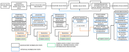
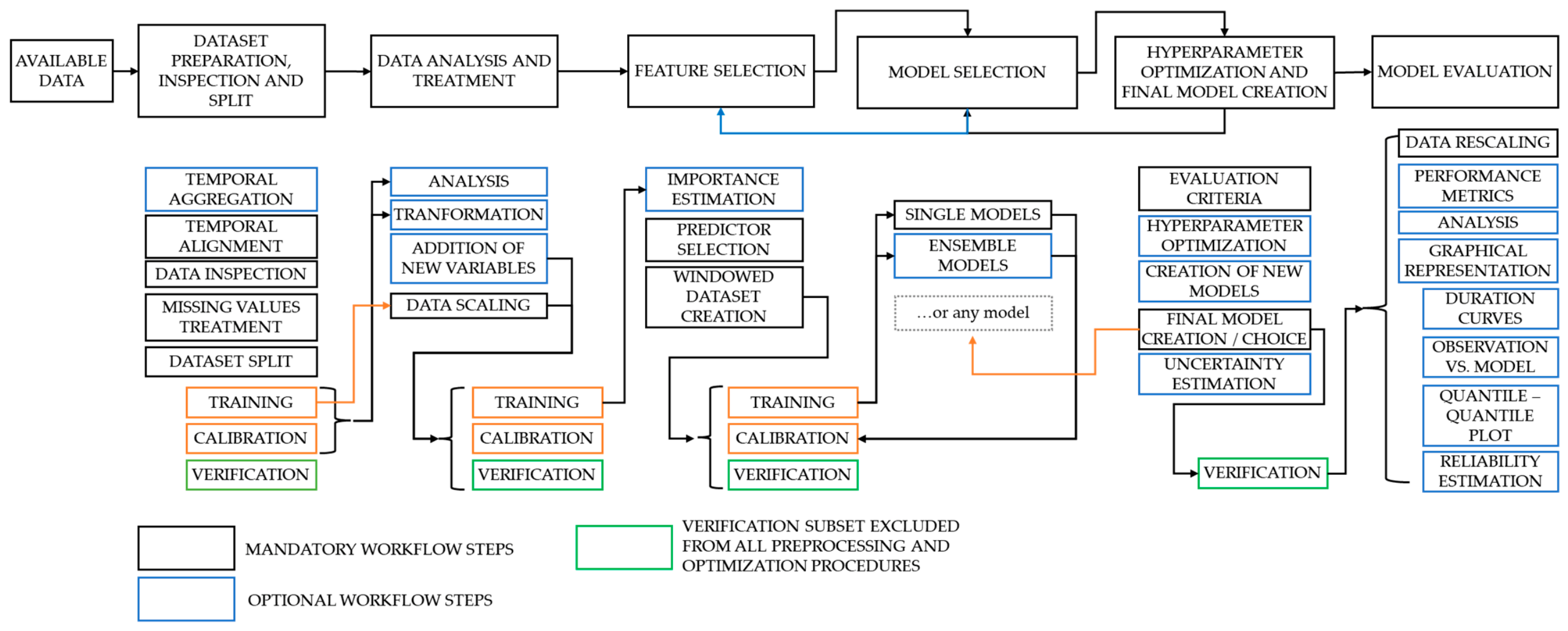
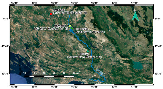
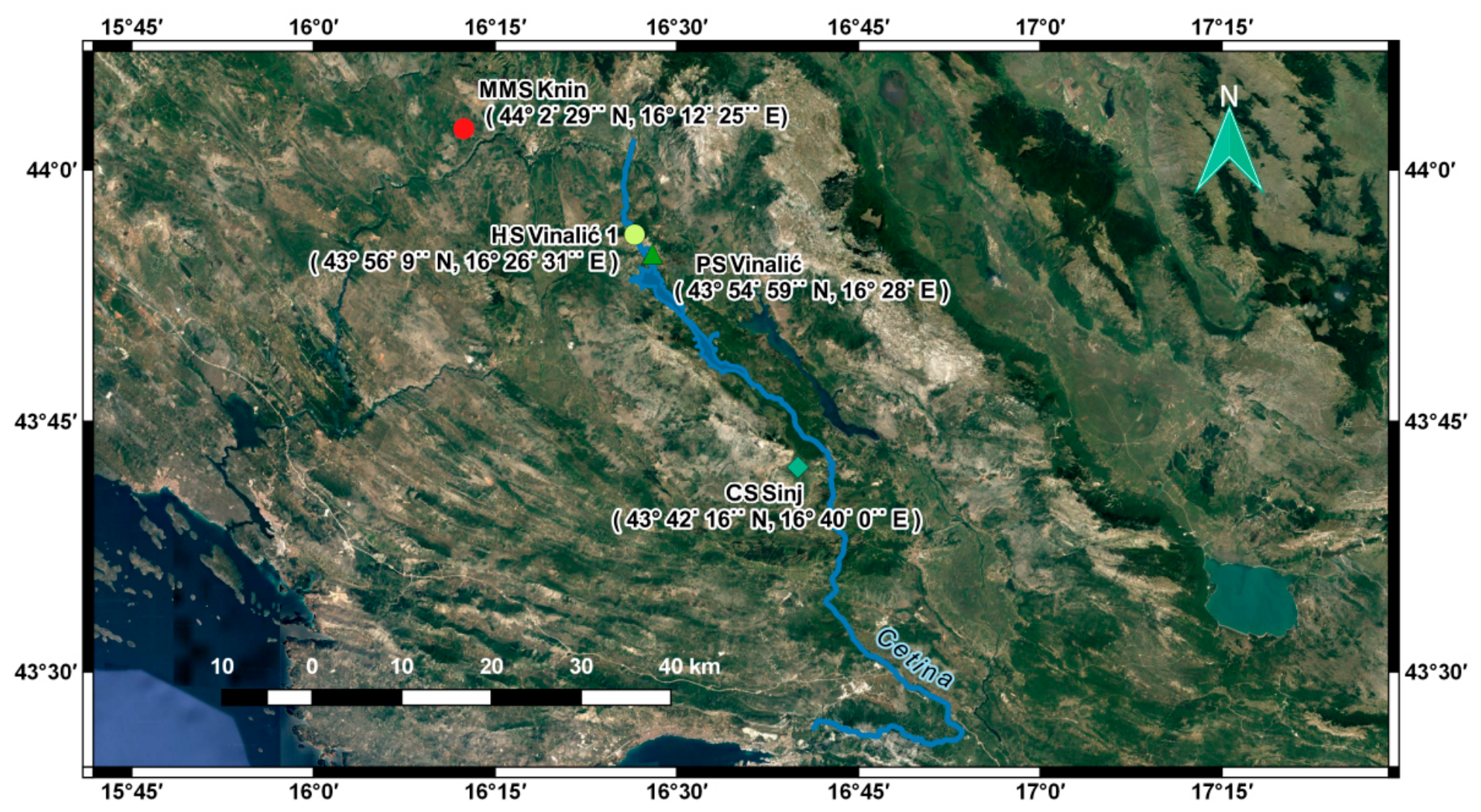
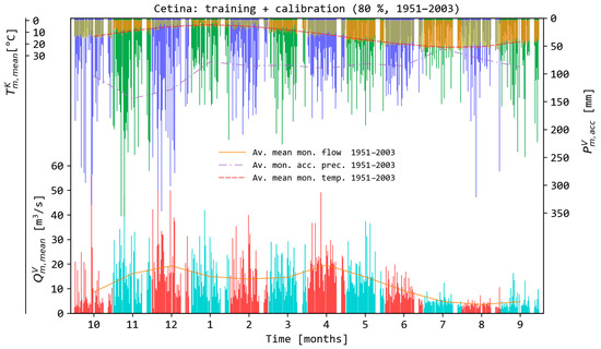
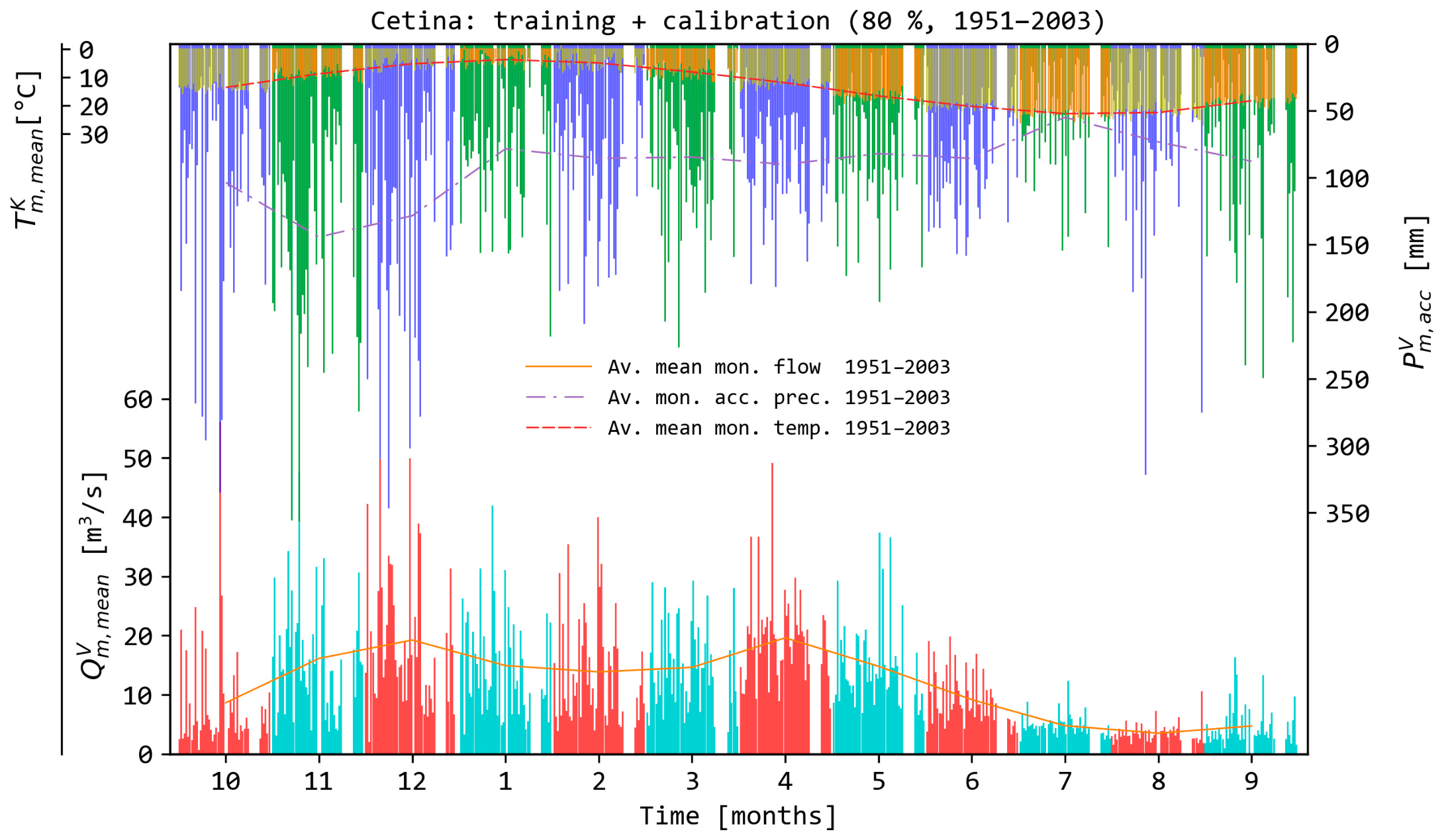
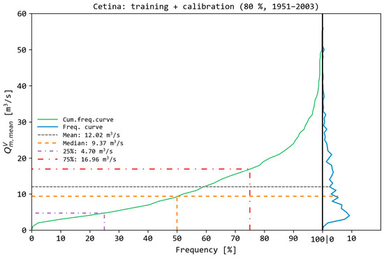
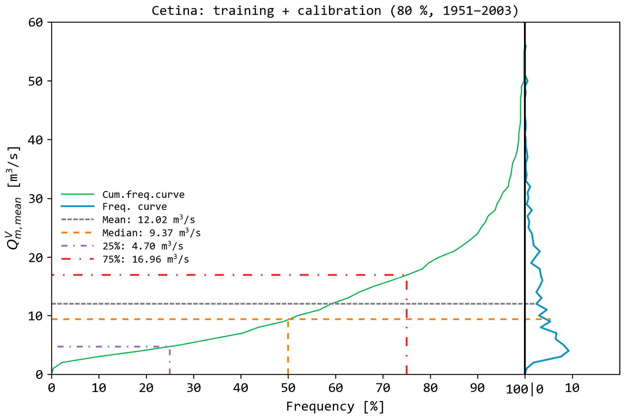
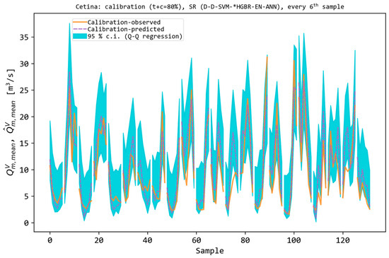
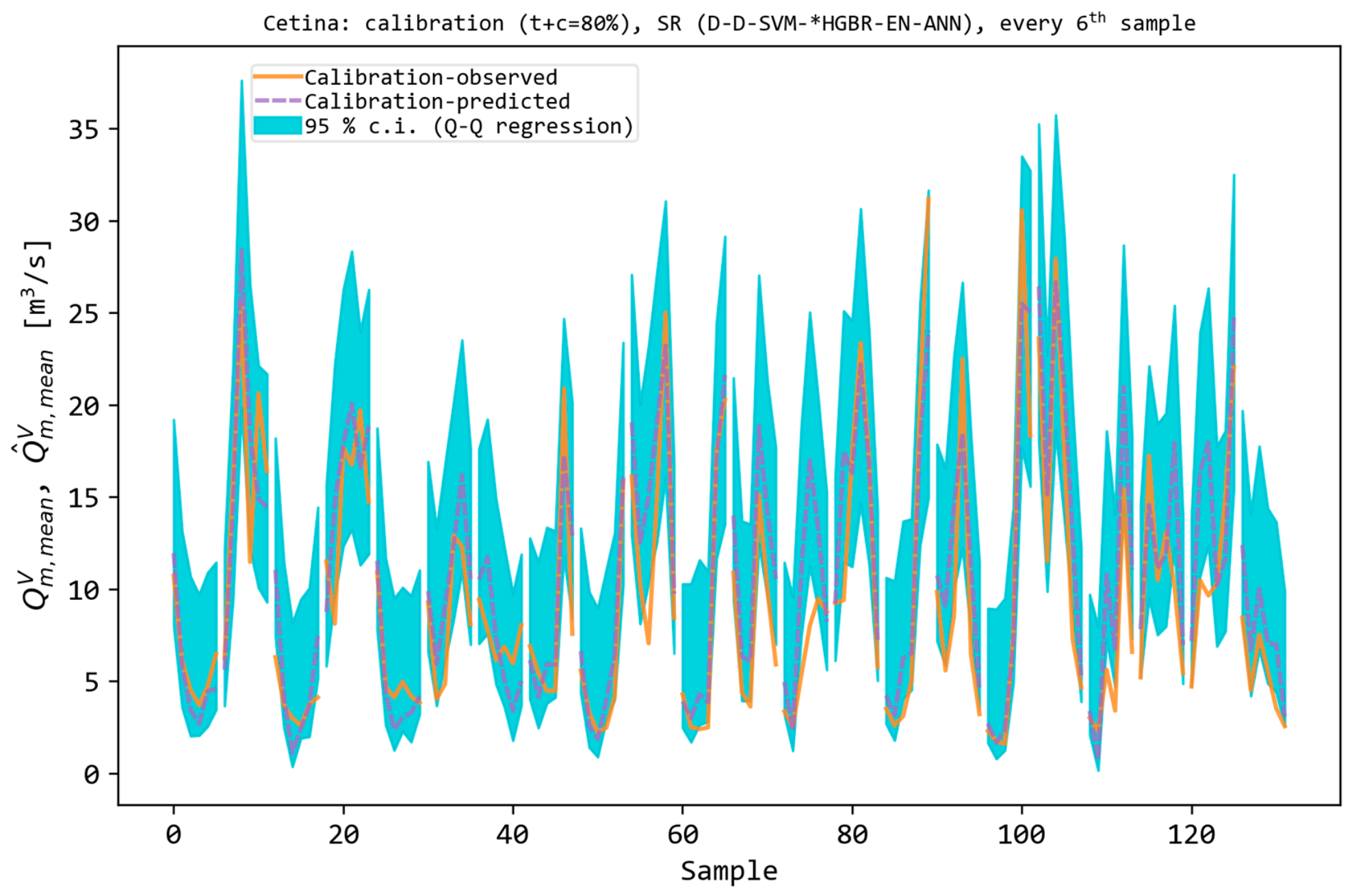
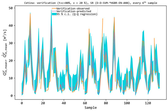
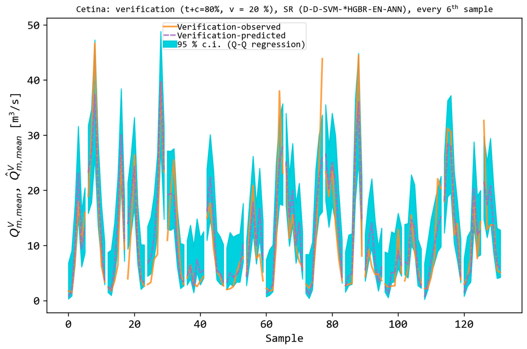
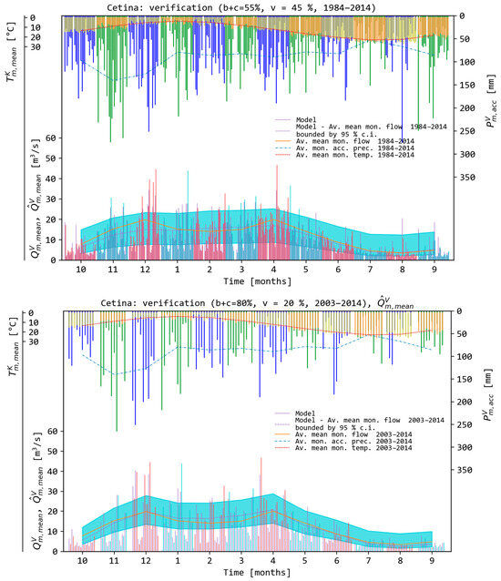
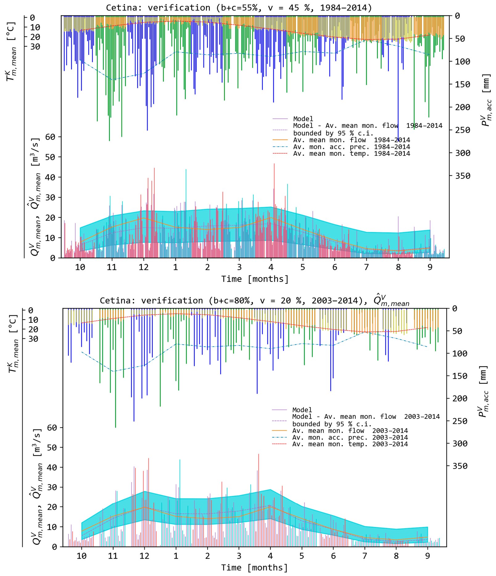
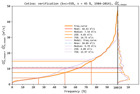
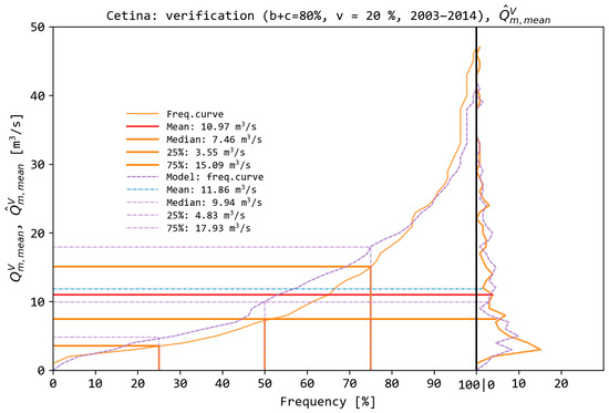
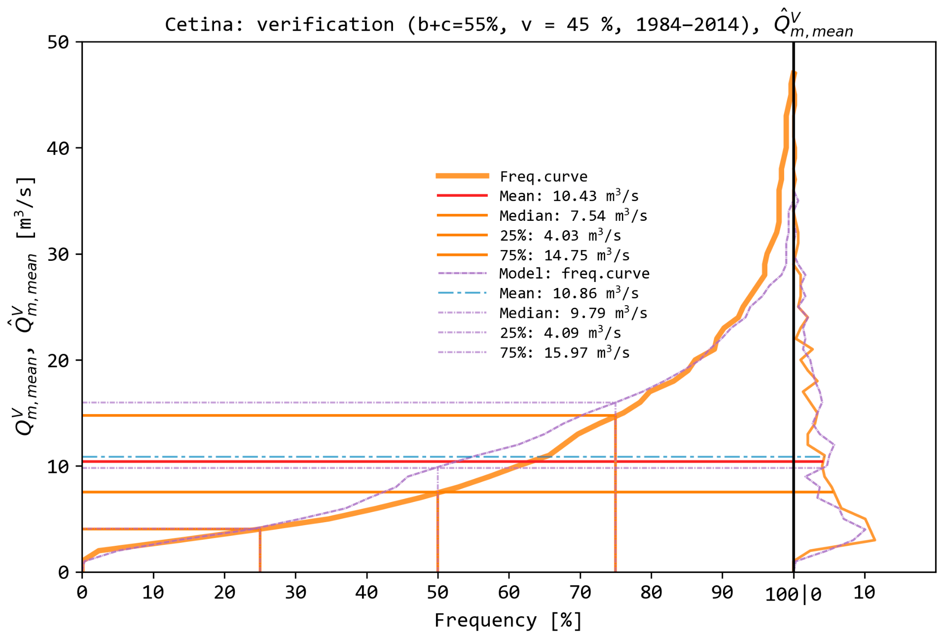
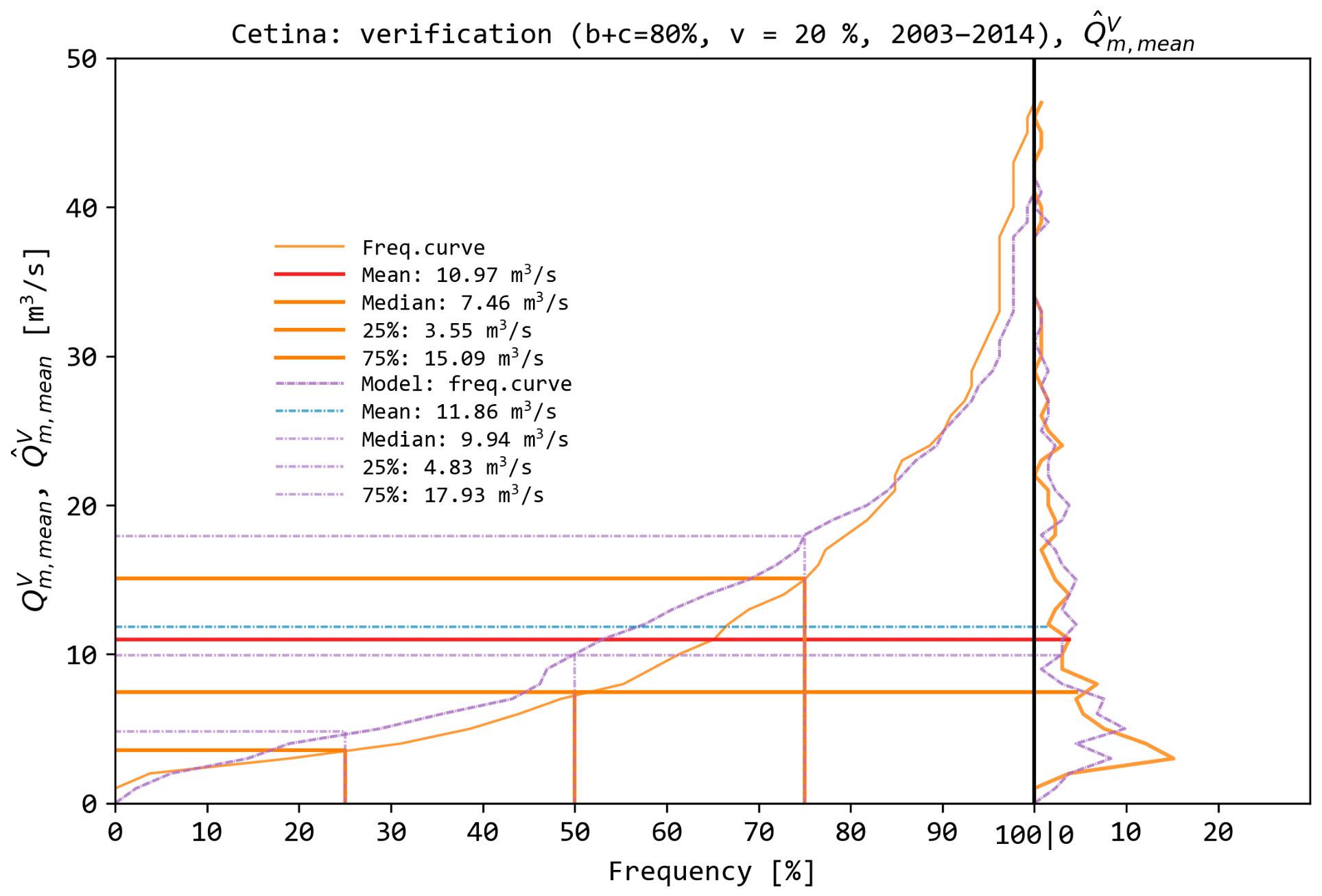
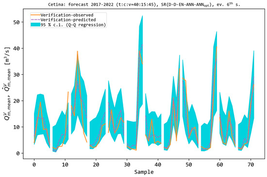
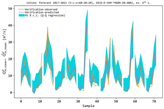
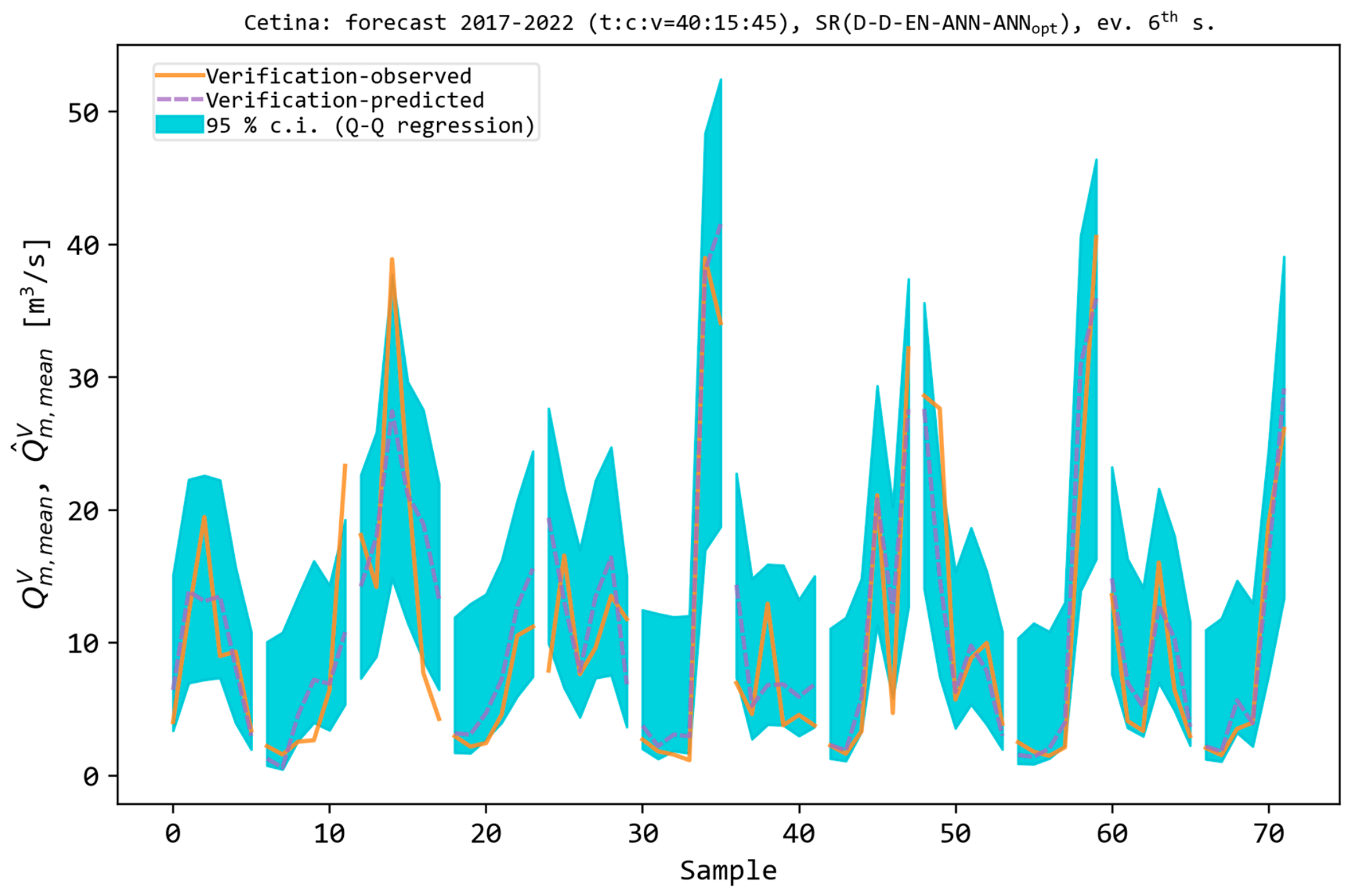
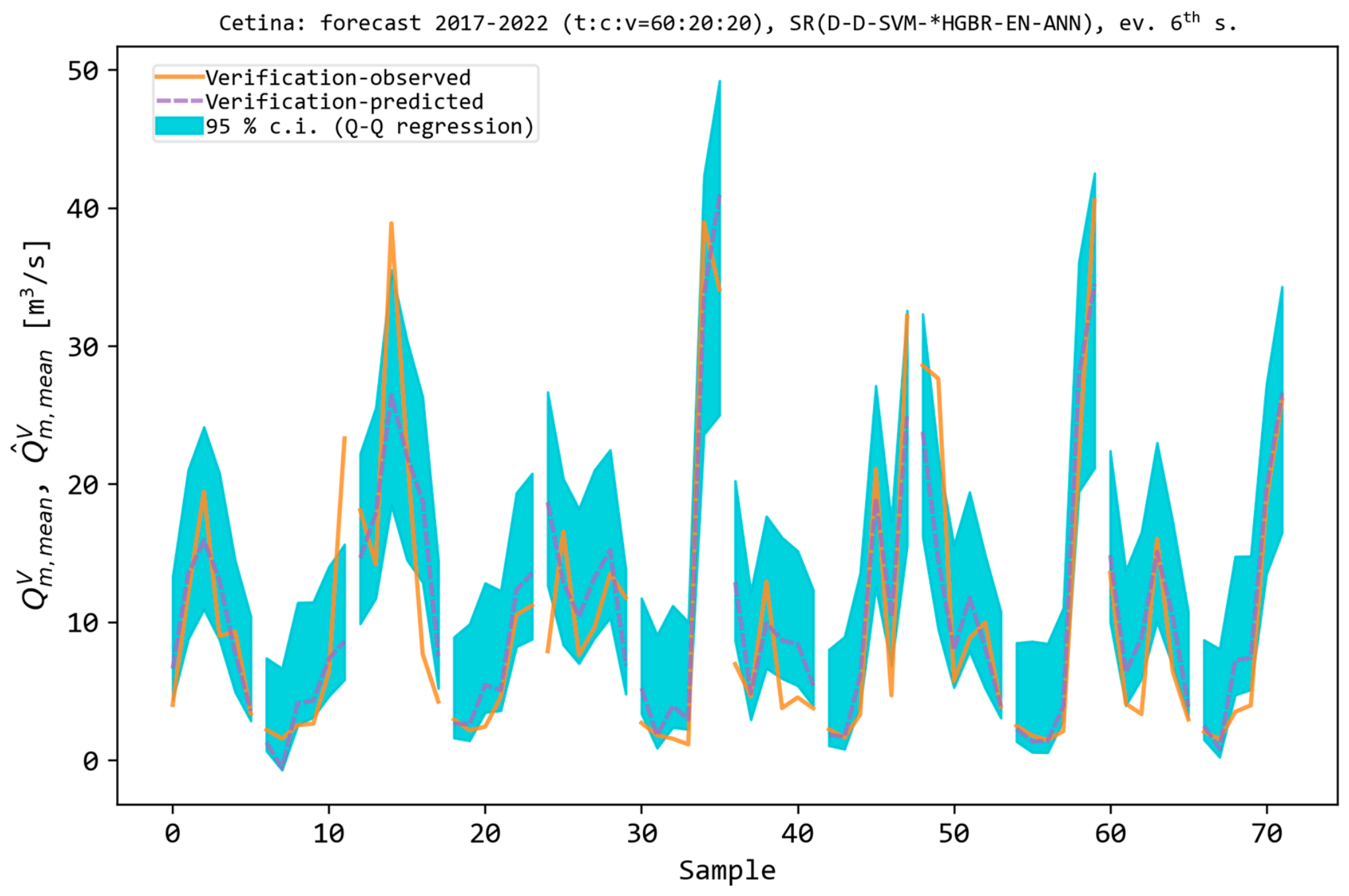
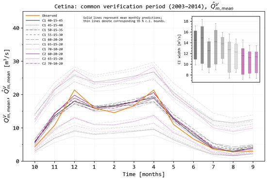
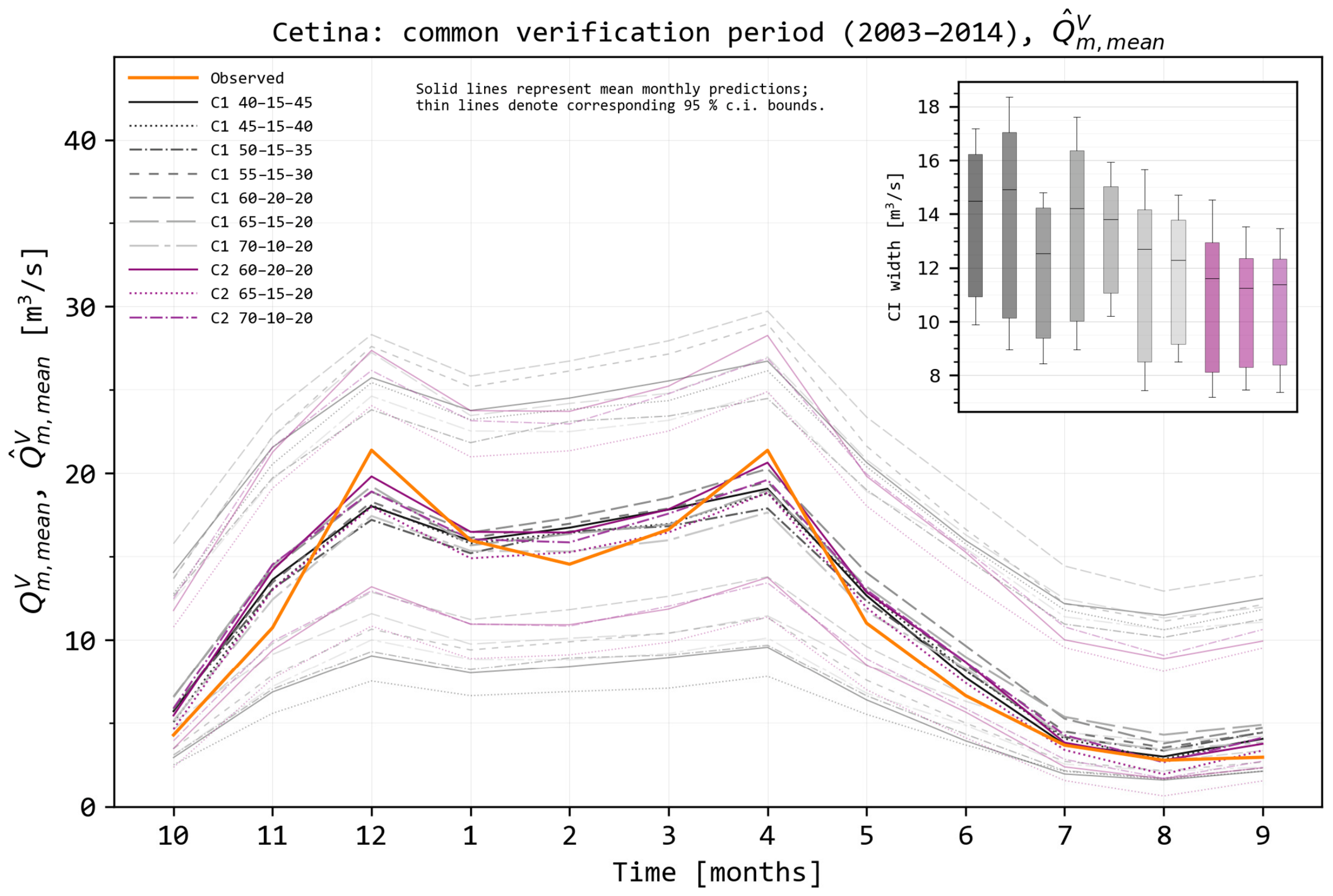
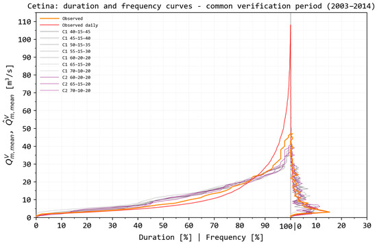
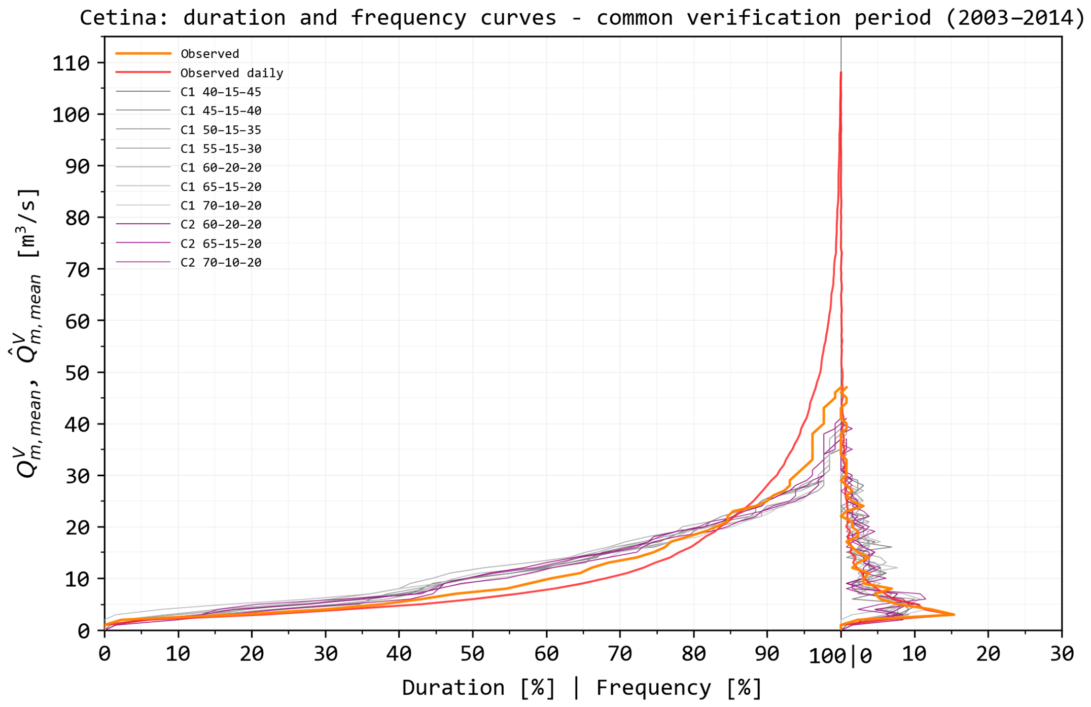
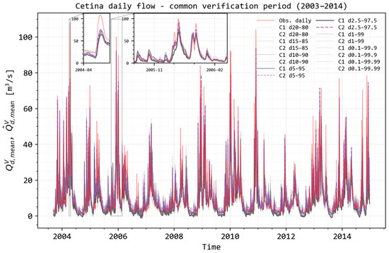
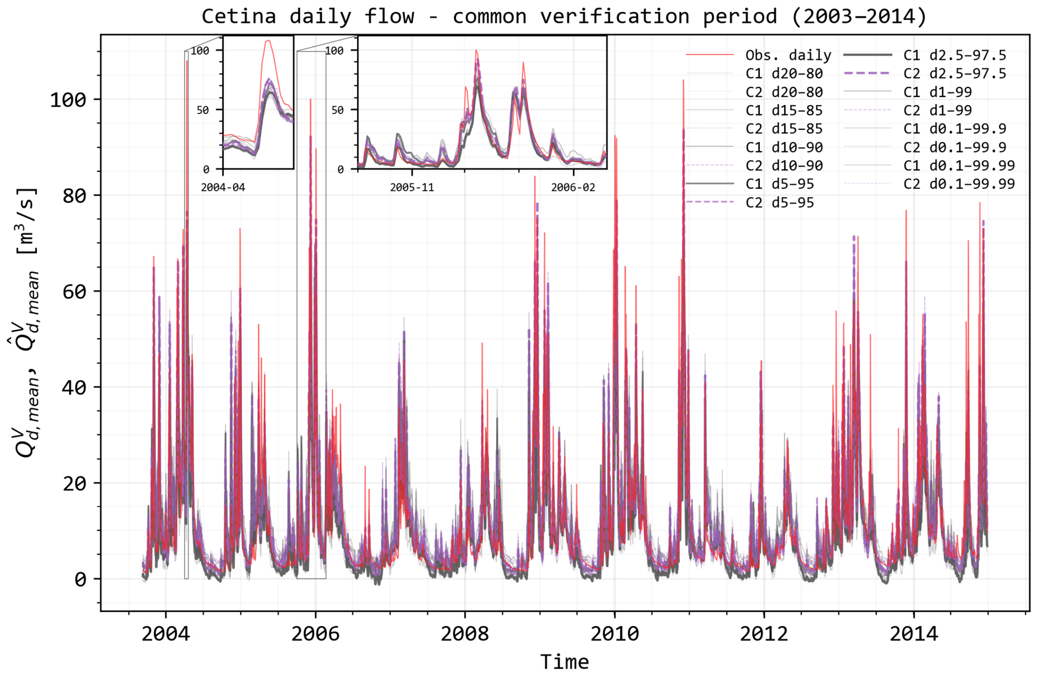
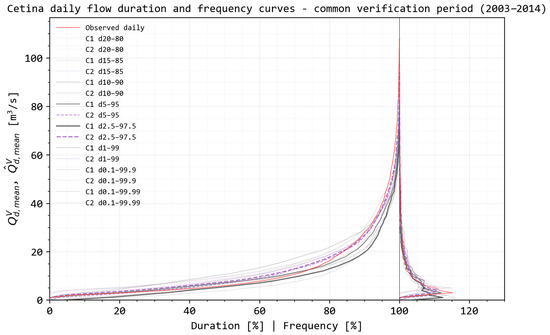
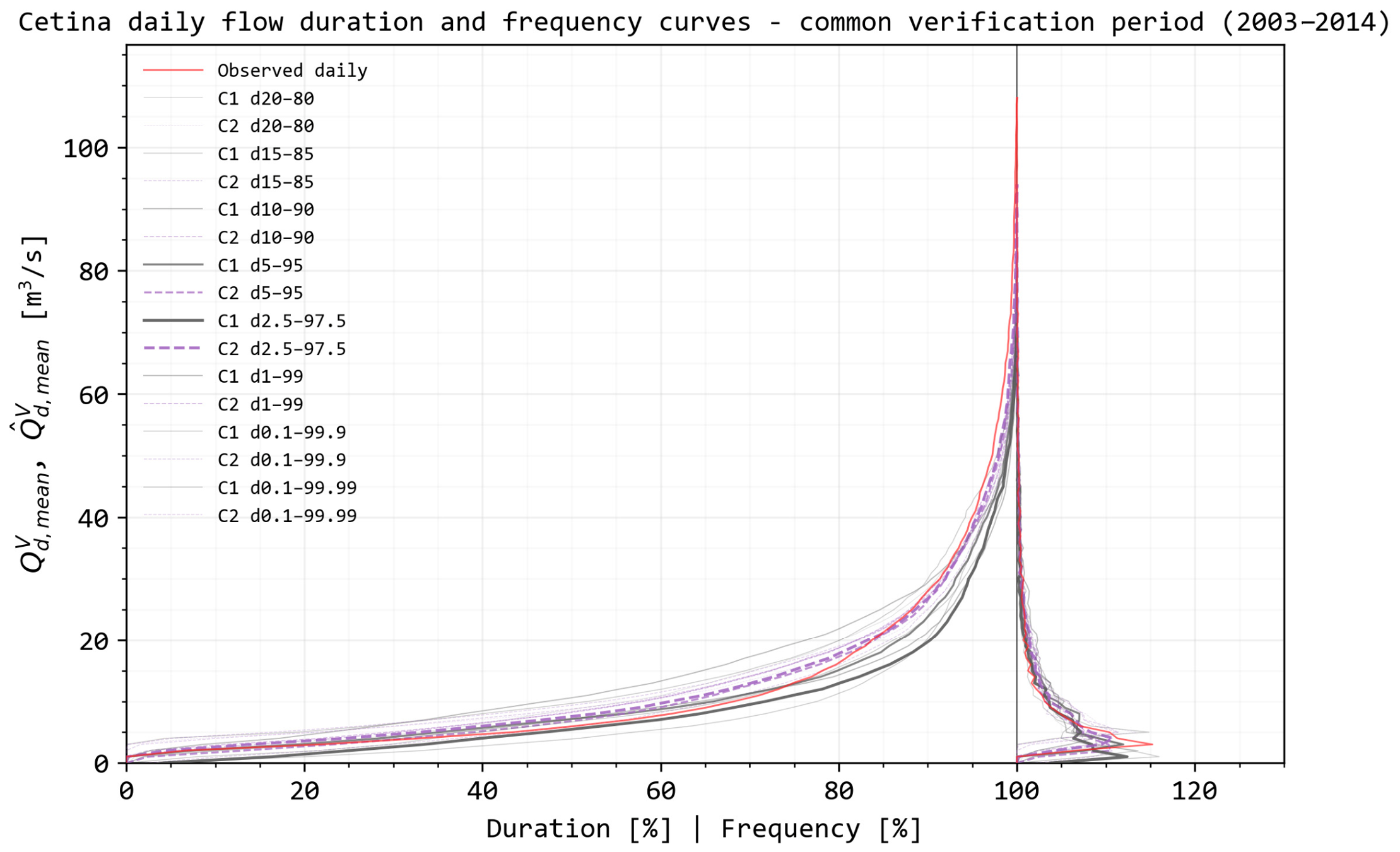

Disclaimer/Publisher’s Note: The statements, opinions and data contained in all publications are solely those of the individual author(s) and contributor(s) and not of MDPI and/or the editor(s). MDPI and/or the editor(s) disclaim responsibility for any injury to people or property resulting from any ideas, methods, instructions or products referred to in the content. |
© 2026 by the authors. Licensee MDPI, Basel, Switzerland. This article is an open access article distributed under the terms and conditions of the Creative Commons Attribution (CC BY) license.