Prediction and Uncertainty Quantification of Flow Rate Through Rectangular Top-Hinged Gate Using Hybrid Gradient Boosting Models

Abstract

Accurate estimation of flow discharge, Q, through hydraulic structures such as spillways and gates is of great importance in water resources engineering. Each hydraulic structure, due to its unique characteristics, requires a specific and comprehensive study. In this regard, the present study innovatively focuses on predicting Q through Rectangular Top-Hinged Gates (RTHGs) using advanced Gradient Boosting (GB) models. The GB models evaluated in this study include Categorical Boosting (CatBoost), Histogram-based Gradient Boosting (HistGBoost), Light Gradient Boosting Machine (LightGBoost), Natural Gradient Boosting (NGBoost), and Extreme Gradient Boosting (XGBoost). One of the essential factors in developing artificial intelligence models is the accurate and proper tuning of their hyperparameters. Therefore, four powerful metaheuristic algorithms—Covariance Matrix Adaptation Evolution Strategy (CMA-ES), Sparrow Search Algorithm (SSA), Particle Swarm Optimization (PSO), and Genetic Algorithm (GA)—were evaluated and compared for hyperparameter tuning, using LightGBoost as the baseline model. An assessment of error metrics, convergence speed, stability, and computational cost revealed that SSA achieved the best performance for the hyperparameter optimization of GB models. Consequently, hybrid models combining GB algorithms with SSA were developed to predict Q through RTHGs. Random split was used to divide the dataset into two sets, with 70% for training and 30% for testing. Prediction uncertainty was quantified via Confidence Intervals (CI) and the R-Factor index. CatBoost-SSA produced the most accurate prediction performance among the models (R² = 0.999 training, 0.984 testing), and NGBoost-SSA provided the lowest uncertainty (CI = 0.616, R-Factor = 3.596). The SHapley Additive exPlanations (SHAP) method identified h/B (upstream water depth to channel width ratio) and channel slope, S, as the most influential predictors. Overall, this study confirms the effectiveness of SSA-optimized boosting models for reliable and interpretable hydraulic modeling, offering a robust tool for the design and operation of gated flow control systems.

1. Introduction

1.1. General Description

The portable Rectangular Top-Hinged Gate (RTHG) is implemented as a simple and low-cost discharge measuring device, located along channels under free flow conditions. RTHG is hinged at the top horizontal axis of the gate, allowing it downward or upward movement [1]. RTHG operates through manual and hydraulic mechanisms. Its design allows water to pass when the gate swings upward or downward, while the vertical position corresponds to a closed state that effectively seals the waterway [2]. This type of sluice is applied as the measuring device and floodgate structure, typically constructed with steel, reinforced concrete, or timber, depending on the application. RTHG can be applied to regular water level management in irrigation canals and floodplain areas, flood control barriers, and urban water management systems [3]. Furthermore, regarding these RHTGs, the flow is consistently discharged through the underside of the gates, thereby reducing the likelihood of sediment deposition. Selecting appropriate RTHG dimensions is critical for enhancing the efficiency and overall performance of this measuring device in engineering applications. Figure 1 illustrates the schematic view of the RTHG and its affecting parameters.

Figure 1. Schematic view of the RTHG and definition of symbols [3].

Flow through RTHGs passes the gate opening and contracts to a minimum cross-section, generating a peak velocity before release. This contraction produces a distinct vena contracta downstream of the gate edge, which strongly governs discharge characteristics, pressure distribution, and the magnitude of energy losses. The degree of contraction depends on the gate opening and edge geometry: sharp-edged gates generate a more intense vena contracta, whereas rounded edges reduce contraction effects.

At higher velocities or larger openings, sharp edges can promote flow separation near the gate lip. This separation forms recirculation zones and increases turbulence intensity, which affects flow stability and energy dissipation, and may induce local vibrations, erosion, or structural stresses on the gate and canal bed. In many operating conditions, these separation-driven instabilities dominate the Energy Dissipation Mechanisms (EDMs) of RTHGs. Under sufficiently energetic flows, downstream hydraulic jumps may also form, further amplifying energy losses.

Because these hydraulic processes are inherently nonlinear—and depend simultaneously on geometry, opening ratio, and flow regime—developing explicit analytical formulations for predicting energy dissipation becomes challenging. The complex interaction between vena contracta formation, separation behavior, and turbulence necessitates data-driven modeling. Machine learning provides a practical approach to identify these nonlinear relationships and quantify EDMs across varying hydraulic and geometrical conditions, thereby improving gate design and operational efficiency.

1.2. Literature Review

Numerous studies have been conducted to assess the performance of RTHGs. Forster [4] evaluated the performance of these gates under both free-flow and submerged-flow conditions, and subsequently developed design equations and graphical methods to facilitate the design of RTHGs. This study and its design methodology were validated by Rajaratnam and Subramanya [5]. Furthermore, Rajaratnam and Subramanya [5] carried out extensive experiments on both free-flow and submerged-flow conditions to enhance the understanding of the performance characteristics of RTHGs.

Ramamurthy et al. [6] conducted an experimental investigation to evaluate RHTGs with cylindrical edges and observed that these configurations exhibited a high discharge coefficient (C_d) under submerged flow conditions. Burrows [7] and Burrows et al. [8] implemented the RTHG at the outfall to regulate the discharge (Q) rates into both the downstream tank and river outfalls. This regulation was achieved in accordance with a model developed in the principle of conservation of angular momentum. Swamee [9] presented a design criterion of RTHGs subject to free-flow conditions based on the study of Forster [4]. Raemy et al. [10] developed a comprehensive model for designing the RTHG as a control device to regulate upstream water elevations in small open channels.

Swamee et al. [11] developed comprehensive equations for calculating C_d under both free-flow and submerged-flow conditions, utilizing the ratio of upstream water depth to gate opening, h/P, as a key parameter. Litrico et al. [12] developed a mathematical model for the RTHG to automatically regulate upstream water levels in close proximity to a reference level, utilizing its own counterweight as the controlling mechanism. The validity of this mathematical model was confirmed through experimental data. Lozano et al. [13] compiled nearly 16,000 field data points and observed that C_d varies as a parabolic function of the gate opening (P). Belaud et al. [14] conducted a theoretical study to determine the contraction coefficient of RHTGs, enabling quick estimation of Q by applying principles of momentum and energy conservation between the upstream section and the contraction section.

Daneshfaraz et al. [2] examined the influence of the edge geometry on the variation in the contraction coefficient and the pressure distribution along the vertical surface of RTHGs. Vatankhah and Ghaderinia [15] employed a simple hinged semi-circular gate as a flowmeter for Q measurement in circular open channels under free-flow conditions, without the use of any counterweight. The design models for this type of gate were derived based on Buckingham’s theorem and experimental data, expressed as functions of the gate’s angular deviation and upstream water depth. Salmasi et al. [16] evaluated the water transfer capacity through inclined gates and observed an increase in C_d for vertical RTHGs. Moreover, the development of various predictive models for inclined RTHGs under both free-flow and submerged-flow conditions demonstrated that the Artificial Neural Network (ANN) approach provides the highest accuracy in comparison to alternative modeling techniques in predicting C_d. Gorgin and Vatankhah [3] conducted a series of extensive experiments to develop a comprehensive empirical model for predicting Q through the RTHG under free-flow conditions.

Boosting is an ensemble learning technique that integrates multiple weak learners, typically decision trees, to construct a robust predictive model. Boosting-based intelligent models are renowned for their high accuracy and efficiency in forecasting complex engineering phenomena. These models are capable of handling diverse data types and can mitigate overfitting through appropriate parameter tuning.

Numerous studies have explored the application of advanced boosting-based intelligent techniques to hydraulic performance and flood risk assessment. El Bilali and Taleb [17] employed a combination of real and Monte Carlo-simulated data to develop an XGBoost model for peak flow prediction under dam break scenarios, demonstrating robustness in data-limited conditions. Weekaew et al. [18] found AdaBoost outperformed other models, including XGBoost and Extra Trees Regressor, in predicting flow over stepped spillways. Azma et al. [19] evaluated Gradient Boosting, XGBoost, and CatBoost for estimating discharge-related parameters of gabion weirs, with CatBoost achieving the best performance in predicting through-flow discharge ratios. Further, Asgharzadeh-Bonab et al. [20] developed multiple models—including TabNet optimized with Moth Flame Optimization, ELM enhanced with Jaya and Firefly algorithms, Decision Trees, and LightGBM—to predict discharge coefficients of semicircular labyrinth weirs. The results indicated the TabNet-MFO model remained the top performer as a metaheuristic framework, followed by ELM-JFO, LightGBM, and DT models. Belaabed et al. [21] compared optimized versus non-optimized models, revealing that bio-inspired optimization significantly enhanced NGBoost and XGBoost performance. Bansal et al. [22] demonstrated that XGBoost outperformed Gene Expression Programming in predicting energy losses in type-C PKWs. Similarly, Abdi Chooplou et al. [23] found that MLP and XGBoost provided superior predictions for scour hole parameters downstream of PKWs. Afaridegan et al. [24] highlighted CatBoost’s high accuracy in estimating the energy dissipation rate of modified semi-cylindrical weirs, with hybrid models further improving performance. Dhar et al. [25] confirmed CatBoost as the top performer in predicting discharge coefficients of rectangular sharp-crested weirs. Shirvan et al. [26] reported CatBoost’s superior accuracy over traditional nonlinear regression and gene expression programming in estimating discharge coefficients of partially blocked weirs. Bijanvand et al. [27] identified CatBoost and TabNet as the most accurate models for harmonic plan circular weirs. Afaridegan et al. [28] demonstrated that hybrid models combining boosting algorithms such as LightBoost, NGBoost, and TabNet with optimization techniques significantly improved the accuracy of discharge coefficient predictions for hydrofoil-crested spillways.

1.3. Research Objectives and Novelties

The primary objective of this study is the accurate estimation of Q passing through a RTHG using hybrid models based on gradient boosting algorithms. The models employed include Categorical Boosting (CatBoost), Natural Gradient Boosting (NGBoost), Histogram-based Gradient Boosting (HistGBoost), Extreme Gradient Boosting (XGBoost), and Light Gradient Boosting (LightGBoost). Four powerful metaheuristic algorithms—CMA-ES (Covariance Matrix Adaptation Evolution Strategy), SSA (Sparrow Search Algorithm), PSO (Particle Swarm Optimization), and GA (Genetic Algorithm)—were evaluated and compared for hyperparameter tuning. Outlier removal was performed using the Local Outlier Factor (LOF) algorithm, and data normalization was carried out via Z-score normalization. To identify the effective dimensionless independent parameters influencing the modeling of flow rate through the RTHG, Dimensional Analysis and Analysis of Variance (ANOVA) were conducted. The dataset was split into 70% for training and 30% for testing. Model performance was evaluated using comprehensive and standard metrics including the Coefficient of Determination (R²), Root Mean Square Error (RMSE), Mean Absolute Error (MAE), Mean Absolute Percentage Error (MAPE), and Percent Bias (PBIAS). Additionally, model comparison and ranking were performed using the Taylor Diagram. Sensitivity analysis was conducted using the SHapley Additive exPlanations (SHAP) method, while uncertainty quantification of the hybrid models was assessed through Confidence Interval (CI) and R-Factor indices. To date, no comprehensive study has focused on predicting Q through RTHGs. This research takes an innovative approach by examining the impact of metaheuristic algorithms on hyperparameter optimization, model performance, and prediction accuracy of gradient boosting models, while also evaluating prediction uncertainty, providing a systematic and complete framework for the design and operation of gated flow control systems.

2. Materials and Methods

2.1. Data Collection and Experimental Setup

The dataset used in this study originates entirely from the laboratory experiments of Gorgin and Vatankhah [3], who examined the hydraulic performance of a Rectangular Top-Hinged Gate (RTHG) installed in a rectangular open channel under free-flow conditions. No additional physical experiments were conducted by the present authors; all analyses in this paper are based on the experimental data published in [3].

The experiments in [3] were carried out in the hydraulic laboratory of the Irrigation and Reclamation Engineering Department at the University of Tehran, Iran. The facility consists of a 12 m long, 0.25 m wide and 0.5 m deep rectangular channel that can be operated with two longitudinal slopes, S = 0 and S = 0.005; see Figure 2. The flow is supplied from a large upper reservoir with nearly constant water level, through a pump and an inlet stilling section, which reduces free-surface fluctuations before the flow reaches upstream of the gate.

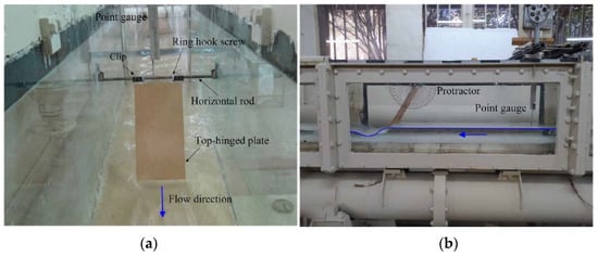
Figure 2. RTHG during an experiment and its elements. (a) Front view and (b) side view [3].

At the downstream end of the channel, the discharge passes over a sharp-crested triangular weir and then enters an underground reservoir. For higher discharges, a sharp-crested rectangular weir installed in the recirculation loop is used as an additional measuring structure. Both weirs were calibrated by means of an electromagnetic flow meter with a nominal accuracy of about 0.5% of full scale, and the resulting rating curves were adopted as the primary discharge measurement devices in all tests. During each run, the discharge was kept constant by adjusting a flow-control valve, while any excess water from the upper reservoir was bypassed to the underground tank.

The upstream water depth h was measured along the centerline of the channel using a point gauge with a nominal accuracy of 0.1 mm. The gauge was located approximately 0.8 m upstream of the RTHG to avoid the influence of local disturbances near the gate. In the original experiments of [3], no pressure transducers were used; therefore, all water-level data employed in the present study are based on these point-gauge readings. The deflection angle θ of the RTHG was read from a mechanical protractor mounted at the top hinge of the gate.

The RTHGs were fabricated from Plexiglas sheets with thicknesses t equal to 5 and 10 mm. The gate lengths were L = 0.20 and 0.30 m, and the gate widths b ranged from 0.05 to 0.20 m in increments of 0.05 m. The gates were installed at the mid-width of the channel, with their lower edge positioned approximately 5 mm above the channel bed. All gate edges were beveled to form sharp crests and to promote a well-defined flow contraction. The gates were hinged at the top by low-friction ring hook screws and a horizontal steel rod with a diameter of 5 mm, which acted as the pivot. Depending on their dimensions, the gate masses varied between 0.061 and 0.692 kg.

In total, 687 steady-flow tests were performed in [3], consisting of 393 runs for S = 0 and 294 runs for S = 0.005. The discharges covered the range Q = 1–74 L/s, with gate deflection angles between approximately 3.5° and 81°. The depth ratio h/B varied between 0.065 and 0.95, while the width ratio b/B ranged from 0.2 to 0.8. This experimental database forms the complete set of observations used in the present work to train and evaluate the proposed GBM models.

A detailed error analysis of the empirical discharge equations derived from this dataset is provided in [3]. Their unified relations exhibit relative errors of about 2.3–3.3%, and approximately 80–90% of the measured discharges lie within ±5% of the observed values. In the present study, this range is adopted as a representative estimate of the experimental uncertainty in the discharge data used for model development and validation. The instrument-level uncertainties in water depth (on the order of ±0.1 mm) and in angle readings are significantly smaller than the observed scatter in Q and are therefore not propagated explicitly through the machine-learning models. Table 1 lists the experimental measurements obtained for S = 0 and S = 0.005, respectively, for free-flow conditions.

Table 1. The statistical range of parameters in this study.

Parameter	S = 0				S = 0.005
	Min	Median	Max	SD	Min	Median	Max	SD
Q (m3/s)	0.001	0.017	0.074	0.019	0.001	0.020	0.069	0.019
h (m)	0.020	0.010	0.238	0.057	0.016	0.093	0.226	0.053
θ (degree)	4.0	42.5	81.0	20.0	3.5	45.5	80.0	20.4
b (m)	0.05	0.10	0.20	0.06	0.05	0.15	0.20	0.05
L (m) 1	0.20	0.30	0.30	0.05	0.20	0.20	0.30	0.05
t (m) 2	0.005	0.005	0.010	0.002	0.005	0.005	0.010	0.003

Note(s): ¹ L is the top-hinged gate length; ² t is the top-hinged gate thickness.

2.2. Dimensional Analysis

Dimensional analysis is an essential tool in engineering and applied sciences that allow the simplification of complex physical relationships, making them more generalizable. By converting various parameters into dimensionless groups, it is possible to assess the influence of different factors without dependence on measurement units and reducing the number of input variables in a model [29]. This approach not only facilitates analysis and design but also enhances the accuracy and stability of predictive models. Especially in hydraulic problems, such as estimating Q through different gates, dimensional analysis plays a key role in identifying influential parameters and optimizing models. Accordingly, the effective parameters influencing Q through the RTHGs are presented in Equation (1).

$$Q=f\left(h,B,b,L,t,S,\theta ,g,\mu ,\rho ,\sigma \right)$$

(1)

where h is the upstream water depth; B is the width of the rectangular open channel; b is the width of the RTHG; L is the length of the RTHG; t is the thickness of the gate; S is the longitudinal slope of the channel; θ is the deflection angle of the RTHG; g is the acceleration due to gravity; μ is the dynamic viscosity of water; ρ is the density of water; and σ is the surface tension of water. The effective dimensionless parameters were extracted using Buckingham π theorem and are presented in Equation (2):

$${\displaystyle \frac{Q}{\sqrt{g{h}^5}}}=f\left({\displaystyle \frac{h}{B}},{\displaystyle \frac{L}{b}},{\displaystyle \frac{t}{B}},S,\theta ,\mathrm{R},\mathrm{W}\right)$$

(2)

in which R is the Reynolds number and W the Weber number. Since the minimum gate opening in this study is greater than the specified minimum value (2 cm) and the flow is fully turbulent, the effects of R and W can be neglected. Based on these considerations, Equation (2) is rewritten as Equation (3):

$${\displaystyle \frac{Q}{\sqrt{g{h}^5}}}=f\left({\displaystyle \frac{h}{B}},{\displaystyle \frac{L}{b}},{\displaystyle \frac{t}{B}},S,\theta \right) .$$

(3)

Analysis of Variance (ANOVA) was used as a statistical method to examine the effect of the independent variables (h/B, L/b, t/B, S, and θ) on the dependent variable (Q/√gh⁵). The purpose of this method was to identify parameters that cause significant variations in the flow rate and thus play an important role in modeling. The results of this analysis are presented in Table 2, which also shows the p-value for each parameter; parameters with very small p-values (e.g., less than 0.05) indicate a statistically significant effect on the model.

Table 2. Statistical summary and ANOVA results for dimensionless parameters influencing normalized Q through the RTGH.

Feature	Min	Max	Median	p-Value
Q/√gh5	0.018	11.184	1.965	-
h/B	0.065	0.950	0.389	8.198 × 10−10
L/b	1.0	6.0	2.0	1.604 × 10−19
t/B	0.02	0.04	0.02	2.436 × 10−12
θ	3.5	81.0	43.5	2.453 × 10−15
S	0.000	0.005	0.000	1.380 × 10−39

Based on the results of Table 2, all the dimensionless variables h/B, L/b, t/B, S, and θ have very small p-values, indicating that each parameter has a statistically significant effect on the normalized flow rate (Q/√gh⁵). This confirms that these parameters are important factors influencing Q through the RTHG and must be considered in the modeling process. In Figure 3, the distribution of dimensionless parameters derived from Equation (3) is presented as violin plots. Each violin plot represents the probability density distribution and variability of the data corresponding to each dimensionless parameter.

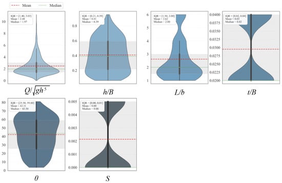
Figure 3. Distribution of dimensionless parameters influencing the modeling of Q through the RTHG.

2.3. Outlier Detection Using Local Outlier Factor (LOF) and Preprocessing

Before training the hybrid gradient boosting models, the experimental dataset was carefully examined and preprocessed. The original data, compiled from the laboratory experiments of Gorgin and Vatankhah [3], did not contain missing values. Therefore, no data imputation, interpolation, or temporal smoothing was required, and data cleansing was focused on the detection of anomalous runs and on the normalization of the modeling variables.

Outlier detection was conducted using the Local Outlier Factor (LOF) algorithm. LOF evaluates the local density of each observation relative to its neighbors and assigns a score that quantifies how isolated a point is with respect to the surrounding data. In this study, LOF scores were computed in the multidimensional feature space, and samples with significantly lower local density, that is, with markedly elevated LOF scores, were considered anomalous and removed from the dataset. This procedure allowed us to discard a small number of physically inconsistent runs while preserving the large majority of the experimental observations. The resulting LOF-filtered dataset was used consistently for the development and assessment of all gradient boosting models (Cheng et al. [30]). Figure 4 illustrates the original data along with the identified normal points and outliers.

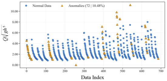
Figure 4. Distribution of normal and outlier data points identified using LOF.

After outlier removal, all variables were expressed in dimensionless form, namely the upstream depth ratio h/B, gate-length ratio L/b, thickness ratio t/B, bed slope S, gate angle θ, and the dimensionless discharge Q/√(gh⁵). To place these predictors and the target on a comparable numerical scale and to improve the numerical conditioning of the learning algorithms, Z-score normalization was applied. For a generic variable x, the standardized value x* was computed as:

$$x^{*}={\displaystyle \frac{x-\zeta }{{\sigma }_x}}$$

(4)

where ζ and σ_x denote the mean and standard deviation of x, respectively. The normalization parameters were estimated from the training subset, and the same transformation was then applied to the test subset to avoid information leakage.

Finally, the cleaned and normalized dataset was randomly partitioned into training and testing subsets. A random 70/30 split was adopted, with 70% of the samples allocated to model training and hyperparameter tuning and the remaining 30% reserved exclusively for model evaluation. Given that the target variable (flow rate) is continuous and that the experimental data are relatively well distributed over the investigated hydraulic and geometric ranges, no explicit stratification of the split was applied. The random partition was generated with a fixed random seed to ensure reproducibility of the results across all hybrid gradient boosting models.

2.4. Gradient Boosting Models

For predicting Q through the RTHGs, five GB models, including XGBoost, LightGBoost, CatBoost, NGBoost, and HistGBoost, were used. In this process, the data is randomly split into two parts: 70% for model training and 30% for model evaluation. This division allows the model to first learn from the training data and then evaluate its performance on the test set. Gradient Boosting models utilize iterative decision trees to minimize prediction errors and are capable of modeling complex relationships within the data. These models are particularly suited for data with complex, nonlinear features, such as Q through RTHGs. A flowchart of the study is shown in Figure 5.

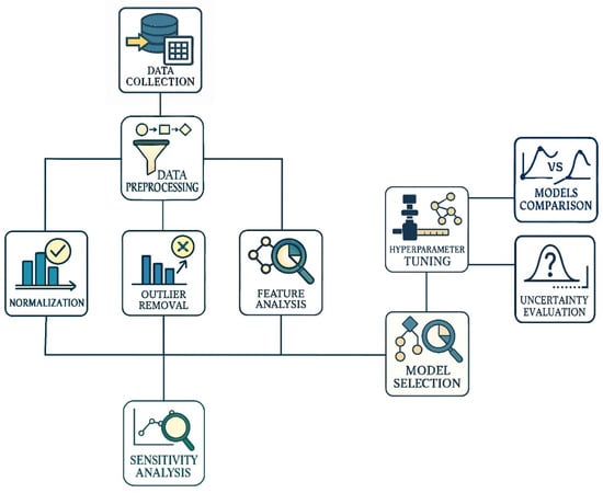
Figure 5. Flowchart of the research methodology adopted in this study.

2.4.1. Histogram-Based Gradient Boosting (HistGBoost)

HistGBoost is a variant of the GB algorithm that has been developed to be used on large datasets using histogram binning. This transforms continuous features into bins, reducing memory usage as well as training time. HistGBoost compromises between performance and speed by approximating gradient statistics through histograms, thus it is suitable for large-scale machine learning applications (Guryanov [31]).

The key features of HistGBoost can be listed as follows. (i) Efficiency: HistGBoost reduces memory consumption and speeds up splitting in building a tree, especially when working with big datasets; (ii) Scalability: It is highly scalable as it can consume vast amounts of data and process them efficiently; (iii) Early Stopping: For the prevention of overfitting, HistGBoost offers early stopping, where learning can be terminated once progress on the validation set stops.

Table 3 summarizes these hyperparameters along with their abbreviations and short descriptions for easy reference.

Table 3. Key hyperparameters of the HistGBoost model.

Hyperparameter	Abbreviation	Explanation
Learning Rate	LR	Controls the step size at each boosting iteration to prevent overfitting. Smaller values usually improve accuracy but require more iterations.
Maximum Iterations	MI	Maximum number of boosting iterations (trees) to be built. Determines how long the model trains.
Maximum Leaf Nodes	MLN	Maximum number of leaves per tree. Controls the complexity of each tree and helps prevent overfitting.
Early Stopping	ES	Enables early stopping by monitoring validation metrics to halt training when no improvement is observed for a set number of iterations.

2.4.2. Categorical Boosting (CatBoost)

CatBoost is a cutting-edge GB algorithm based on decision trees, specially designed to be used in tabular data with categorical features. CatBoost provides revolutionary ways to process categorical variables efficiently without pre-requiring the application of laborious preprocessing methods like one-hot encoding or label encoding, which can sometimes result in information loss or issues of dimensionality (Dorogush et al. [32]).

The principal features of CatBoost can be summarized as follows. (i) Categorical Feature Processing: CatBoost’s first innovation is that it can natively handle categorical features without time-consuming preprocessing like one-hot or label encoding. It improves performance and reduces data preprocessing steps; (ii) Ordered Boosting: Ordered boosting is a breakthrough of CatBoost and is employed to prevent prediction shift that typically happens because of traditional gradient boosting methods. This prevents overfitting and improves the generalization of the model to new data overall; (iii) Symmetric Trees: Symmetric trees are employed by the model, wherein each leaf of a tree is split in a similar fashion, which improves the precision of the predictions and prevents overfitting; (iv) Effective Implementation: CatBoost supports multi-threading and GPU acceleration, which enables rapid training on large data. This makes CatBoost scalable and usable for a wide range of machine learning tasks like classification, regression, ranking, and time-series forecasting; (v) Regularization: The algorithm possesses effective regularization techniques that prevent overfitting and deliver satisfactory results on new samples [24].

Table 4 presents the primary hyperparameters of the CatBoost model along with their common abbreviations and short descriptions.

Table 4. Key hyperparameters of the CatBoost model.

Hyperparameter	Abbreviation	Explanation
Learning Rate	LR	Step size shrinkage used to prevent overfitting by controlling how much the model is updated per iteration. Lower values typically yield better accuracy but require more iterations.
Depth	DP	Maximum depth of the individual trees. Deeper trees can model more complex relationships but risk overfitting. Typical values range between 4 and 10.
L2 Regularization	L2R	L2 regularization coefficient applied to leaf values. Helps reduce model complexity and overfitting by penalizing large leaf weights.
Verbose	VB	Controls the verbosity of the training process output. When set to true or a positive integer, training progress and metrics are printed.

2.4.3. Light Gradient Boosting Machine (LightBoost)

LightGBoost is a highly effective, distributed, and high-performance GB framework with decision tree algorithms. It is optimized to be fast and scalable and hence it is a very good choice for large machine learning tasks. LightGBM is optimized to learn efficiently, with high precision and low memory, and it is widely utilized for jobs like classification, regression, and ranking (Oram et al. [33]).

The principal features of LightGBM can be summarized as follows. (i) Histogram-Based Algorithm: LightGBM uses histogram-based algorithms to reduce memory usage and accelerate training through the discretization of continuous features into histograms; (ii) Leaf-Wise Tree Growth: LightGBM follows leaf-wise growth for trees instead of level-wise growth [20]. It grows the tree by choosing the leaf with the highest potential for improvement, leading to improved accuracy and faster convergence but occasionally leading to overfitting with too many leaves; (iii) Handling Categorical Features: LightGBM offers explicit handling of categorical features without needing to transform them (e.g., one-hot encoding), saving memory and computation costs; (iv) Scalability and Efficiency: LightGBM handles large datasets efficiently and works well even on enormous amounts of data. It can utilize multi-threading and distributed learning, so it is appropriate for high-performance settings; (v) Early Stopping: The algorithm supports early stopping, a feature that prevents training the model when its performance on a validation set no longer increases after a specified number of iterations; (vi) Feature Importance: Automatic feature importance computation is supported by LightGBM, such that users can identify what features are most accountable for the predictions of the model [28].

To make LightGBM as efficient as possible, some important hyperparameters must be adjusted. The hyperparameters enable the adjustment of the accuracy vs. training speed trade-off. Table 5 summarizes these hyperparameters with acronyms and brief descriptions.

Table 5. Key hyperparameters of the LightGBoost model.

Hyperparameter	Abbreviation	Explanation
Learning Rate	LR	Controls the step size at each iteration. Smaller values improve accuracy but require more iterations.
Number of Leaves	NL	Maximum number of leaves in one tree. More leaves increase model complexity and risk overfitting.
Minimum Child Samples	MCS	Minimum number of data needed in a child (leaf). Used to control overfitting.
Verbose	VB	Controls the verbosity of the training output.

2.4.4. Natural Gradient Boosting (NGBoost)

NGBoost is a high-end probabilistic framework for boosting that generalizes traditional gradient boosting to produce full predictive distributions instead of point predictions. NGBoost is very useful in risk-sensitive applications, where not just the prediction but also the prediction uncertainty is important (Duan et al. [34]).

The principal features of NGBoost can be summarized as follows. (i) Probabilistic Predictions: Unlike most other gradient boosting algorithms that deliver a point estimate (e.g., a predicted value) as an output, NGBoost produces the entire predictive distribution and can thus report a measure of uncertainty for its predictions [35]. This is very helpful in cases where prediction confidence is something essential to know; (ii) Natural Gradient Methods: NGBoost utilizes natural gradient optimization techniques, which outperform standard gradient methods in optimizing probabilistic models. This produces better convergence and stability performance; (iii) Flexible Probability Distribution: NGBoost integrates boosting with flexible probability distributions and hence can be applied to various applications such as classification, regression, and probabilistic forecasting; (iv) Flexibility: It can support a wide range of base learners and loss functions and is thus very flexible with regard to different types of machine learning tasks [27].

These hyperparameters are listed in Table 6 with acronyms and short descriptions in order to allow advantageous tuning.

Table 6. Key hyperparameters of the NGBoost model.

Hyperparameter	Abbreviation	Explanation
Learning Rate	LR	Controls the step size for updating model parameters. Smaller values improve convergence but increase training time.
Number of Estimators	NE	Number of boosting iterations (trees). More estimators can improve accuracy but may lead to overfitting.
Minibatch Fraction	MBF	Fraction of the training data to use in each iteration, enabling stochastic gradient boosting for faster training.
Verbosity	VE	Controls the frequency of verbosity during training. It specifies how often progress is reported.

2.4.5. Extreme Gradient Boosting (XGBoost)

XGBoost is a highly accelerated and scalable gradient boosting algorithm that has become one of the most popular machine learning models, particularly for supervised learning tasks like classification and regression. Its popularity can be attributed significantly to its ability to balance model performance and training efficiency, making it perfect for big-scale machine learning tasks (Chen et al. [36]).

The principal features of XGBoost can be summarized as follows. (i) Speed and Efficiency: XGBoost optimizes training speed using parallel tree construction, caching, and out-of-core computation. These are the optimizations that make it efficient to handle large data and faster than traditional gradient boosting algorithms; (ii) Regularization: XGBoost has L1 (Lasso) and L2 (Ridge) regularization for overfitting avoidance and improving generalization performance against new data; (iii) Versatility: It supports multiple objective functions (e.g., classification, regression) and metrics for evaluation, thereby making it versatile across various problem domains. It can be used in applications such as binary classification, multi-class classification, and regression problems; (iv) Scalability: XGBoost is efficient when using large datasets, thereby making it applicable to both small-scale and big data problems; (v) Customizability: XGBoost offers several hyperparameters to be tuned, hence enabling fine-tuning of the learning process and model complexity.

Table 7 summarizes these hyperparameters with their common abbreviations and brief description.

Table 7. Key hyperparameters of the XGBoost model.

Hyperparameter	Abbreviation	Explanation
Learning Rate	LR	Controls the step size shrinkage used to prevent overfitting. Lower values lead to slower but more accurate learning.
Max Depth	MD	Maximum depth of a tree. Deeper trees can model more complex data but may cause overfitting.
Min Child Weight	MCW	Minimum sum of instance weight needed in a child. Used to control overfitting by specifying minimum leaf weight.
Verbosity	VB	Controls the number of messages printed during training. Higher values mean more detailed output.

2.5. Hyperparameter Tuning

Hyperparameter selection is one of the most daunting challenges with machine learning model usage. The models’ accuracy, convergence rates, and stability all rely solely on the values of hyperparameters. Because the search space for hyperparameters is typically high-dimensional, nonlinear, and full of conditional dependencies, exhaustive search techniques like Grid Search or Random Search tend to be cumbersome and computationally intensive [37]. Hence, application of metaheuristic algorithms for the tuning process has been an excellent substitute. For this research work, four effective and applicable metaheuristic algorithms, namely CMA-ES (Covariance Matrix Adaptation Evolution Strategy), SSA (Sparrow Search Algorithm), PSO (Particle Swarm Optimization), and GA (Genetic Algorithm), were compared and tested to determine the most appropriate algorithm for hyperparameter tuning of GB models.

2.5.1. CMA-ES (Covariance Matrix Adaptation Evolution Strategy)

CMA-ES is among the evolutionary strategies type of algorithms and is utilized for solving challenging, nonlinear, and large-dimensional optimization problems. Its basic concept is to keep a population of candidate solutions and successively update the mean vector and covariance matrix in order to produce new generations. In this manner, the sampling distribution continues to learn about the shape of the search space and enables the algorithm to recognize good directions and discover the optimal solutions rapidly and accurately (Hansen et al. [38]).

2.5.2. SSA (Sparrow Search Algorithm)

SSA is motivated by the social foraging nature of sparrows and allocates them different roles like producers and scroungers where the producers perform the task of discovering new resources and the scroungers use already existing chances. This algorithm helps SSA to balance the exploitation of current solutions and exploration of new regions. In addition, through the use of methods such as evading predators, the algorithm is ensured to avoid local optima and gain improved global search capability solutions (Xue and Shen [39]).

2.5.3. PSO (Particle Swarm Optimization)

PSO relies on the collective behavior of the bird or fish and utilizes candidate solutions as particles that migrate in the search space with a position update and velocity. The position of each particle is then updated step by step from its individual best experience and global best experience of the swarm. The implicit and robust mechanism enables PSO to converge quickly to useful areas with comparatively low computational expense and simplicity in implementation (Kennedy and Eberhart [40]).

2.5.4. GA (Genetic Algorithm)

GA is based on natural evolution and the survival of the fittest principle and works on a population of chromosomes. Selection, crossover, and mutation operators are invoked each generation to produce new offspring who are born by recombining genetic information of parents. This variation in genes increases the algorithmic strength to search the space, escape from premature convergence to local optima, and produce diverse solutions, and hence GA is an omnibus and general-purpose optimization technique (Goldberg [41]).

2.6. Computational Environment and Implementation Details

All machine-learning experiments and optimization procedures were carried out in a cloud-based Google Colab environment using Python 3.10 on a 64-bit Linux operating system. The five gradient boosting models considered in this study, namely HistGradientBoosting (HistGBoost), LightGBM, XGBoost, CatBoost and NGBoost, were implemented in Python with scikit-learn (version 1.4.2) for HistGBoost and data preprocessing utilities, LightGBM (version 4.3.0), XGBoost (version 2.0.3) and CatBoost (version 1.2.5) for the corresponding tree-based ensemble models, and NGBoost (version 0.5.1) for probabilistic gradient boosting. Numerical computations relied on NumPy (version 1.26.4) and SciPy (version 1.11.4).

Hyperparameter tuning for all gradient boosting models was performed using four population-based metaheuristic optimizers: Covariance Matrix Adaptation Evolution Strategy (CMA-ES), Sparrow Search Algorithm (SSA), Particle Swarm Optimization (PSO), and a Genetic Algorithm (GA). The parameter settings adopted for these optimizers (population size, maximum number of iterations, and algorithm-specific control parameters) are reported in the metaheuristic configuration table.

The Google Colab runtime provided a CPU-only configuration with 2 virtual Intel Xeon cores at 2.20 GHz and approximately 12.7 GB of RAM; no GPU acceleration was required for the present experiments. Under this setup, hyperparameter tuning required wall-clock times on the order of tens of minutes per optimizer. As summarized in the runtime table, the time needed to reach 95% of the best RMSE ranged from about 37 min for SSA to 48 min for GA, corresponding to roughly 4–5 CPU hours depending on the optimizer. In contrast, training the final gradient boosting models with the selected hyperparameters on the full training set was computationally inexpensive and required well below one minute per configuration, indicating that the overall computational cost of the proposed framework is modest and that the full workflow can be reproduced on a standard Google Colab session without specialized hardware.

2.7. Sensitivity Analysis Using SHAP Method

The SHAP (SHapley Additive exPlanations) method was employed for sensitivity analysis to identify and assess the impact of individual features on the model’s output. SHAP is a widely used method for explaining machine learning models, especially for understanding how each feature contributes to the predictions.

The core idea behind SHAP is to fairly distribute the contribution of each feature towards the model’s output. It is based on Shapley values, which come from cooperative game theory and offer a solution to assign a fair share of contribution to each feature. In this context, each feature is considered as a ‘player’ in a game, and the model’s prediction is the total value that needs to be distributed among the features (Antwarg et al. [42]). SHAP values are particularly useful because they provide consistent and interpretable explanations of model behavior. They can help identify which features have the most influence on the model’s predictions, thus allowing for better understanding and improvement of the model (Afaridegan et al. [28]). In this study, SHAP values were used to assess the importance of different input variables in Q prediction through the RTHG, thus aiding in the identification of key features affecting the model’s performance.

2.8. Model Evaluation Metrics

In this study, the performance of hybrid models based on GB algorithms was evaluated using several standard and widely accepted metrics. These metrics include the Coefficient of Determination (R²), Root Mean Square Error (RMSE), Mean Absolute Error (MAE), Percent Bias (PBIAS), and Mean Absolute Percentage Error (MAPE) [43,44]. Utilizing these metrics allows for a comprehensive and accurate assessment of model performance and aids in identifying the best-performing model. The formulas and detailed descriptions of each metric are provided in Table 8.

Table 8. Mathematical expressions and explanations of Model Assessment Criteria.

Abbreviation	Mathematical Formula	Description
R2	$1-{\displaystyle \frac{{\displaystyle \sum _{i=1}^n{(f_i-{\widehat{f}}_i)}^2}}{{\displaystyle \sum _{i=1}^n{(f_i-\overline{f})}^2}}}$	This metric reflects how well the model explains the variance in the observed data. Values nearer to 1 suggest a better fit.
RMSE	$\sqrt{{\displaystyle \frac{1}{n}}{\displaystyle \sum _{i=1}^n{(f_i-{\widehat{f}}_i)}^2}}$	Indicates the average magnitude of prediction errors, with smaller values representing more accurate models.
MAE	${\displaystyle \frac{1}{n}}{\displaystyle \sum _{i=1}^n|}{f}_i-{\widehat{f}}_i|$	Measures the average absolute difference between predicted and observed values; lower values indicate higher prediction precision.
PBIAS	${\displaystyle \frac{{\displaystyle \sum _{i=1}^n({\widehat{f}}_i-f_i)}}{{\displaystyle \sum _{i=1}^n{f}_i}}}\times 100$	Assesses the average tendency of the model to overestimate or underestimate observations. Values close to zero suggest unbiased predictions, while positive values imply underestimation and negative values indicate overestimation.
MAPE	${\displaystyle \frac{100}{n}}{\displaystyle \sum _{i=1}^n\left|\frac{f_i-{\widehat{f}}_i}{f_i}\right|}$	Expresses the average error as a percentage, with smaller percentages denoting better relative accuracy.

Note: f_i is the observed (actual) value, ${\widehat{f}}_i$ is the predicted value, $\overline{f}$ is the mean of observed values, and n is the number of observations.

2.9. Model Evaluation and Ranking with Taylor Diagram

For a more precise comparison and ranking of the hybrid GB models’ performance in estimating Q through the RTHG, Taylor diagrams were employed. These diagrams provide a multidimensional analysis of model performance simultaneously and are considered a powerful tool for evaluating predictive model quality.

The Taylor diagram visually represents three key statistical metrics simultaneously (Taylor [45])—(i) Correlation Coefficient (r): It measures the degree of linear association between model predictions and observed data; values closer to 1 indicate higher accuracy; (ii) Standard Deviation (SD): It represents the variability or spread of the model predictions, indicating the model’s ability to capture data variability; (iii) Centered Root Mean Square Error (c′): It quantifies the overall difference between predicted and observed values and is represented on the diagram as the distance of the model point from the reference point.

The diagram is displayed as a two-dimensional polar plot where each model is represented by a point. The position of each point reflects the overall quality of the model’s predictions. This visualization allows the easy identification of models that closely match the observed data (reference point). Using Taylor diagrams in this study enabled a comprehensive and visual comparison of the different hybrid GB models, facilitating the selection of the best-performing model in terms of accuracy and reliability.

2.10. Uncertainty Assessment Methods

In this study, to evaluate the uncertainty of hybrid models based on GB algorithms in estimating Q through the RTHGs, two key methods were employed: Confidence Interval (CI) and R-Factor.

For calculating CI, the bootstrap method with 1000 resamples was used, allowing a non-parametric estimation of the prediction distribution. The 95% confidence interval was determined using the 2.5th and 97.5th percentiles of the bootstrap distribution, representing the range within which the true parameter value is expected to lie. A narrower confidence interval indicates higher model accuracy and reduced uncertainty in predictions (Efron and Tibshirani [46]).

The R-Factor index is calculated as the ratio of the average CI width to the SD of the observed values and serves as a measure of deviation between the model predictions and observed data. A lower R-Factor indicates better agreement with empirical data and higher prediction accuracy. This index is widely recognized as a reliable metric for assessing the quality of engineering and hydraulic models (Yu et al. [47]).

3. Results

The sensitivity analysis was first conducted using the SHAP method to determine the influence of each input parameter on the prediction of Q through the RTHGs. Subsequently, the performance of four metaheuristic algorithms (i.e., CMA-ES, SSA, PSO, and GA) was evaluated to identify the most suitable algorithm for hyperparameter tuning of the GB models. The optimal hyperparameter values of different GB models, obtained through the best-performing algorithm, were then presented. The performance of these models was further assessed in both training and testing phases using standard statistical metrics. In addition, a Taylor diagram was employed to provide a comprehensive comparison of model performance. Finally, uncertainty in the predictions was evaluated using confidence interval analysis and the R-Factor index, with the results presented in visual form.

Figure 6 is a graphical representation of SHAP values and feature importance in predicting the dimensionless flow rate (Q/√gh⁵). The scatter plots on the chart show SHAP values for each of the input variables that demonstrate the extent to which each feature is responsible for the output of the model. There also is a bar chart to present the mean importance of each feature in order to compare the extent to which each input is responsible for the model’s decision. This figure serves to highlight the relationship between the input features and the model’s predictions, providing insights into their individual and collective impacts.

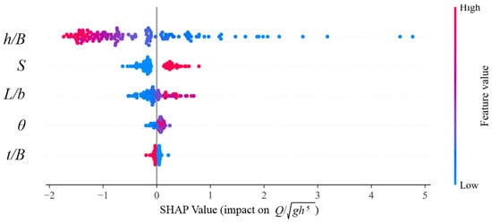
Figure 6. SHAP values (diagram on the top) and feature importance (diagram on the bottom) in predicting the dimensionless flow rate Q/√gh⁵.

Based on Figure 6, the analysis shows that the h/B feature has the most significant impact on predicting the dimensionless flow rate Q/√gh⁵. This feature exhibits very high SHAP values in most samples, with a positive direction, clearly indicating its key role in the model’s predictions. In other words, changes in the h/B value have a considerable effect on the model’s output, emphasizing the importance of this feature in the sensitivity analysis. The S feature also stands out as an influential factor in the predictions. Although its impact is less than that of h/B, the high dispersion of SHAP values suggests that it has a considerable influence on the prediction in certain samples. This dispersion indicates that S can play a varying role under different data conditions. The features L/b, θ, and t/B, while having less impact, still contribute to the model’s predictions. In particular, the SHAP values of these features are scattered in many samples, showing that their effects become noticeable under specific data conditions. This dispersion indicates that each of these features may have different effects on the model’s outcome in different scenarios.

In general, Figure 6 indicates that h/B is clearly the most significant factor in predicting the flow rate, and S is the second most significant factor. All the remaining features, including L/b, θ, and t/B, though being less significant, are vital to the prediction process. This analysis demonstrates the capability of the model in detecting intricate relations between features with precise prediction of results, and comments on the significance of utilizing comprehensible methods such as SHAP in tackling intricate problems.

Four metaheuristic algorithms (i.e., PSO, SSA, GA, and CMA-ES) were tested against each other for hyperparameter tuning in this work. Since minimization of computational cost was a concern, the initial test was performed on a base model, LightGBoost alone. Comparison was performed against the following measures: (i) Minimum RMSE as a measure of final accuracy, (ii) Mean and standard deviation of RMSE as measures of stability; (iii) Number of iterations and time to achieve 95% best performance as a measure of convergence speed; (iv) Computational cost (CPUh) as a measure of resource utilization.

Table 9 shows the relative performance of the four metaheuristic algorithms, and Figure 7 shows the convergence behavior of the algorithms.

Table 9. Comparison of metaheuristic algorithms for hyperparameter tuning of the LightGBoost model.

Algorithm	Best RMSE	Mean RMSE ± SD	Iterations to 95% Best	Time to 95% Best	CPUh
CMA-ES	0.154	0.156 ± 0.0017	85	42 min	4.58
SSA	0.155	0.156 ± 0.0013	68	37 min	4.08
PSO	0.159	0.160 ± 0.0019	90	44 min	4.42
GA	0.162	0.163 ± 0.0022	110	48 min	4.83

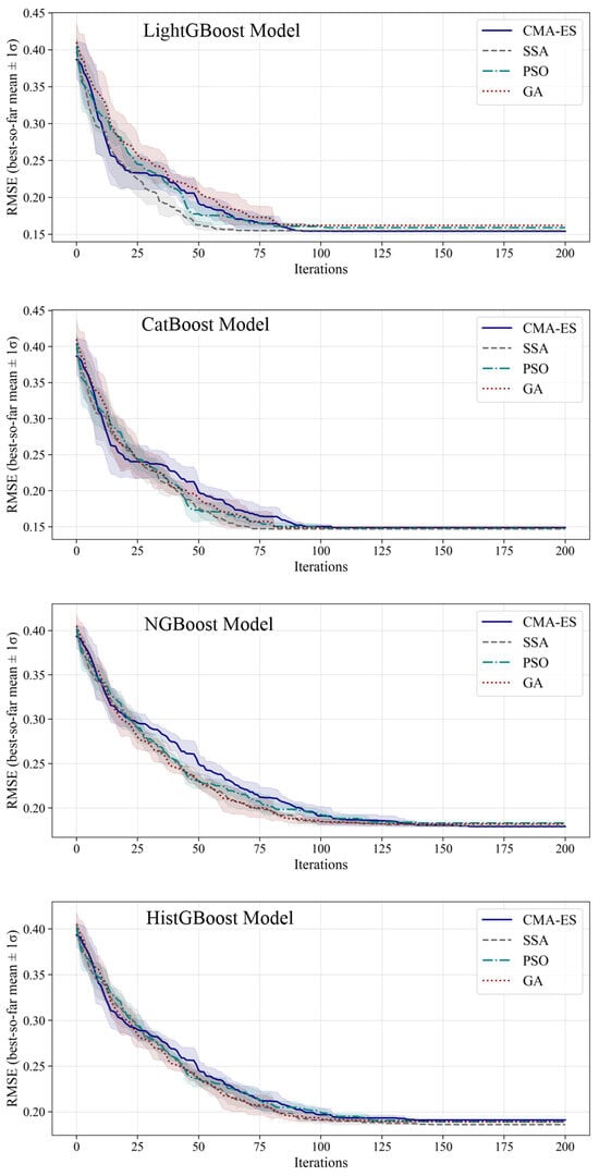
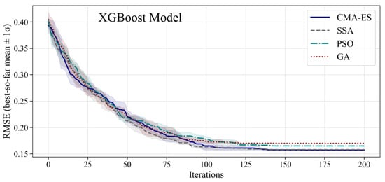
Figure 7. Convergence profiles of metaheuristic algorithms in hyperparameter tuning of the GB models.

Based on the results presented in Table 9, the CMA-ES achieved the lowest best RMSE (0.154). SSA provided more stable mean performance, reached 95% of the best result faster, and required the least computational cost. PSO and GA showed weaker performance in terms of both accuracy and resource consumption. Considering the time constraint of less than one hour and computational efficiency, SSA was selected as the most suitable algorithm for hyperparameter tuning of the GB models, as it offered a balanced trade-off between accuracy, speed, and computational cost.

The parameter settings of the four metaheuristic optimizers (CMA-ES, SSA, PSO, and GA) used to explore these ranges are reported in Table 10.

Table 10. Parameter settings of metaheuristic optimizers.

Algorithm	Parameter	Value	Algorithm	Parameter	Value
CMA-ES	Population size	30		Max. iterations	80
	Max. iterations	80		Inertia weight w	0.7
SSA	Population size	30		Cognitive coefficient c1	1.5
	Max. iterations	80		Social coefficient c2	1.5
	Producer fraction PD	0.20	GA	Population size	30
	Awareness probability AP	0.10		Max. generations	80
	Safety threshold ST	0.80		Crossover probability Pc	0.80
PSO	Population size	30		Mutation probability Pm	0.10

The main hyperparameters tuned for each GB model and their corresponding search ranges are summarized in Table 11.

Table 11. Hyperparameter tuning search ranges for the GB models.

Model	Hyperparameter	Search Range	Model	Hyperparameter	Search Range
HistGBoost	LR	0.01–0.25		L2R	1 × 10−3–10
	MI	100–1500		VB	−1–2
	MLN	5–63	NGBoost	LR	0.01–0.30
	ES	False–True		NE	100–1500
LightGBoost	LR	0.01–0.30		MBF	0.10–1.00
	NL	16–128		VE	−1–2
	MCS	5–100	XGBoost	LR	0.01–0.30
	VB	−1–2		MD	2–8
CatBoost	LR	0.01–0.30		MCW	1–10
	DP	2–10		VB	−1–2

The lower and upper bounds for each hyperparameter were selected by combining (i) commonly recommended ranges in the original implementations of the algorithms, (ii) values frequently adopted in previous hydrologic and hydraulic applications of tree-based ensemble methods, and (iii) preliminary trial runs aimed at avoiding severe underfitting (too few trees or overly strong regularization) and excessive overfitting or computational cost (very deep trees or extremely large ensembles). In Table 12, the optimized hyperparameters of the GB models tuned by SSA are presented.

Table 12. Optimized hyperparameters of GB models tuned by SSA.

Model		Model
HistGBoost-SSA	LR = 0.3		MCS = 11
	MI = 300		VB = −1
	MLN = 10	NGBoost-SSA	LR = 0.1
	ES = False		NE = 200
CatBoost-SSA	LR = 0.104		MBF = 0.228
	DP = 3		VE = 1
	L2R = 1.0	XGBoost-SSA	LR = 0.137
	VB = 1		MD = 7
LightGBoost-SSA	LR = 0.3		MCW = 9.707
	NL = 20		VB = 0

Next, the hybrid GB models were evaluated for estimating Q through the RTHG. Figure 8 shows scatter plots, residuals, and density distributions of the CatBoost-SSA model during training and testing stages. Table 13 presents the performance evaluation metrics of the CatBoost-SSA model for these stages.

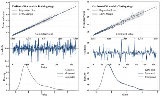
Figure 8. Scatter plots, residuals, and KDE distributions for the CatBoost-SSA model during the training and testing stages.

Table 13. Performance metrics of the CatBoost-SSA model during the training and testing stages.

Stage	R2	RMSE	MAE	MAPE	PBIAS
Training	0.999	0.039	0.029	1.324	−0.001
Testing	0.984	0.147	0.092	3.641	0.129

Based on the results from the experimentation of the CatBoost-SSA model during training and testing, the model performed adequately during the estimation of Q through RTHG. The model performed nearly perfect prediction during training. The R² value of 0.999 shows a very good fit with the actual values, validating the model’s ability to replicate the training set very well. Also, the extremely low values of 0.039 for RMSE and 0.029 for MAE are also in favor of the model being precise in its predictions. These also stood out in the scatter plot where points remain close to the regression line, indicating minimal difference between the actual and predicted values. Thus, the model was effective in learning the features of data and producing very good predictions when being trained. When tested, the model’s performance fell a little bit. R² decreased to 0.984, indicating that even though the model performs remarkably well, it had some problems with new data. This small deviation from the training period is expected because the model is now trained on unseen and new data. Also, the RMSE value (0.147) and MAE value (0.092) both increased, as would be the case with the natural errors that occur when a model is fitted to new data. All the other evaluation metrics also clearly show that the CatBoost-SSA model performs extremely well during the test period. MAPE rose from 1.324% at the training stage to 3.641% at the testing stage, which implies that at the testing stage, the prediction errors were marginally high. The value of PBIAS also rose to 0.129%, which implies a minor positive bias in the predictions at the testing stage. Residual analysis also shows that the model predictions are unbiased, as is evident from the plots of the residuals. During the training period, residuals were consistently spread about zero, meaning there is no systematic underprediction of the model. The feature was also exhibited during the testing period, though the residuals during the period were spread, which is the larger normal variance in the process of handling new data. Lastly, the KDE plots show how the calculated values mirror the measured values closely across the training period, which is a sign that the model is well calibrated. During the test period, while the distributions begin to deviate slightly, there is still a large similarity between the estimated and actual distributions, which reflects that the model is able to forecast the novel data with a good accuracy. Briefly, the CatBoost-SSA model was efficient during both the training and testing phases. The model’s high accuracy in the training stage and its still-acceptable performance on testing data emphasize its ability to simulate the complex flow rate dynamics through RTHG. These results highlight the effectiveness of using SSA for hyperparameter optimization in complex modeling tasks and demonstrate that combining these techniques can significantly improve prediction accuracy in sophisticated models.

Figure 9 presents scatter plots, residuals, and KDE distributions for the NGBoost-SSA model during training and testing stages. Table 14 summarizes the performance metrics of the NGBoost-SSA model for these stages.

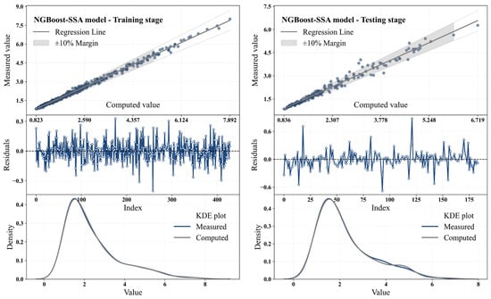
Figure 9. Scatter plots, residuals, and KDE distributions for NGBoost-SSA model at training and testing stages.

Table 14. Performance metrics of NGBoost-SSA model at training and testing stages.

Stage	R2	RMSE	MAE	MAPE	PBIAS
Training	0.995	0.10	0.076	3.406	0.049
Testing	0.976	0.18	0.118	4.880	0.311

The NGBoost-SSA model demonstrated excellent performance in both the training and testing stages in predicting Q through the RTHG. In the process of training, the model was able to obtain a value of R² equal to 0.995, which confirms that actual and predicted values have a perfect fit. The model was able to obtain low values for RMSE (0.10) and MAE (0.076), which confirm the validity of its predictions. The scatter plot also showed that data points were trending closely along the line of regression, confirming the model’s high predictability. Moreover, residual analysis indicated that the residuals lay randomly about zero and thus no sign of any sort of systematic bias was present. Throughout the test phase, even though performance did decline somewhat, the model retained excellent predictive ability. The R² metric fell to 0.976 but was still suggestive of close conformity with test data. RMSE went up to 0.18, and MAE to 0.118, a common result when the model is fed new, unseen data. MAPE also went up to 4.88%, a minimal rise in percentage error, but still within tolerable thresholds. During training, the model had an R² of 0.993, showing near-perfect correlation with the true values. The PBIAS values were minimal in the training stage (0.049%), indicating almost no bias in predictions, while in the testing stage, PBIAS increased to 0.311%, showing a slight positive bias, but still within a reasonable level. These small changes in bias are typical when models are tested on new data. Finally, residual and KDE analysis further supports the model’s effectiveness. In the training stage, the computed values closely aligned with the measured values, indicating a good fit. In the testing stage, although the distributions began to diverge slightly, they still showed reasonable alignment, confirming that the model can predict new data effectively. Overall, the NGBoost-SSA model performed well in both the training and testing stages. It demonstrated strong predictive capabilities for estimating Q through the RTHG and maintained good performance when exposed to new data.

Figure 10 shows scatter plots, residuals, and KDE distributions for the HistGBoost-SSA model during training and testing stages. Table 15 summarizes the performance metrics of the HistGBoost-SSA model for these stages.

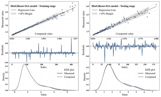
Figure 10. Scatter plots, residuals, and KDE distributions for the HistGBoost-SSA model during the training and testing stages.

Table 15. Performance metrics of HistGBoost-SSA model at training and testing stages.

Stage	R2	RMSE	MAE	MAPE	PBIAS
Training	0.993	0.116	0.044	1.494	0
Testing	0.974	0.186	0.112	4.498	0.406

The evaluation results of the HistGBoost-SSA model during both the training and testing stages demonstrate its excellent performance in predicting Q through the RTHG. In the training stage, the model achieved an R² value of 0.993, indicating a nearly perfect fit with the actual values. The same accuracy is also observed on the scatter plot, where dots are tightly bunched up near the regression line and clearly indicate that the model had accurately predicted values. Moreover, the RMSE of 0.116 and MAE of 0.044 also authenticate the accuracy of the model to reduce errors and predict closely to real values. Residual analysis also assured that the residuals were randomly scattered around zero, indicating that there was no systematic error in the model. The KDE plot also indicated that the estimated values were extremely close to the observed values, which confirms the strong performance of the model when trained. Throughout the test period, even when there was some deterioration in performance, the model still delivered acceptable outputs. The value of R² dropped to 0.974 but remained high, which also shows that the model still fits the test data extremely well. The RMSE increased to 0.186, and MAE to 0.112, which is a natural increase in errors as the model is being tested on new unseen data. MAPE also went up to 4.498%, showing a greater percentage of error in predictions compared to the training process. PBIAS rose to 0.406% in the testing phase, up from 0 in the training phase. This is a small positive bias in test predictions, though still in a good range. The HistGBoost-SSA model performed quite well overall in the training phase, and even when it suffered some slight loss of accuracy in the testing phase, it accurately predicted the flow rate through RTHG. These findings acknowledge the effective use of the SSA in hyperparameter optimization and predictive performance improvement of the models.

Figure 11 shows scatter plots, residuals, and KDE distributions for the XGBoost-SSA model at training and testing levels. Table 16 reports the related performance of the XGBoost-SSA model.

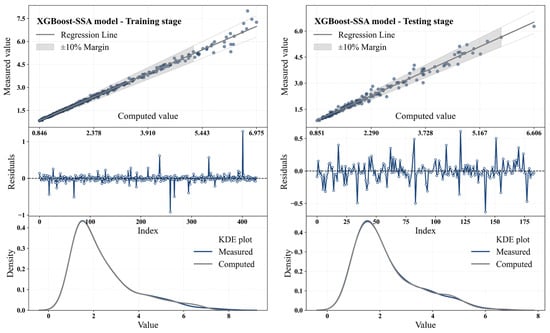
Figure 11. Scatter plots, residuals, and KDE distributions for the XGBoost-SSA model at the training and testing stages.

Table 16. Performance metrics of the XGBoost-SSA model at the training and testing stages.

Stage	R2	RMSE	MAE	MAPE	PBIAS
Training	0.993	0.114	0.052	1.836	−0.001
Testing	0.981	0.158	0.100	4.155	0.374

The XGBoost-SSA model showed exceptional performance in predicting Q through the RTHG during both the training and testing stages. In the training phase, the R² value of the model was 0.993, demonstrating a perfect fit of the model to actual data. The very small RMSE value of 0.114 and MAE value of 0.052 show that the predictions were very accurate with minimal amount of error involved. This accuracy is also evident from the scatter plot, since the data points are lying very close to the regression line, confirming the precision of the model while making predictions. The residual plot in the training period showed that the residuals were randomly varying around zero and there was no systematic bias. The KDE plot also confirmed the same by showing the predicted values were extremely close to the actual values, validating the excellent performance of the model. In the testing period, there was a dip in performance, but it was extremely slight. The R² also dropped to 0.981, having an extremely high correlation with the test data. RMSE rose to 0.158 and MAE to 0.100, both of which indicate a slight rise in errors when the model processed new data. Likewise, MAPE rose to 4.155%, which is higher compared to the training period but still low. PBIAS rose to 0.374% in the test phase from around 0 in the training phase. This represents a marginal positive prediction bias during the test phase, but this improvement is still within acceptable limits. The XGBoost-SSA model generally performed well during the training and testing phases. Despite slightly higher errors when tested, it was still able to make precise predictions of flow rate through the RTHG. This indicates the model’s capability to generalize new data extremely well and suggests the efficacy of applying SSA in hyperparameter tuning for complicated modeling tasks.

Scatter plots, residuals, and KDE distributions of the LightGBoost-SSA model in the training and testing phases are depicted in Figure 12. Table 17 summarizes the performance metrics of the LightGBoost-SSA model for these stages.

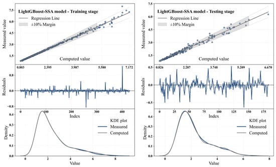
Figure 12. Scatter plots, residuals, and KDE distributions for the LightGBoost-SSA model at the training and testing stages.

Table 17. Performance metrics of the LightGBoost-SSA model at the training and testing stages.

Stage	R2	RMSE	MAE	MAPE	PBIAS
Training	0.995	0.099	0.037	1.226	0
Testing	0.982	0.155	0.103	4.389	0.618

The LightGBoost-SSA model demonstrated excellent performance in both the training and testing stages for predicting Q through the RTHG. In the training session, the model had an R² of 0.995, which is a very good data fit. The RMSE of 0.099 and MAE of 0.037 also show the accuracy of the model in making a flow rate prediction. This can also be seen from the scatter plot, where points are very close to the regression line, which shows the accuracy of the model while making predictions. Residual analysis indicated that the residuals were randomly distributed around zero, i.e., the model was free from any systematic bias. The KDE plot also indicated that the estimated values were very close to the actual values, verifying the robust behavior of the model during training. In the testing phase, the model was still reporting good results while dropping in performance. R² fell to 0.982, which is an indication of good agreement with the test data. The RMSE increased to 0.155, and MAE to 0.103, which is expected as the model is now being tested on new data. Similarly, MAPE rose to 4.389%, which is higher than in the training stage, but still within an acceptable range. PBIAS increased to 0.618% in the testing stage, compared to 0 in the training stage. This suggests a slight positive bias in the model’s predictions when tested on new data, which could be due to differences between the training and testing datasets. However, this value remains within an acceptable range. Overall, the LightGBoost-SSA model performed excellently in the training stage and, despite a slight increase in errors during testing, continued to provide accurate predictions of Q. These results highlight the effectiveness of using SSA for hyperparameter optimization and demonstrate the model’s capability to generalize well to unseen data.

For a more precise comparison and ranking of the hybrid GB models’ performance in predicting Q through the RTHG, Taylor diagrams were used at training and testing stages, as shown in Figure 13, providing a comprehensive and reliable evaluation of the models.

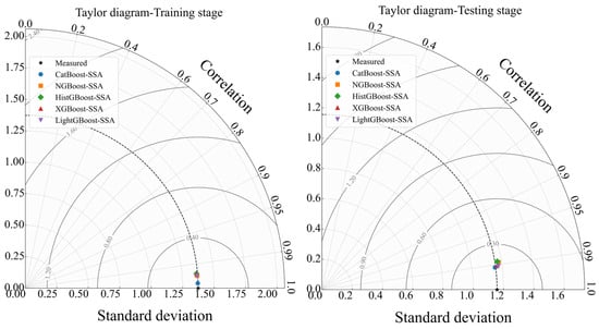
Figure 13. Taylor diagrams for comparing the performance of hybrid GB models in estimating Q through the RTHG at training and testing stages.

The analysis of the Taylor diagrams and c′ values based on Figure 13 demonstrates the overall quality of the hybrid models based on GB algorithms in predicting Q through the RTHG. At the training stage, all models exhibit performance very close to the observed data, as evidenced by the low c′ values and the proximity of the model points to the reference point on the Taylor diagram. Specifically, the model with the lowest c′ value of 0.0394, i.e., CatBoost-SSA, best fits the data and stands first. The LightGBoost-SSA model having a c′ value of 0.0988 ranks second, and the NGBoost-SSA model with a c′ value of 0.1002 ranks third. Their minimum values of c′ signify extremely negligible error in correctly estimating the flow, and their predictions closely follow the actual data. During the testing phase, the same trend of preserving accuracy is witnessed, with c′ values having increased to represent greater complexity in the test data and model generalization challenges. However, the best performance is still maintained by the CatBoost-SSA model with a c′ value of 0.1476, followed by the LightGBoost-SSA model with 0.1550 and the XGBoost-SSA model with 0.1579. The HistGBoost-SSA and NGBoost-SSA models rank lower because they possess higher c′ values. The Taylor diagrams indicate that the correlation between the predictions and observed data is very high for all models, clearly reflecting the reliability and overall accuracy of the models. Additionally, the standard deviations of the models are acceptably close to those of the observed data, indicating the models’ ability to simulate the variability in the data effectively.

To examine the absence of overfitting, the learning curves of the best-performing model (CatBoost-SSA) are presented in Figure 14.

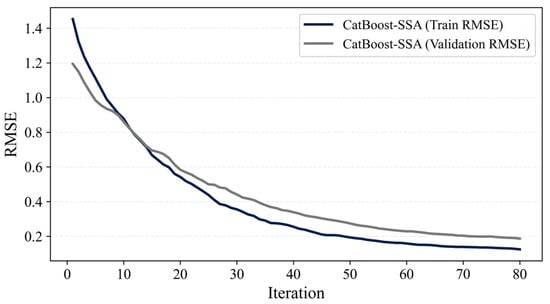
Figure 14. Learning curves of the CatBoost-SSA model.

The training and validation RMSE curves decrease smoothly and converge, indicating stable learning behavior without overfitting. Table 18 summarizes the five-fold cross-validation R² values for all SSA-based GB models, providing a comprehensive evaluation of their generalization consistency across folds. The 5-fold CV results reveal highly stable R² performance for all optimized GB models, confirming robust generalization and the absence of overfitting.

Table 18. Five-fold cross-validation R² values of the SSA-based GB models.

Model	F1	F2	F3	F4	F5	Mean R2
CatBoost-SSA	0.9988	0.9993	0.9991	0.9992	0.9995	0.9992
LightGBM-SSA	0.9950	0.9952	0.9947	0.9960	0.9949	0.9948
XGBoost-SSA	0.9928	0.9931	0.9932	0.9935	0.9927	0.9931
HistGBoost-SSA	0.9925	0.9930	0.9931	0.9933	0.9927	0.9928
NGBoost-SSA	0.9943	0.9948	0.9950	0.9953	0.9945	0.9947

In the following analysis, the focus is on evaluating whether the developed hybrid models exhibit physically plausible hydraulic behavior beyond the range of the laboratory data. Since Gradient Boosting models, and machine-learning approaches in general, lack inherent physical structure, they may generate non-physical responses under extrapolation. Therefore, using the best-performing model of this study, namely the CatBoost-SSA model, a set of physics-based sanity tests was conducted.

In these tests, the channel and gate geometry were fixed using representative mid-range values from the experimental dataset, including: channel width B = 0.25 m, length ratio L/b = 2.0, and thickness ratio t/B = 0.02. The depth ratio h/B was then varied over a uniform grid ranging from 0.05 to 1.05, representing an extension of approximately 10–15% beyond the experimental domain. For each depth value, three longitudinal slopes, S = 0 and 0.005, were considered, and the model output was subsequently predicted.

Figure 15 shows the results of the physics-based sanity checks performed for the CatBoost-SSA model under controlled extrapolation conditions. Panel (a) illustrates the predicted discharge Q as a function of h^3/2 for two longitudinal slopes (S = 0 and S = 0.005), demonstrating smooth, monotonic, and physically plausible behavior, with higher discharges observed for the larger slope. Panel (b) presents the variation in the dimensionless discharge Q/√gh⁵ versus the depth ratio h/B, where the predictions remain bounded, stable, and consistent with expected hydraulic trends across the extended depth range.

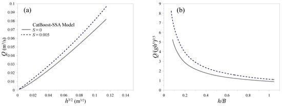
Figure 15. Physics-based sanity checks for the CatBoost-SSA model; (a) Q vs. h^3/2 and (b) Q/√gh⁵ vs. h/B.

Next, the uncertainty of the hybrid GB models in estimating Q through the RTHG is examined. In this regard, Figure 16 presents the CI values and R-Factor indices for the hybrid GB models, providing insight into the reliability and robustness of the predictions.

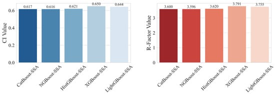
Figure 16. CI values and R-Factor indices for hybrid GB models estimating Q through RTHG.

According to Figure 16, the CI values and R-Factor indices indicate that all hybrid GB models exhibit comparable levels of uncertainty and reliability in estimating Q through the RTHG. The NGBoost-SSA model ranks lowest with the lowest CI (0.616) and R-Factor (3.596) values, indicating that it possesses the most confident and accurate predictions among the models that were considered, followed by CatBoost-SSA. The CI values of all the models are also closely similar, ranging from 0.616 to 0.650. This close proximity signals uniform levels of uncertainty across models with minimal variation in prediction accuracy. The same goes for R-Factor scores 3.596 to 3.791, signaling minimal variation in agreement between prediction and actual data. Since NGBoost-SSA is marginally better than others regarding CI and R-Factor, CatBoost-SSA and HistGBoost-SSA also have high accuracy and reliability. In contrast, XGBoost-SSA and LightGBoost-SSA have relatively higher CI and R-Factor scores, which reflect relatively higher uncertainty and deviance in their prediction. All in all, the research indicates that all the hybrid GB models offer good predictions, but NGBoost-SSA is slightly better at reducing uncertainty and enhancing prediction reliability. These findings support the use of these models, particularly NGBoost-SSA and CatBoost-SSA, for accurate and dependable flow rate estimation through the RTHG in engineering applications.

Figure 17 illustrates the observed data and predicted Q values with 95% confidence bands for the evaluated hybrid GB models, demonstrating the uncertainty bounds of the model predictions across the samples.

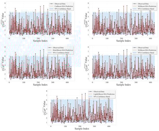
Figure 17. Observed data and predicted Q values with 95% confidence bands for the evaluated hybrid GB models.

The results depicted in Figure 17 reveal that the observed data and predicted Q values, along with the 95% confidence bands, effectively illustrate the uncertainty bounds of the hybrid GB models’ predictions across the sample indices. The bands of confidence provide a graphical representation of the area where the actual flow values should fall with 95% probability, giving a simple idea of the reliability of predictability of each model. For all models, the fitted values plot in line with the observed data fairly well, suggesting that all models can represent the overall dynamics of flow fairly well. Particularly, the confidence bands of CatBoost-SSA and NGBoost-SSA models are relatively narrower and closer to observed values, indicating smaller prediction uncertainty and greater reliability. All other models, though still of reasonable fit, have relatively wider confidence bands in some of the sample points, indicating greater uncertainty at these points. In general, Figure 17 validates that the hybrid GB models make precise predictions with measurable uncertainty, and emphasizes the higher stability and assurance of models such as CatBoost-SSA and NGBoost-SSA for predicting flow rates via RTHG.

To complement the bootstrap-derived confidence intervals, the native probabilistic output of NGBoost-SSA was evaluated. As illustrated in Figure 18, the mean width of NGBoost’s 95% prediction intervals on the test set is only 0.26 in terms of Q/√gh⁵, with a median width of 0.24. When normalized by the maximum observed value, this corresponds to a CI-like index of 0.041, which is markedly smaller than the bootstrap-based CI value of 0.616. This sharp reduction demonstrates that NGBoost-SSA produces considerably narrower yet well-covering predictive intervals, capturing most of the aleatoric variability with only limited epistemic spread. Overall, the results presented in Figure 18 confirm that NGBoost-SSA exhibits the lowest total predictive uncertainty among all SSA-optimized GBMs evaluated in this study.

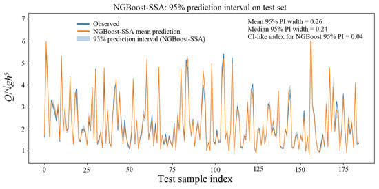
Figure 18. 95% prediction intervals generated by the NGBoost-SSA model on the test set, along with observed values and mean predictions.

Empirical models based on regression analysis are widely utilized tools in the investigation of hydraulic phenomena and are commonly applied in the design of spillways and hydraulic gates. Additionally, empirical models are employed for RTHG. Among these, one of the most accurate relationships is Equation (5), which has been derived from experimental data used in this article [3].

$${\displaystyle \frac{Q}{\sqrt{g{B}^5}}}=\left(0.547-36S\right){\left({\displaystyle \frac{h}{B}}\right)}^{1.82-8S}{\left({\displaystyle \frac{b}{B}}\right)}^{-0.13-40S}{\left({\displaystyle \frac{t}{B}}\right)}^{-0.12-23.3S}{\left({\displaystyle \frac{L}{B}}\right)}^{-0.1}$$

(5)

In this study, to demonstrate the superior performance of the machine learning models, their results are compared with those of the empirical model. Equation (5) defines the dimensionless parameter Q/√gB⁵, while the intelligent models presented herein determine the value of the parameter Q/√gh⁵. For a more accurate comparison, the value of Q is first calculated using Equation (5), and subsequently, the dimensionless parameter Q/√gh⁵ is computed. These calculated values are then compared with the observed values, and statistical functions along with model evaluation indices are used to assess the performance of the models.

Scatter plots, residuals, and KDE distributions computed by Equation (5) in the testing dataset are presented in Figure 19. Table 19 also summarizes the performance metrics of the empirical model.

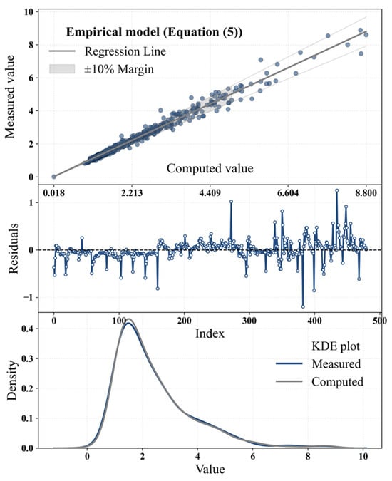
Figure 19. Scatter plots, residuals, and KDE distributions of the empirical model computed by Equation (5) in the testing dataset.

Table 19. Performance metrics of the empirical model in the testing dataset.

Equation (5)	R2	RMSE	MAE	MAPE	PBIAS
	0.944	0.255	0.174	5.570	−0.122

As illustrated in Figure 19 and summarized in Table 19, the empirical model also delivers acceptable accuracy, showing a reasonable alignment between the computed and observed values in the testing dataset. However, despite its satisfactory performance, the level of precision required for design-oriented hydraulic applications typically demands models with higher predictive capability. In this regard, the hybrid gradient boosting models developed in this study provide markedly superior accuracy and reduced error levels, making them more suitable than the empirical formulation for engineering design and reliable flow estimation through RTHGs.

4. Discussion

The experimental data utilized in the current work were rigorously tested prior to model training and evaluation. The dataset was initially collected from a set of well-regulated laboratory experiments under steady flow conditions using precision instruments to quantify the flow rate, head, and gate angle. The repeatability and reproducibility of the measurement were attained by comparing repeated runs and applying the Local Outlier Factor (LOF) algorithm to detect and eliminate any outlier point. The experiments were conducted in a comparatively large flume with Reynolds numbers being high enough to provide turbulent flow; hence, scale effects can be confidently neglected. In addition, normalization and dimensional analysis were performed to reduce any remaining effect of scale variability.

In as far as the capacity of the models to identify scale-dependent data is concerned, the implemented ensemble learning algorithms (CatBoost, NGBoost, XGBoost, LightGBM, and HistGBoost) have the innate capacity to identify complex nonlinear relationships between input and output variables. Assuming they are trained with clean and uniform data, they can identify anomalous or uncorrelated patterns, which would appear as low SHAP importance or high residuals. However, since the data available had already been gathered under laboratory conditions without zero-order scale effects, this problem did not have much impact on the present study.

Even though the main aim of this work was to create robust predictive models for estimating the flow rate, the derived models can also be written in empirical-type equation form. The models for simple correlations between dimensionless discharge and the most significant, most impacting parameters (e.g., h/b, b/B, θ, and S) can be obtained by symbolic regression or surrogate modeling methods based on feature importance ranking and SHAP analysis. This may be a fruitful line of future research to create general-gauge discharge formulas that capture the reality of data-based models with the parsimony of empirical models.

Lastly, the physical consistency of the created models was checked by sensitivity and interpretability tests. The sign and magnitude of the SHAP values ensured that the computed behavior of the models complies with the basic hydraulic principles—higher upstream head ratio or gate opening results in more discharge, whereas a higher gate angle or bed slope reduces it. This conformity of the physical understanding with model predictions reflects that not only are machine learning models learned correctly but also physically consistent in the explored domain.

To clarify the applicability of the proposed SSA-GBM models beyond the laboratory conditions, the hydraulic regime of the experimental dataset was analyzed, and the scaling limitations were explicitly considered. Although all measurements were obtained from a single laboratory flume, the predictor variables were defined in dimensionless form (h/B, L/b, t/B, S, and θ), which are inherently scale-independent and commonly used in hydraulic similitude. Reynolds numbers in the experiments ranged from 4.12 × 10³ to 2.97 × 10⁵, all above the classical laminar–turbulent transition and thus completely representative of predominantly turbulent flow conditions. The Froude numbers were in the range of 0.014 to 1.34; hence, most runs were subcritical, with a very small fraction of them approaching critical flow. SSA-GBM models are expected to retain their validity for field applications operating under similar hydraulic regimes. For practical applications, Re ≥ 1 × 10⁴ and 0.02 < Fr < 1.0 are recommended to limit viscous and scale effects and also to avoid near-critical instabilities. It is also important to realize that real canals may have additional complexities due to much larger aspect ratios, greater three-dimensionality, sediment load, and variable roughness-all absent in the laboratory configuration and which might require added calibration in the field.

In addition to aleatoric uncertainty, which arises from the intrinsic variability of the measured discharge data and is quantified in this study through bootstrap confidence intervals and the R-Factor values, the models are also subject to epistemic uncertainty. This second component originates from the structure of the gradient-boosting models themselves, the limited range of the experimental parameter space, and the fact that all observations were collected within a single laboratory flume. These structural and model-based limitations imply that the learned response surfaces may not fully represent all possible hydraulic conditions beyond the tested combinations of h/B, L/b, t/B, and S. Therefore, epistemic uncertainty is inherently higher for models with greater structural complexity or weaker robustness. This distinction is especially important when evaluating the comparative reliability of the SSA-optimized GBMs.

The SHAP analysis shows that the depth ratio h/B is the most influential parameter in predicting the discharge (Q/√gh⁵). This result is fully consistent with hydraulic theory and with previous analytical studies on top-hinged gates. Physically, h/B directly controls the upstream specific energy and the magnitude of the hydrostatic force acting on the gate. As a result, even small increases in upstream depth significantly increase the opening beneath the gate, leading to a noticeable rise in discharge. This strong dependence matches the large exponents associated with h/B in classical power-law discharge relations. The channel slope S appears as the second most influential parameter. Although the tested slopes are small, variations in S modify the energy grade line, the approach velocity distribution, and the upstream pressure field. Previous laboratory results have also shown that using discharge equations from horizontal channels in sloping channels can lead to considerable errors, which confirms that slope effects must be accounted for. The importance assigned to S by the machine-learning models is therefore consistent with fundamental hydraulic behavior. In comparison, geometric parameters such as L/b, t/B, and θ show moderate but still meaningful impacts. Their lower influence agrees with earlier experimental findings, where these parameters were associated with small exponents or could sometimes be neglected without loss of accuracy. Nonetheless, the ML models correctly capture their secondary role in adjusting the moment balance and the detailed geometry of the opening beneath the gate.

At high discharges and velocities, several hydraulic mechanisms can explain the increased scatter and larger prediction errors. As the flow accelerates beneath the top-hinged gate, the Reynolds number and turbulence intensity rise, and the flow in the contraction region becomes more strongly three-dimensional. This can promote separation, local vortices, and secondary currents, especially for larger width ratios and mild channel slopes. Under these conditions, the actual pressure distribution and effective contraction beneath the gate may deviate from the simplified quasi-two-dimensional behavior implicitly assumed in the dimensional analysis. In addition, free-surface fluctuations and rapid variations in the under-gate jet make it more difficult to obtain accurate measurements of upstream depth, gate angle, and discharge at high velocities, which increases measurement uncertainty in exactly the range where the flow is most energetic. These highly nonlinear and partially three-dimensional effects pose a challenge for the ML models, because they typically occur in the upper tail of the dataset where the number of observations is relatively limited and the relationship between the input parameters and discharge becomes more complex and less smooth. In these setups, even a flexible ensemble learning model may have a hard time capturing the physical behavior fully and may be even more prone to errors due to noisy/biased learning data. Some potential solution ideas include selective data augmentation with greater numbers of high-velocity runs within the existing experiment setup, and implementing some form of available physical insights directly within the learning process itself. This would include inputs such as those related to the derived numerical values for Froude numbers and energy head, with constraints related only to some straightforward physical notions, such as a monotonically non-decreasing discharge with a given increase in depth, among other possibilities related directly to water flow principles.

In order to position the present work within the broader context of flow-measurement research, it is useful to compare our results with previous studies on weirs, sluice gates, and hinged-gate devices. Classical rating equations for sharp-crested weirs and sluice gates typically express discharge as a power-law function of upstream depth and a limited set of geometric parameters, with calibration coefficients that must be re-fitted whenever the structure geometry or flow regime changes. Similar dimensionless discharge relations have been proposed for circular and rectangular hinged gates, including the base experimental study used in this work, where the influence of depth, width ratio, gate length and slope is condensed into a small number of Π-groups and power-law exponents. Our hybrid ML models reproduce the same dominant hydraulic trends reported in these studies: discharge increases monotonically with upstream depth and is sensitive to channel slope and width ratio, while the effects of thickness and gate length remain secondary. At the same time, the SSA-tuned gradient boosting and NGBoost models achieve substantially lower prediction errors than the original empirical relations over the same experimental dataset and are able to accommodate the combined effects of multiple geometric and hydraulic parameters without requiring separate calibration for each configuration. Moreover, unlike traditional deterministic formulas, the NGBoost-SSA model provides full predictive distributions and allows confidence intervals and R-Factor based uncertainty metrics to be computed directly from the model outputs, which is rarely available for conventional weir or gate equations. From a methodological perspective, the main scientific contribution of this study is to demonstrate a coherent hybrid framework that combines: (i) dimensional analysis and ANOVA to define physically meaningful input features, (ii) local outlier detection and careful data preprocessing, (iii) SSA-based global hyperparameter optimization of several state-of-the-art gradient boosting algorithms, and (iv) model-agnostic explainability (SHAP) and uncertainty analysis for a practical flow-measurement device. This integrated approach goes beyond previous work on weirs and gates that relied solely on empirical regression or single black-box models, and shows that machine learning can be used not only to improve accuracy, but also to enhance physical interpretability and quantify predictive uncertainty for hydraulic structures.

5. Conclusions

The accurate estimation of flow rates (Q) through structures such as the Rectangular Top-Hinged Gate (RTHG) is a critical aspect of hydraulic engineering, as it directly impacts the efficiency and safety of water management systems. This study aimed to improve the prediction of flow rates through the RTHG by utilizing hybrid models based on gradient boosting algorithms, which offer advanced capabilities for handling complex, nonlinear relationships in hydraulic data. The primary objective was to develop an accurate model for estimating Q through the RTHG using hybrid models, including Categorical Boosting (CatBoost), Natural Gradient Boosting (NGBoost), Histogram-based Gradient Boosting (HistGBoost), Extreme Gradient Boosting (XGBoost), and Light Gradient Boosting (LightGBoost). One of the essential factors in developing artificial intelligence models is the accurate and proper tuning of their hyperparameters. Therefore, four powerful metaheuristic algorithms—Covariance Matrix Adaptation Evolution Strategy (CMA-ES), Sparrow Search Algorithm (SSA), Particle Swarm Optimization (PSO), and Genetic Algorithm (GA)—were evaluated and compared for hyperparameter tuning, using LightGBoost as the baseline model. An assessment of error metrics, convergence speed, stability, and computational cost revealed that SSA achieved the best performance for the hyperparameter optimization of GB models. Consequently, hybrid models combining GB algorithms with SSA were developed to predict Q through RTHGs.

Outlier removal was carried out using the Local Outlier Factor (LOF) algorithm, and data normalization was achieved through Z-score normalization. In order to identify the dimensionless independent parameters that significantly influence Q predictions, dimensional analysis and analysis of variance (ANOVA) were performed. The dataset was divided into a training set (70%) and a testing set (30%) to ensure the robustness of the models. The performance of the models was evaluated using various metrics, including Coefficient of Determination (R²), Root Mean Square Error (RMSE), Mean Absolute Error (MAE), Mean Absolute Percentage Error (MAPE), and Percent Bias (PBIAS). Additionally, model comparison and ranking were conducted using the Taylor Diagram, and sensitivity analysis was performed through the SHAP method. The uncertainty in model predictions was quantified through Confidence Interval (CI) and R-Factor indices.

Based on the obtained results, all hybrid gradient boosting models demonstrated high accuracy in predicting Q through the RTHG during both training and testing phases. Among them, CatBoost-SSA achieved the highest performance, with an R² of 0.999 during training and 0.984 during testing, indicating its superior ability to model complex Q behavior with minimal error. The low values of RMSE (0.147) and MAE (0.092) in the testing phase confirm the robustness and generalizability of this model. NGBoost-SSA also showed strong performance with reliable predictions and the lowest uncertainty, as indicated by its confidence interval (CI = 0.616) and R-Factor (3.596), suggesting its predictions were the most consistent and trustworthy across different scenarios. Additionally, LightGBoost-SSA, XGBoost-SSA, and HistGBoost-SSA provided competitive results, with R² values above 0.97 in the testing phase, though they exhibited slightly higher levels of uncertainty compared to CatBoost and NGBoost.

SHAP analysis confirmed that the most influential parameter in predicting Q was h/B (upstream water depth to channel width ratio), followed by S (channel slope). These findings emphasize the importance of these physical parameters in Q modeling and highlight the interpretability of the machine learning approach used. Furthermore, the Taylor diagram analysis ranked CatBoost-SSA as the top-performing model, followed closely by LightGBoost-SSA and NGBoost-SSA, reinforcing the conclusion that these hybrid models are effective for complex hydraulic modeling tasks.

In conclusion, the integration of SSA with gradient boosting models not only enhanced prediction accuracy but also reduced uncertainty in modeling outcomes. This hybrid approach presents a promising tool for hydraulic engineers aiming to optimize the operation and design of gated structures such as RTHGs.

Limitations of the present study. Although the novel hybrid boosting models exhibited excellent predictive power and physical reasonability, several limitations should be mentioned. First, the dataset in the current study was measured in controlled laboratory settings and may not be fully representative of field-scale hydraulic behavior. Second, the models were trained and validated on a finite range of geometric and hydraulic parameters; thus, extrapolation beyond this range should be taken with caution. Thirdly, hyperparameter tuning was carried out with respect to one objective function (RMSE), and multi-objective optimization can be employed for improving model generalization. Finally, future studies are encouraged to incorporate larger and more diverse datasets, e.g., prototype-scale measurements, for enhancing the developed models’ robustness and applicability.

References

- Rajaratnam, N.; Subramanya, K. Flow equation for the sluice gate. J. Irrig. Drain. Div. 1967, 93, 167–186. [Google Scholar] [CrossRef]
- Daneshfaraz, R.; Ghahramanzadeh, A.; Ghaderi, A.; Joudi, A.R.; Abraham, J. Investigation of the effect of edge shape on characteristics of flow under vertical gates. J. Am. Water Work. Assoc. 2016, 108, E425–E432. [Google Scholar] [CrossRef]
- Gorgin, F.; Vatankhah, A.R. Rectangular top-hinged plate as portable flow measuring device. Water Supply 2022, 22, 8637–8658. [Google Scholar] [CrossRef]
- Forster, J.W. Discussion on “Hydraulic jump at an abrupt drop” by Walter L. Moore and Carl W. Morgan. Trans. Am. Soc. Civ. Eng. 1959, 124, 519–521. [Google Scholar] [CrossRef]
- Rajaratnam, N.; Subramanya, K. Flow immediately below submerged sluice gate. J. Hydraul. Div. 1967, 93, 57–77. [Google Scholar] [CrossRef]
- Ramamurthy, A.S.; Pani, B.S.; Subramanya, K. Sluice gates with high discharge coefficients. J. Irrig. Drain. Div. 1978, 104, 437–441. [Google Scholar] [CrossRef]
- Burrows, R. The hydraulic characteristics of hinged flap gates. In Hydraulic Design in Water Resources Engineering: Land Drainage, 1st ed.; Smith, K.V.H., Rycroft, D.W., Eds.; Springer: Berlin/Heidelberg, Germany, 1986; pp. 271–280. [Google Scholar]
- Burrows, R.; Ockleston, G.A.; Ali, K.H.M. Flow estimation from flap-gate monitoring. Water Environ. J. 1997, 11, 346–356. [Google Scholar] [CrossRef]
- Swamee, P.K. Sluice-gate discharge equations. J. Irrig. Drain. Eng. 1992, 118, 56–60. [Google Scholar] [CrossRef]
- Raemy, F.; Hager, W.H. Hydraulic level control by hinged flap gate. Proc. Inst. Civ. Eng. Marit. Energy. 1998, 130, 95–103. [Google Scholar] [CrossRef]
- Swamee, P.K.; Pathak, S.K.; Mansoor, T.; Ojha, C.S.P. Discharge characteristics of skew sluice gates. J. Irrig. Drain. Eng. 2000, 126, 328–334. [Google Scholar] [CrossRef]
- Litrico, X.; Belaud, G.; Baume, J.-P.; Ribot-Bruno, J. Hydraulic modeling of an automatic upstream water-level control gate. J. Irrig. Drain. Eng. 2005, 131, 176–189. [Google Scholar] [CrossRef]
- Lozano, D.; Mateos, L.; Merkley, G.P.; Clemmens, A.J. Field calibration of submerged sluice gates in irrigation canals. J. Irrig. Drain. Eng. 2009, 135, 763–772. [Google Scholar] [CrossRef]
- Belaud, G.; Cassan, L.; Baume, J.-P. Calculation of contraction coefficient under sluice gates and application to discharge measurements. J. Hydraul. Eng. 2009, 135, 1086–1091. [Google Scholar] [CrossRef]
- Vatankhah, A.R.; Ghaderinia, H. Semi-circular flap gate as a flow metering structure in circular channels. Flow Meas. Instrum. 2018, 64, 28–38. [Google Scholar] [CrossRef]
- Salmasi, F.; Nouri, M.; Sihag, P.; Abraham, J. Application of SVM, ANN, GRNN, RF, GP and RT models for predicting discharge coefficients of oblique sluice gates using experimental data. Water Supply 2021, 21, 232–248. [Google Scholar] [CrossRef]
- El Bilali, A.; Taleb, A. A novel approach for predicting peak flow from breached dam: Coupling Monte Carlo simulation, hydrodynamic model, and an interpretable XGBoost model. Water Resour. Manag. 2025, 39, 1177–1194. [Google Scholar] [CrossRef]
- Weekaew, J.; Suksuwan, N.; Baylar, A.; Ditthakit, P. Harnessing machine learning models to predict flow regimes over stepped spillways. Eng. Technol. Appl. Sci. Res. 2025, 15, 23721–23728. [Google Scholar] [CrossRef]
- Azma, A.; Sadrabadi, M.T.; Liu, Y.; Azma, M.; Zhang, D.; Cao, Z.; Li, Z. Boosting ensembles for estimation of discharge coefficient and through flow discharge in broad-crested gabion weirs. Appl. Water Sci. 2023, 13, 45. [Google Scholar] [CrossRef]
- Asgharzadeh-Bonab, A.; Bijanvand, S.; Parsaie, A.; Afaridegan, E. Machine learning-based estimation of discharge coefficient for semicircular labyrinth weirs. Sci. Rep. 2025, 15, 33002. [Google Scholar] [CrossRef]
- Belaabed, F.; Arabet, L.; Goudjil, K.; Ouamane, A. Optimized machine learning models for accurate prediction of the discharge coefficient in hydraulic weirs. J. Hydrol. Hydromech. 2025, 73, 295–309. [Google Scholar] [CrossRef]
- Bansal, N.; Singh, D.; Kumar, M. Computation of energy across the type-C piano key weir using gene expression programming and extreme gradient boosting (XGBoost) algorithm. Energy Rep. 2023, 9, 310–321. [Google Scholar] [CrossRef]
- Chooplou, A.C.; Kahrizi, E.; Fathi, A.; Ghodsian, M.; Latifi, M. Baffle-enhanced scour mitigation in rectangular and trapezoidal Piano Key Weirs: An experimental and machine learning investigation. Water 2024, 16, 2133. [Google Scholar] [CrossRef]
- Afaridegan, E.; Fatahi-Alkouhi, R.; Khalilian, S.; Moradi-Eshgafti, A.; Amanian, N. Enhanced energy dissipation prediction in modified semi-cylindrical weirs using machine learning techniques. Model. Earth Syst. Environ. 2025, 11, 131. [Google Scholar] [CrossRef]
- Dhar, M.; Sapkota, S.C.; Saha, P.; Arora, S. Evaluating discharge coefficient of rectangular sharp crested weirs using machine learning models. Water Resour. Manag. 2025, 39, 4151–4171. [Google Scholar] [CrossRef]
- Shirvan, S.H.; Pirzadeh, B.; Rajaei, S.H.; Bejestan, M.S. Multi-approaches evaluation for prediction of discharge coefficient of porous broad-crested weirs under upstream partial blockage. Iran J. Sci. Technol. Trans. Civ. Eng. 2025, 49, 4913–4925. [Google Scholar] [CrossRef]
- Bijanvand, S.; Asgharzadeh-Bonab, A.; Parsaie, A.; Afaridegan, E. Enhanced prediction of discharge coefficients in Harmonic Plan Circular Weirs using advanced machine learning and ensemble techniques. Flow Meas. Instrum. 2025, 102, 102812. [Google Scholar] [CrossRef]
- Afaridegan, E.; Amanian, N.; Goodarzi, M.R. Hybrid machine learning models for discharge coefficient prediction in hydrofoil-crested stepped spillways. Arch. Comput. Methods Eng. 2025, 32, 4413–4445. [Google Scholar] [CrossRef]
- Afaridegan, E.; Amanian, N.; Parsaie, A. Hydraulic performance of hydrofoil-crested stepped spillways: Air inception point and discharge coefficient. J. Appl. Water Eng. Res. 2025, 13, 169–185. [Google Scholar] [CrossRef]
- Cheng, Z.; Zou, C.; Dong, J. Outlier detection using isolation forest and local outlier factor. In Proceedings of the Conference on Research in Adaptive and Convergent Systems (RACS’19), Chongqing, China, 24–27 September 2019. [Google Scholar]
- Guryanov, A. Histogram-based algorithm for building gradient boosting ensembles of piecewise linear decision tree. In Analysis of Images, Social Networks and Texts; van der Aalst, W.M.P., Batagelj, V., Ignatov, D.I., Khachay, M., Kuskova, V., Kutuzov, A., Kuznetsov, S.O., Lomazova, I.A., Loukachevitch, N., Napoli, A., et al., Eds.; Springer: Cham, Switzerland, 2019; pp. 39–50. [Google Scholar]
- Dorogush, A.V.; Ershov, V.; Gulin, A. CatBoost: Gradient boosting with categorical features support. arXiv 2018, arXiv:1810.11363. [Google Scholar] [CrossRef]
- Oram, E.; Dash, P.B.; Naik, B. Light-gradient boosting machine for identification of osteosarcoma cell type from histological features. In Computational Intelligence in Cancer Diagnosis, 1st ed.; Nayak, J., Pelusi, D., Naik, B., Mishra, M., Muhammad, K., Al-Dabass, D., Eds.; Academic Press: New York, NY, USA, 2022; pp. 289–303. [Google Scholar]
- Duan, T.; Avati, A.; Ding, D.Y.; Thai, K.K.; Basu, S.; Ng, A.Y.; Schuler, A. NGBoost: Natural gradient boosting for probabilistic prediction. arXiv 2020, arXiv:1910.03225. [Google Scholar] [CrossRef]
- Moradi-Eshgafti, A.; Shahrokhi, S.; Yousefi-Kebria, A.; Nejatipour, P.; Afaridegan, E.; Ghannad, A. Assessment of accuracy and uncertainty in metaheuristic-optimized state-of-the-art AI models for predicting energy dissipation in streamlined stepped spillways. Multiscale Multidiscip Model. Exp. Des. 2025, 9, 24. [Google Scholar] [CrossRef]
- Chen, T.; He, T.; Benesty, M.; Khotilovich, V.; Tang, Y.; Cho, H.; Chen, K.; Mitchell, R.; Cano, I.; Zhou, T. XGBoost: Extreme Gradient Boosting; R Package Version 0.4-2; Scientific Research Publishing Inc.: Irvine, CA, USA, 2015; pp. 1–4. [Google Scholar]
- Afaridegan, E.; Fatahi-Alkouhi, R.; Azarm, P.; Amanian, N. Enhanced prediction of discharge coefficient in sharp-edged width constrictions using a novel hybrid SVR-IWOA and machine learning models. J. Hydrol. 2025, 657, 133103. [Google Scholar] [CrossRef]
- Hansen, N.; Müller, S.D.; Koumoutsakos, P. Reducing the time complexity of the derandomized evolution strategy with covariance matrix adaptation (CMA-ES). Evol. Comput. 2003, 11, 1–18. [Google Scholar] [CrossRef] [PubMed]
- Xue, J.; Shen, B. A novel swarm intelligence optimization approach: Sparrow search algorithm. Syst. Sci. Control Eng. 2020, 8, 22–34. [Google Scholar] [CrossRef]
- Kennedy, J.; Eberhart, R. Particle swarm optimization. In Proceedings of ICNN’95—International Conference on Neural Networks, Perth, WA, Australia, 27 November–1 December 1995. [Google Scholar]
- Goldberg, D.E. Genetic Algorithms in Search, Optimization, and Machine Learning; Addison-Wesley Publishing Company, Inc.: Menlo Park, CA, USA, 1989. [Google Scholar]
- Antwarg, L.; Miller, R.M.; Shapira, B.; Rokach, L. Explaining anomalies detected by autoencoders using Shapley Additive Explanations. Expert Syst. Appl. 2021, 186, 115736. [Google Scholar] [CrossRef]
- Shamsi, M.; Darian, J.T.; Afkhamipour, M. Assessment of mass transfer performance using the two-film theory and surrogate models for intensified CO2 capture process by amine solutions in rotating packed beds. Chem. Eng. Process. Intensif. 2025, 208, 110080. [Google Scholar] [CrossRef]
- Shahandashty, B.F.; Fallah, N.; Shamsi, M.; Nasernejad, B.; Afkhamipour, M. Evaluation of enhanced chemical coagulation method for a case study on colloidal liquid particle in wastewater treatment: Statistical optimization analysis and implementation of machine learning. J. Environ. Manag. 2024, 370, 122345. [Google Scholar] [CrossRef]
- Taylor, K.E. Summarizing multiple aspects of model performance in a single diagram. J. Geophys. Res. Atmos. 2001, 106, 7183–7192. [Google Scholar] [CrossRef]
- Efron, B.; Tibshirani, R.J. An Introduction to the Bootstrap; CRC Press LLC: Boca Raton, FL, USA, 1998. [Google Scholar]
- Yu, B.; Hashim, G.M.; Eusof, Z. Estimating the R-factor with limited rainfall data: A case study from Peninsular Malaysia. J. Soil Water Conserv. 2001, 56, 101–105. [Google Scholar] [CrossRef]
Disclaimer/Publisher’s Note: The statements, opinions and data contained in all publications are solely those of the individual author(s) and contributor(s) and not of MDPI and/or the editor(s). MDPI and/or the editor(s) disclaim responsibility for any injury to people or property resulting from any ideas, methods, instructions or products referred to in the content. |
© 2025 by the authors. Licensee MDPI, Basel, Switzerland. This article is an open access article distributed under the terms and conditions of the Creative Commons Attribution (CC BY) license (https://creativecommons.org/licenses/by/4.0/).