Application of a Heuristic Model (PSO—Particle Swarm Optimization) for Optimizing Surface Water Allocation in the Machángara River Basin, Ecuador

Abstract

Efficient surface water allocation in reservoir-equipped basins is essential for balancing competing demands within the Water–Energy–Food (WEF) nexus. This study investigated the applicability of Particle Swarm Optimization (PSO) for optimizing water distribution in the Machángara River Basin, Ecuador; a complex, constraint-rich hydrological system. Implemented via the Pymoo package in Python, the PSO model was evaluated across calibration, validation, and execution phases, and benchmarked against exact methods, including Linear Programming (LP) and Mixed Integer Linear Programming (MILP). The results revealed that standard PSO struggled to satisfy equality constraints and yielded suboptimal solutions, with elevated penalty costs. Despite incorporating MILP-inspired encoding and repair functions, the algorithm failed to identify feasible solutions that met operational requirements. The execution phase, which includes reservoir construction decisions, resulted in a total penalty exceeding EUR 164.95 billion, with no improvement observed from adding reservoirs. Comparative analysis confirmed that LP and MILP outperformed PSO in constraint compliance and penalty minimization. Nonetheless, the study contributes a reproducible implementation framework and a comprehensive benchmarking strategy, including synthetic test functions, performance metrics, and diagnostic visualizations. These tools can facilitate systematic evaluation of PSO’s behavior in high-dimensional, nonlinear environments and provide a foundation for future hybrid or adaptive heuristic models. The findings underscore the limitations of standard PSO in hydrological optimization but also highlight its potential when enhanced through hybridization. Future research should explore PSO variants that integrate exact solvers, adaptive control mechanisms, or cooperative search strategies to improve feasibility and convergence. This work advances the methodological understanding of metaheuristics in environmental resource management and supports the development of robust optimization tools under the WEF-nexus paradigm.

1. Introduction

Water is a vital resource that can be framed within the water–energy–food (WEF) nexus, which encompasses water supply, wastewater treatment, and hydropower generation in reservoir-based systems [1]. Designing an optimal water distribution system that addresses the diverse demands of this nexus has become an urgent area of research [2].

In reservoir-equipped river basins, the water allocation can be optimized to satisfy the needs of multiple nodes and aligned with WEF-nexus objectives. One effective way to represent such systems is through a network of nodes and arcs, enabling Network Flow Optimization (NFO) [3]. Veintimilla-Reyes et al. (2019) [4] applied a Linear Programming (NFO-LP) model to optimize water distribution in the Machángara River Basin, accounting for reservoir operations. The same study extended this model to a Mixed Integer Linear Programming (NFO-MILP) approach to incorporate binary decision variables, allowing for the selection of candidate nodes for reservoir construction.

While mathematical programming methods such as NFO-LP offer exact solutions, they can be computationally demanding for large-scale networks. Moreover, linear models are prone to premature convergence, potentially arriving at local optima before reaching the global optimum [5]. To address these limitations, alternative modeling approaches have been explored. Labadie [6] identified linear, nonlinear, dynamic-discrete, and heuristic programming as common strategies in water resource management.

Unlike exact methods, heuristic approaches aim to approximate global optima, offering flexibility and a reduced computational burden. This study builds upon prior work by Veintimilla-Reyes [7], shifting from linear programming to heuristic modeling, to explore whether such methods can achieve comparable or improved optimization results in the Machángara River Basin.

The WEF-nexus framework in this context involves preventing flooding, meeting sectoral water demands, and maintaining adequate reservoir and river segment levels. This research evaluates a heuristic model based on Particle Swarm Optimization (PSO), validating its performance through three stages: calibration, validation, and application. In each phase, the model draws from hydrological data provided by PROMAS at the University of Cuenca [8], with reference time series generated using ArcSWAT from earlier work [7].

The PSO model also incorporates MILP-inspired components to estimate the optimal number and location of reservoirs. By comparing results against those from LP and MILP models, this study investigates the model’s ability to deliver efficient and reliable water allocation under complex hydrological and infrastructural conditions.

Section 2 describes the materials and methods, including the study area, PSO framework, and problem modeling. Section 3 presents the results, while Section 4 offers a detailed comparison between heuristic and mathematical models. The study concludes by summarizing the key findings and outlining future research directions.

2. Materials and Methods

2.1. Study Area

2.1.1. The Machángara River Basin

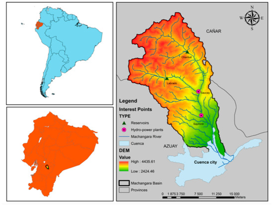
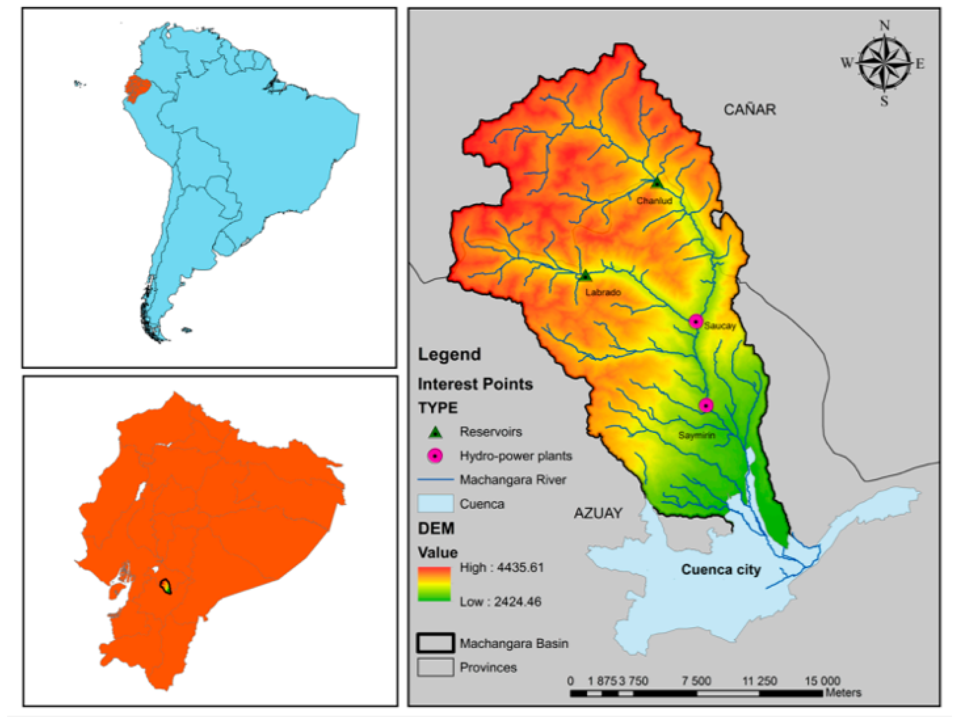
The Machángara River is located in an Andean basin between the provinces of Azuay and Cañar in southern Ecuador. It forms part of the Santiago hydrographic system and spans approximately 32,500 hectares [9]. Relative to Cuenca’s urban center, the river lies to the northeast, passing through the city’s industrial zone and the parishes of Checa, Chiquintad, Sinincay, and Ricaurte [10]. Figure 1 illustrates the geographical extent of the Machángara River Basin.

Figure 1. Machángara River Basin in southern Ecuador [7].

The region experiences two distinct seasons: a rainy season from mid-February to July, and a dry season that dominates the remainder of the year [10]. Average annual precipitation is approximately 3090 mm, with 2900 mm occurring during the rainy season and only 190 mm during the dry season [11]. However, seasonal patterns are not uniform, and deviations from expected rainfall can negatively impact agricultural productivity and water availability.

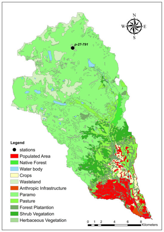
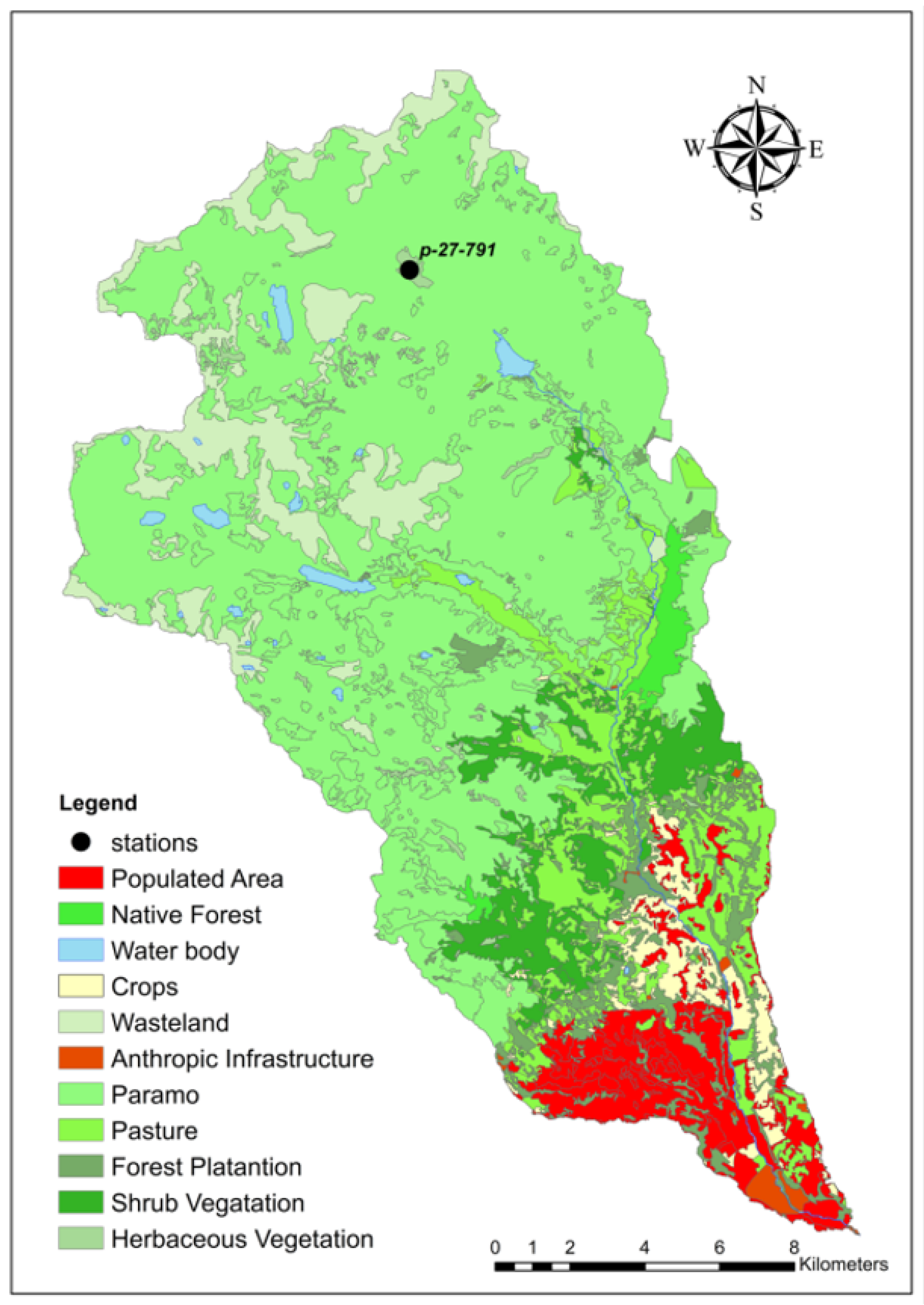
According to PROMAS [8], land use within the basin is distributed as follows: 6.4% urban area, 11.3% farmland, 0.5% infrastructure, 59.1% páramo (high-altitude grassland), 9.3% pasture, 1.2% native forest, 4.2% forest plantations, 6% shrub vegetation, 1% herbaceous vegetation, and 1% water bodies (Figure 2).

Figure 2. Distribution of land use in the Machángara River Basin.

2.1.2. Reservoirs, Electricity Production, and Other Uses of Water

Due to seasonal variability in precipitation, reservoirs play a critical role in stabilizing water supply. The basin contains two reservoirs (Chanlud and Labrado), two hydroelectric plants (Saucay and Saymirín), and one drinking water treatment facility, known as the Tixán Plant [4]. Commissioned in 1997, the Tixán Plant treats approximately 600 L per second and supplies potable water to around 140,000 residents in Cuenca and nearby parishes [9]. In addition to supporting domestic consumption and energy production, the system also provides irrigation water for approximately 1300 hectares, benefiting around 1900 users [9].

2.2. PSO Model for Optimization

Particle Swarm Optimization (PSO) was selected as the metaheuristic approach for optimizing the surface water allocation in the Machángara River Basin due to its algorithmic simplicity and suitability for complex, nonlinear problems. PSO does not require gradient information and relies solely on evaluating the objective function, making it ideal for black-box problems where model structure or derivatives are inaccessible [6,12].

In water resource systems governed by the WEF nexus, optimization often involves high-dimensional, nonlinear spaces. The calibration stage of this study, for example, required optimization 590,338 variables. PSO’s population-based search mechanism allows for efficient exploration of such large solution spaces. Compared to other algorithms like Genetic Algorithms (GA) or Differential Evolution (DE), PSO requires fewer hyperparameters and is less prone to premature convergence in high-dimensional contexts [13,14].

2.2.1. Overview of PSO

PSO is a heuristic algorithm that approximates global optima without guaranteeing their discovery. It is particularly effective for finding the maximum or minimum of a function defined in a multidimensional vector space [15]. Originally proposed by Kennedy and Eberhart [12], PSO was inspired by the collective behavior of bird flocks and fish schools. Each particle in the swarm represents a potential solution and adjusts its position based on its own experience and that of the swarm. At each iteration, a particle updates its position and velocity using the following equations:

Position update:

$X_i(t+1)=X_i\left(t\right)+V_i(t+1)$

Velocity update:

$V_i(t+1)=w·V_i\left(t\right)+c_1{r}_1·(pbes{t}_i-X_i\left(t\right))+c_2{r}_2·(gbest-X_i\left(t\right))$

• where

• w is the inertia weight,
• $c_1$ and $c_2$ are cognitive and social coefficients,
• $r_1$ and $r_2$ are random values between 0 and 1,
• $pbes{t}_i$ is the best position found by particle i,
• $gbest$ is the best position found by the entire swarm.

These parameters balance exploration and exploitation. A high $c_1$ with low $c_2$ may cause stagnation, while the reverse can lead to premature convergence.

2.2.2. Constraint Handling in PSO

Particles may violate constraints during the search process. To address this, strategies such as conflict counting and distance estimation are used [16]. Conflict counting penalizes constraint violations, while distance estimation measures how far a solution is from feasibility.

This study employs a repair function implemented via the Pymoo package [15], which adjusts particle values to better satisfy constraints. Although this improves compliance, it does not guarantee full constraint satisfaction.

To improve constraint satisfaction, a repair strategy was implemented using the Pymoo package. This strategy modifies infeasible solutions by projecting them into the feasible space. Mathematically, for a violated constraint $g_i\left(x\right)>0$, the following repair function applies:

$$x_{\mathrm{repaired}}=x-\lambda ·\nabla g_i\left(x\right)$$

(1)

where $\lambda$ is a scaling factor determined empirically, and $\nabla g_i\left(x\right)$ is the gradient approximation of the violated constraint. While this method improves feasibility, it does not guarantee convergence to a feasible global optimum.

2.2.3. Problem Modeling with Pymoo

The PSO model is implemented using the Pymoo package in Python 3.13.5 [15], which supports both single- and multi-objective optimization. Pymoo allows customization of hyperparameters, particle behavior, and constraint handling.

The problem is modeled as a matrix X, where each row represents a particle and each column corresponds to a decision variable. For example, in the calibration stage (1998–2001), the model includes 590,338 variables, resulting in a matrix of size $25\times 590,338$. Python dictionaries are used to track variable positions and construct constraints.

Each stage of the model—calibration, validation, and execution—has a different number of variables and constraints, based on the time period. Table 1 summarizes these values:

Table 1. Variable and constraint distribution across problem stages. This table outlines the number of decision variables, equality constraints, and inequality constraints assigned to each stage of the problem formulation.

Stage	Variables	Equality Constraints (=0)	Inequality Constraints ($\le 0$)
Calibration (1998–2001)	590,338	280,615	46,462
Validation (2002–2003)	293,552	139,532	23,070
Execution (2004–2005)	293,974	139,725	23,102

These preprocessing steps were foundational in ensuring that the PSO implementation could operate efficiently within the highly complex and constrained environment of the Machángara River Basin model.

2.3. Justification for Using PSO

The selection of Particle Swarm Optimization (PSO) as the heuristic framework for optimizing surface water allocation in the Machángara River Basin was grounded in both domain-specific advantages and algorithmic considerations.

First, PSO is particularly well suited to solving nonlinear, high-dimensional, and constraint-laden problems, such as those posed by the water–energy–food (WEF) nexus in hydrological systems. Unlike gradient-based methods, PSO operates without requiring derivative information, making it ideal for black-box models where the system dynamics are complex or partially observed.

Second, PSO’s population-based search mechanism provides robust global search capabilities, which are especially valuable when navigating thousands of interdependent variables, as demonstrated in this study’s calibration phase involving over 590,000 variables. Its simplicity of implementation and minimal hyperparameter requirements allow for scalable adaptation across different modeling stages (calibration, validation, and execution).

To contextualize PSO’s selection, the authors considered other widely used metaheuristic algorithms, such as Genetic Algorithms (GA) and Differential Evolution (DE). However, comparative studies [13,14] have shown that PSO can outperform these alternatives in maintaining diversity and escaping premature convergence in high-dimensional spaces. Specifically, algorithms like GA often demand more intensive parameter tuning and are prone to slower convergence in complex basin-scale resource allocation problems.

While PSO presents known challenges in constraint handling—particularly with equality constraints—the authors implemented repair strategies and adaptive hyperparameters to partially mitigate these limitations. The goal was to assess PSO’s feasibility as a standalone approach and establish a performance benchmark, prior to exploring hybrid variants in future work.

Thus, the contribution of this study lies in its application of PSO within a hydrological optimization context, testing its limits and documenting its interactions with real-world constraints and objectives. The results serve to inform both the limitations and potential of PSO in water resource management, setting the stage for method refinement and broader comparative assessments in subsequent phases.

Although PSO was selected for its simplicity and adaptability, a more robust comparative context is necessary. Metaheuristics such as Genetic Algorithms (GA), Differential Evolution (DE), and Ant Colony Optimization (ACO) have been widely applied in water resource optimization. For instance, GA offers strong global search capabilities but requires extensive parameter tuning. DE excels in continuous optimization but may struggle with constraint-heavy problems. ACO, while effective in discrete routing problems, is less suited for high-dimensional continuous domains like the Machángara Basin. PSO was chosen for its balance between exploration and exploitation, but future work should include formal benchmarking against these alternatives.

Preprocessing Techniques for PSO Implementation

Before applying the PSO algorithm to the water allocation model, a series of preprocessing techniques were implemented to prepare the data and structure the problem efficiently for optimization:

• Data Filtering and Temporal Segmentation: Hydrological data provided by PROMAS were segmented into three distinct periods—calibration (1998–2001), validation (2002–2003), and execution (2004–2005). This ensured temporal consistency and allowed each phase to be modeled independently within realistic boundaries.
• Variable Encoding and Structure Mapping: The river basin configuration, reservoir characteristics, and water demands were encoded using dictionaries and lists in Python. Each variable was indexed to facilitate rapid access and constraint formulation during the runtime.
• Dimensional Scaling: Variables such as daily water flow rates and reservoir levels were normalized based on statistical ranges derived from historical data. This prevented numerical instability during the swarm evaluations and improved the efficiency of parameter tuning.
• Matrix Construction for Particle Evaluation: A multidimensional matrix (X) was constructed, with each row representing a particle and each column corresponding to a problem variable. This $N\times D$ structure was essential for performance tracking and memory management during PSO iterations.
• Constraint Encoding: Equality and inequality constraints were algorithmically structured as vectorized functions in Python. This enabled fast evaluation and seamless integration with Pymoo’s repair function, which attempts to restore feasibility in violated constraint sets.
• Boundary Definition and Search Space Restriction: Each variable was assigned upper and lower bounds informed by operational ranges and ArcSWAT benchmarks. These bounds were strictly enforced to reduce unnecessary exploration and enhance convergence reliability.

2.4. Implementation Details

The PSO model was implemented in Python, using the Pymoo package [15], which offers flexibility for handling large-scale, constrained optimization problems. The implementation was customized to reflect the unique characteristics of the Machángara River Basin and to meet the specific requirements of the water–energy–food (WEF) nexus framework.

2.4.1. Variable Structure and Encoding

Each particle in the swarm represents a potential solution, encoded as a vector of decision variables. These variables correspond to water allocation decisions across different sectors and time steps. The structure is defined as follows:

• Matrix Representation: The swarm is represented as a matrix X, where each row corresponds to a particle and each column to a decision variable.
• Variable Indexing: Python dictionaries are used to map variable positions, enabling efficient access and constraint construction. This is particularly important given the high dimensionality—up to 590,338 variables in the calibration stage.
• Time-Dependent Modeling: Variables were indexed by time step, sector, and spatial unit, allowing dynamic modeling of water allocation throughout the study period.

2.4.2. PSO Configuration

The Particle Swarm Optimization (PSO) algorithm was configured using empirically tuned parameters to balance convergence speed and solution quality. The configuration is summarized in Table 2.

Table 2. PSO parameter settings. Summary of key parameters used in the PSO algorithm for water allocation modeling.

Parameter	Value	Description
Swarm Size	25 particles	Number of candidate solutions evaluated per iteration
Inertia Weight (w)	0.7	Balances global exploration and local exploitation
Cognitive Coefficient ($c_1$)	1.5	Influence of the particle’s personal best position
Social Coefficient ($c_2$)	1.5	Influence of the global best position across the swarm
Max Iterations	293,974	Termination criterion based on iteration count

These parameter values were selected based on preliminary testing and benchmarking against similar water resource optimization studies. The configuration aimed to ensure a robust search behavior, while maintaining computational efficiency.

2.4.3. Constraint Handling

Constraints were implemented using Pymoo’s built-in mechanisms, alongside custom repair functions:

• Equality Constraints: Represented as $g\left(x\right)=0$, these include mass balance equations and policy requirements.
• Inequality Constraints: Represented as $h\left(x\right)\le 0$, these encompass capacity limits, minimum flow thresholds, and sectoral priorities.
• Repair Function: A custom repair function modifies infeasible solutions by adjusting variable values to better satisfy constraints. While this improves feasibility, it does not guarantee full compliance.

2.4.4. Computational Considerations

Given the scale of the problem, the model was executed in a high-performance computing (HPC) environment with parallel processing capabilities. Efficient memory management and optimized data structures were essential to ensure scalability and prevent computational bottlenecks.

2.5. PSO Extension with Mixed Integer Linear Programming (MILP)

Building on prior work by Veintimilla-Reyes [4,7,17], the linear programming (LP) model was extended to a mixed integer linear programming (MILP) formulation. This enhancement enabled the selection of specific nodes within the water distribution network as candidate sites for constructing additional reservoirs with predefined capacities. The primary objective was to evaluate whether the performance of the water supply network (WSN) could be improved by strategically incorporating new reservoirs.

Although MILP components are integrated into the PSO framework, this implementation does not constitute a fully hybrid algorithm in the formal sense. The integration is limited to encoding binary decision variables within the PSO particle structure and evaluating them through an extended objective function. There is no dynamic interaction between the MILP solver and the PSO search process, nor is there a coordinated mechanism for constraint propagation or solution refinement across paradigms.

Accordingly, the model is more accurately described as a PSO with MILP-inspired encoding, rather than a true PSO–MILP hybrid. This distinction is important, as hybrid metaheuristics typically involve algorithmic coupling—such as alternating search phases, embedded solvers, or cooperative co-evolution strategies—that leverages the strengths of both methods [18,19].

The current encoding, while computationally tractable, lacks advanced integration features such as MILP-guided initialization, constraint-driven repair, or adaptive switching between heuristic and exact search modes. As a result, the PSO algorithm operates independently of MILP logic, and its ability to satisfy strict equality constraints remains limited, as evidenced by the high penalty costs and constraint violations documented in Section 3.

Future work should explore true hybridization strategies, including

• Embedding MILP solvers for local refinement of PSO-generated solutions.
• Designing cooperative frameworks, where MILP handles discrete decisions and PSO optimizes continuous variables.
• Implementing adaptive control mechanisms to switch between MILP and PSO based on convergence diagnostics or constraint satisfaction metrics.

2.5.1. Defining Candidate Reservoir Locations

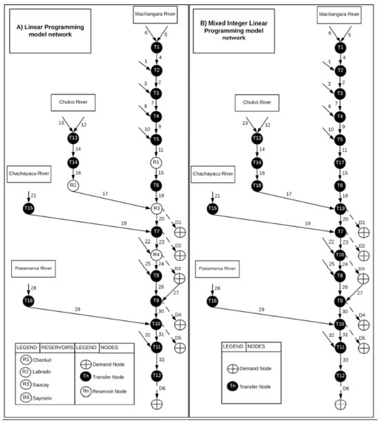
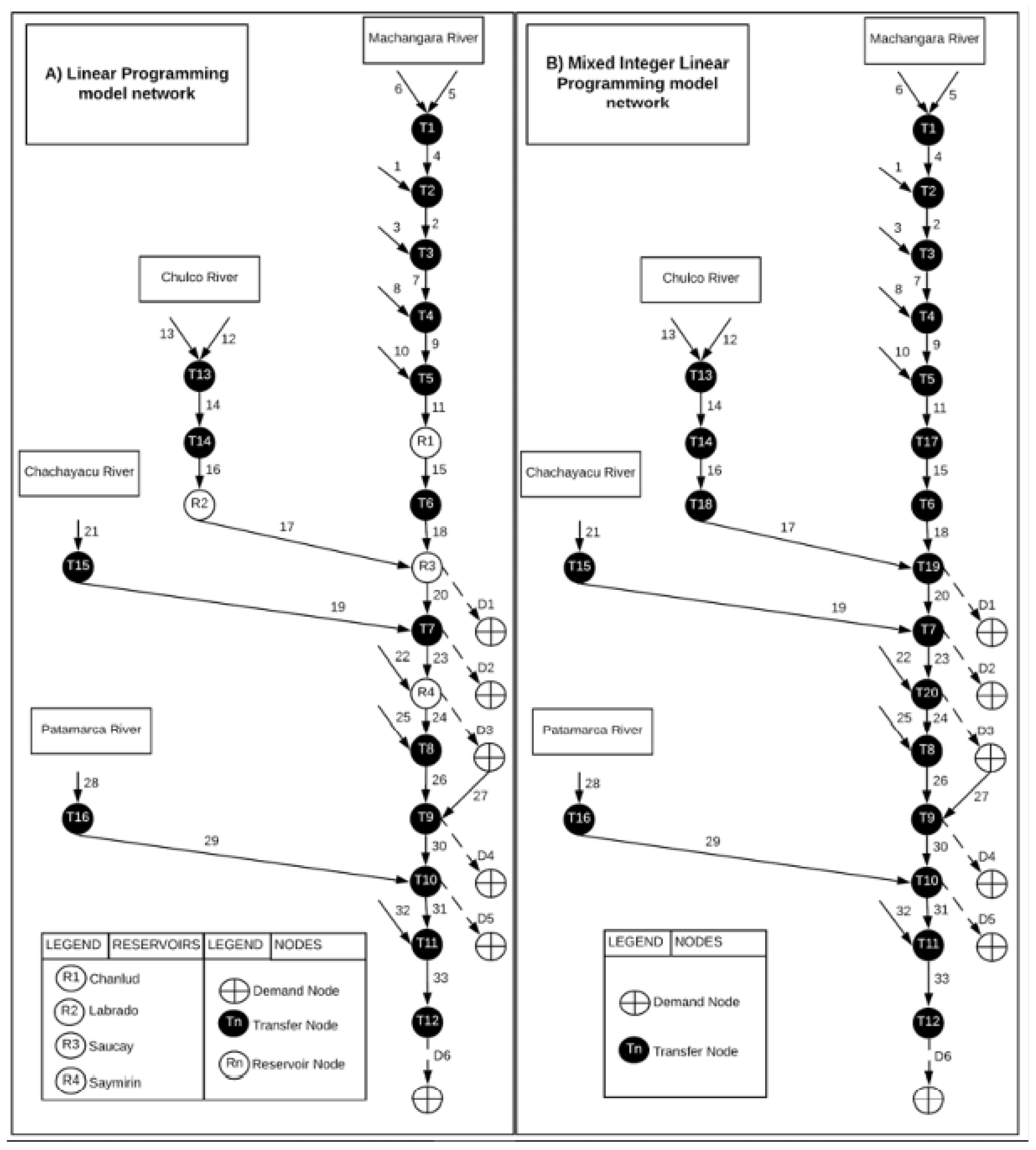
The network configuration for water allocation in the Machángara River basin comprises 4 reservoir nodes, 16 transfer nodes (which may function as reservoirs or facilitate water flow), and 6 demand nodes (representing water requirements). These nodes are interconnected by segments that enable water transfer throughout the network.

Figure 3 illustrates the network configurations used in the model. The left panel shows the base configuration, while the right panel depicts the extended version that includes candidate locations for new reservoirs. Both configurations share consistent parameters, decision variables, slack variables, and rainfall data.

Figure 3. Network configuration used in Veintimilla-Reyes (2022) [7] and adapted for PSO modeling. (A) Base configuration. (B) Extended configuration with all nodes considered as candidate reservoir locations.

2.5.2. Modeling the MILP Problem with PSO

In this formulation, transfer nodes are treated as “candidate reservoirs”—potential sites for constructing reservoirs with predefined capacities. The model aims to identify reservoir placements that minimize the total penalties associated with water distribution.

To achieve this, the water allocation model is extended to include penalties for unmet or exceeded demand, water shortages, reservoir overflows, violations of minimum flow requirements, flooding of river segments, and exceeding maximum flow capacities. Additionally, the model incorporates design, construction, and management costs for potential reservoirs. The objective function is expanded to include an estimated cost term ($B{C}_n$) for each candidate reservoir ($Y_n$), where $Y_n$ is a binary variable indicating whether location n is selected for reservoir construction [20].

The PSO algorithm was implemented using the Pymoo framework, with binary decision variables encoded within each particle and bounded between 0 and 1.

$$\begin{array}{cc}\hfill min& [\sum _n\sum (W_n·T_{n,n+1}^{t+})+\sum _n\sum _d\sum _t(P_n·S_{n,d}^{t-})+\sum _r\sum _t(U_r·S{H}_r^t)\hfill \\ \hfill & +\sum _r\sum _t(A_r·O{F}_r^{t+})+\sum _n\sum _t(B_n·Q_{n,n+1}^{t-1})+\sum _n\sum _d\sum _t(E_n+S_{n,d}^{t+})\hfill \\ \hfill & +\sum _n\sum _d\sum _t(F_n·MinX{D}_{n,d}^{t-1})+\sum _n\sum _d\sum _t(G_n·MaxX{D}_{n,d}^{t+})+\sum _n(B{C}_n·Y_n)]\hfill \end{array}$$

(2)

As in previous studies [4,7,17], two key characteristics are considered for candidate reservoirs:

• Storage capacity
• Minimum volume required to ensure sustainable operation

To incorporate these characteristics, the model adjusts reservoir capacity constraints and includes a restriction specifying the minimum number of reservoirs required. However, enforcing this constraint through PSO is challenging, due to the difficulty of satisfying strict equality constraints—even with repair mechanisms. Therefore, the PSO algorithm was configured to return the optimal number of reservoirs corresponding to the best objective function value found during the search.

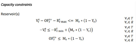
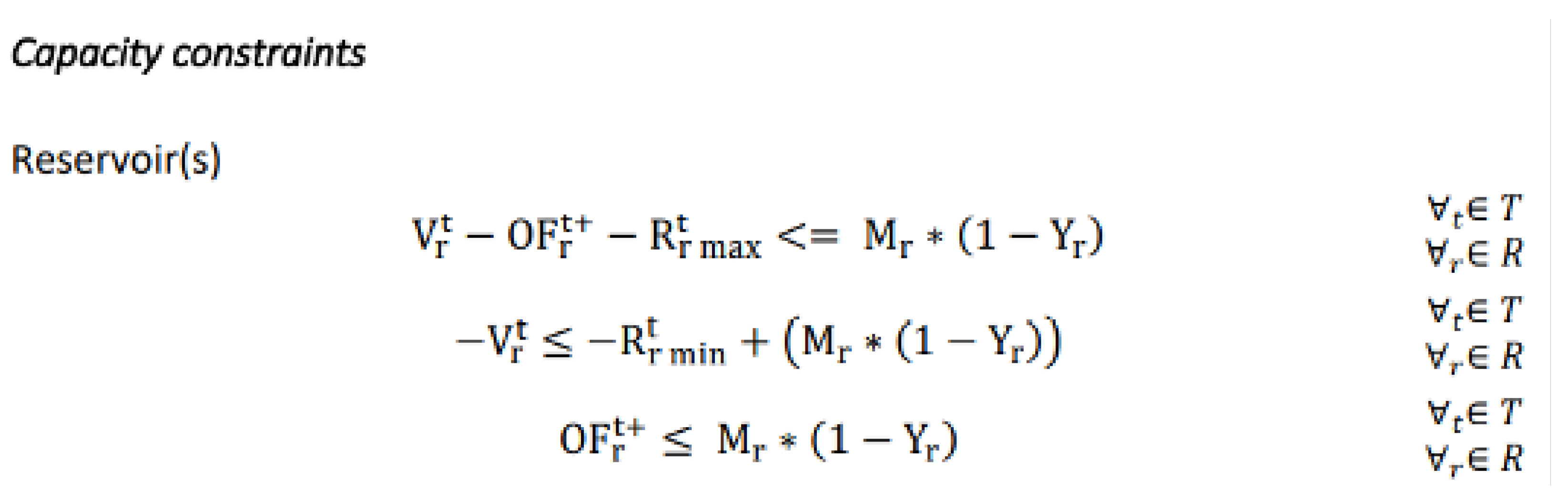
The parameter M (Figure 4) is defined as a sufficiently large constant to ensure that the equations hold under all feasible conditions. In this study, M is instantiated as a randomly generated 128-bit number to support binary encoding and constraint enforcement.

Figure 4. New constraints for reservoir construction.

2.5.3. Water Input, Reservoir Characteristics, and Water Demand

To estimate water inflow at each node—based on reservoir characteristics and the demand across various usage types—the same time periods and datasets used in the standard water allocation model were applied. Table 3 presents the attributes of both candidate and existing reservoirs, including initial volume; maximum capacity; minimum required volume; and biannual costs for design, construction, and management. Data were sourced from Veintimilla-Reyes (2022) [7].

Table 3. Reservoir attributes and cost parameters. Characteristics of candidate and existing reservoirs in the Machángara River basin.

Node	Type	Initial Volume [hm3]	Max Capacity [hm3]	Min Capacity [hm3]	Cost (€/2 years)
1, 2, 3	Candidate	2.6	13	1.3	195,000
4–16	Candidate	2.6	13	2.0	195,000
17	R1	5.0	6.15	1.23	150,000
18	R2	15.0	16.3	3.26	215,000
19	R3	0.7	1.0	0.2	100,000
20	R4	0.7	1.0	0.2	100,000

3. Results

3.1. Calibration, Validation, and Application of the Model

To maintain consistency with the linear programming methodology, this section follows the same three-phase structure—calibration, validation, and execution—previously applied to the LP model. However, each phase presents distinct challenges when implemented using heuristic methods such as Particle Swarm Optimization (PSO) [21]. In PSO, a population of particles (candidate solutions) explores the search space to identify optimal outcomes. As the number of particles and constraints increases, the probability of finding a solution that satisfies all constraints decreases significantly.

Seven model parameters require calibration, as listed in Table 4. As noted in earlier studies, observation data on water availability and flow within the river system were unavailable. Therefore, the water flow at the nodes—estimated using the ArcSWAT hydrological model—was used as a reference.

Table 4. Default values assigned to model parameters. Parameters used in the model prior to calibration.

Parameter	Default Value
Loss ($\alpha$)	0.001
Loss in flooded water ($\Delta$)	0.01
Time delays ($\delta$)	$1\times {10}^{-5}$
Time delays in flooded water ($\mu$)	0.001
Minimum water to stay ($\beta$)	0.01
Maximum water to stay ($\gamma$)	0.1
Loss in reservoirs ($\theta$)	0.001

The calibration phase used data from 1998–2001, the validation phase covered 2002–2003, and the execution phase applied data from 2004–2005. During calibration and validation, water demands were set to zero, shifting the focus from optimization to simulation. For PSO implementation, the number of particles, iterations, and execution threads must be specified. The algorithm was executed on the following machine:

• Intel^® Core™ i7-7700HQ CPU @ 2.80GHz
• 32 GB RAM
• Operating System: Windows
• Programming Language: Python 3.13.5
• PSO Implementation Package: Pymoo [15]

A trial-and-error approach was used to determine the computational limits of the machine, resulting in the following configuration:

• Number of particles: 25
• Number of iterations: 30
• Number of threads: 16

The number of decision variables, constraints, and evaluated functions varied across phases due to differences in the time periods considered. Specifically, the number of variables and constraints was proportional to the number of time steps (days) within each phase.

An important consideration is that the Pymoo documentation notes limitations in handling equality constraints. These constraints are rigid and pose challenges for black-box optimization problems [15]. While Pymoo performs adequately for problems with relatively few variables and constraints, its effectiveness diminishes as problem size increases—particularly when constraints are numerous and interdependent.

Moreover, since PSO generates solutions randomly, there is no guarantee that particles will satisfy all constraints. As the number and correlation of constraints increase, the likelihood of generating feasible solutions decreases substantially.

To evaluate model performance, the Root Mean Square Deviation (RMSD) was used:

$$RMSD=\sqrt{{\displaystyle \frac{1}{n}}\sum _{i=1}^n{(P_i-O_i)}^2}$$

(3)

where $P_i$ is the predicted value, $O_i$ is the observed value, and n is the number of observations.

3.1.1. Calibration

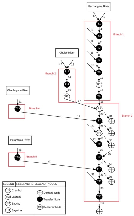
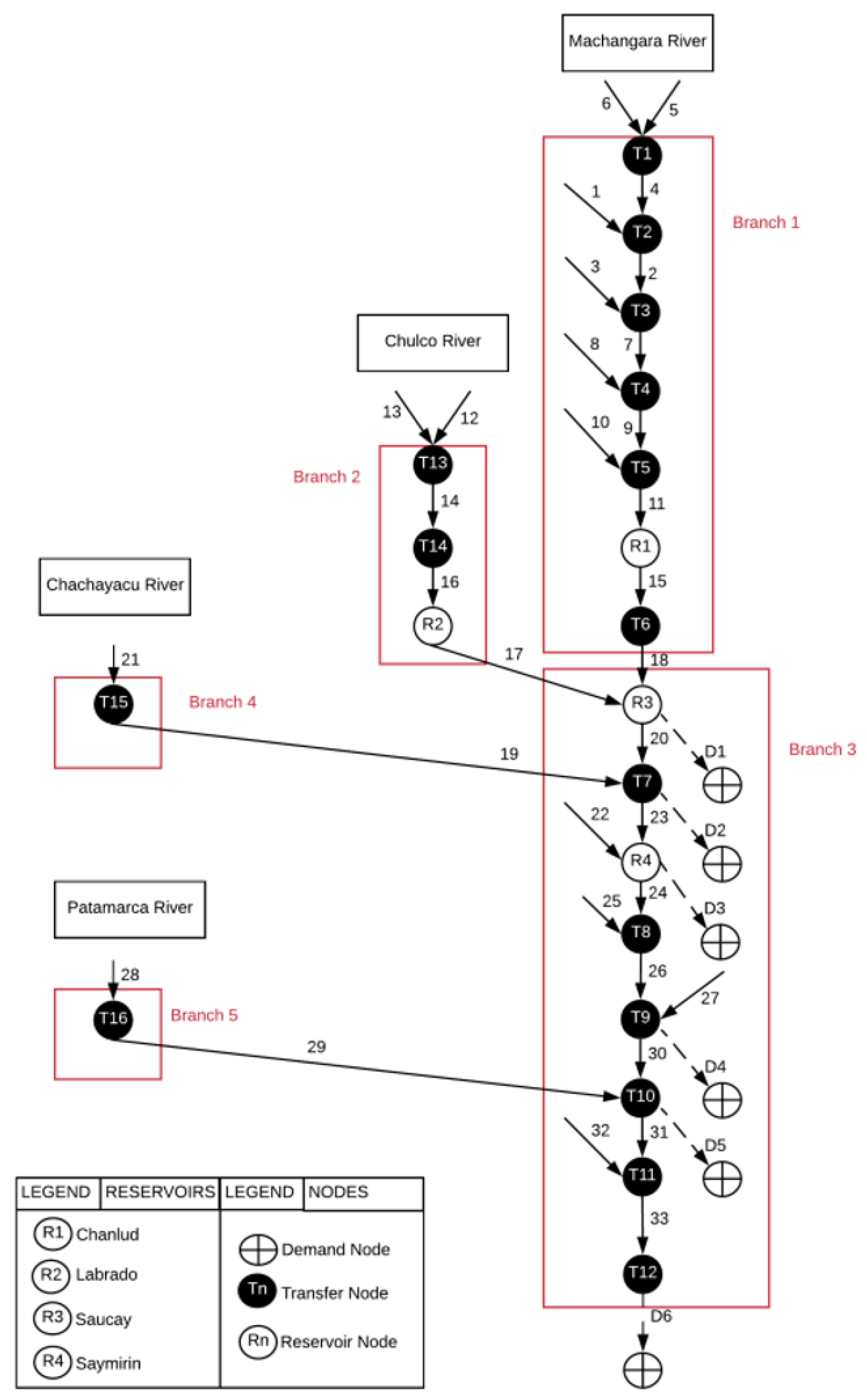
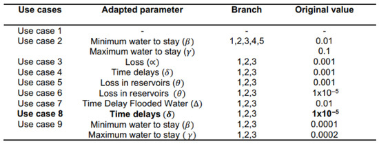
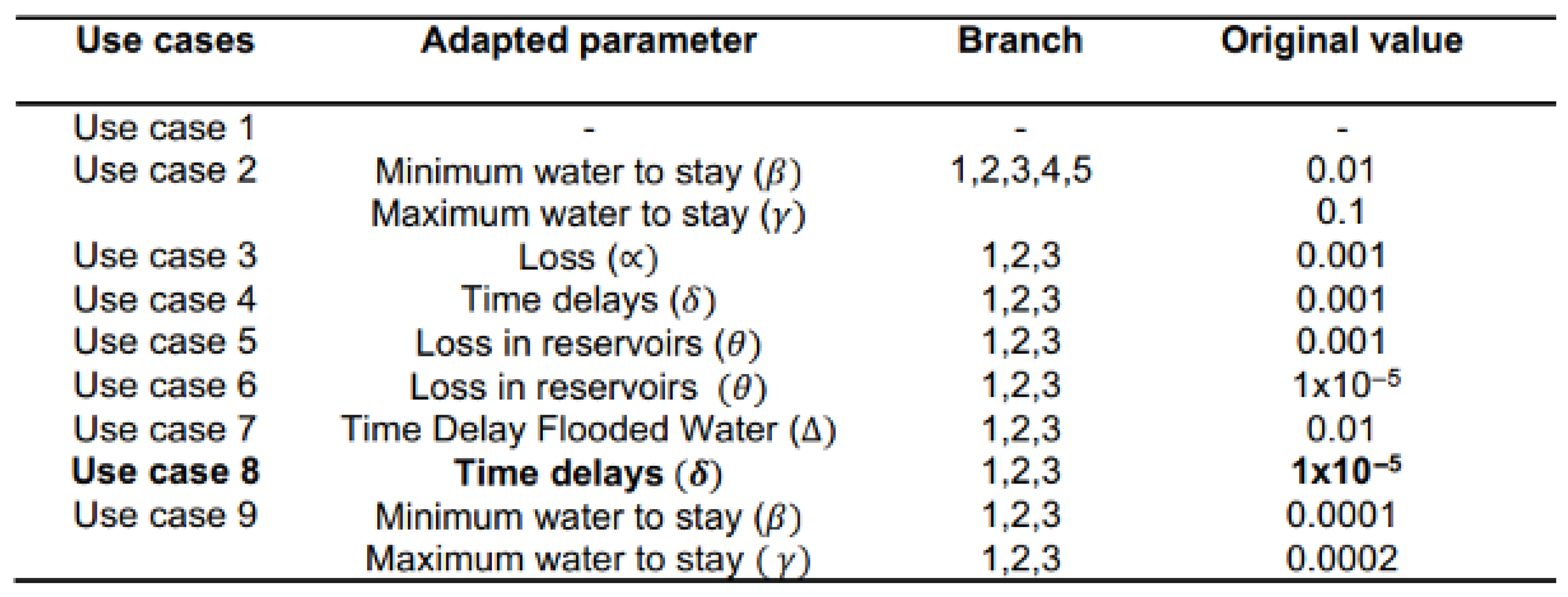
For the calibration phase, use cases from the previous study were considered, to ensure parameter calibration occurred within a consistent context. The Machángara River Basin network was divided into five branches based on segment connectivity, as illustrated in Figure 4. An iterative trial-and-error procedure was employed to adjust parameters according to the use case shown in Figure 5, aiming to minimize the discrepancy between PSO performance and reference values generated by ArcSWAT.

Figure 5. Branches of the Machángara River basin used for calibration.

Model performance was evaluated using the root mean square deviation (RMSD), defined in Equation (3), where $P_i$ represents the value calculated by the PSO model and $O_i$ denotes the corresponding value from ArcSWAT. RMSD quantifies the deviation of PSO-generated outputs (water values at each node) from those produced by the reference model.

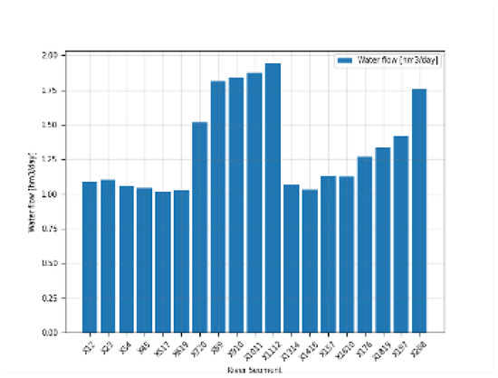
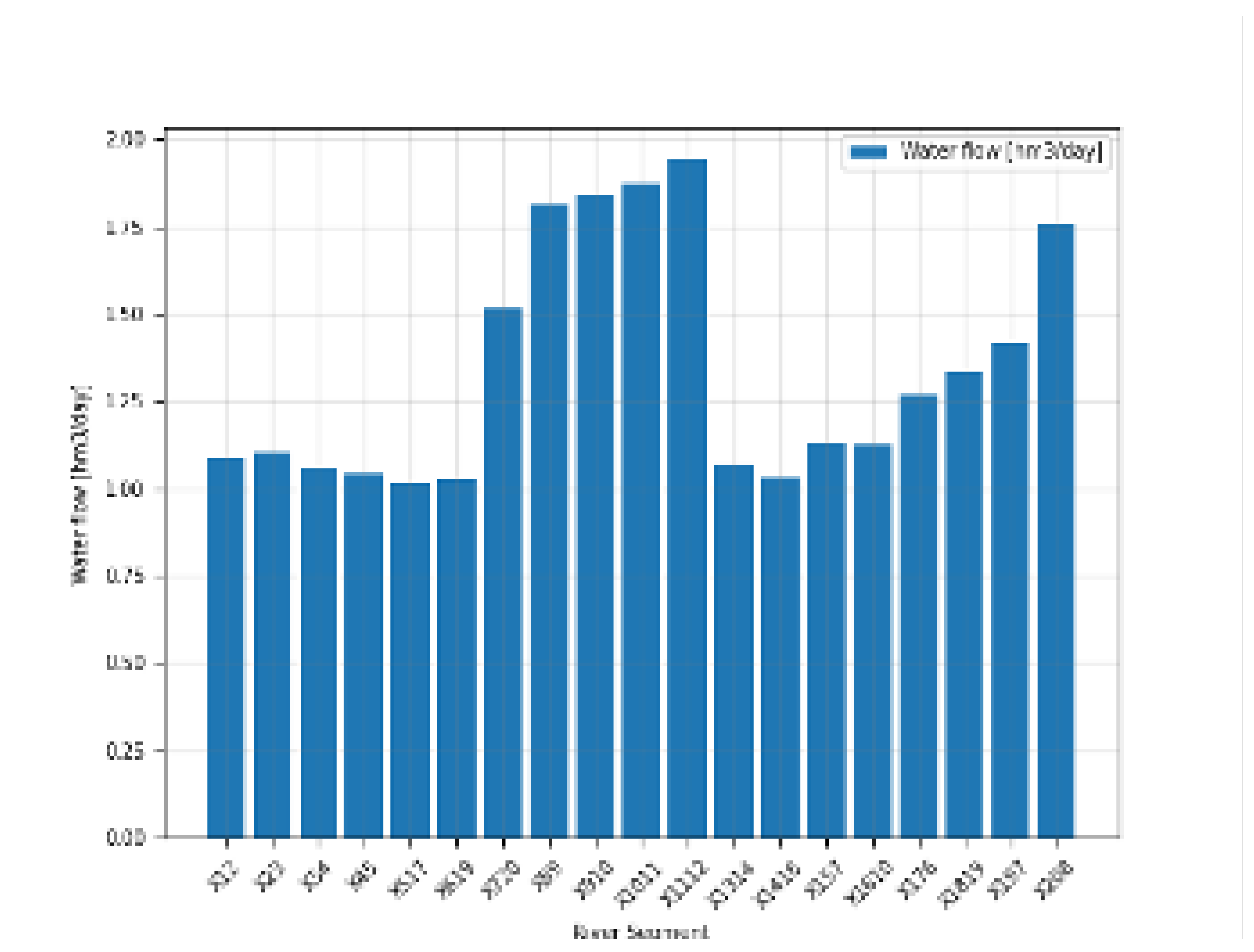
During the trial-and-error procedure, it was observed that the parameter adjustments did not significantly improve the simulation performance. Therefore, the model proceeded with default values, as shown in Figure 6. Figure 7 presents the RMSD for each river segment compared to the ArcSWAT values. The total RMSD was 25.4494 hm³. The execution time for 30 iterations was 2343.96 s (approximately 40 min), and the model successfully produced a solution.

Figure 6. Use cases from Lindfield (2009) [5], also applied for trial-and-error testing with PSO.

Figure 7. Root mean square deviation [hm³/day] between water flow simulated in ArcSWAT (reference) and the PSO model using default parameters for the 1998–2001 period.

3.1.2. Validation

For the validation phase, the model was executed using PSO without incorporating water demand values. The results were compared with ArcSWAT-generated time series for the 2003–2004 period (Figure 8). Parameters remained at their default values, as calibration adjustments did not yield significant improvements.

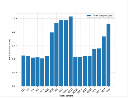
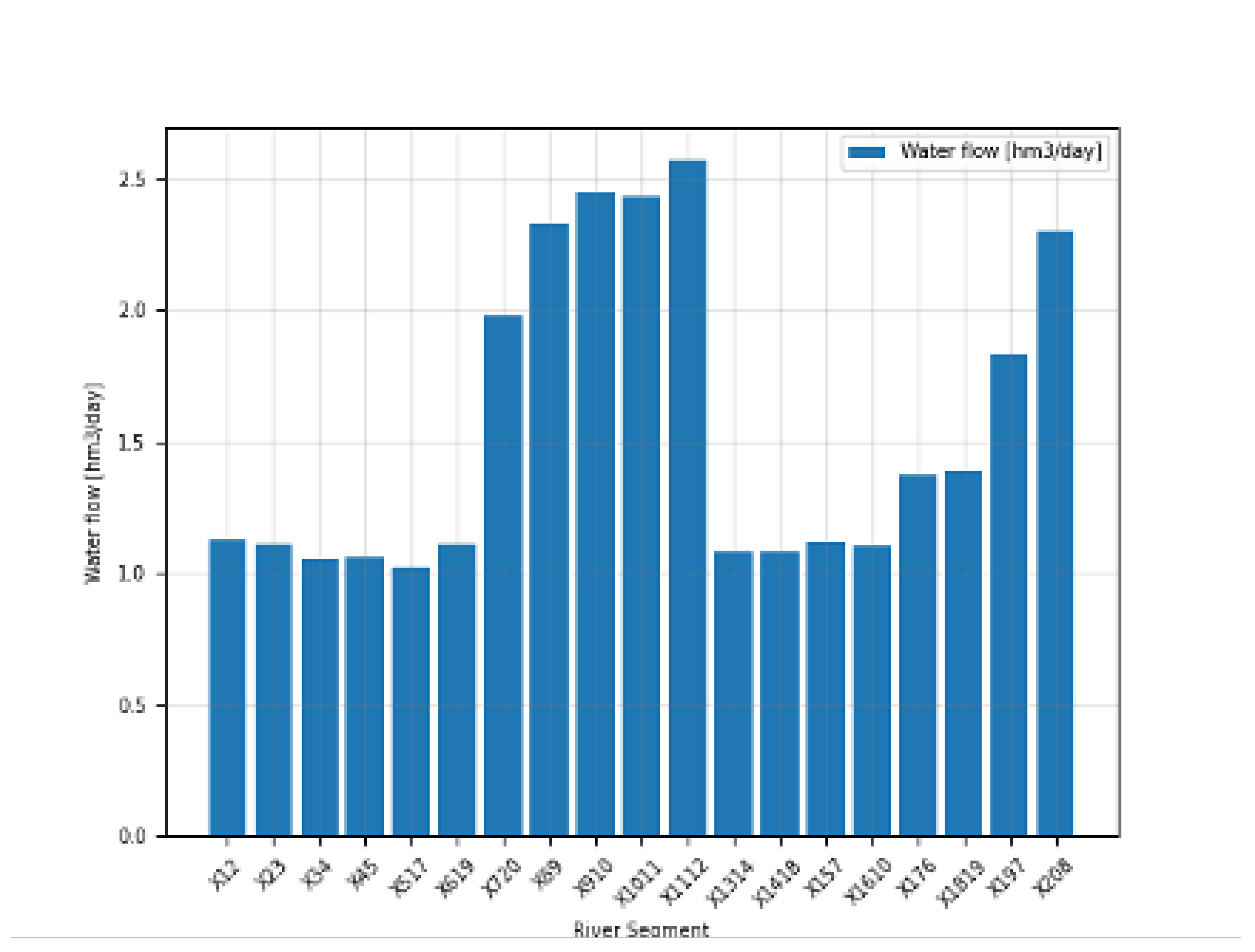
Figure 8. Root mean square deviation [hm³/day] between water flow simulated in ArcSWAT (reference) and the PSO model using default parameters for the 2003–2004 period.

The purpose of validation is to assess whether the selected parameter values remain appropriate under different conditions. In this run, the total RMSD was 29.5211 hm³, slightly higher than in the calibration phase. Parameter modifications did not noticeably affect the RMSD values. The execution time for 30 iterations was 1595.71 s (approximately 27 min), and the model successfully generated a solution.

3.1.3. Execution

The calibrated PSO model was applied to the 2004–2005 period, to optimally allocate the available water to demand nodes based on daily water requirements (Table 5). The allocation considered unit penalties for unmet or exceeded demands, as well as penalties associated with river segments, reservoirs, and demand nodes. The execution time for 30 iterations was 1067.01 s (approximately 18 min).

Table 5. Daily water requirements by demand nodes. Volume of water required per day by each demand node [7].

Node	Use	Value (hm3/day)
D1	Saucay Central	0.6208
D2	Machángara Irrigation System	0.0432
D3	Saymirín Central	0.6912
D4	Tixán Drinking Water System	0.12096
D5	Ricaurte Irrigation System	0.02592
D6	Ecosystem Functioning	0.01728

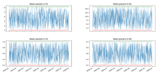
Figure 9 illustrates the total volume of water stored in each of the four reservoirs during the 2004–2005 period. Maximum values correspond to reservoir capacities listed in Table 6. The best result obtained by PSO satisfied some, but not all, of the minimum and maximum storage constraints. Additionally, the results did not align with seasonal rainfall patterns typical of the Machángara River Basin.

Figure 9. Volume of water stored in each reservoir in the Machángara River Basin during the 2004–2005 period.

Table 6. Storage capacities of reservoirs in the Machángara River Basin. Maximum and minimum water storage capacities of individual reservoirs.

Node	Reservoir	Min Capacity (hm3)	Max Capacity (hm3)
17	R1	1.23	6.15
18	R2	3.26	16.3
19	R3	0.2	1.0
20	R4	0.2	1.0

Reservoir R1 (Node 17), located upstream of the main Machángara River, generally maintained water levels between its capacity limits, but failed to exhibit stable flow patterns. Reservoir R2 (Node 18) is situated upstream in the Chulco sub-basin. Reservoirs R3 (Node 19) and R4 (Node 20) are located downstream and receive water from tributaries and regulated upstream inflows.

For R3 and R4, the seasonal rainfall patterns were less expected. Notably, the water volumes remained relatively similar across the system. Although the algorithm satisfied most constraints related to reservoir volumes, it failed to capture the seasonal variability and upstream influences.

3.1.4. Penalties

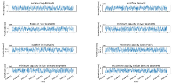
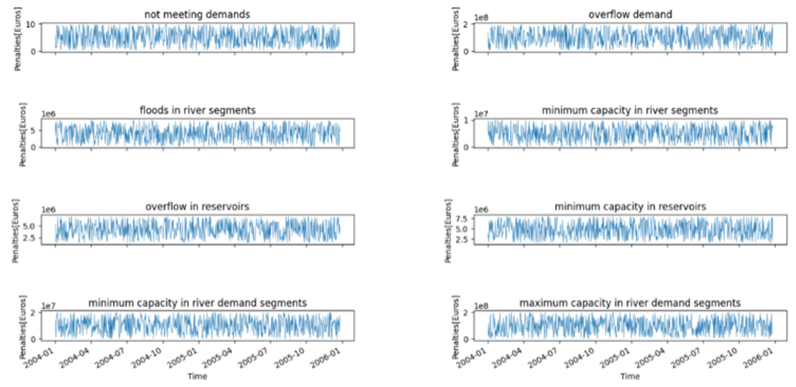
A penalty represents the cost incurred when water demand is unmet or when system constraints are violated, calculated per ${\mathrm{hm}}^3$. Based on the results in Table 7 and Figure 10, it is evident that the PSO model failed to achieve satisfactory optimization of water distribution across the Machángara River Basin. With a total penalty nearing EUR 164.95 billion, the model did not fulfill the objective of minimizing penalties while adhering to imposed constraints.

Table 7. Deviations from target water volumes and corresponding penalties. Differences (${\mathrm{hm}}^3$) between desired and optimized water volumes across demand nodes or time periods, with penalties expressed in euros.

Cause of Penalty	Volume [hm3]	Value [€]
(A) Unmet water demand	3696.02	3696.02
(B) Flooding claims	3656.93	73,138,624,526.29
(C) Flooding in river sections	725.61	2,902,452,589.12
(D) Violation of minimum river section capacity	717.12	3,585,641,307.33
(E) Flooding in reservoirs	434.52	3,041,687,022.49
(F) Violation of minimum reservoir capacity	437.34	3,498,729,001.97
(G) Violation of minimum demand segment capacity	3721.47	7,442,948,422.93
(H) Flooding in demand segments	3567.04	71,340,813,841.23
Total	16,956.08	164,950,900,407.42

Figure 10. Penalties generated by the model for each constraint during the 2004–2005 period.

Similarly to the case of the reservoir volumes, the PSO solution complied with certain restrictions but violated others. Moreover, the output failed to reflect seasonal rainfall patterns within the basin.

Summary of Key Findings

• Extreme penalty costs: The PSO model resulted in a total penalty of approximately EUR 165 billion, indicating major failures in satisfying water allocation constraints.
• Main contributors to penalty accumulation:

  –

  Overflow in demand segments generated the highest penalty: over EUR 71 billion.

  –

  Flooding claims and flooding in river sections together exceeded EUR 76 billion.

  –

  Violations of reservoir capacity constraints added more than EUR 6.5 billion.

• Unmet water demand:

  –

  Approximately 3696 ${\mathrm{hm}}^3$ of demand went unsatisfied.

  –

  Although relatively small in volume, these unmet demands still contributed to penalties and reflect PSO’s limitations in constraint handling.

• Mismatch with seasonal behavior:

  –

  Reservoir volumes failed to reflect realistic hydrological patterns, suggesting poor adaptability of PSO under time-dependent dynamics.

• Constraint violation issues:

  –

  PSO struggled with equality constraints, even when repair functions were applied, leading to frequent violations across multiple stages.

• Comparison with LP/MILP:

  –

  Linear and MILP models performed significantly better in constraint compliance and penalty minimization.

  –

  PSO’s attempt to construct additional reservoirs paradoxically increased the total penalty, a counterintuitive and unresolved outcome.

3.1.5. Convergence Analysis

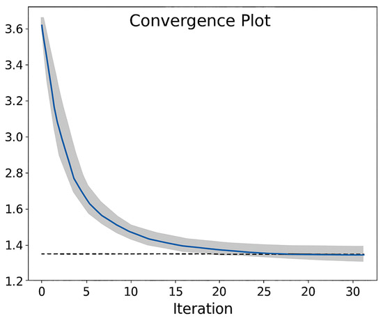
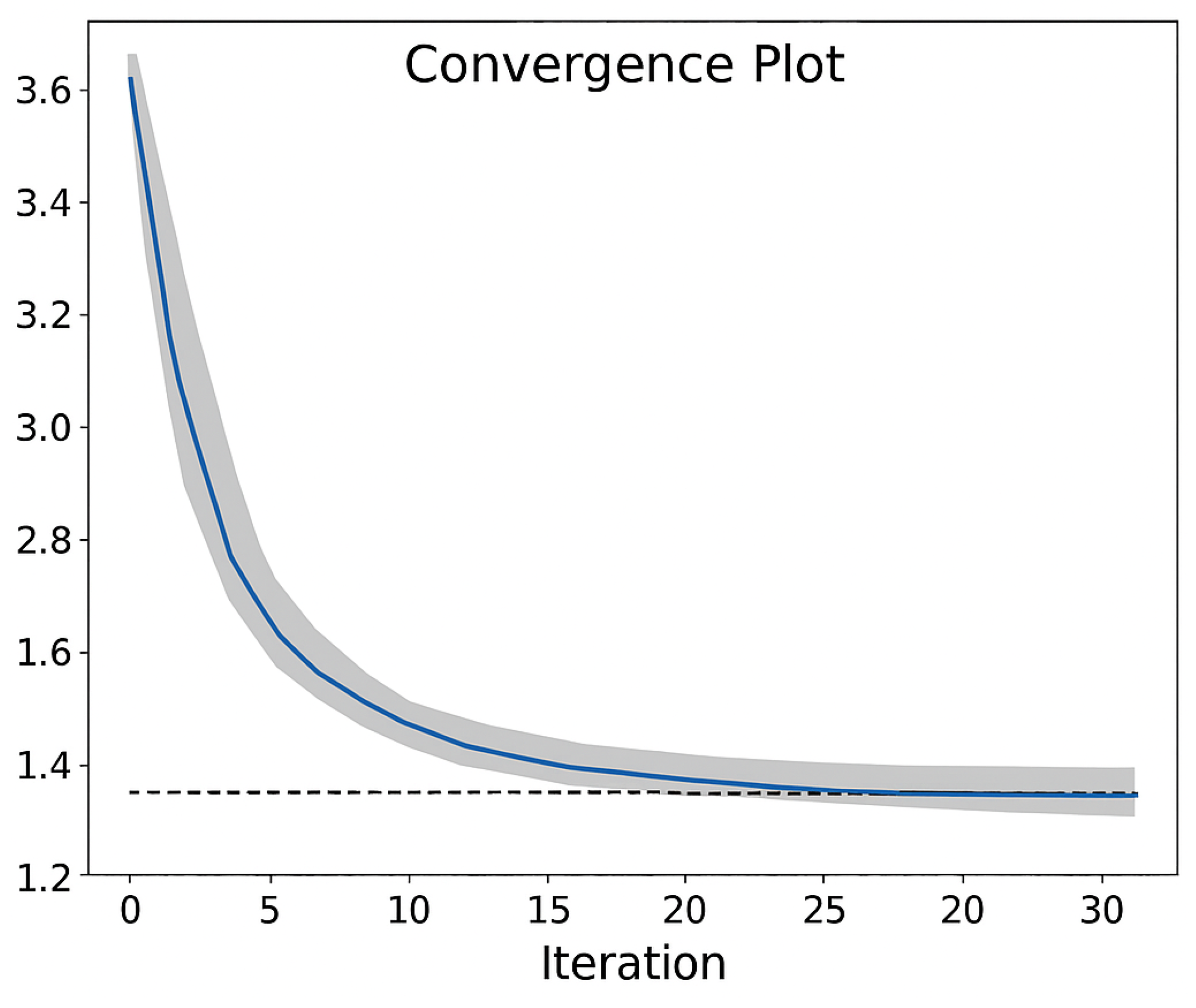
The convergence plot (Figure 11) reveals a typical optimization trajectory for Particle Swarm Optimization (PSO). During the initial phase (iterations 1–10), the algorithm exhibited rapid improvement in the best objective function value, indicating effective exploration of the search space. This behavior was driven by high swarm diversity and broad positional updates, allowing particles to escape local optima and discover promising regions.

Figure 11. Convergence plot showing the optimization trajectory of the PSO algorithm over 30 iterations.

After iteration 10, the curve flattens, suggesting premature convergence. This stagnation phase reflects reduced exploratory behavior, often caused by particles clustering around dominant solutions. The standard deviation of particle fitness values decreased from 0.12 to 0.03 over 30 iterations, quantitatively supporting this observation. A lower standard deviation implies that particles are evaluating similar solutions, limiting the algorithm’s ability to explore new regions.

This phenomenon—known as premature convergence—can hinder an algorithm’s ability to find global optima, especially in complex or multimodal landscapes. To mitigate this, future implementations may benefit from hybrid strategies, adaptive inertia weights, or diversity-preserving mechanisms such as re-randomization or mutation operators.

4. Discussion

4.1. Definition of Statistical Indicators for Model Comparison

A statistical indicator is a numerical value derived from a process that scientifically quantifies the characteristics of a sample [22]. These indicators may include the mean, median, and mode, among others, and are used to describe and analyze sample properties. When selecting an appropriate statistical indicator, factors such as data availability, resources required for quantification, study objectives, and other relevant considerations must be taken into account [23].

The objective of defining statistical indicators in this context was to enable a meaningful comparison between two methods for solving the water distribution optimization problem in the Machángara River Basin. The first method, discussed in [20], employed an exact mathematical approach known as Linear Programming (LP), while the second utilized a heuristic model referred to as Particle Swarm Optimization (PSO). Based on the available data from both methods, the following indicators were selected for comparison:

• Average and RMSD of constraint violations at each stage (calibration, validation, and execution).
• Total RMSD in each stage for the volume of water in river segments, compared to the values simulated by ArcSWAT.
• Average volume of unmet demand and corresponding penalty value in euros.

4.2. Comparison of PSO with Exact Mathematical Models (LP and MILP)

4.2.1. Comparison with LP

The first indicator used to compare the PSO and LP methods was the average number of constraint violations at each modeling stage. Unlike linear programming, which guarantees strict compliance with all constraints, the PSO algorithm exhibited difficulty in satisfying them consistently. This limitation was primarily attributed to the Pymoo package employed in this study, as most of its algorithms do not efficiently handle equality constraints. The rigidity of these constraints poses a particular challenge in black-box optimization problems [15].

Within the Pymoo framework, each constraint is formulated to evaluate to zero. Therefore, in an ideal scenario, both the average and root mean square deviation (RMSD) of constraint violations should also be zero. Table 8, Table 9 and Table 10 present the average and RMSD values for constraint violations during the calibration, validation, and execution stages, respectively.

Table 8. Average and RMSD of constraint violations during calibration. This table displays the mean and root mean square deviation (RMSD) values for each constraint used in model calibration. A value of zero indicates perfect compliance, meaning no constraint was violated.

Constraints	Average [hm3]	RMSD [hm3]
Related to water losses	0.6959	2.7893
Related to demand nodes	5.4570	24.1480
Related to losses and delays in demand nodes	0.2434	0.0829
Related to the minimum and maximum capacities
of a reservoir, as well as the loss of water in them	4.0308	24.3690
Related to flow capabilities	1472.31	7,191,836.09
Related to water flow delays	0.6272	0.3027
Related the maximum continuity of water	0.00	0.00
Related the minimum continuity of water	3.2254	7.5282
Related to water flow balance	3.4434	10.6633

Table 9. Average and RMSD of constraint violations during validation. This table presents the mean and root mean square deviation (RMSD) values for each constraint evaluated in the model validation phase. A zero value indicates complete compliance with the corresponding constraint.

Constraints	Average [hm3]	RMSD [hm3]
Related to water losses	0.7292	2.9718
Related to demand nodes	7.3565	65.3583
Related to losses and delays in demand nodes	0.1856	0.0514
Related to the minimum and maximum capacities
of a reservoir, as well as the loss of water in them	4.1350	25.9639
Related to flow capabilities	1473.4771	7,201,984.0736
Related to water flow delays	0.6226	0.2987
Related to the maximum continuity of water	0.00	0.00
Related to the minimum continuity of water	3.2288	7.5350
Related to water flow balance	3.4912	11.4564

Table 10. Average and RMSD of constraint violations during execution phase. This table presents the mean and root mean square deviation (RMSD) values for all constraints monitored during the model’s execution stage. A value of zero signifies full compliance with the defined constraints.

Constraints	Average [hm3]	RMSD [hm3]
Related to water losses	0.7090	2.8252
Related to demand nodes	5.4424	23.9631
Related to losses and delays in demand nodes	0.2417	0.0819
Related to the minimum and maximum capacities
of a reservoir, as well as the loss of water in them	3.9599	23.6774
Related to flow capabilities	1473.4720	7,201,962.6121
Related to water flow delays	0.6318	0.3054
Related to the maximum continuity of water	0.00	0.00
Related to the minimum continuity of water	3.2033	7.4270
Related to water flow balance	5.0226	40.2664

Across all three stages, the constraints related to maximum continuity of water were consistently satisfied. In contrast, the constraints associated with flow capacity exhibited the highest violation rates, followed by those concerning minimum and maximum reservoir capacities. These breaches indicate that reservoir water levels (as illustrated in Figure 9) occasionally exceeded or fell below the allowable limits.

Potential improvements could be achieved through a greater number of iterations, the integration of a hybrid PSO algorithm, or the adoption of alternative heuristic approaches. Nevertheless, in this case, it is evident that linear programming demonstrated a superior performance in terms of constraint compliance compared to PSO.

The second indicator used to compare the Linear Programming (LP) and Particle Swarm Optimization (PSO) methods was the total root mean square deviation (RMSD) at each stage. This metric reflects differences in the volume of water within river segments relative to the reference values simulated by ArcSWAT. Table 11 presents the RMSD values reported in [20] for the LP model, alongside those generated by the PSO model in this study.

Table 11. RMSD comparison across stages and optimization methods. This table presents the root mean square deviation (RMSD) values calculated for each stage of the modeling process, differentiated by the optimization method applied.

Stage	LP	PSO
Calibration	48.34	25.44
Validation	45.77	29.52

Table 11 shows that although PSO did not satisfy all constraints, it achieved a superior performance in terms of water volume within river segments. This improvement came from the use of upper and lower bounds derived from the maximum and minimum values simulated by ArcSWAT, which guided the particle exploration within a physically meaningful search space.

The difficulty in satisfying the remaining constraints stemmed from their dependence on combinations of multiple decision variables. While each variable may individually remain within its prescribed bounds, enforcing constraints based on their interactions introduces additional complexity. This suggests that increasing the number of iterations or employing a hybrid algorithm could enhance performance, enabling particles not only to respect individual bounds, but also to converge toward feasible solutions that satisfy all constraints.

As a final indicator, the average volume of unmet water demand and the corresponding penalty costs (in euros) were compared. Table 12 presents these penalty values. Although PSO yielded a lower RMSD, as shown in Table 11, its failure to satisfy all constraints resulted in significantly higher penalties for violating WEF-nexus requirements. Therefore, PSO may not be suitable for this optimization problem, unless a solution can be found within the multidimensional search space that simultaneously satisfies all constraints and minimizes penalties.

Table 12. Comparative penalty analysis: Linear Programming (LP) vs. Particle Swarm Optimization (PSO). This table compares the penalty costs incurred under the two optimization methods—LP and PSO—highlighting differences in constraint violations and solution efficiency.

Cause of the Penalty	PSO Vol. [hm3]	PSO Val. [€]	LP Vol. [hm3]	LP Val. [€]
(A) Sanction for not meeting demands	3696.02	3696.02	50.96	50.96
(B) Penalty for flooding claims	3656.93	73,138,624,526.29	0.00	0.00
(C) Penalty for flooding in river sections	725.61	2,902,452,589.12	0.00	0.00
(D) Sanction for not complying with the minimum capacity in the river sections	717.12	3,585,641,307.33	0.00	0.00
(E) Penalty for flooding in reservoirs	434.52	3,041,687,022.49	0.00	0.00
(F) Sanction for not complying with the minimum capacity in reservoirs	437.34	3,498,729,001.97	0.20	1.60
(G) Penalty for not meeting the minimum capacity in demand segments	3721.47	7,442,948,422.93	0.00	0.00
(H) Penalty for flooding in demand segments	3567.04	071,340,813,841.23	0.00	0.00
Total (A) + (B) + (C) + (D) + (E) + (F) + (G) + (H)	16,956.08	164,950,900,407.42	51.16	52.56

4.2.2. Comparison with MILP and PSO: Number of Optimal Reservoirs

The primary objective of the extended model, solved using Particle Swarm Optimization (PSO), was to determine which nodes—reservoirs or transfer points—should be converted into reservoirs based on predefined characteristics, including location, initial water level, minimum volume, and maximum capacity, in order to minimize total penalties.

The baseline results, which included the four existing reservoirs (Nodes 17, 18, 19, and 20), yielded a total penalty of EUR 164,950,900,407.42 during the execution stage. The extended model identified a configuration of 11 reservoirs that produced the lowest penalty with respect to the objective function. These reservoirs are listed in Table 13, with newly constructed reservoirs highlighted in bold.

Table 13. Reservoir construction selected by Particle Swarm Optimization (PSO) to minimize penalty costs. This table lists the reservoirs proposed for construction under the PSO method as the optimal solution to reduce system-wide penalty costs.

Reservoirs	Cost of Construction and Maintenance	Penalty [euros]
1, 2, 3, 4, 5, 6, 7, 8, 9, 10, 11, 12, 13, 14, 15, 16, 17, 18, 19, 20	2,145,000.00	168,196,407,013.80862

The model completed 30 iterations in a total execution time of 1239.46 s (approximately 20 min).

As shown in Table 14, no improvement was achieved by constructing additional reservoirs in the PSO-based resolution. This outcome aligns with the behavior reported in [5], which suggests that a single reservoir can sufficiently reduce the total penalty, indicating that the current basin configuration may not be optimal. In fact, using only one reservoir yielded a lower total penalty than the configuration with the four existing reservoirs when applying MILP. In the PSO scenario, adding up to 11 reservoirs did not reduce the penalty; instead, it resulted in a penalty increase. It is important to note that the maintenance cost data used are approximate and may differ from real-world values.

Table 14. Impact of single reservoir construction and maintenance on penalty costs. This table presents the construction and maintenance costs associated with implementing a single reservoir, alongside the penalties incurred for unmet water demands under this configuration.

Reservoirs	Cost of Construction and Maintenance	Penalty [euros]
1, 2, 3, 4, 5, 6, 7, 8, 9, 10, 11, 12, 13, 14, 15, 16, 17, 18, 19, 20	100,000.00	166,428,876,847.78842

To compare with the results from Veintimilla et al. (2019) [4] and Veintimilla (2022) [7], who identified the best outcome with a single reservoir in the system (R19), the model was adjusted to force the construction of reservoir 19—regardless of whether PSO selected that location as optimal. This was done to test if, under Pymoo’s implementation and PSO’s search nature, the equality constraints could be fully satisfied. However, Table 14 shows that building only reservoir 19 did not yield a lower penalty, nor did it improve the demand satisfaction compared to the scenario with the four existing reservoirs. Therefore, PSO is not an ideal method for determining the number of reservoirs to construct, as it failed to meet the equality constraints, which in turn led to increased penalties.

This study acknowledges that Linear Programming (LP) and Mixed-Integer Linear Programming (MILP) models outperform standard Particle Swarm Optimization (PSO) in satisfying operational constraints and minimizing penalties. These exact methods offer reliable feasibility and optimization precision, making them particularly suitable for regulatory and infrastructural planning.

However, the value of this research lies not in demonstrating methodological superiority, but in critically examining the performance boundaries of PSO within a constraint-rich hydrological scenario. By systematically documenting constraint violations, solution drift, and penalty accumulation, the study provides a grounded evaluation of standard PSO in real-world settings. These insights help clarify the limitations of PSO—and highlight opportunities where hybridization or adaptive strategies may bridge existing gaps.

Moreover, the investigation presents a detailed implementation framework using Python and Pymoo, enhancing accessibility for practitioners interested in heuristic modeling within similar basin systems. This clarity offers a foundation for future comparative studies, particularly those aiming to evaluate alternative metaheuristics under the Water–Energy–Food (WEF) nexus framework.

4.3. Benchmarking Framework for PSO-Based Water Allocation Optimization

To ensure the reliability, generalizability, and scientific rigor of the proposed PSO-based heuristic model for surface water allocation, a comprehensive benchmarking framework is essential. This framework enables systematic evaluation of algorithmic behavior across diverse problem landscapes and facilitates meaningful comparisons with alternative metaheuristics.

4.3.1. Benchmark Function Suite

A benchmarking suite should encompass a range of synthetic test functions that reflect the structural characteristics of water allocation problems, including nonlinearity, multimodality, and constraint complexity. Functions selected from the CEC 2005 and CEC 2017 repositories are particularly suitable, due to their standardized formulations and widespread adoption in metaheuristic evaluation [24,25].

• Unimodal functions (e.g., Sphere, Schwefel 2.22) assess convergence speed and exploitation capability.
• Multimodal functions (e.g., Rastrigin, Ackley, Griewank) evaluate exploration behavior and resilience to local optima.
• Hybrid composition functions simulate real-world complexity by combining multiple landscape features.

Each function should be evaluated in high-dimensional settings (e.g., 30 or 50 dimensions) to emulate the scale and intricacy of basin-level water resource systems.

4.3.2. Performance Metrics

To capture both optimization efficacy and behavioral dynamics, the following quantitative metrics are recommended [19,26]:

• Best-so-far fitness value: Tracks the minimum objective value achieved over time.
• Mean and standard deviation of final fitness: Reflects consistency and robustness across multiple runs (typically 30).
• Convergence speed: Defined as the number of iterations required to reach 90% of the best-known solution.
• Swarm diversity: Quantified using positional entropy and average pairwise Euclidean distance among particles, providing insight into the balance between exploration and exploitation.

These metrics collectively enable diagnosis of premature convergence, stagnation, and overfitting to local optima.

4.3.3. Comparative Metaheuristic Context

To justify the selection of PSO over other metaheuristics, it is imperative to establish a comparative baseline. Algorithms such as Genetic Algorithms (GA), Differential Evolution (DE), and Ant Colony Optimization (ACO) offer distinct advantages in terms of diversity retention, constraint handling, and discrete optimization, respectively [18,27].

A comparative study should be conducted under equivalent experimental conditions, including

• Identical benchmark functions and dimensionality
• Consistent stopping criteria and population sizes
• Parameter tuning via grid search or adaptive schemes

The statistical significance of performance differences should be assessed using non-parametric tests, such as the Wilcoxon signed-rank test for pairwise comparisons and the Friedman test for multi-algorithm ranking [28]. These tests ensure that observed differences are not attributable to stochastic variability alone.

4.3.4. Visualization and Diagnostic Tools

To enhance interpretability and support algorithmic refinement, the following visual diagnostics are recommended:

• Convergence plots: Illustrate the trajectory of the best fitness value across iterations, revealing phases of rapid improvement, stagnation, or oscillation.
• Diversity overlays: Superimpose swarm diversity metrics (e.g., positional entropy, pairwise distances) to identify transitions from exploration to exploitation.
• Annotated transitions: Highlight key behavioral shifts, such as clustering around local optima or re-exploration events triggered by repair or mutation strategies.

These visual tools offer intuitive insights into the algorithm’s dynamics and can inform the design of hybrid or adaptive variants [29].

5. Conclusions

To conclude, the PSO algorithm applied in this case study for water distribution in the Machángara River Basin proved suboptimal for reservoir allocation. A primary challenge lay in the inability of the particles—along with the Pymoo package used for implementation—to consistently identify solutions within a search space that satisfied all imposed constraints. Consequently, penalties increased due to unmet demands and violated restrictions.

Although constraint-handling strategies such as particle value repair can improve solution feasibility by guiding particles into the constrained space, these methods do not guarantee full compliance with all conditions. In the context of determining the optimal number of reservoirs, PSO failed to solve the problem effectively and often produced outcomes that were random. It neither satisfied the imposed constraints nor reduced the overall penalty; in fact, it tended to exacerbate it.

Another factor contributing to PSO’s inadequacy was the high dimensionality of the problem. The large number of decision variables imposes memory limitations, which restrict the number of particles and iterations that can be reasonably executed. This issue was compounded by a known drawback of PSO: the tendency for population diversity to diminish over time [30], making premature convergence common and requiring extensive iterations for particles to approach global or local optima.

In summary, standard PSO, as implemented via Pymoo in this study, was insufficient for solving the water allocation problem in the Machángara River Basin under strict system constraints. The algorithm struggled to satisfy the equality conditions and yielded suboptimal solutions, with elevated penalty costs.

Nonetheless, the scientific contributions of this study include

• Quantifying PSO’s limitations across calibration, validation, and execution phases.
• Evaluating constraint-handling strategies, such as repair functions, within high-dimensional search spaces.
• Establishing empirical benchmarks to inform the development of future hybrid or adaptive heuristic models.

While LP and MILP remain the preferred methodologies for this class of optimization problem, this research highlights the technical shortcomings of PSO and lays the groundwork for exploring more advanced heuristic techniques in environmental resource management.

Finally, it is worth noting that prior literature identified PSO as one of the most widely used and efficient algorithms for similar problems. However, those implementations typically involved hybrid variants that incorporated enhancements to improve constraint satisfaction. Future work should explore hybrid PSO algorithms with improved handling of equality constraints and enhanced convergence behavior in complex search spaces.

References

- Liu, P.; Zou, H.; Guo, S.; Zeng, Y.; Shen, Y.; Liu, D.; Zhang, J.; Xiong, L.; Tian, J. Optimisation of water-energy nexus based on its diagram in cascade reservoir system. J. Hydrol. 2018, 569, 347–358. [Google Scholar] [CrossRef] [Scilit]
- Yang, Y.; Luo, Q.; Ye, G. Optimization of water allocation system at the river basins. In Proceedings of the 2018 14th International Conference on Natural Computation, Fuzzy Systems and Knowledge Discovery (ICNC-FSKD), Huangshan, China, 28–30 July 2018; pp. 482–488. [Google Scholar] [CrossRef] [Scilit]
- Haro, D.; Paredes, J.; Solera, A.; Andreu, J. A Model for Solving the Optimal Water Allocation Problem in River Basins with Network Flow Programming When Introducing Non-Linearities. Water Resour. Manag. 2012, 26, 4059–4071. [Google Scholar] [CrossRef] [Scilit]
- Veintimilla-Reyes, J.; Meyer, A.D.; Cattrysse, D.; Tacuri, E.; Vanegas, P.; felipe Cisneros; Orshoven, J.V. MILP for Optimizing Water Allocation and Reservoir Location: A Case Study for the Machángara River Basin, Ecuador. Water 2019, 11, 1011. [Google Scholar] [CrossRef] [Scilit]
- Lindfield, G.; Penny, J. Numerical Methods Using MATLAB®; IEEE: New York, NY, USA, 2009. [Google Scholar]
- Labadie, J.W. Optimal Operation of Multireservoir Systems: State-of-the-Art Review. J. Water Resour. Plan. Manag. 2004, 130, 93–111. [Google Scholar] [CrossRef] [Scilit]
- Veintimilla-Reyes, J. Mathematical programming for the support of river water management: Water allocation and reservoir location. KULeuven 2022. [Google Scholar]
- PROMAS. Programa para el Manejo del Agua y el Suelo. 2019.
- ETAPA, E.P. ETAPA EP—ETAPA EP—Servicios de Telefonía, Televisión, Internet, Agua Potable, Alcantarillado de Cuenca—Ecuador > Principal > Agua Potable, n.d. 2022.
- Villavicencio Riera, V.E.; Chávez Ochoa, L.M. Estudio Arqueológico en las Cuencas Media y Bajas del río Machángara. Available online: https://repositorioslatinoamericanos.uchile.cl/handle/2250/1110239?show=full (accessed on 18 June 2025).
- Jerves-Cobo, R.; Everaert, G.; Iñiguez-Vela, X.; Córdova-Vela, G.; Díaz-Granda, C.; Cisneros, F.; Nopens, I.; Goethals, P.L.M. A methodology to model environmental preferences of EPT taxa in the Machangara River Basin (Ecuador). Water 2017, 9, 195. [Google Scholar] [CrossRef] [Scilit]
- Kennedy, J.; Eberhart, R. bls gov. In Particle Swarm Optimization; Technical report; 1995. [Google Scholar]
- Shi, Y.; Eberhart, R. Modified particle swarm optimizer. In Proceedings of the IEEE Conference on Evolutionary Computation, ICEC, Anchorage, AK, USA, 4–9 May 1998; IEEE: New York, NY, USA, 1998; pp. 69–73. [Google Scholar] [CrossRef] [Scilit]
- Clerc, M.; Kennedy, J. The particle swarm—Explosion, stability, and convergence in a multidimensional complex space. IEEE Trans. Evol. Comput. 2002, 6, 58–73. [Google Scholar] [CrossRef] [Scilit]
- Blank, J.; Deb, K. Pymoo: Multi-Objective Optimization in Python. IEEE Access 2020, 8, 89497–89509. [Google Scholar] [CrossRef] [Scilit]
- Lin, I.L.; Fraser, S. Particle swarm optimization for solving constraint satisfaction problems. 2002.
- Veintimilla-Reyes, J.; Meyer, A.D.; Cattrysse, D.; Orshoven, J.V. From Linear Programming Model to Mixed Integer Linear Programming Model for the Simultaneous Optimisation of Water Allocation and Reservoir Location in River Systems. Proceedings 2018, 2, 594. [Google Scholar] [CrossRef] [Scilit]
- Talbi, E.G. Metaheuristics: From Design to Implementation; John Wiley & Sons: Hoboken, NJ, USA, 2009; p. 593. [Google Scholar]
- Boussaïd, I.; Lepagnot, J.; Siarry, P. A survey on optimization metaheuristics. Inf. Sci. 2013, 237, 82–117. [Google Scholar] [CrossRef] [Scilit]
- Veintimilla-Reyes, J.; Meyer, A.D.; Cattrysse, D.; Orshoven, J.V. A linear programming approach to optimise the management of water in dammed river systems for meeting demands and preventing floods. Water Sci. Technol. Water Supply 2017, 18, 713–722. [Google Scholar] [CrossRef] [Scilit]
- Jayaram, M.A. How should I design PSO particles for large number of decision variables? 2024.
- Aguilar, A.S. GUIA PRACTICA “CONSTRUCCIÓN E INTERPRETACIÓN DE INDICADORES ESTADÍSTICOS” Preparado por: Mg. Aníbal Sánchez Aguilar. 2004.
- Indicadores. Indicadores. 2024.
- Li, X.; Omidvar, M.N.; Qin, K.; Tang, K.; Omidvar, M.N.; Yang, Z. Benchmark Functions for the CEC’2013 Special Session and Competition on Large-Scale Global Optimization; Technical report; 2013. [Google Scholar]
- Liang, J.; Runarsson, T.P.; Mezura-Montes, E. Problem Definitions and Evaluation Criteria for the CEC 2006 Special Session on Constrained Real-Parameter Optimization; Technical report; 2006. [Google Scholar]
- Eiben, A.E.; Smith, J.E. Introduction to Evolutionary Computing; Springer: Berlin/Heidelberg, Germany, 2003. [Google Scholar] [CrossRef] [Scilit]
- Das, S.; Suganthan, P.N. Differential evolution: A survey of the state-of-the-art. IEEE Trans. Evol. Comput. 2011, 15, 4–31. [Google Scholar] [CrossRef] [Scilit]
- Derrac, J.; García, S.; Molina, D.; Herrera, F. A practical tutorial on the use of nonparametric statistical tests as a methodology for comparing evolutionary and swarm intelligence algorithms. Swarm Evol. Comput. 2011, 1, 3–18. [Google Scholar] [CrossRef] [Scilit]
- Zhang, J.; Zhan, Z.h.; Lin, Y.; Chen, N.; Gong, Y.j.; Zhong, J.h.; Chung, H.S.; Li, Y.; Shi, Y.h. Evolutionary Computation Meets Machine Learning: A Survey. IEEE Comput. Intell. Mag. 2011, 6, 68–75. [Google Scholar] [CrossRef] [Scilit]
- Lai, V.; Huang, Y.F.; Koo, C.H.; Ahmed, A.N.; El-Shafie, A. A Review of Reservoir Operation Optimisations: From Traditional Models to Metaheuristic Algorithms. Arch. Comput. Methods Eng. 2022, 29, 3435–3457. [Google Scholar] [CrossRef] [Scilit] [PubMed]
Disclaimer/Publisher’s Note: The statements, opinions and data contained in all publications are solely those of the individual author(s) and contributor(s) and not of MDPI and/or the editor(s). MDPI and/or the editor(s) disclaim responsibility for any injury to people or property resulting from any ideas, methods, instructions or products referred to in the content. |
© 2025 by the authors. Licensee MDPI, Basel, Switzerland. This article is an open access article distributed under the terms and conditions of the Creative Commons Attribution (CC BY) license (https://creativecommons.org/licenses/by/4.0/).