Modeling Hydraulic Transient Process in Long-Distance Water Transfer Systems Using a MUSCL-Type FVM Approach

Abstract

To gain deeper insights into the influence of pipe parameters on water hammer properties and achieve the accurate simulation of the hydraulic transient process in pipeline systems, the Finite Volume Method (FVM) is adopted. The solution scheme, incorporating a second-order MUSCL-type reconstruction, is derived, and the numerical solution process is detailed. For enhanced accuracy, the unsteady friction term is included in the numerical solution of the governing water hammer equations. The method is validated through a comparison with experimental data and the verification of mesh and Courant number independence, confirming both its efficiency and accuracy. The calculation error of the peak water head is less than 5%. Finally, an engineering case is studied to investigate valve arrangement and operation. Optimization yields the optimal valve position and operating parameters. This analysis provides valuable reference for pipeline system design.

1. Introduction

Pipes are core components of critical hydraulic infrastructure, including long-distance water transmission networks, pumped-storage power stations, and municipal water distribution systems. Ensuring hydraulic safety is essential for maintaining their operational stability [1,2,3,4,5]. However, events such as pipe breakage or pump failure can induce water hammer, significantly increasing internal pressure and potentially causing severe damage to the pipeline system. Consequently, the accurate simulation of hydraulic transients is fundamental for effective system design and protection. Furthermore, optimizing design of the pipeline system represents a key strategy for reducing water hammer impacts.

Hydraulic transient analysis is the basis for predicting water hammer properties. In current research, several approaches have been applied to calculate the hydraulic transient process in pipeline systems. Among these methods, the Method of Characteristics (MOC) has the widest application due to its ease of application and high accuracy [6,7]. Using the MOC method, the water hammer equations are transformed into ordinary differential equations, and both the pressure and the mass flow rate in the system can be obtained. However, when the pipeline system is complicated, e.g., with numerous short pipes, interpolation is needed or the model must be simplified first in the calculation, which decreases the analysis accuracy. Moreover, although pressure peaks and cavity evolutions can be simulated, there is often an error between the simulated pressure wave phase/peak and experimentally obtained results [8]. Hence, as an alternative, the finite volume method (FVM) draws attention. In Zhao’s research [9], the FVM was applied to analyze flow characteristics in a pipeline system and both first-order and second-order Godunov-type solution schemes were derived; the MOC method was also used for comparison, and the results showed that the second-order FVM had higher accuracy. In Zhou’s research [10], the second-order FVM scheme was studied and the MINMOD limiter was applied, and the results showed its effectiveness in analyzing transient cavitation cases. The unsteady friction term was also considered and the second-order Godunov scheme was derived, with the results showing high accuracy [11]. Compared to the MOC method, the FVM is more flexible for solving engineering problems. The second-order FVM scheme is robust and effective when the Courant number is less than one. Once the unsteady friction term was considered, the solution accuracy can be further enhanced. The Zielke model and the Brunone model are most commonly used to determine unsteady friction [12]. The Zielke model involves convoluting all previous fluid accelerations to achieve high accuracy, but the calculation is time-consuming. The Brunone model is easier to use, but for the MOC method, the requirement of the interpolation decreases accuracy. Compared to analyses omitting the unsteady friction model, including it significantly enhances analysis accuracy. To reduce water hammer’s influence on pipeline systems, the optimization of pipe parameters and valve closure regulation has been studied [13,14]. The optimization of water hammer control devices in pipelines was considered [15]; a system model was established and the hydraulic transient process was simulated; and the Differential Evolution method was used to optimize the size, location, and number of air valves. In LI’s research [16], the optimization of water hammer protection device arrangement was discussed, and the transient positive and negative pressure heads were both decreased. To decrease water hammer’s influence, valve closure regulation was also discussed. Commonly, fast valve adjustment is needed during pipe system operation; however, rapid valve closure can dramatically increase pipe pressure, potentially damaging the system. Hence, valve closure regulation is important in pipe operation [17,18]. A two-stage valve closure strategy was studied by Xin et al., and a water hammer protection method was discussed [18]. Flow characteristics during valve operation were discussed, showing that pipe parameters significantly influence water hammer [19,20]. Commonly, a two-stage valve closure strategy is considered for pipe operation. Valve operation is essential for the safety of water conveyance pipelines and pumped-storage power stations. Hence, the design optimization of valve operation rules and valve placement becomes essential, requiring a particular discussion about optimization strategies.

In this research, a second-order MUSCL-type FVM solution scheme is proposed for hydraulic transient analysis. Firstly, the unsteady friction term is incorporated using the Brunone model, and the fundamental formulation of the second-order FVM scheme is derived from the governing water hammer equations. The solution accuracy is verified through a comparison between the simulation results and experimental data. Then, an engineering case is considered and both the position and operation rules of a valve are optimized. Approximate models for maximum and minimum water heads, represented by pipe parameters and valve operational parameters, are established using the radial basis function (RBF) method. Finally, optimization yields the optimal valve position and closure parameters. The influence of pipe parameters on water hammer characteristics is further investigated.

2. Governing Equations

2.1. Basic Equations for Flow Analysis

The governing equations for pipe flow consist of the continuity and momentum equations, expressed as Equations (1) and (2):

$$H_t+V{H}_x+{\displaystyle \frac{a^2}{g}}{V}_x=0$$

(1)

$$V_t+g{H}_x+V{V}_x+J_q+J_u=0$$

(2)

where H is the water head, V is the flow velocity, a is the acoustic wave speed, g is the gravitational acceleration, t is the flow time and x means the axial coordinate along the pipe. J_u is the unsteady friction term and J_q is the quasi-steady friction term, which is defined as (3)

$$J_q={\displaystyle \frac{f_{q}V\left|V\right|}{2D}}$$

(3)

where D is the pipe diameter and f_q is the quasi-steady friction coefficient, which is determined by using the Hagen Poiseuille law or the Colebrook–White formula.

Several models are available for characterizing the unsteady friction term. Among them, the Brunone model is widely applied due to its implementation ease and high accuracy. Compared with the Zielke model, the Brunone model has higher computational efficiency and simpler implementation, requiring only one calibrated coefficient instead of full fluid history storage [12]. This makes it far more practical for engineering applications. Hence, the Brunone model is considered in this study.

The unsteady friction term can then be expressed as

$$J_u=k(V_t+a\phi V_x)$$

(4)

where φ satisfies

$$\left\{\begin{array}{l}\phi =1, V{\displaystyle \frac{\partial V}{\partial x}}\ge 0\\ \phi =-1, V{\displaystyle \frac{\partial V}{\partial x}}<0 \end{array}\right.$$

(5)

Friction coefficient k can be determined as $k=\sqrt{C^{*}}/2$. For the laminar flow, $C^{*}=0.00476$, and for the turbulent flow, $C^{*}=7.41/\left[R{e}^{{\log }_{10}(14.3/R{e}^{0.05})}\right]$.

Substituting Equations (3) and (4) into (2) yields

$$(1+k)V_t+g{H}_x+(V+ka\phi )V_x+{\displaystyle \frac{f_{q}V\left|V\right|}{2D}}=0$$

(6)

It was noted that the influence of terms $V{H}_x$ and $V{V}_x$ are rather small and can be neglected [9], and this occurs because flow velocity is typically below 10 m/s, significantly lower than the wave speed.

Then, the governing equations can be expressed as

$${\displaystyle \frac{\partial U}{\partial \mathit{t}}}+\mathit{A}{\displaystyle \frac{\partial U}{\partial x}}=S$$

(7)

where

$$A=\left[\begin{array}{cc}0& a^2/g\\ g/(1+k)& ka\phi /(1+k)\end{array}\right]; S=\left[\begin{array}{l}0\\ -{\displaystyle \frac{fV\left|V\right|}{2D(1+k)}}\end{array}\right]; U=\left[\begin{array}{l}H\\ V\end{array}\right]$$

If $f(U)=\mathit{A}U$, then Equation (7) can be rewritten as

$${\displaystyle \frac{\partial U}{\partial t}}+{\displaystyle \frac{\partial f(U)}{\partial x}}=S$$

(8)

Once Equation (8) is solved, the water head and flow velocity can be achieved.

2.2. Second-Order MUSCL-Type Scheme

Currently, the predominant FVM approach for one-dimensional water hammer simulations in pipelines is the Godunov-type scheme (GTS). The MUSCL scheme, developed by Van Leer [21], constructs high-resolution total variation, diminishing solutions within the FVM framework. The MUSCL-type schemes are an extension of the original Godunov scheme [22]. The MUSCL–Hancock scheme is introduced in the GTS to reach the second-order accuracy [10]. The MUSCL scheme uses piecewise linear reconstruction with slope limiters to supersede Godunov’s piecewise constant approach [23,24], and it resolves weak hydraulic transients with lower diffusion. This establishes MUSCL as a distinct high-resolution advancement in shock-capturing methods for conservation laws. Given the computational advantages of the MUSCL scheme, it has been widely used in solving the shallow water equations [25,26]. However, the efficacy of the MUSCL scheme for solving water hammer equations remains scarcely documented. The viability of implementing the MUSCL scheme for water hammer equations therefore demands thorough investigation.

Using the Finite Volume Method (FVM), the pipe is discretized into N_x uniform control volumes in length as illustrated in Figure 1, where Δx denotes the length of each control volume. The ith control volume spans interfaces i − 1/2 and i + 1/2. Fluxes $f_{i+1/2}$ are computed at each interface during iterative solving for hydraulic head and velocity. To achieve second-order accuracy, the virtual cells are implemented upstream and downstream of the boundaries, respectively.

Figure 1. Grid system.

After integrating Equation (8) with respect to x between the i − 1/2 and i + 1/2 interfaces, we obtain

$${\displaystyle \frac{d{U}_i}{dt}}={\displaystyle \frac{{\left.f(U)\right|}_{i-\frac{1}{2}}-{\left.f(U)\right|}_{i+\frac{1}{2}}}{\mathsf{\Delta }x}}+{\displaystyle \frac{1}{\mathsf{\Delta }x}}{\displaystyle {\int }_{i-\frac{1}{2}}^{i+\frac{1}{2}}Sdx}$$

(9)

where U_i is the average value of U in the range (i − 1/2, i + 1/2). The accurate calculation of fluxes $f_{i+1/2}$ is essential in using the FVM. Different solution schemes can be adopted in the solution of $f_{i+1/2}$. In this research, the second-order MUSCL scheme is used, and the MINMOD limiter is considered. Once the left and right face values are represented as $U_{i+1/2, \mathrm{L}}$ and $U_{i+1/2, \mathrm{R}}$, respectively, by using the second-order MUSCL scheme, $U_{i+1/2, \mathrm{L}}$ and $U_{i+1/2, \mathrm{R}}$ can be expressed as

$$U_{i+1/2, \mathrm{L}}=U_i+{\displaystyle \frac{1}{4}}[(1-k^{\prime })\overline{{\delta }_x^{-}}{U}_i+(1+k^{\prime })\overline{{\delta }_x^{+}}{U}_i]$$

(10)

$$U_{i+1/2, \mathrm{R}}=U_{i+1}-{\displaystyle \frac{1}{4}}[(1-k^{\prime })\overline{{\delta }_x^{+}}{U}_{i+1}+(1+k^{\prime })\overline{{\delta }_x^{-}}{U}_{i+1}]$$

(11)

The MINMOD limiter [27,28] is adopted in the solution. For the left side, each term in Equation (10) can be expressed through (12) and (13), where

$$\begin{array}{l}\overline{{\delta }_x^{+}}{U}_i=\min \mathrm{mod}({\delta }_x^{+}{U}_i,b{\delta }_x^{-}{U}_i)\\ =\left\{\begin{array}{l}{U}_{i+1}-U_i \left|U_{i+1}-U_i\right|<\left|b(U_i-U_{i-1})\right|,(U_{i+1}-U_i)b(U_i-U_{i-1})>0\\ b(U_i-U_{i-1}) \left|U_{i+1}-U_i\right|>\left|b(U_i-U_{i-1})\right|,(U_{i+1}-U_i)b(U_i-U_{i-1})>0\\ 0 (U_{i+1}-U_i)b(U_i-U_{i-1})\le 0\end{array}\right.\end{array}$$

(12)

and

$$\begin{array}{l}\overline{{\delta }_x^{-}}{U}_i=\min \mathrm{mod}({\delta }_x^{-}{U}_i,b{\delta }_x^{+}{U}_i)\\ =\left\{\begin{array}{l}{U}_i-U_{i-1} \left|U_i-U_{i-1}\right|<\left|b(U_{i+1}-U_i)\right|,(U_i-U_{i-1})b(U_{i+1}-U_i)>0\\ b(U_{i+1}-U_i) \left|U_i-U_{i-1}\right|>\left|b(U_{i+1}-U_i)\right|,(U_i-U_{i-1})b(U_{i+1}-U_i)>0\\ 0 (U_i-U_{i-1})b(U_{i+1}-U_i)\le 0\end{array}\right.\end{array}$$

(13)

For the right side, each term in Equation (11) can be expressed as

$$\begin{array}{l}\overline{{\delta }_x^{+}}{U}_{i+1}=\min \mathrm{mod}({\delta }_x^{+}{U}_{i+1},b{\delta }_x^{-}{U}_{i+1})\\ =\left\{\begin{array}{l}{U}_{i+2}-U_{i+1} \left|U_{i+2}-U_{i+1}\right|<\left|b(U_{i+1}-U_i)\right|,(U_{i+2}-U_{i+1})b(U_{i+1}-U_i)>0\\ b(U_{i+1}-U_i) \left|U_{i+2}-U_{i+1}\right|>\left|b(U_{i+1}-U_i)\right|,(U_{i+2}-U_{i+1})b(U_{i+1}-U_i)>0\\ 0 (U_{i+2}-U_{i+1})b(U_{i+1}-U_i)\le 0\end{array}\right.\end{array}$$

(14)

and

$$\begin{array}{l}\overline{{\delta }_x^{-}}{U}_{i+1}=\min \mathrm{mod}({\delta }_x^{-}{U}_{i+1},b{\delta }_x^{+}{U}_{i+1})\\ =\left\{\begin{array}{l}{U}_{i+1}-U_i \left|U_{i+1}-U_i\right|<\left|b(U_{i+2}-U_{i+1})\right|,(U_{i+1}-U_i)b(U_{i+2}-U_{i+1})>0\\ b(U_{i+2}-U_{i+1}) \left|U_{i+1}-U_i\right|>\left|b(U_{i+2}-U_{i+1})\right|,(U_{i+1}-U_i)b(U_{i+2}-U_{i+1})>0\\ 0 (U_{i+1}-U_i)b(U_{i+2}-U_{i+1})\le 0\end{array}\right.\end{array}$$

(15)

where b and k′ in Equations (10)–(15) are constant factors that satisfy $1\le b\le 3$ and $k^{\prime }=-1, 1, 0, 1/3$. Once $U_{i+1/2, \mathrm{L}}$ and $U_{i+1/2, \mathrm{R}}$ are achieved, the Riemann problem is solved and the solution at interface i + 1/2 can be expressed as

$$U_{i+1/2}=\left[\begin{array}{l}{\displaystyle \frac{k(\phi +1)+2}{2(k+2)}}{H}_{i+1/2,R}-{\displaystyle \frac{k+1}{k+2}}{\displaystyle \frac{a}{g}}{V}_{i+1/2,R}+{\displaystyle \frac{k(1-\phi )+2}{2(k+2)}}{H}_{i+1/2,L}+{\displaystyle \frac{k+1}{k+2}}{\displaystyle \frac{a}{g}}{V}_{i+1/2,L}\\ {\displaystyle \frac{-4g}{4a(k+2)}}{H}_{i+1/2,R}-{\displaystyle \frac{k(\phi -1)-2}{2(k+2)}}{V}_{i+1/2,R}+{\displaystyle \frac{4g}{4a(k+2)}}{H}_{i+1/2,L}+{\displaystyle \frac{k(\phi +1)+2}{2(k+2)}}{V}_{i+1/2,L}\end{array}\right]$$

(16)

And

$$f(U_{i+1/2})=A{U}_{i+1/2}$$

(17)

The boundary conditions are derived from [11,29], and their implementation is discussed in Appendix A.

The strategy from Ref. [10] is considered for detecting water column separation. The Runge–Kutta method is applied for time iteration, consisting of three steps as follows:

The first step:

$${\overline{U}}_i^{n+1}=U_i^n-{\displaystyle \frac{\mathsf{\Delta }t}{\mathsf{\Delta }x}}[f_{i+{\displaystyle \frac{1}{2}}}^n-f_{i-{\displaystyle \frac{1}{2}}}^n]$$

(18)

The second step:

$${\overline{\overline{U}}}_i^{n+1}={\overline{U}}_i^{n+1}+{\displaystyle \frac{\mathsf{\Delta }t}{2}}S({\overline{U}}_i^{n+1})$$

(19)

The last step:

$$U_i^{n+1}={\overline{U}}_i^{n+1}+\mathsf{\Delta }tS({\overline{\overline{U}}}_i^{n+1})$$

(20)

The Courant–Friedrichs–Lewy constraint and the constraint for the application of the Runge–Kutta method should both be satisfied [10], which can be expressed as

$$\mathsf{\Delta }{t}_{\max }=\min (\mathsf{\Delta }{t}_{\max ,\mathrm{CFL}},\mathsf{\Delta }{t}_{\max ,\mathrm{s}})$$

(21)

where

$$\mathsf{\Delta }{t}_{\max ,\mathrm{CFL}}={\displaystyle \frac{\mathsf{\Delta }x}{\mathrm{Max}({\lambda }_i)}}$$

(22)

$$\mathsf{\Delta }{t}_{\max ,\mathrm{s}}=\min \left({\displaystyle \frac{-4{\overline{U}}_i^{n+1}}{s({\overline{U}}_i^{n+1})}},{\displaystyle \frac{-2U_i^{n+1}}{s({\overline{\overline{U}}}_i^{n+1})}}\right)$$

(23)

${\lambda }_i$ is the eigenvalues of matrix A.

3. Results and Discussions

3.1. Experimental Verification

To verify the accuracy of the numerical simulation, experiments conducted by Bergant et al. [30] are used for comparison. The experimental apparatus includes an inclined pipeline with a slope of 5.45%. The upstream tank water head is 32 m, while the downstream tank water head is adjusted to achieve different initial flow velocities. The pipe length is 37.23 m with an inner diameter of 22.1 mm. Water hammer is induced by sudden closure of the downstream valve. The valve closure time in experiments is 0.009 s. The wave speed is 1319 m/s. Three initial velocities v₀ are tested, 0.1 m/s, 0.2 m/s, and 0.3 m/s, with corresponding Reynolds numbers of 1870, 3750, and 5600.

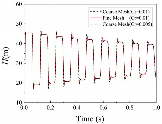
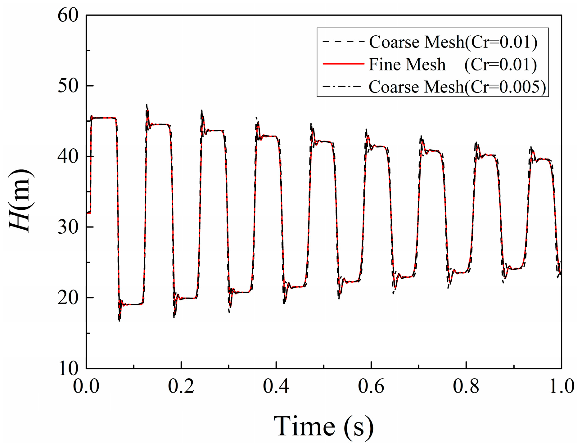
First, a mesh independence study is conducted using two cell counts: N = 50 (coarse mesh) and N = 100 (fine mesh). The influence of the Courant number (Cr) is also investigated. Based on the convergence criteria as discussed in Equations (21)–(23), two Cr values are considered: 0.01 and 0.005. The results in Figure 2 show that the solution is mesh-independent, and the Courant number has a negligible influence on the results. Furthermore, the influences of b and k′ in Equations (10)–(15) are discussed; the simulated results show that within different b and k′ values, the variation in the calculated results is negligible. Hence, b and k′ used in the calculation are taken as 1/3 and 3, respectively.

Figure 2. Mesh and Courant number independence test.

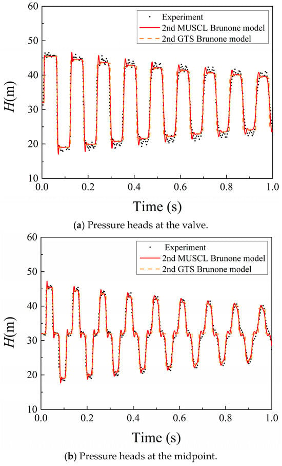
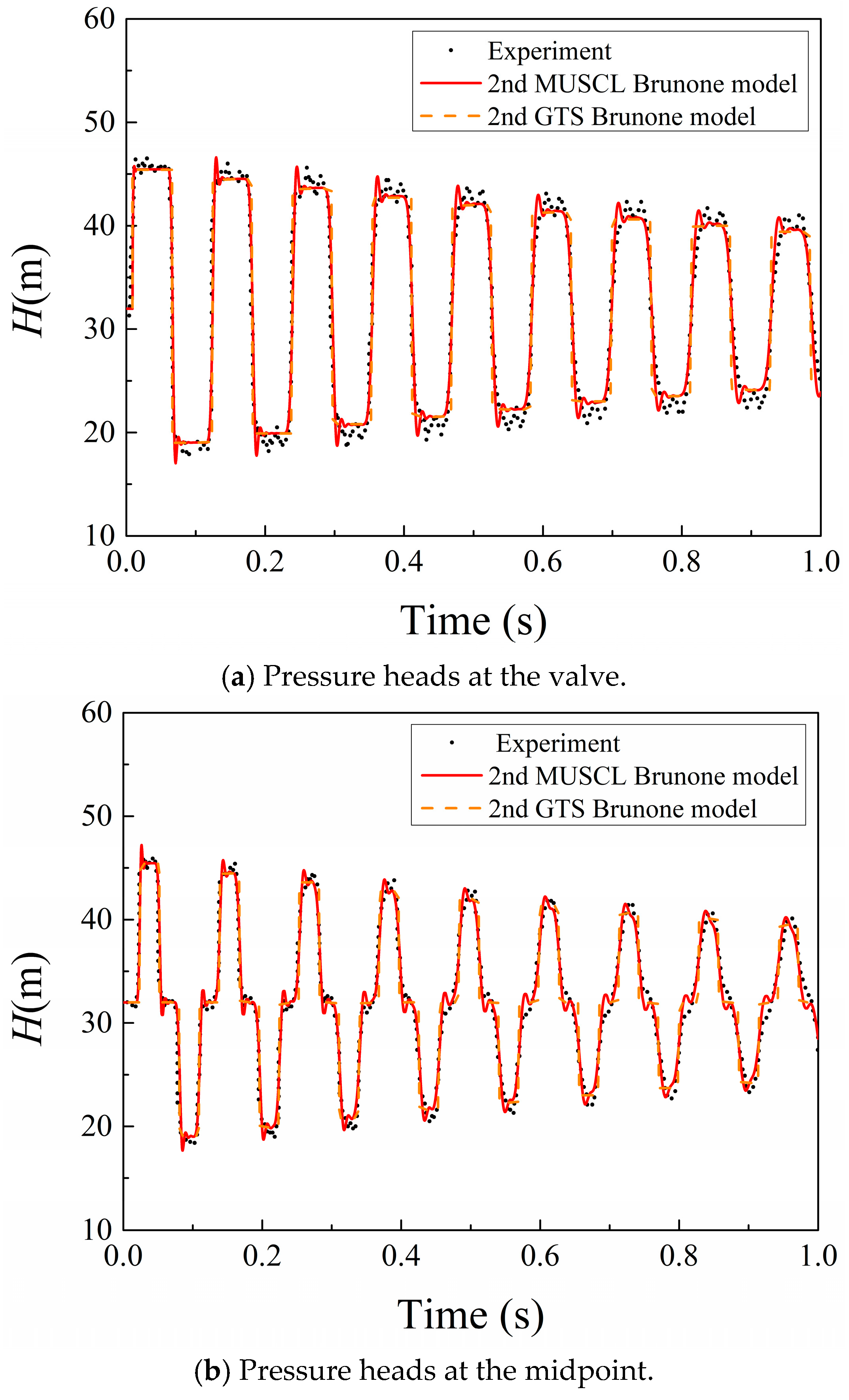
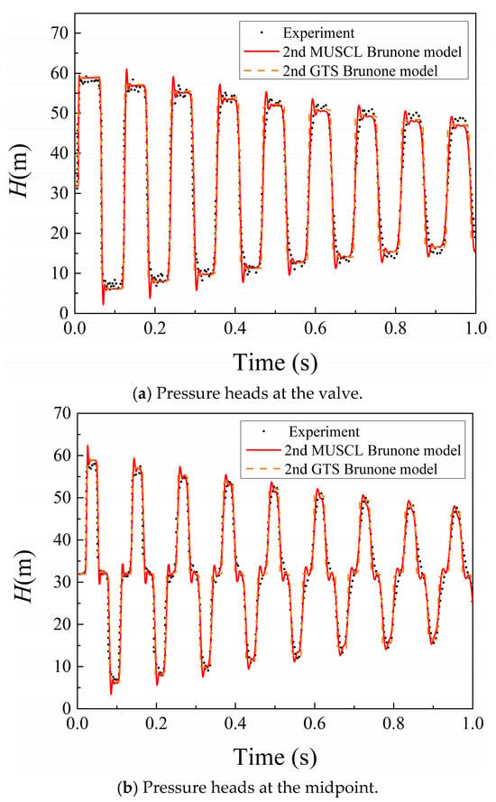
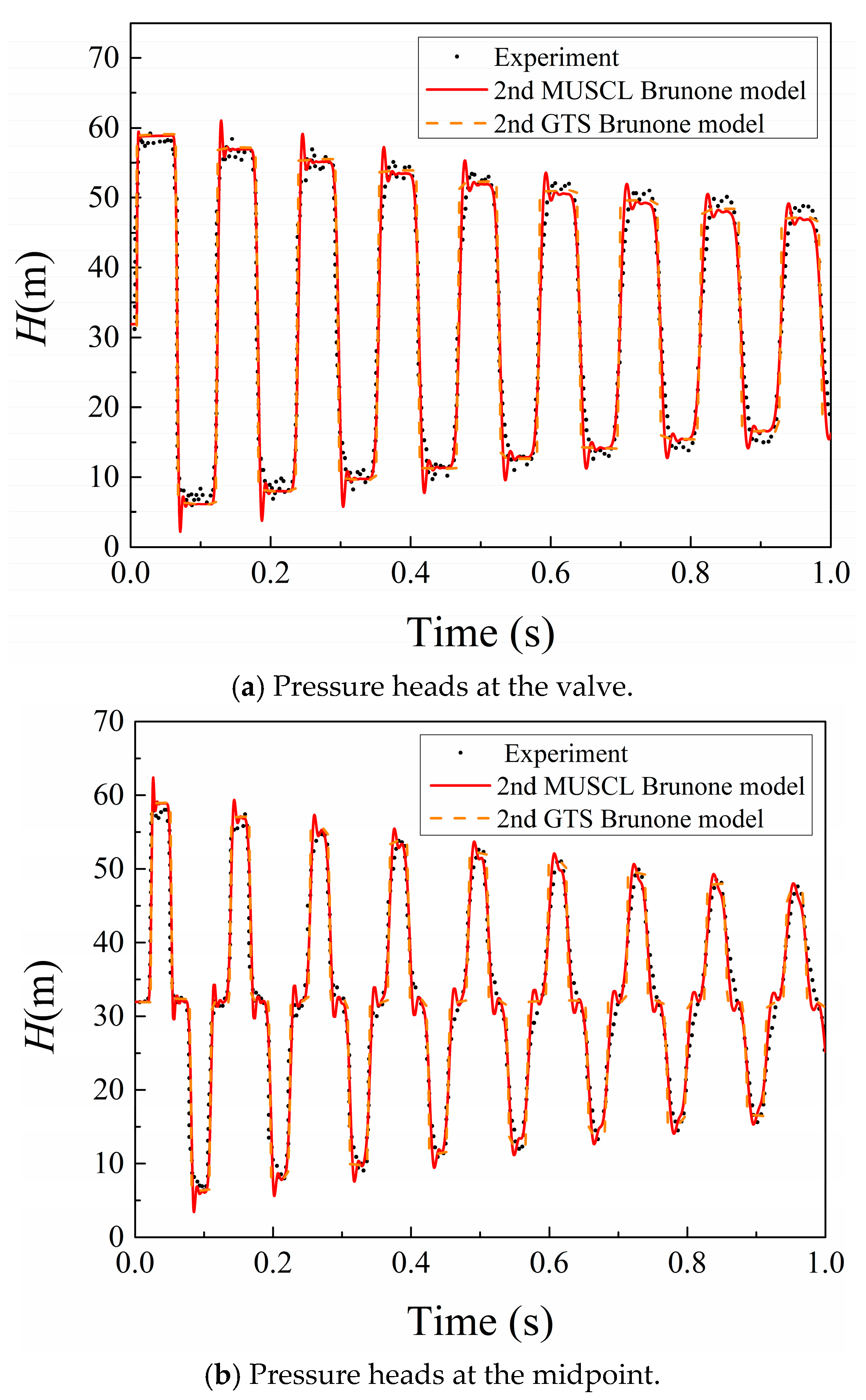
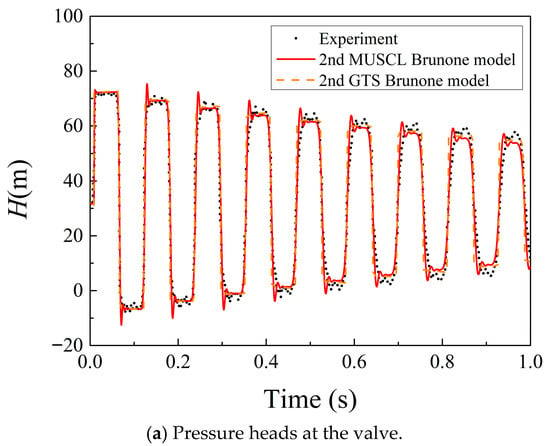
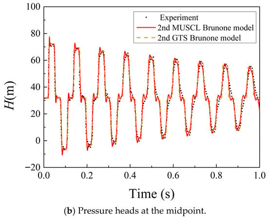
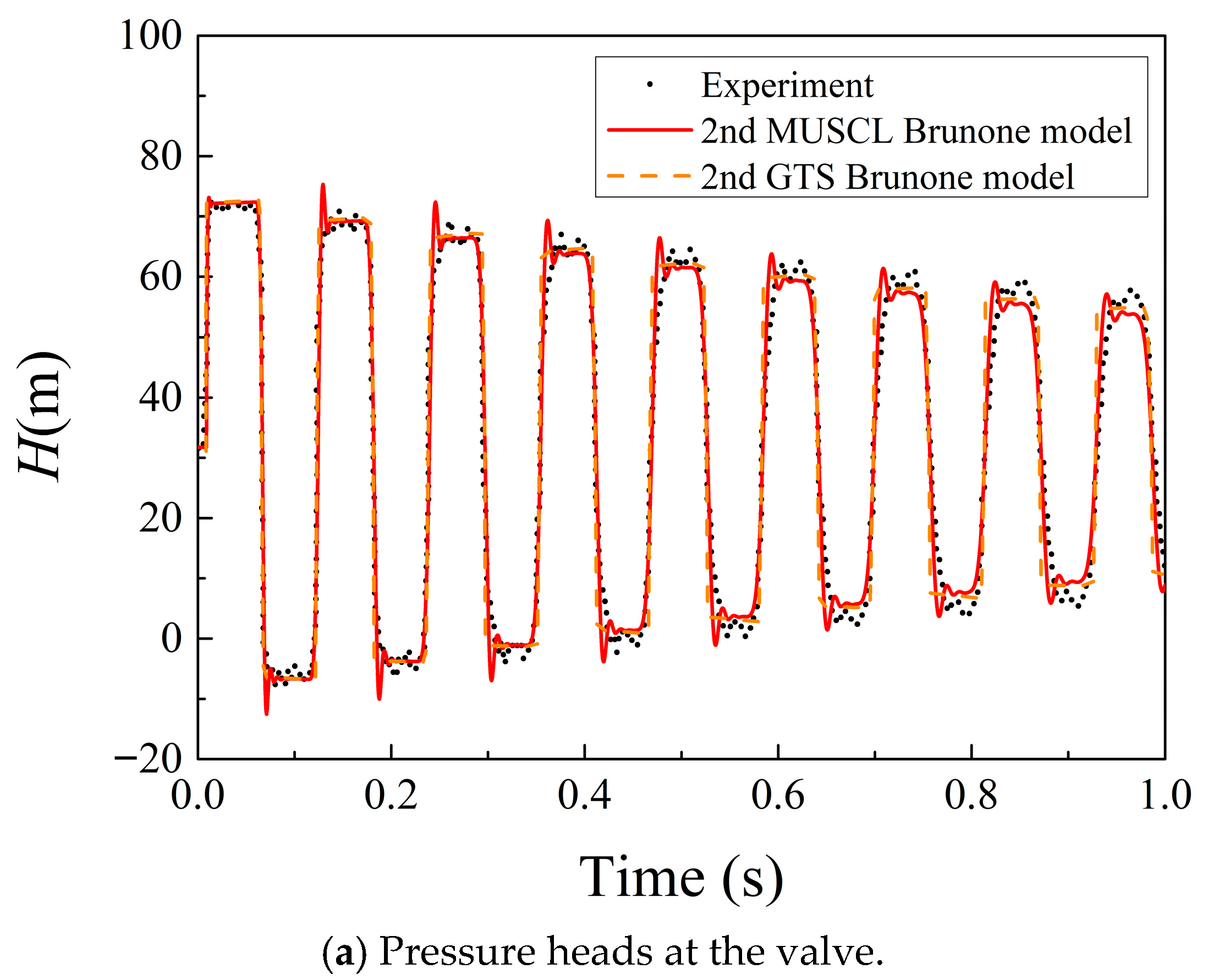
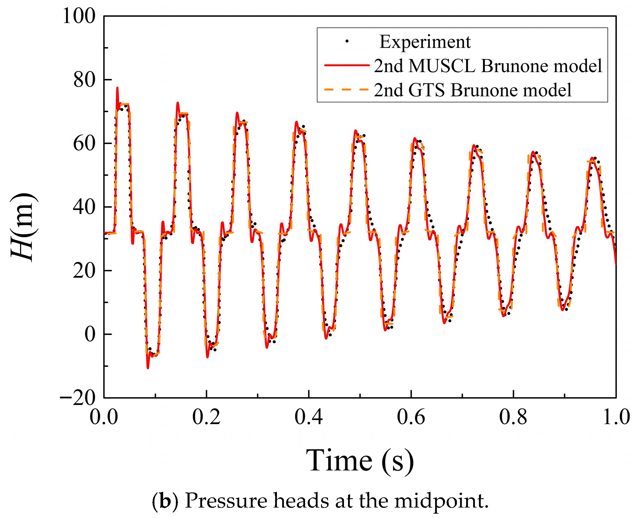
The calculations for three cases are shown in Figure 3, Figure 4 and Figure 5. For each case, the water head at two pipe positions are considered: the valve and midpoint. The numerically simulated water head is compared with the experimental results. Good agreement is observed, demonstrating sufficient simulation accuracy. The solution accuracy of the MUSCL scheme is also evaluated through a comparison with the second-order GTS in [11].

Figure 3. Initial upstream velocity equals 0.1 m/s.

Figure 4. Initial upstream velocity equals 0.2 m/s.

Figure 5. Initial upstream velocity equals 0.3 m/s.

The results confirm that calculations using both MUSCL and the GTS achieve adequate accuracy relative to the experimental data. To quantitatively assess precision, Table 1 presents the percentage error on pressure peaks (PEPP) from Figure 3, Figure 4 and Figure 5 for both methods against experimental values.

Table 1. PEPP calculated through MUSCL and GTS method.

Position	Initial Velocity	MUSCL	GTS
PEPP (At the valve)	v0 = 0.1 m/s	0.707	3.779
	v0 = 0.2 m/s	1.548	2.484
	v0 = 0.3 m/s	1.649	3.196
PEPP (At the midpoint)	v0 = 0.1 m/s	0.659	1.441
	v0 = 0.2 m/s	2.467	1.176
	v0 = 0.3 m/s	1.673	1.434

Table 1 indicates that the PEPP for both methods remains below 5%, confirming the high accuracy of the FVM approach. Notably, MUSCL yields a lower PEPP than the GTS method in most cases. Moreover, Figure 3, Figure 4 and Figure 5 demonstrate that as time evolves, MUSCL-calculated pressure peaks exhibit progressively closer agreement with the experimental measurements compared to the GTS results.

3.2. Optimal Valve Placement and Operation Strategy

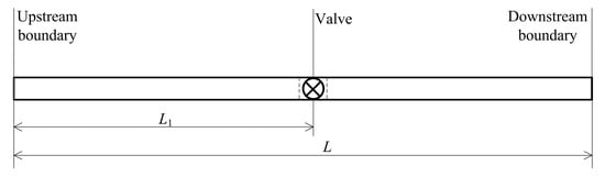
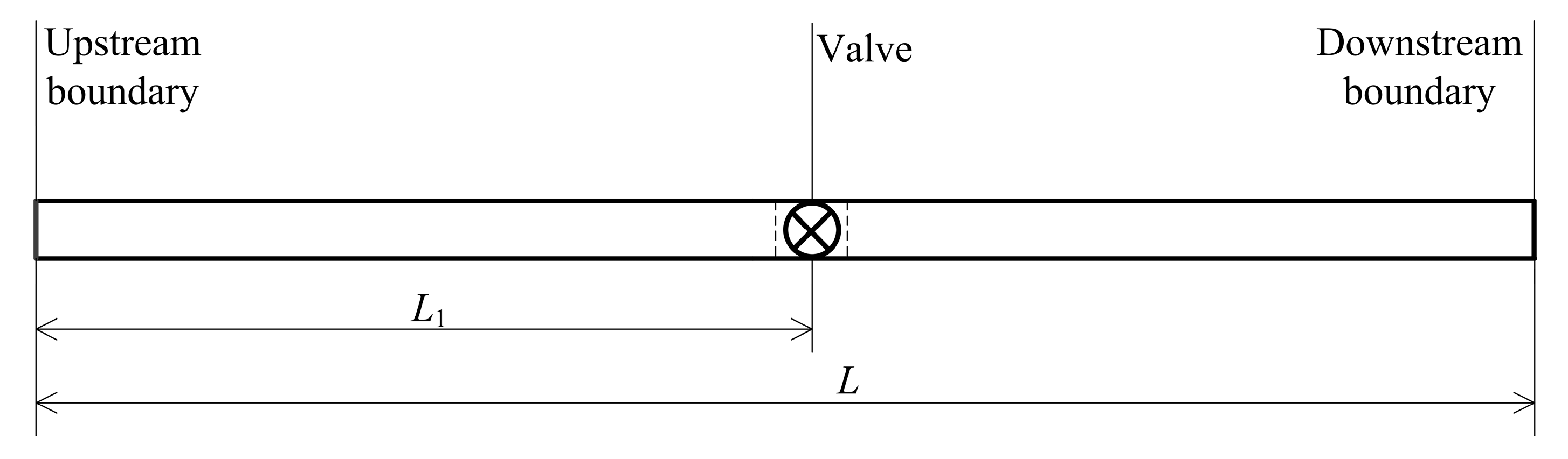
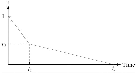
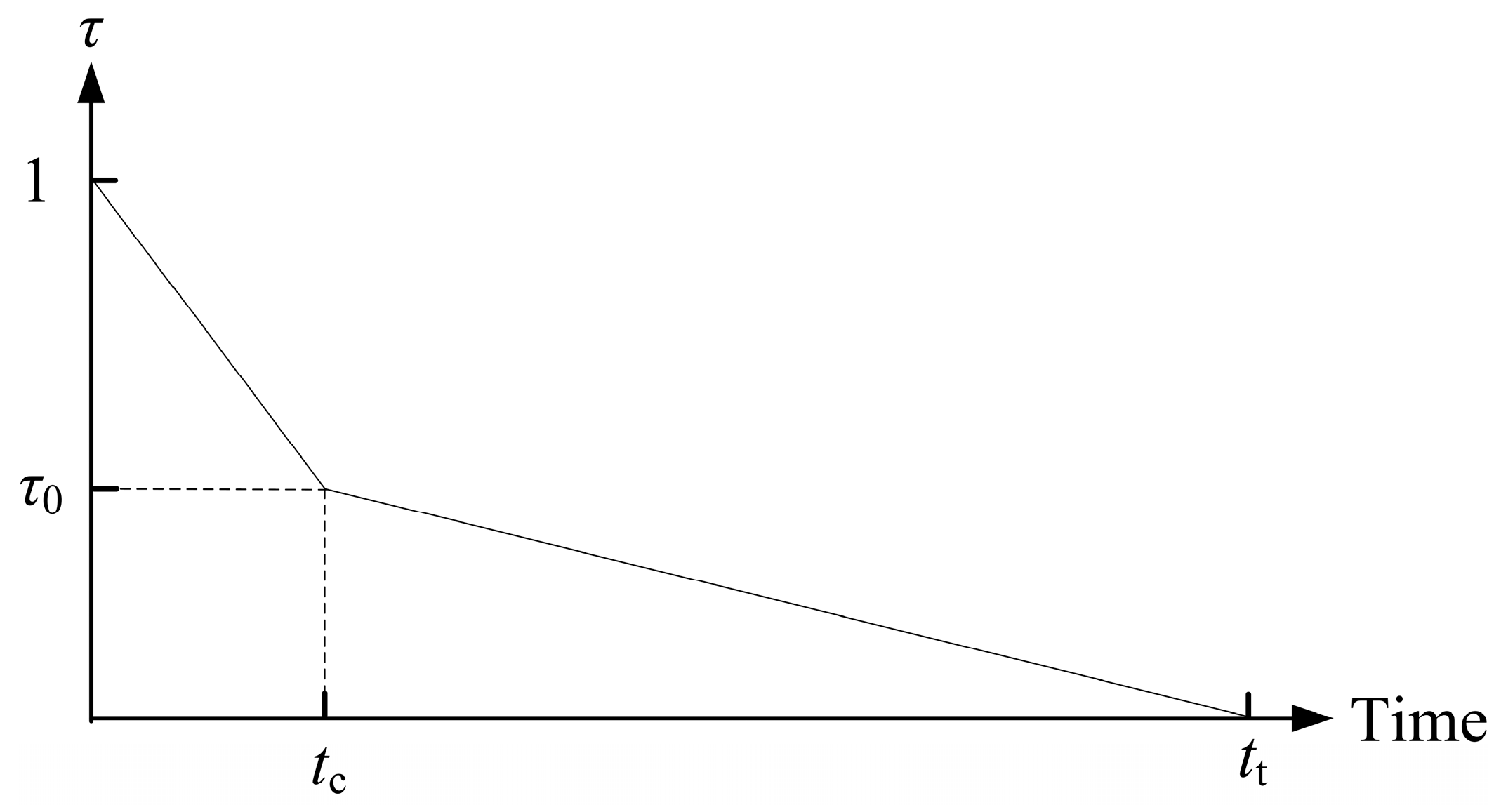
A pipeline system as shown in Figure 6 with length L = 2000 m and diameter D = 0.5 m is analyzed; the valve position (L₁) and closure regulation are optimized. Under specified inlet/outlet hydraulic heads, a two-stage closure profile as shown in Figure 7 is implemented: Stage 1 rapidly closes the valve to opening τ₀ within time t_c, while Stage 2 gradually closes it to zero over duration 4t_c. In Figure 7, τ is the valve opening, and t_t is the total valve closure time. Design variables include valve position L₁ (900 m, 1100 m), Stage 1 closure time t_c (0.5 s, 1.5 s), and intermediate opening τ₀ (0.5, 0.6).

Figure 6. The geometric layout and valve arrangement of the pipeline system.

Figure 7. The two-stage closure profile of the valve.

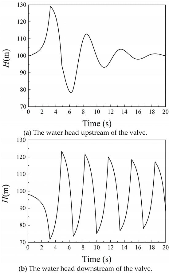
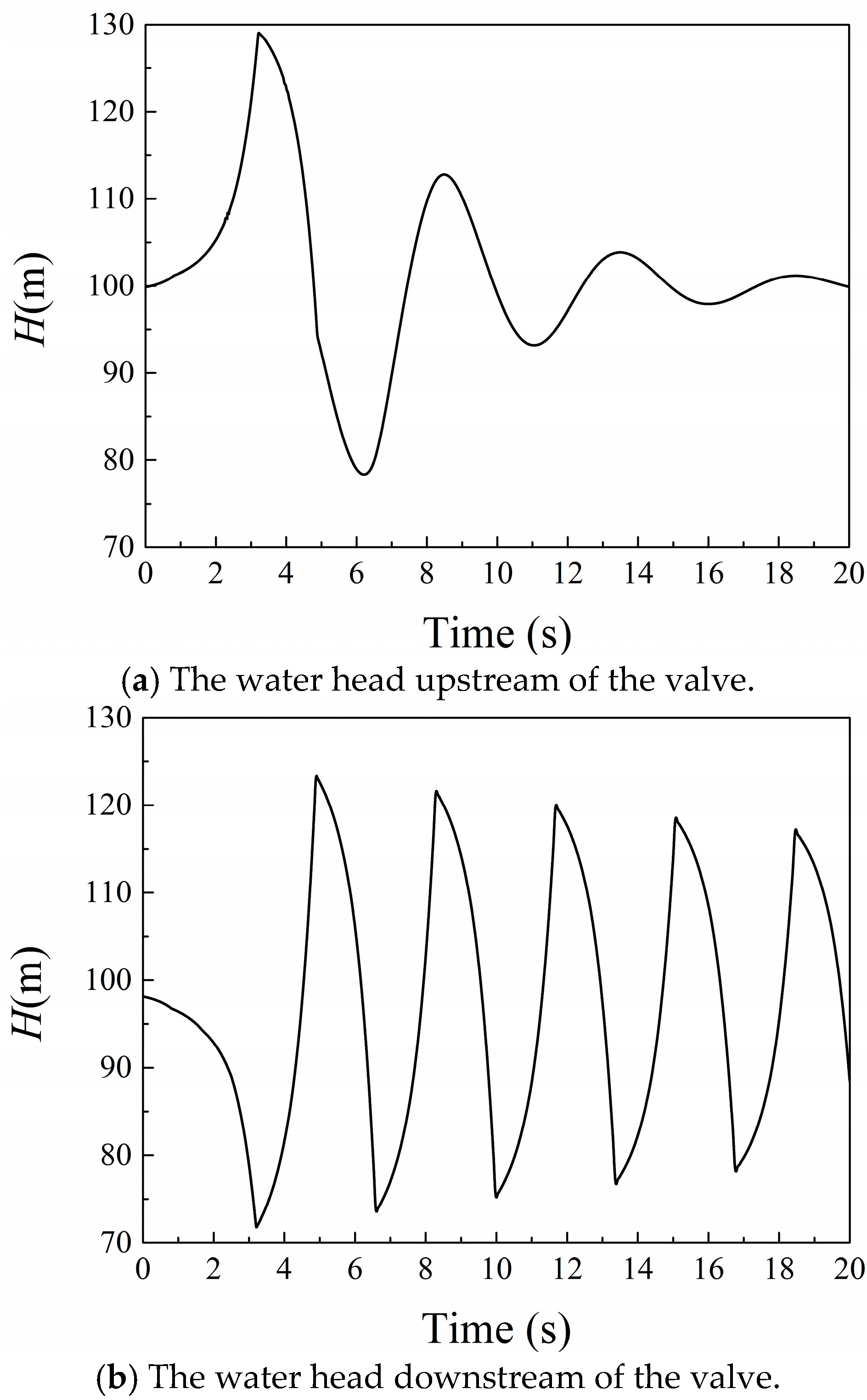
For the case (L₁ = 1000 m, t_c= 0.5 s, τ₀ = 0.6), Figure 8 demonstrates water head evolution upstream and downstream of the valve. The sudden rise in the water head during valve closure can damage pipes and lead to system failures.

Figure 8. Water head variation at valve position (case parameters: L₁ = 1000 m, t_c= 0.5 s, τ₀ = 0.6).

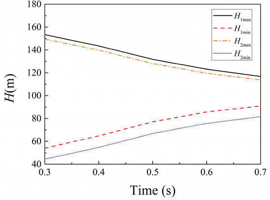
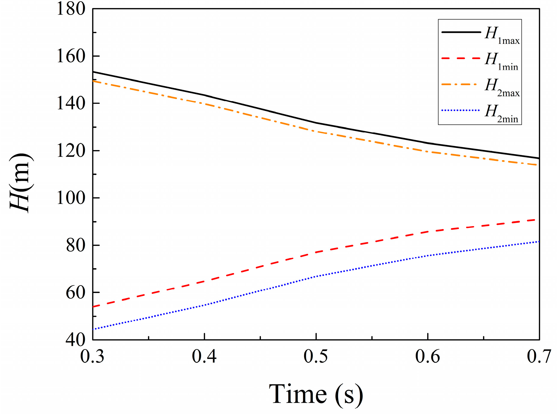
This study investigates extreme water heads at the valve: upstream maximum (H_max1), downstream maximum (H_max2), upstream minimum (H_min1), and downstream minimum (H_min2). Pipe diameter effects on these extrema are rigorously analyzed. Figure 9 quantifies the diameter dependence for the representative case (L₁ = 1000 m, tₛ = 0.5 s, τ₀ = 0.6).

Figure 9. The influence of pipe diameter on water hammer properties.

As shown in Figure 9, both H_max1 and H_max2 decrease monotonically with increasing pipe diameter, while H_min1 and H_min2 similarly increase monotonically. This indicates a reduction in the amplitude of pressure variation with larger pipe diameters. The primary mechanism is that during valve closure, the absolute decrease in flow velocity (which governs water hammer pressure) diminishes in larger pipes. Furthermore, pipe diameter enlargement can reduce wave speed. Thus, water hammer impact is mitigated. Due to this monotonic influence, a fixed pipe diameter of 0.5 m is maintained in subsequent analyses to optimize other parameters.

In this work, the influences of pipe parameters on water hammer properties are discussed using an approximate model. This model is also applied for design optimization. The parameters considered are L₁, t_c, and τ₀. The water hammer properties examined include H_max1 and H_max2; both H_max1 and H_max2 are minimized in the optimization. H_min1 and H_min2 are also considered, which are maximized in the optimization. The radial basis functions (RBF) method [31] is used to establish the approximate model as

$$F(x_d)={\displaystyle \sum _{n=1}^J{\alpha }_n{\varphi }_n(x_d)}+{\alpha }_{J+1}$$

(24)

where F(x_d) is the fitting function and x_d is the design variable vector, which includes L₁, t_c and τ₀. The sample points, $x_{dj}$, are calculated and the sampling values, $y_j$, are achieved, and then, $x_{dj}$ and $y_j$ are substituted in Equation (24), and Equation (25) is achieved as

$$\left\{\begin{array}{l}{\displaystyle \sum _{n=1}^J{\alpha }_n{\varphi }_n(x_{dj})+{\alpha }_{J+1}}=y_j,j=1,2,\dots J\\ {\displaystyle \sum _{n=1}^J{\alpha }_n}=0\end{array}\right.$$

(25)

By solving Equation (25), the unknown interpolation expansion coefficients ${\alpha }_1,{\alpha }_2,\dots ,{\alpha }_{J+1}$ can be determined, and then the approximate model is achieved. $\varphi (x)$ in Equations (24) and (25) is the radial basis function, which satisfies

$${\varphi }_j(x)={‖x-x_j‖}^c$$

(26)

where c is the shape function factor, and the range of c is (0.2, 3). In establishing the approximate model, the error between the approximation model for each sample point and the actual function value is measured, and factor c is achieved through optimization to minimize the summed errors.

An orthogonal experimental design was implemented using an L₁₂₁(11³) array, featuring 11 levels and three factors. The levels are distributed evenly in the variable ranges. This generated 121 sample cases for numerical simulation. First, sampling points are computed and their corresponding values obtained. These data points are then substituted into Equation (25) to determine the coefficients ${\alpha }_1,{\alpha }_2,\dots ,{\alpha }_{J+1}$ for each physical quantity. With the interpolation expansion coefficients established, the approximate model is constructed. The fitting accuracy of the model was verified using the $R_{\alpha }^2$ factor, with all cases exceeding 0.99. This confirms that the model possesses sufficient accuracy.

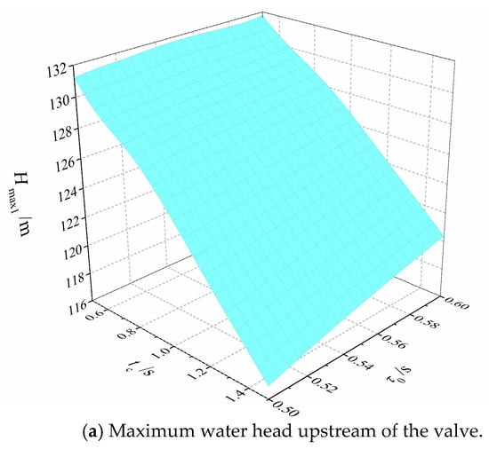
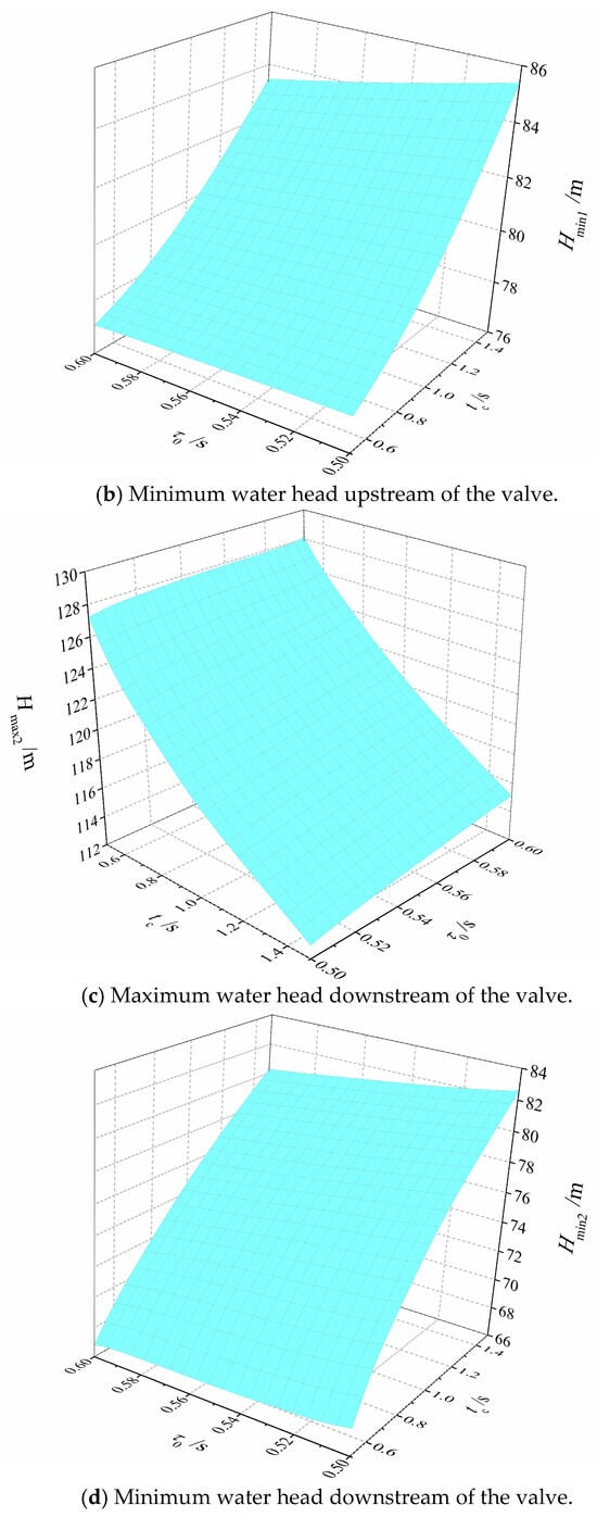
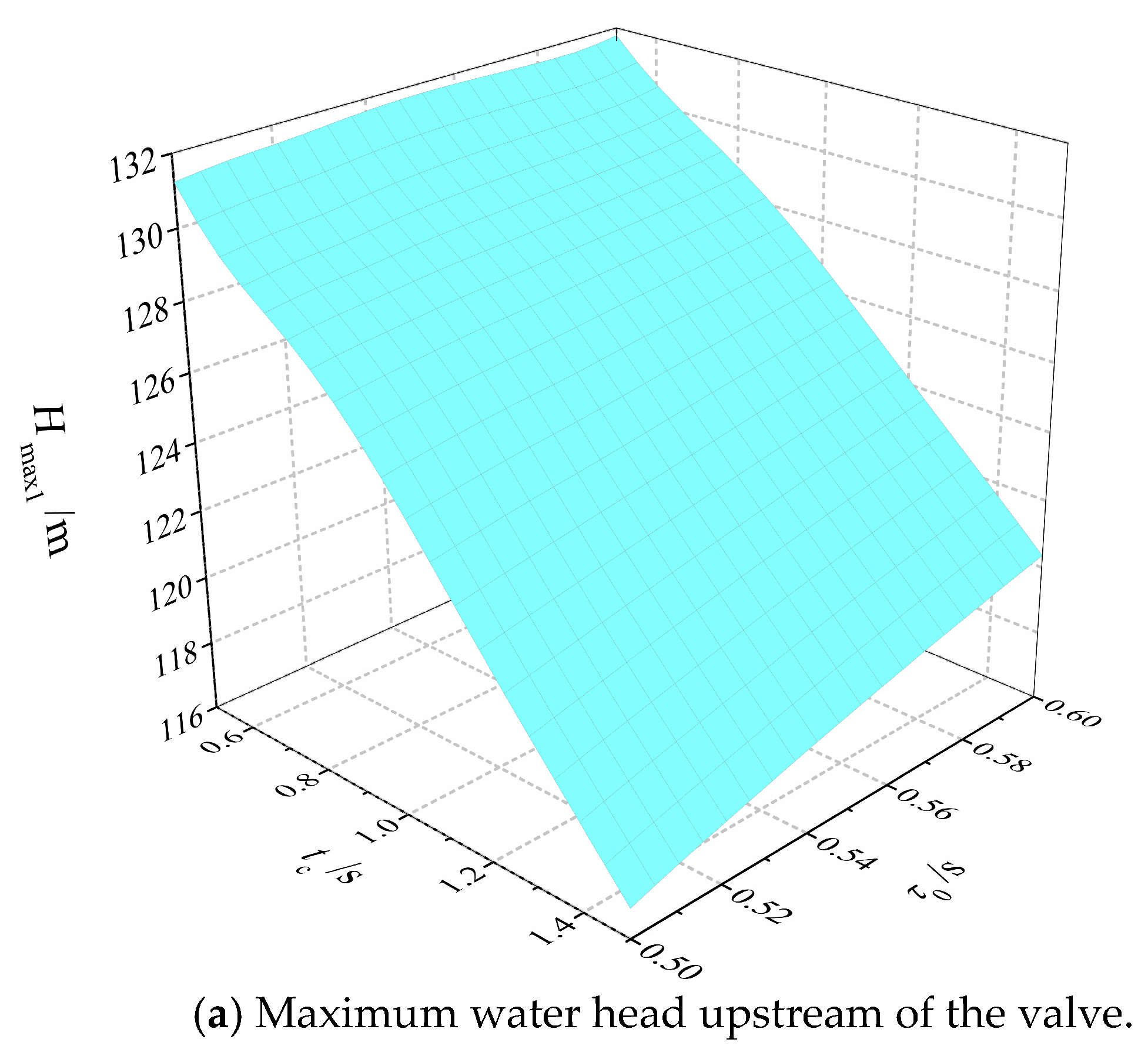
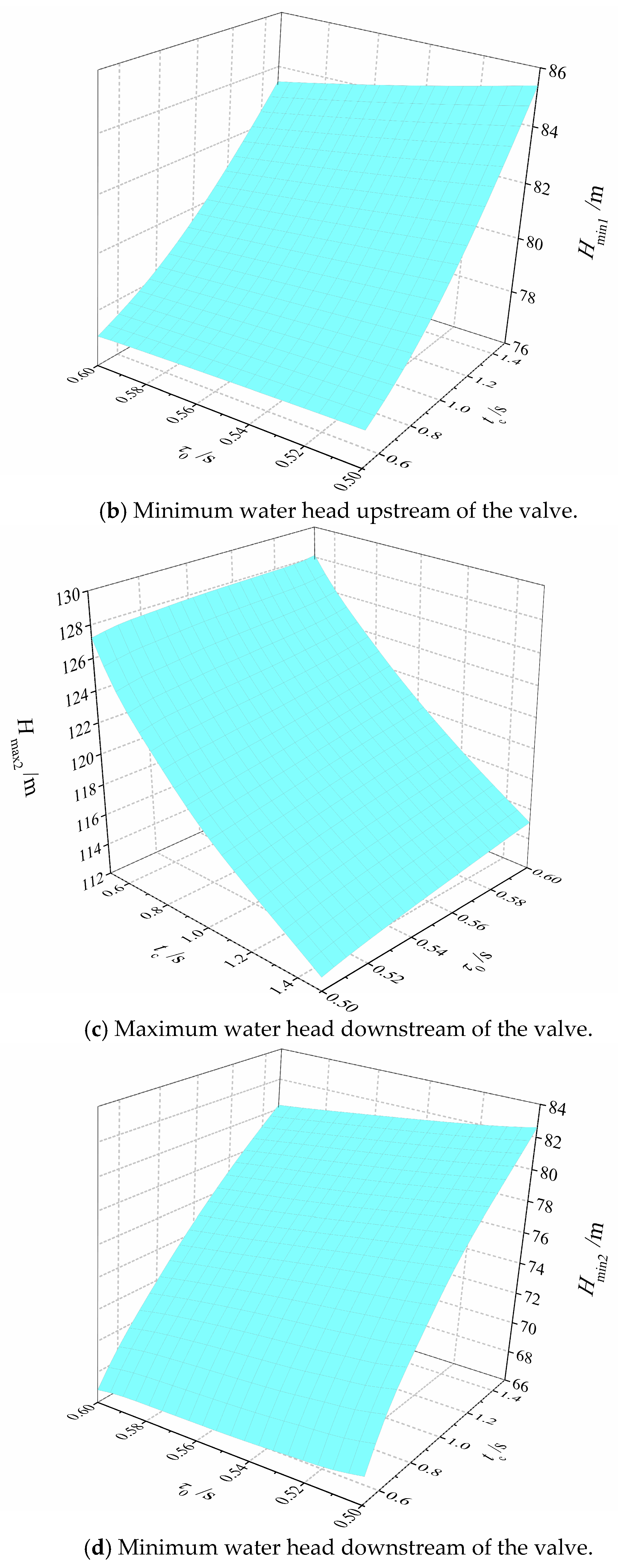
Once the approximate model is established, the influence of design parameters on water hammer properties can be analyzed. Figure 10 shows the influence of t_c and τ₀ on the maximum and minimum water head upstream and downstream of the valve when L₁ = 1000 m.

Figure 10. Extreme water head distribution across valve.

Figure 10 shows that as valve closure time t_c increases, both the maximum water head upstream and downstream of the valve decreases, while the minimum water head increases. Valve opening τ₀ also influences water head, though non-monotonically. For example, the minimum water head upstream of the valve increases with τ₀ at small t_c values but decreases with τ₀ at large t_c values. The results also indicate that L₁ exhibits non-monotonic influences. These complex relationships indicate that design optimization is necessary to determine the optimum results.

The optimization model is also established as Equation (27) to further investigate how valve operation affects water hammer properties.

$$\begin{array}{l}\min t_{\mathrm{c}}/t_{\mathrm{c}\max }+H_{\max 1}/H_{\max 1(\max )}+H_{\max 2}/H_{\max 2(\max )}-H_{\min 1}/H_{\min 1(\max )}-H_{\min 2}/H_{\min 2(\max )}\\ \mathrm{s}.\mathrm{t}. x\in E\end{array}$$

(27)

x is the design variable vector, i.e., (L₁, tₛ, τ₀), and E is the design feasible field.

A quick valve adjustment is commonly needed during pipe system operation. Hence, the optimization goal is to achieve the minimum closure time and the maximum water head while maximizing the minimum water head to avoid water hammer damage. The optimization aims to simultaneously minimize the peak water head (H_max1, H_max2), maximize the valley water head (H_min1 and H_min2) at the valve position, and minimize the valve closure time, t_c. Each objective is normalized to (0, 1) using its maximum value within the feasible design space. For instance, H_max1 is normalized by first identifying its maximum value H_max1(max) through single-objective optimization and then computing H_max1/H_max1(max). The normalized objectives are aggregated via a weighted sum with unity weights (i.e., weight = 1 per objective).

To further conduct parameter sensitivity analysis, Pareto charts are presented in this study for the approximate model, which reflect the percentage contribution of all terms in the model to each response after sample fitting. This is the standard approach in parameter sensitivity analysis research. Based on the Pareto charts, the parameter contribution percentage for parameters H_max1, H_max2, H_min1 and H_min2 is determined, respectively. The analysis results are shown in Table 2.

Table 2. Pareto chart for parameter sensitivity analysis.

	Effect of tc	Effect of L1	Effect of τ0
Hmax1	76.5%	12.5%	11.0%
Hmax2	73.2%	14.1%	12.7%
Hmin1	71.6%	18.4%	10.0%
Hmin2	73.1%	14.2%	12.7%

It can be seen in Table 2 that t_c has the largest influence on the water head; the influence of L₁ and τ₀ remains at the same level. However, all parameters should be considered in optimization due to the fact that no parameters exhibited negligible effects.

Two optimization approaches are implemented for comparative analysis. The first employs the Nonlinear Programming by Quadratic Lagrangian (NLPQL) algorithm—a gradient-based method suitable for highly nonlinear design spaces—with convergence accuracy set to 10⁻⁶. The second approach combines the Multi-Island Genetic Algorithm (MIGA), effective for locating global optima in complex design spaces, with the Hooke–Jeeves direct search algorithm. Here, MIGA provides initial values for Hooke–Jeeves refinement. Key MIGA parameters include the following: sub-population size = 20, islands = 10, and generations = 20. The optimization results from both methods exhibit less than 1% error relative to each other; consequently, Table 3 presents their results collectively. Moreover, the consistent optimum values achieved through both optimization approaches indicates robustness in the solution.

Table 3. Optimization result.

L1	τ0	tc	Hmax1	Hmax2	Hmin1	Hmin2
1100	0.5	0.56	131.03	124.46	76.84	70.61

This indicates that optimum results are achieved when the valve is located rearward of the pipeline’s midpoint, and first-stage valve opening τ₀ equals its lower boundary value. Since t_c represents valve closure time, it is minimized in the optimization to meet rapid valve adjustment requirements. However, decreasing t_c increases the water head peak. Thus, the optimization results in Table 3 reflect a balance between valve closure time and water head peak value. The optimum value of t_c = 0.56 represents the continuous solution from optimization and remains close to the prescribed lower bound of 0.5.

4. Conclusions

The influences of valve arrangement on water hammer properties are discussed. First, a second-order MUSCL-type FVM scheme is proposed for analyzing the hydraulic transient process in pipeline systems. The FVM is then adopted to analyze valve arrangement in pipes, optimizing both position and closure regulation. The following conclusions can be drawn.

The second-order MUSCL-type FVM scheme demonstrates high accuracy compared with the experimental results. The unsteady friction term is considered, and the results show that the simulation is mesh-independent and Courant number-independent. With the incorporation of the Brunone model, the second-order MUSCL scheme demonstrates superior accuracy in calculating water head peaks, yielding less than 5% error when compared to experimentally measured values.

The radial basis function (RBF) method effectively establishes approximate models for investigating water hammer characteristics and design optimization. Pipe parameter influences on hydraulic transient process can be intuitively studied through this surrogate modeling approach. This implies that sufficient sample points are required to achieve model accuracy.

When valve closure time decreases, water head in the pipe increases dramatically, indicating potential damage risk. However, modern water supply systems frequently require rapid valve adjustments. Therefore, design optimization is essential for valve arrangement. This optimization must balance adjustment time against operational safety. The results show that optimum performance is achieved when the valve is positioned rearward of the pipeline’s midpoint, and the first-stage valve opening takes a small value.

References

- Tijsseling, A.S. Water hammer with fluid-structure interaction in thick-walled pipes. Comput. Struct. 2007, 85, 844–851. [Google Scholar] [CrossRef] [Scilit]
- Plouraboué, F. Review on water-hammer waves mechanical and theoretical foundations. Eur. J. Mech. B Fluid. 2024, 108, 237–271. [Google Scholar] [CrossRef] [Scilit]
- Shu, Z.Y.; Lei, G.; Liang, W.Q.; Huang, L.; Che, B.X.; Zheng, X.H.; Qian, H. Rapid prediction of water hammer characteristics in liquid hydrogen storage and transportation systems: A Theoretical model. Renew. Energy 2024, 230, 120781. [Google Scholar] [CrossRef] [Scilit]
- Liu, Z.; Yu, X.D.; Pérez-Díaz, J.I.; Liu, Y.; Martínez-Lucas, G. Influence of water hammer effect on low frequency oscillation of Grid-connected hydropower station system. Renew. Energy 2023, 219, 119530. [Google Scholar] [CrossRef] [Scilit]
- Adel, M.; Kassem, F.A.M.; Fathy, I. Reducing the water hammering, surges, and slamming caused by check valve closure in a wastewater pumping station by using a swing flex check valve. Flow Meas. Instrum. 2025, 104, 102870. [Google Scholar] [CrossRef] [Scilit]
- Wylie, E.B.; Streeter, V.L. Fluid Transients, 1st ed.; McGraw-Hill: New York, NY, USA, 1978. [Google Scholar]
- Lian, J.J.; Yang, X.W.; Wang, H.J. Propagation characteristics analysis of high-frequency vibration in pumped storage power station based on a 1D fluid-solid coupling model. J. Energy Storage 2023, 68, 107869. [Google Scholar] [CrossRef] [Scilit]
- Wu, G.H.; Zhu, J.H.; Han, H.; Liu, Z.K.; Li, X.Q.; Tang, X.L. Dynamics of large cavity induced by valve closure in an undulating pipeline. Phys. Fluids 2023, 35, 123312. [Google Scholar] [CrossRef] [Scilit]
- Zhao, M.; Ghidaoui, M.S. Godunov-type solutions for water hammer flows. J. Hydraul. Eng. 2004, 130, 341–348. [Google Scholar] [CrossRef] [Scilit]
- Zhou, L.; Wang, H.; Liu, D.Y.; Ma, J.J.; Wang, P.; Xia, L. A second-order finite volume method for pipe flow with water column separation. J. Hydro-Environ. Res. 2017, 17, 47–55. [Google Scholar] [CrossRef] [Scilit]
- Zhou, L.; Li, Y.J.; Karney, B.; Cheng, Y.G.; Liu, D.Y. Godunov-type solutions for transient pipe flow implicitly incorporating Brunone unsteady friction. J. Hydraul. Eng. 2021, 147, 04021021. [Google Scholar] [CrossRef] [Scilit]
- Zhou, L.; Li, Y.J.; Zhao, Y.; Ou, C.Q.; Zhao, Y. An accurate and efficient scheme involving unsteady friction for transient pipe flow. J. Hydroinform. 2021, 23, 879–896. [Google Scholar] [CrossRef] [Scilit]
- Li, H.Y.; Zhang, Y.; Cui, J.G.; Zhang, F.; Yang, X.Y.; Shi, W.T.; Mao, L.B. Optimization of water hammer protection against sudden pump stoppage using machine learning models and intelligent algorithms. J. Hydraul. Res. 2025, 63, 265–277. [Google Scholar] [CrossRef] [Scilit]
- Yazdi, J.; Hokmabadi, A.; JaliliGhazizadhe, M.R. Optimal size and placement of water hammer protective devices in water conveyance pipelines. Water Resour. Manag. 2019, 33, 569–590. [Google Scholar] [CrossRef] [Scilit]
- Henclik, S. Numerical modeling of water hammer with fluid-structure interaction in a pipeline with viscoelastic supports. J. Fluid. Struct. 2018, 76, 469–487. [Google Scholar] [CrossRef] [Scilit]
- Li, R.; Gao, Y.Q.; Jiang, B.Y.; Lv, M.; Li, H. Intelligent parameter optimization of sealed airbag vessels with preventing water hammer in cascaded pressurized water transmission system: Based on MOPSO algorithm. J. Water Process Eng. 2025, 70, 106915. [Google Scholar] [CrossRef] [Scilit]
- Ma, J.; Wu, J.D.; Wang, X.D. Simulation of computation and experimental investigations about water hammer in high lift water transmission pipeline. In Proceedings of the International Conference on Advances in Mechanical Engineering and Industrial Informatics, Zhengzhou, China, 11–12 April 2015. [Google Scholar]
- Xin, Q.L.; Du, J.Y.; Liu, M.; Liu, Y.; Huang, J.K.; Yu, W.; Yuan, F.Y.; Wang, D.X.; Yang, X.J. Experimental study on the effects of two-stage valve closure on the maximum water hammer pressure in micro-hydroelectric system. J. Water Process Eng. 2024, 65, 105886. [Google Scholar] [CrossRef] [Scilit]
- Yao, E.; Kember, G.; Hansen, D. Analysis of water hammer attenuation in applications with varying valve closure times. J. Eng. Mech. 2015, 141, 04014107. [Google Scholar] [CrossRef] [Scilit]
- Wang, P.; Yu, J. Numerical simulation of water hammer boundary conditions based on nozzle outflow law. J. Drain. Irrig. Mach. Eng. 2020, 38, 814–818. [Google Scholar]
- Van Leer, B. Towards the Ultimate Conservative Difference Scheme. V. A Second-order Sequel to Godunov’s Method. J. Comput. Phys. 1979, 32, 101–136. [Google Scholar] [CrossRef] [Scilit]
- Zhao, J.H.; Özgen-Xian, I.; Liang, D.F.; Wang, T.; Hinkelmann, R. An improved multislope MUSCL scheme for solving shallow water equations on unstructured grids. Comput. Math. Appl. 2019, 77, 576–596. [Google Scholar] [CrossRef] [Scilit]
- Leveque, R.J. Finite Volume Methods for Hyperbolic Problems, 1st ed.; World Publishing Beijing Corporation Limited: Beijing, China, 2004. [Google Scholar]
- Sohn, S.I. A new TVD-MUSCL scheme for hyperbolic conservation laws. Comput. Math. Appl. 2005, 50, 231–248. [Google Scholar] [CrossRef] [Scilit]
- Hou, J.M.; Liang, Q.H.; Zhang, H.B.; Hinkelmann, R. Multislope MUSCL method applied to solve shallow water equations. Comput. Math. Appl. 2014, 68, 2012–2027. [Google Scholar] [CrossRef] [Scilit]
- Guinot, V.; Delenne, C. MUSCL schemes for the shallow water sensitivity equations with passive scalar transport. Comput. Fluids 2012, 59, 11–30. [Google Scholar] [CrossRef] [Scilit]
- Leng, Y.; Li, X.L.; Fu, D.X.; Ma, Y.W. Optimization of the MUSCL scheme by dispersion and dissipation. Sci. China Phys. Mech. 2012, 55, 844–853. [Google Scholar] [CrossRef] [Scilit]
- Hubbard, M.E. Multidimensional slope limiters for MUSCL-type finite volume schemes on unstructured grids. J. Comput. Phys. 1999, 155, 54–74. [Google Scholar] [CrossRef] [Scilit]
- Toro, E.F. Riemann Solvers and Numerical Methods for Fluid Dynamics, 3rd ed.; Springer: Berlin/Heidelberg, Germany, 2009. [Google Scholar]
- Bergant, A.; Simpson, A.R.; Vìtkovsk, J. Developments in unsteady pipe flow friction modeling. J. Hydraul. Res. 2001, 39, 249–257. [Google Scholar] [CrossRef] [Scilit]
- Li, Y.F.; Yin, Y.H.; Yang, H.; Liu, X.E.; Mo, J.; Cui, H.L. Modeling for Optimization of Circular Flat Pad Aerostatic Bearing with A Single Central Orifice-Type Restrictor Based on CFD Simulation. Tribol. Int. 2017, 109, 206–216. [Google Scholar] [CrossRef] [Scilit]
Disclaimer/Publisher’s Note: The statements, opinions and data contained in all publications are solely those of the individual author(s) and contributor(s) and not of MDPI and/or the editor(s). MDPI and/or the editor(s) disclaim responsibility for any injury to people or property resulting from any ideas, methods, instructions or products referred to in the content. |
© 2025 by the authors. Licensee MDPI, Basel, Switzerland. This article is an open access article distributed under the terms and conditions of the Creative Commons Attribution (CC BY) license (https://creativecommons.org/licenses/by/4.0/).