A Multi-Model Sensitivity Analysis Framework for Environmental-Factor-Driven Atmospheric CO₂ Variations Based on Ground-Based Raman Lidar Observations

Abstract

Atmospheric CO₂ variations at regional scales reflect boundary-layer mixing, meteorological conditions, and combustion-related emissions, yet their relative contributions remain difficult to separate with single-model analyses. This study develops a multi-model framework for ground-based Raman lidar observations in Nanyang, Henan Province, integrating physically inspired diffusion and mixing proxies, an XGBoost/Ensemble attribution model, a physics-guided gradient-regularized neural network (PG-GRNN), and Granger time-predictability testing. The analysis used 22,942 quality-controlled samples and vertically averaged CO₂ concentrations from 210 to 600 m. The multi-model comparison identified pressure, temperature, humidity, NO₂, and SO₂ as the most consistent factors associated with CO₂ variability. Granger analysis further showed significant lagged predictive relationships for NO₂, pressure, SO₂, temperature, and humidity, with optimal lag orders of 2, 9, 9, 7, and 10, respectively. PG-GRNN reached high prediction accuracy (R² = 0.9744; MSE = 15.41), while the complete comparison showed that temporal predictability, physics-guided learning, and physically inspired proxies captured complementary aspects of the CO₂ response. The framework provides an interpretable route for combining ground-based lidar, environmental monitoring, and time-series analysis to support regional carbon monitoring and remote-sensing product validation.

1. Introduction

Atmospheric carbon dioxide (CO₂) has increased continuously and affected the global climate system [1]. Regional CO₂ concentrations reflect anthropogenic emissions, atmospheric transport and environmental conditions. Separating these influences requires observations that resolve local variations and analytical methods that distinguish their different associations with CO₂. Recent satellite lidar and hyperspectral studies have advanced carbon monitoring from global XCO₂ retrieval to facility-scale CO₂ and greenhouse-gas emission estimation [2,3,4,5]. Ground-based profile observations provide complementary temporal and vertical information for investigating local CO₂ variability and its environmental drivers. The existing methods for analyzing CO₂-concentration driving factors mainly include physical transport diffusion models, machine-learning algorithms, and statistical analysis methods [6,7,8,9,10,11]. Among them, physical models (such as Gaussian plume models and box models) are based on fundamental physical laws such as mass conservation and describe the processes of atmospheric transport, mixing, and diffusion parametrically, providing theoretical basis for CO₂ transport process simulation. However, due to the uncertainty in the parameterization process of the models and the obvious scale dependence and spatial heterogeneity of atmospheric processes, their application at regional-to-global scales still has certain limitations. In recent years, data-driven methods represented by neural networks and ensemble learning can learn the nonlinear relationship between variables and CO₂ concentration based on observational data and be applied to CO₂-concentration change simulation and emission inversion studies [12,13,14,15,16,17,18,19,20,21]. However, due to the lack of clear physical constraints, their model structures and prediction processes are often difficult to explain, and the physical consistency of their prediction results still needs to be further analyzed and verified [22,23,24,25,26,27,28]. Traditional statistical regression and correlation analysis methods have advantages such as simple structure and strong interpretability, but their ability to handle complex nonlinear relationships and collinearity among variables is still limited. Therefore, existing methods still have limitations in CO₂-concentration prediction, environmental factor contribution analysis, and physical interpretation. It is necessary to explore a comprehensive analysis framework that integrates multiple methods.

Based on the above analysis, the current research on CO₂ driving factors mainly faces two challenges. (1) Uncertainty in contribution assessment due to differences between models: Since different models are based on different theoretical assumptions and feature-extraction mechanisms, the sensitivity-analysis results of environmental factors may vary [29,30]. For example, physical process models usually emphasize the important role of weakened vertical turbulent exchange under stable stratification conditions on CO₂ accumulation, while machine-learning models may reveal a strong statistical correlation between ground pressure and CO₂ changes. The resulting model dependence may increase the uncertainty in driving factor identification and contribution assessment. (2) The problem of mismatch in timescales of multiple data sources: Due to the different time resolutions of ground-based or satellite observation data, reanalysis data, and numerical model outputs, the analysis of relationships between variables at different timescales is limited [31]. In addition, the lagging influence of environmental factors on CO₂-concentration changes still lacks systematic analysis. Therefore, a multi-model framework integrating physical models, data-driven methods, and statistical analysis needs to be explored to improve the reliability of CO₂ change attribution and prediction.

Using high-resolution ground-based CO₂ observations together with meteorological parameters, pollutant concentrations, and other environmental variables, this study builds a multi-model collaborative analysis framework. The framework integrates PG-GRNN, physically inspired diffusion and mixing proxies, the XGBoost/Ensemble attribution model, and Granger time-predictability testing. PG-GRNN constrains the gradient response of model output to environmental inputs, the ensemble model captures nonlinear relationships, and the Granger test evaluates whether historical environmental information improves CO₂ prediction at different lag orders. Together, these methods assess environmental contributions and time-response characteristics for regional CO₂ variation.

2. Research Area, Data and Methods

2.1. Overview of the Study Area

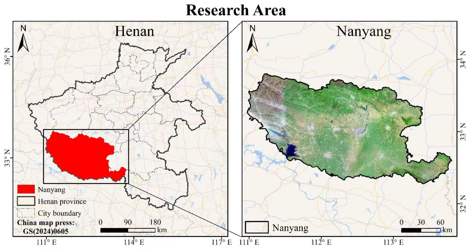
This study was conducted at the Henan Province Engineering Research Center of Environmental Laser Remote Sensing Technology and Application in Nanyang City, Henan Province. The study area is shown in Figure 1. The center is equipped with CO₂ lidar cabins, aerosol lidar systems, and micrometeorological stations, which can simultaneously acquire vertical optical and physical aerosol properties; CO₂ profiles; and meteorological elements such as temperature, pressure, humidity, and wind speed. The study area is located in the Qinling–Huaihe climate boundary zone, a transition zone between the subtropical monsoon climate and the warm temperate monsoon climate, with distinct monsoon characteristics. The annual average temperature is approximately 15 °C, and annual precipitation is about 803.3 mm. Precipitation is mainly concentrated in summer, with seasonal variation characterized by hot, humid summers and cold, dry winters.

Figure 1. Location of the study area in Nanyang, Henan Province, China.

In recent years, with the development of regional economy, the intensification of industrial activities, and the adjustment of energy consumption structure, Nanyang City has faced the dual demands of improving air environmental quality and managing carbon emissions. Conducting research on the characteristics of regional CO₂-concentration changes and their environmental driving factors is helpful for understanding the carbon cycle process at the urban and regional scales. At the same time, the complex meteorological conditions and underlying surface features in the Nanyang area may affect the interpretation of CO₂-concentration changes and their driving mechanisms. The CO₂-concentration changes in this area are influenced by multiple factors such as meteorological conditions, regional emissions, and atmospheric transport processes.

2.2. Multi-Source Observation Data and Preprocessing

This study used ground-based high-resolution hyperspectral Raman lidar observations, ground environmental monitoring, and meteorological auxiliary data to construct a dataset for analyzing regional atmospheric CO₂ variation. The observation system continuously acquired vertical CO₂ profiles, while ground-monitoring instruments simultaneously recorded near-surface pollutant concentrations and meteorological parameters. To ensure comparability among data sources in the subsequent model analysis, the data were time-synchronized, quality-controlled, screened for outliers, and matched across scales to form a unified environmental-variable input dataset. The following sections introduce the CO₂ profile observation system, inversion method, environmental monitoring data, and multi-source preprocessing workflow.

2.2.1. Hyperspectral Raman Lidar CO₂ Observation System

This study conducted field observations using a modular integrated observation platform. The cabin interior integrates a high-resolution CO₂ hyperspectral Raman lidar system, a data acquisition and control module, and operation support equipment, enabling continuous automatic observations. The lidar system is mainly composed of the laser emission part, the optical receiving part, and the system control part. The top of the cabin is equipped with a three-dimensional rotating scanning platform, with horizontal and vertical scanning ranges of 0° to 360° and 0° to 180° respectively, allowing for multi-directional atmospheric detection.

In addition, a miniature meteorological station was installed outside the observation cabin and operated synchronously with the Raman lidar. The meteorological measurements were temporally matched to the corresponding lidar observations and used as ancillary data for CO₂ profile inversion and the analysis of environmental driving factors. Table 1 summarizes the main technical specifications of the Raman lidar system used in this study.

Table 1. Main specifications of the Raman lidar system.

Parameter Category	Parameter Name	Technical Parameter Value
Laser Emission System	Laser type	Q-switched Nd:YAG Laser
	Wavelength	355 nm
	Pulse energy	40 mJ
	Repetition rate	10 Hz
Optical Receiving System	Telescope configuration	Coaxial transmitter–receiver telescope system
	Aperture	300 mm
Signal Acquisition System	Number of detection channels	3
	Vertical resolution	30 m or 15 m (This study selected 30 m)
	Temporal resolution	1 min

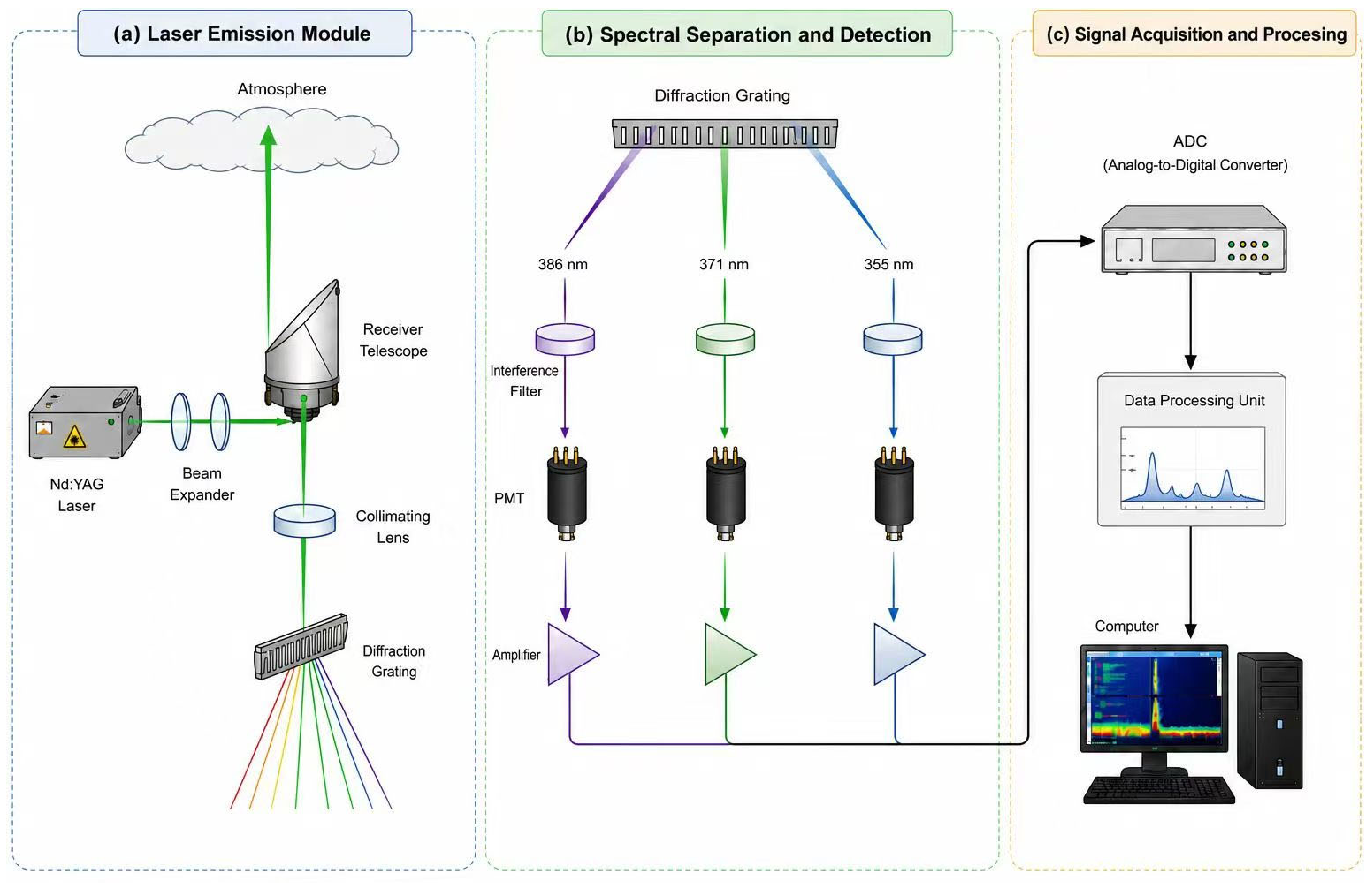
The hyperspectral-resolution Raman lidar employs a tri-doubled Nd:YAG laser as the emission source, with an output wavelength of 355 nm for narrow-linewidth ultraviolet pulsed laser. The laser passes through beam expansion, collimation, and reflection optical path adjustments before being emitted perpendicularly into the atmosphere. During its propagation, the laser beam interacts with atmospheric aerosols, air molecules, and components such as N₂, generating elastic backscattering signals and inelastic Raman scattering signals. Among them, the 355 nm elastic backscattering signal mainly reflects the Mie scattering characteristics of aerosols, while the Raman scattering signals of CO₂ and N₂ are obtained separately from the corresponding spectral channels.

The backscattering signal is collected by a Schmidt–Cassegrain telescope with a 300 mm aperture, which then passes through a small aperture diaphragm, a collimating mirror, and a narrowband filter, and is separated into the aerosol Mie scattering channel, the CO₂ Raman scattering channel, and the N₂ Raman scattering channel. The signals of each channel are detected by a photomultiplier tube (PMT), amplified, and digitized before being recorded to a computer, forming digital profile data. Subsequently, the system performs CO₂-concentration inversion based on the ratio of CO₂ and N₂ Raman signal intensities to reduce system response variations and uncertainties caused by the atmospheric transmission process. The overall structure of the lidar, and the signal acquisition and processing flow are shown in Figure 2.

Figure 2. Schematic of the high-spectral-resolution Raman lidar system. The arrows indicate the direction of optical propagation, electronic signal transmission, and data flow. The spectra shown in the Data Processing Unit and Computer are schematic illustrations of the signal processing stages, not actual running screenshots.

2.2.2. Method for Inversion of CO₂-Concentration Profiles

Raman lidar CO₂ profile inversion is based on the inelastic backscattering characteristics of atmospheric molecules. Since the volume fraction of nitrogen (N₂) in the atmosphere is relatively stable (approximately 78%), its Raman scattering signal can be used as an internal reference signal for CO₂ inversion process. By calculating the ratio of the Raman signal intensities of CO₂ and N₂, the influence of laser energy fluctuations, system variations, and partial atmospheric transmission errors on the inversion results can be weakened.

For the Raman scattering signals of CO₂ and N₂ received at a range height, z, their echo powers satisfy the Raman lidar equation. If $P_{{\mathsf{\lambda }}_C}\left(z\right)$ and $P_{{\mathsf{\lambda }}_N}\left(z\right)$ represent the received optical power at the characteristic Raman scattering wavelengths of CO₂ and N₂, respectively, the echo powers can be expressed as follows:

$$P_{{\mathsf{\lambda }}_C}\left(z\right)=K_C\cdot {\displaystyle \frac{{\mathsf{\gamma }}_C\left(z\right)}{z^2}}\cdot {\mathsf{\beta }}_C\left(\mathsf{\pi }\right)\cdot N_C\left(z\right)\cdot T\left(z,{\mathsf{\lambda }}_0,{\mathsf{\lambda }}_C\right)$$

(1)

$$P_{{\mathsf{\lambda }}_N}\left(z\right)=K_N\cdot {\displaystyle \frac{{\mathsf{\gamma }}_N\left(z\right)}{z^2}}\cdot {\mathsf{\beta }}_N\left(\mathsf{\pi }\right)\cdot N_N\left(z\right)\cdot T\left(z,{\mathsf{\lambda }}_0,{\mathsf{\lambda }}_N\right)$$

(2)

In Equations (1) and (2), $K_C$ and $K_N$ are channel-specific system constants that include emitted laser power and detection efficiency. The functions ${\mathsf{\gamma }}_C\left(z\right)$ and ${\mathsf{\gamma }}_N\left(z\right)$ describe channel overlap. The terms ${\mathsf{\beta }}_C\left(\mathsf{\pi }\right)$ and ${\mathsf{\beta }}_N\left(\mathsf{\pi }\right)$ are differential Raman backscattering cross-sections per molecule, and $N_C$(z) and $N_N\left(z\right)$ are molecular number densities. The transmission factor, $T\left(z,{\mathsf{\lambda }}_0,\mathsf{\lambda }\right)$, includes the outward path at the laser wavelength, ${\mathsf{\lambda }}_0$, and the return path at the Raman wavelength, $\mathsf{\lambda }$.

Since the Raman signals of CO₂ and N₂ both contain the same squared-distance attenuation term, by calculating the ratio of the two channel signals, the influence of the squared-distance attenuation factor can be eliminated, and the inversion error caused by factors such as system energy drift can be reduced. Based on Equations (1) and (2), further derivation leads to the inversion equation for the volume mixing ratio, $w\left(z\right)$, of CO₂:

$$w\left(z\right)=C\cdot {\displaystyle \frac{{\mathsf{\gamma }}_N\left(z\right)}{{\mathsf{\gamma }}_C\left(z\right)}}\cdot {\displaystyle \frac{P_{{\mathsf{\lambda }}_C}\left(z\right)}{P_{{\mathsf{\lambda }}_N}\left(z\right)}}\cdot \mathsf{\Delta }T\left(z\right)$$

(3)

In Equation (3), C combines the channel-efficiency ratio, the ratio of Raman cross-sections, and the assumed N₂ volume mixing ratio. The factor ${\mathsf{\gamma }}_N\left(z\right)$/${\mathsf{\gamma }}_C\left(z\right)$ corrects differential channel overlap. The factor $\mathsf{\Delta }T\left(z\right)$ is the ratio of the N₂-channel transmission factor to the CO₂-channel transmission factor. The outward path at ${\mathsf{\lambda }}_0$ is common to both channels and cancels in this ratio. The remaining extinction correction concerns the two Raman return wavelengths. Expressing the dimensionless volume mixing ratio in ppm requires multiplication by 10⁶.

During the actual observation process, based on the inversion method of the CO₂ and N₂ Raman signal ratio, the CO₂ volume mixing ratio profiles corresponding to different height resolution units can be obtained. Using N₂ as the reference channel can reduce the influence of system response changes and laser output fluctuations on the results of long-term continuous observation.

2.2.3. Environmental Monitoring and Meteorological Auxiliary Data

Ground environmental monitoring stations were set up in the study area, synchronized with the CO₂ profile observations by the lidar, to continuously obtain the concentrations of near-ground pollutants and meteorological parameters, which were used to characterize the atmospheric environment during the observation period. The monitoring variables included CO, O₃, NO₂, SO₂, PM₁₀, and PM_2.5, as well as temperature, relative humidity, air pressure, wind speed, and wind direction. The measurement ranges, resolutions, and instrument specifications of each variable are shown in Table 2.

Table 2. Environmental monitoring and meteorological parameters.

Parameter	Range	Resolution
Carbon monoxide (CO)	0–25,000 ppb	100 ppb
Ozone (O3)	0–1000 ppb	5 ppb
Nitrogen dioxide (NO2)	0–1000 ppb	5 ppb
Sulfur dioxide (SO2)	0–1000 ppb	5 ppb
PM10	0–2000 μg/m3	2 μg/m3
PM2.5	0–1000 μg/m3	2 μg/m3
Temperature	−50 to 60 °C	±0.2 °C
Humidity	0–100% RH	±2% RH
Pressure	300–1200 hPa	±0.5 hPa
Wind speed	0–75 m/s	±0.3 m/s
Wind direction	0–360°	±3°

Environmental monitoring and meteorological auxiliary data are mainly used to characterize the atmospheric environmental state during the observation period and serve as input variables for subsequent environmental factor analysis and model construction. Among them, pollutant concentrations can reflect local emissions and changes in chemical processes, while meteorological parameters are used to represent boundary layer diffusion, transport, and thermodynamic conditions. Because the environmental sensors and lidar were co-located at the same observation platform, the multi-source matching was performed primarily in time; no horizontal spatial interpolation or offset correction was required.

2.2.4. Multi-Source Data Fusion and Preprocessing Methods

To ensure that observations from different instruments could be analyzed within a common framework, all datasets were first organized on a unified time base. The observation period extended from 12 March to 18 April 2025, covering 38 consecutive days. Lidar-derived CO₂ profile data were recorded at 1 min resolution, whereas pollutant concentrations and meteorological parameters were collected according to their respective acquisition frequencies. Because these data sources differed in sampling interval and recording scheme, multi-source data fusion was implemented through temporal alignment before subsequent statistical analysis and model construction.

A systematic time offset was identified between the cabin observation system and standard time. To reduce the influence of this instrumental timing bias, the original timestamps were corrected by 24 min. After correction, the CO₂ observation sequence was used as the reference timeline because it served as the target variable in the following driving-factor analysis. Environmental variables were then matched to each CO₂ record within a 1.5 min tolerance window, producing a synchronized multi-source observational dataset while minimizing temporal mismatch among instruments.

Considering differences in temporal scale, vertical representativeness, and possible measurement uncertainty, the CO₂ concentrations within 210–600 m were vertically averaged to characterize the mean concentration over the study height range. This treatment reduced the influence of local vertical fluctuations and provided a more stable indicator for comparison with near-surface pollutant and meteorological observations. Data quality control was then performed according to instrument operating status, physically reasonable variable ranges, and statistical consistency. Abnormal observation periods and records that failed these criteria were removed. Specifically, an improved three-sigma method based on the median and median absolute deviation ($\mathrm{MAD}$) was applied. For the variable time series,$X\left(t\right)$, the window median, $\mathrm{Med}\left(t\right)$, was first calculated within the sliding window, $W\left(t\right)$, and the absolute deviation, $\mathrm{MAD}\left(t\right)$, was then computed as follows:

$$\mathrm{MAD}\left(t\right)= {\mathrm{median}}_{\tau \in W\left(t\right)}\left|X\left(\tau t\right)-\mathrm{Med}\left(t\right)\right|$$

(4)

Further define the robust standard deviation:

$${\mathsf{\sigma }}_{robust}=1.4826\times MAD$$

(5)

Records exceeding the robust three-sigma threshold were identified as outliers and excluded. Compared with a conventional mean-based threshold, this median-based criterion is less sensitive to occasional extreme values and is therefore suitable for continuous atmospheric observation data [32]. After data integration, timestamp correction, multi-source matching, vertical averaging, and quality control, 22,942 valid samples were retained. These samples cover the main seasonal and diurnal variation processes during the observation period and provide the data basis for subsequent CO₂-concentration analysis, environmental-response interpretation, and driving-factor identification. The descriptive statistics of CO₂ concentration and the matched environmental variables are summarized in Table 3.

Table 3. Descriptive statistics of CO₂ concentration and environmental variables after quality control.

Variable	Sample Number	Mean	25th Percentile	Median	75th Percentile
CO2 (210–600 m)	22,942	417.85	398.03	434.93	440.14
CO	22,942	0.137	0.098	0.132	0.170
NO2	22,942	16.80	1.00	11.00	27.00
O3	22,942	17.08	11.00	16.00	21.00
SO2	22,942	136.93	134.90	137.10	139.30
PM10	22,942	45.56	27.00	42.00	58.00
PM2.5	22,942	26.21	16.00	24.00	33.00
Pressure	22,942	99.83	99.00	99.90	100.80
Humidity	22,942	47.06	29.60	46.90	63.20
Wind speed	22,942	1.13	0.40	0.80	1.60
Temperature	22,942	17.27	12.10	17.50	22.70
Wind direction	22,942	235.73	139.00	300.00	354.00

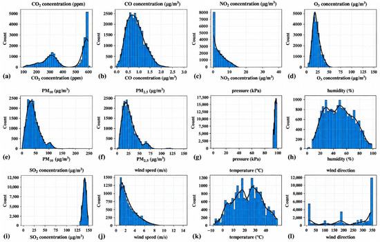
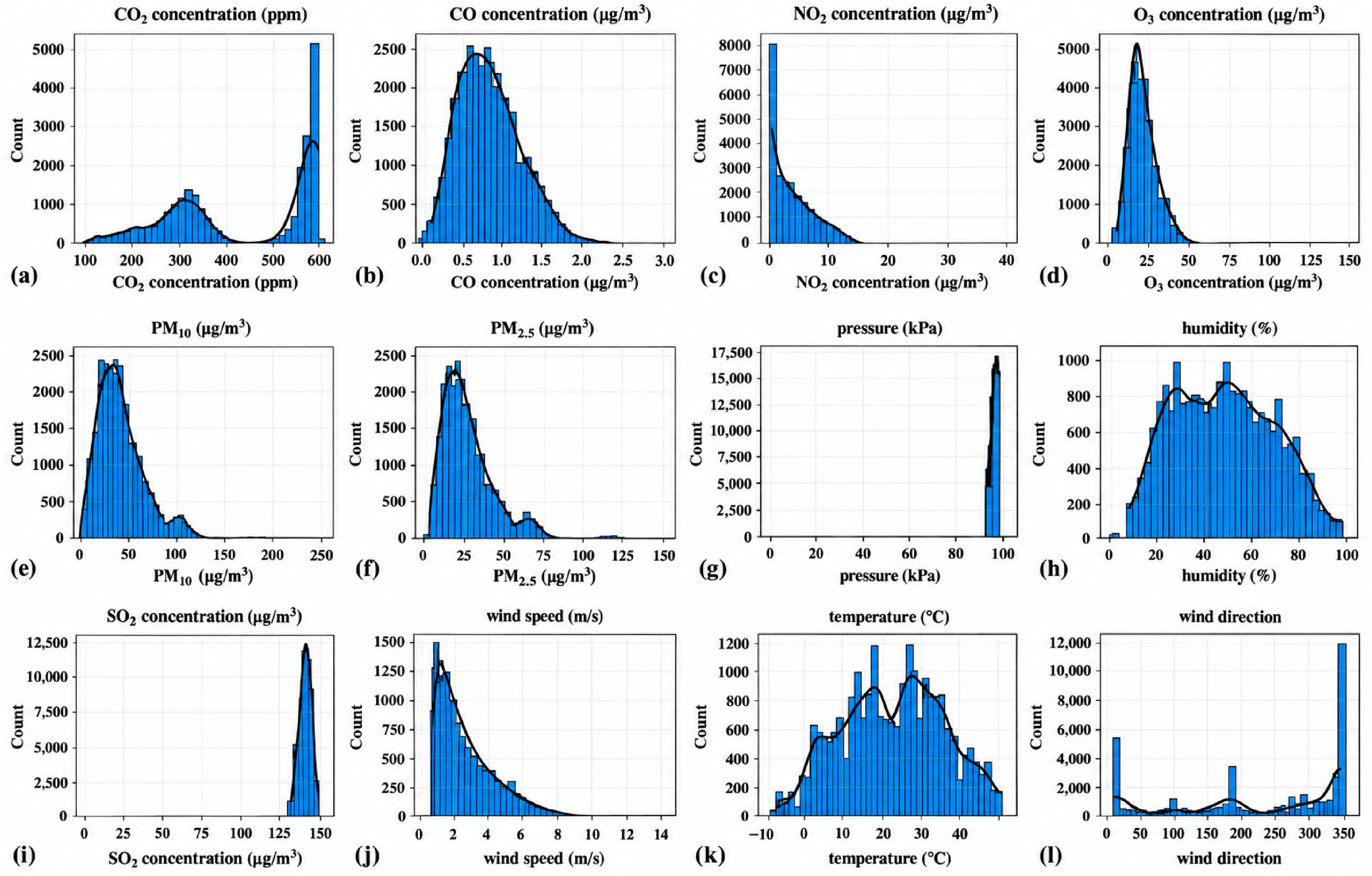
Beyond the numerical summary, the distributional structure of the quality-controlled dataset was further examined to evaluate the spread, central tendency, and variability of each variable. Therefore, the lidar-derived CO₂ concentration and environmental variables were visualized separately. As shown in Figure 3, the variables exhibit distinct distribution patterns, reflecting differences in pollutant concentration levels, meteorological conditions, and atmospheric transport characteristics during the observation period. This visualization complements Table 3 by showing the data distribution rather than only its summary statistics.

Figure 3. Distribution characteristics of lidar-derived CO₂ concentration and matched environmental variables after quality control. Multiple panels are listed as (a) CO₂-concentration distribution; (b) CO-concentration distribution; (c) NO₂-concentration distribution; (d) O₃-concentration distribution; (e) PM₁₀-concentration distribution; (f) PM_2.5-concentration distribution; (g) pressure distribution; (h) humidity distribution; (i) SO₂-concentration distribution; (j) wind-speed distribution; (k) temperature distribution; and (l) wind-direction distribution. Blue bars represent frequency, red curve represents KDE.

2.3. Analysis Method for Driving Factors of CO₂ Concentration

To analyze the influence of different environmental factors on the changes in CO₂ concentration, this study establishes an analysis framework that combines multiple model comparisons and cross-validation. This framework comprehensively employs physically inspired process models, data-driven models, and physics-guided neural-network models to depict the relationship between environmental factors and changes in CO₂ concentration from various perspectives, and it conducts a comprehensive assessment of driving factors based on the analysis results of each model.

2.3.1. Environmental Driving Factor-Analysis Model

Because the models differ in theoretical basis and calculation method, the environmental-driver analysis in this study included physically inspired process models, a data-driven model, a statistical time-lag method, and a physics-guided neural-network model. The physically inspired process models constructed features related to atmospheric transport and diffusion, the data-driven model extracted nonlinear relationships between environmental variables and CO₂ concentration, the statistical method analyzed time-lag response characteristics, and the physics-guided neural network improved prediction smoothness and physical consistency. Integrating these model outputs enabled a more comprehensive assessment of the drivers of CO₂-concentration variation.

• Physical-process model

(a)

PGT stability classification model

The Pasquill–Gifford–Turner (PGT) stability model is commonly used to classify the stability of the atmospheric boundary layer into six grades, A–F. Grades A–B correspond to relatively strong unstable conditions, while grades E–F represent stable stratification states. Under stable conditions, turbulent exchange weakens and the atmospheric vertical diffusion capacity decreases, which may lead to an increase in CO₂ concentration in the near-surface layer. Considering that the study area lacks complete input parameters, such as boundary layer height, surface heat flux, and temperature lapse rate, the code in this study adopts a simplified PGT stability proxy scheme. Based on diurnal conditions, solar angle proxy quantities, and wind speed, the stability numerical coding and diffusion capacity characteristics are constructed to represent the atmospheric stability state under different meteorological conditions.

Therefore, this study adopts a surrogate-model strategy. The surrogate model used simplified PGT stability coding, solar angle, diffusion capacity, and synchronized meteorological and pollutant variables as input features for a random forest (RF) regression model. Feature importance analysis then evaluated the influence of each environmental factor on CO₂ prediction.

The random-forest regressors use observed CO₂ concentration as the target and the environmental observations and derived proxy features as predictors. We summarize predictor importance using mean decrease in impurity (MDI), as returned by the fitted random-forest model.

For squared-error regression trees, a split reduces impurity when the parent-node mean squared error exceeds the sample-weighted mean squared errors of its children. The calculation weights this reduction by the fraction of training samples reaching the node and assigns it to the splitting feature. Normalization within each tree and averaging across trees produce the forest importance score. Only nodes that split on a given feature contribute to that feature’s score. MDI describes the fitted model and does not measure a causal contribution to atmospheric CO₂.

(b)

Gaussian plume diffusion model

The Gaussian plume diffusion model is based on mass-conservation and turbulent-diffusion theory. It assumes that pollutants follow a Gaussian distribution during transport and describes the spatial distribution of pollutant concentration under the influence of emission sources [33]. The model combines the Pasquill–Gifford–Turner (PGT) stability level to characterize atmospheric turbulence and determine the horizontal diffusion coefficient, σy, and vertical diffusion coefficient, σz.

The Gaussian plume diffusion model can describe the combined influence of emission intensity, wind field conditions, and the turbulent diffusion process on the spatial distribution of pollutants. However, in actual observations, emission parameters and local meteorological conditions are uncertain, and the output of the Gaussian formula is difficult to directly convert into a unified environmental-variable contribution index. Therefore, this study introduces a random-forest proxy model, combining Gaussian diffusion-related parameters with synchronous observed environmental variables, to construct an input feature set and predict CO₂ concentration.

In the code implementation of the attachment, the input features mainly include the horizontal diffusion parameter, σy; vertical diffusion parameter, σz; stability encoding; emission-intensity proxy quantity constructed from CO; and synchronous observed meteorological and pollutant variables. The calculated Gaussian concentration diagnostic quantity in the code is used to characterize the diffusion process, but it is not directly involved in the ranking of the importance of random forest features. The MDI index calculated by the random-forest regression model is used to evaluate the relative contribution of each input variable to the CO₂ prediction result.

(c)

Box model

The box-model component represents the atmospheric boundary layer as a well-mixed control volume [10]. In a conventional box model, changes in mean CO₂ concentration are described by a mass-balance relationship involving surface emissions, horizontal transport, vertical exchange, and boundary-layer entrainment. This framework provides a physical basis for regional-scale CO₂ simulation.

A complete CO₂ box model requires reliable emission fluxes, boundary-layer height, entrainment information, and transport parameters. These quantities cannot be fully constrained by the available observations. The implementation in this study does not directly solve the CO₂ mass-balance equation. The box-model concept is used to construct mixing- and transport-related predictors, which are combined with environmental observations in a random-forest model to reproduce observed CO₂-concentration variations.

The model inputs include observation time, solar angle, wind information, meteorological variables, pollutant concentrations, and derived diurnal and mixing-related features. Physically inspired parameterization refers here to empirical feature construction based on atmospheric mixing and transport concepts. Variables labelled in the archived code as boundary-layer height, mixing coefficient, and advection speed are proxy features estimated from available information such as time, solar angle, wind speed, and atmospheric stability. They are not direct observations or independently retrieved physical quantities.

The fitted random forest provides feature-importance scores for the input predictors. These scores are used to assess the relative contributions of environmental and mixing-related factors to observed CO₂ variability and to support physical interpretation within a box-model-inspired framework. They do not represent a direct quantitative decomposition of individual terms in the CO₂ mass-balance equation.

• Data-driven models

The XGBoost/Ensemble label denotes a weighted ensemble of random forest, gradient boosting, extra trees, ridge regression, support vector regression (SVR), and multilayer perceptron (MLP) predictions. The archived component uses fixed weights to combine these regressors; the label does not denote a single native XGBoost model.

To analyze the contribution of different environmental factors to the change in CO₂ concentration, this ensemble framework uses the feature importance of the random forest as the original indicator and attributes derived features such as wind vector, time period, interaction terms, pollutant aggregation terms, lag terms, and rolling statistics according to their physical meaning to the main environmental factors. This processing procedure differs from the Gain metric used in the native XGBoost model. Therefore, in this study, it is subsequently referred to as XGBoost/Ensemble feature importance or the result of feature attribution for the ensemble model.

During feature attribution, the model first obtains random-forest MDI importance values and then maps derived technical features back to the main environmental factors: CO, NO₂, O₃, PM₁₀, PM_2.5, SO₂, humidity, pressure, temperature, wind speed, and wind direction. This mapping provides a consistent basis for comparison with the environmental-contribution results from other models.

• Physical-Constraint Neural-Network Model

The PG-GRNN component adds a gradient penalty to neural-network regression to discourage rapid output changes with respect to its inputs. Physical information can enter neural models through different forms of constraints [34]. Here, the penalty expresses a smoothness assumption. It does not impose an atmospheric mass-balance equation or a transport-equation residual.

The training objective combines a mean squared error term with a weighted gradient penalty:

$$L_{total}=L_{data}+\lambda \cdot L_{reg}$$

(6)

The total objective combines the data-fitting loss and the gradient regularizer. The non-negative weight, λ, controls the strength of the penalty relative to data fitting. Smoothness alone does not establish physical consistency.

$L_{data}$ is the standard mean squared error (mean squared error, MSE):

$$L_{data}={\displaystyle \frac{1}{N}}{\displaystyle \sum _{i=1}^N}{(y}_i{-y_{{pred}_i})}^2$$

(7)

In Equation (7), $N$ is the number of training samples in the mean, i indexes those samples, $y_i$ is the standardized observed CO₂ value, and $y_{pred,i}$ is the standardized prediction. The gradient regularizer penalizes squared derivatives with respect to standardized input features.

Automatic differentiation computes these derivatives by applying the chain rule through the model’s computational graph. It provides the output gradients used in regularization and sensitivity calculations.

The environmental-variable sensitivity score, $S_j$, is the sample mean of the absolute derivative with respect to the j-th standardized input:

$$S_j={\displaystyle \frac{1}{N}}{\sum }_{i=1}^N\left|{\displaystyle \frac{\partial f_{\theta }\left(X_i\right)}{\partial X_{i,j}}}\right|$$

(8)

In Equation (8), i indexes samples, j indexes input features, and N is the number of samples in the average. $X_i$ is the standardized input vector of sample i, and $X_{i,j}$ is its j-th component. The function $f_{\theta }$ maps standardized inputs to the standardized model output, with $\theta$ denoting network parameters. $S_j$ measures model sensitivity in standardized coordinates; it does not measure a physical flux or causal effect. The absolute value prevents positive and negative gradients from cancelling.

• Time-lag analysis method

The Granger test evaluates whether past observations of an environmental variable improve prediction of CO₂ beyond the target’s own history. A lag-order $p$ includes the preceding 1 through p observations in the analysis sequence. Thus, order 2 includes both the first and second preceding observations. We compare orders 1–10 and identify the order with the smallest nominal p-value for each variable.

For each environmental predictor, the restricted regression includes an intercept and $p$ past CO₂ observations. The unrestricted regression adds $p$ past observations of that predictor. Both regressions use the same response records. The $F$ statistic compares their residual sums of squares:

$$F={\displaystyle \frac{\left(\mathrm{RS}{\mathrm{S}}_{\mathrm{r}}-\mathrm{RS}{\mathrm{S}}_{\mathrm{ur}}\right)/p}{\mathrm{RS}{\mathrm{S}}_{\mathrm{ur}}/\left(T-k\right)}}\sim F_{p,T-k}$$

(9)

In Equation (9), ${RSS}_r$ and ${RSS}_{ur}$ are the restricted and unrestricted residual sums of squares. The lag-order $p$ also gives the number of added predictor-history terms. $T$ is the number of usable regression rows after lag construction, and $k$ is the rank of the unrestricted design matrix, including the intercept. The denominator degrees of freedom are $T-k$. The test concerns the joint contribution of the added history terms. Reported p-values are nominal and unadjusted for comparisons across variables and lag orders.

2.3.2. Model Construction and Validation Methods

Based on the multi-source observational data that have undergone quality control and preprocessing, different models are constructed and validated. For data-driven models that require parameter fitting based on observational samples, a random partitioning method is used to divide the valid samples into training sets and test sets, where 80% of the samples are used for model construction, and 20% for independent validation. The random seed is set to 42 during the data partitioning process to ensure the reproducibility of the model calculation process and evaluation results.

The training samples are used to establish model parameter fitting and the response relationship between environmental factors and CO₂ concentration, and to optimize model parameters; the test samples are used to evaluate the model’s ability to simulate changes in CO₂ concentration. The model validation results are based on the deviation between the simulated values and the observed values, and include evaluation indicators such as the coefficient of determination (R²), mean squared error (MSE), and root mean squared error (RMSE).

2.3.3. Model Integration and Evaluation Methods

The analysis framework constructed in this study integrates physically inspired feature models, machine-learning models, and time-series analysis methods. By comparing and cross-validating different methods, the framework characterizes CO₂-concentration changes and their environmental drivers. The physically inspired models (PGT, Gaussian diffusion parameter model, and box mixing parameter model) construct input variables from atmospheric stability, pollutant diffusion, and regional mixing processes to represent mechanisms of CO₂ variability.

The data-driven model XGBoost/Ensemble analyzes the nonlinear mapping relationship between environmental variables and CO₂ concentration, and it evaluates the response characteristics in the high-dimensional environmental variable space based on the random-forest MDI proxy index and the physical-attribution process. The Granger time-lag predictability test analyzes the lag-response relationship between environmental variables and CO₂ concentration from the time-series perspective, and it evaluates the contribution of historical information of the variables to the prediction ability of CO₂ concentration. PG-GRNN introduces a gradient regularization term in the neural-network loss function to constrain the gradient response relationship between the network output and the input environmental variables, maintaining the prediction ability while improving the smoothness and physical consistency of the model prediction results.

The above six methods collectively form a multi-model collaborative analysis system. The results of different models can be used for mutual verification and to analyze the differences in the contribution characteristics of different methods to environmental factors. The comprehensive comparison of multi-model results can reduce the uncertainty caused by a single model analysis and improve the reliability of the analysis results.

The model evaluation system includes three aspects: prediction performance, variable contribution, and time lag. The model prediction performance is evaluated using the coefficient of determination (R²), mean squared error (MSE), and root mean squared error (RMSE); the variable contribution analysis evaluates different model features using the random forest mean decrease in impurity (MDI), XGBoost/Ensemble attribution importance, and PG-GRNN gradient sensitivity indicators; the time-lag feature is characterized by the significance level (p-value) and corresponding lag (lag) of the Granger test. The variable contribution results obtained from different models are normalized and can be used for comprehensive comparison of multi-model results.

2.3.4. Overall Flowchart

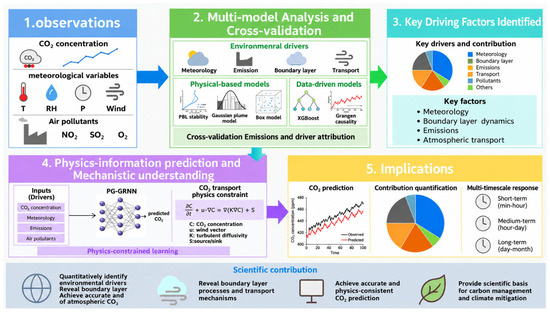
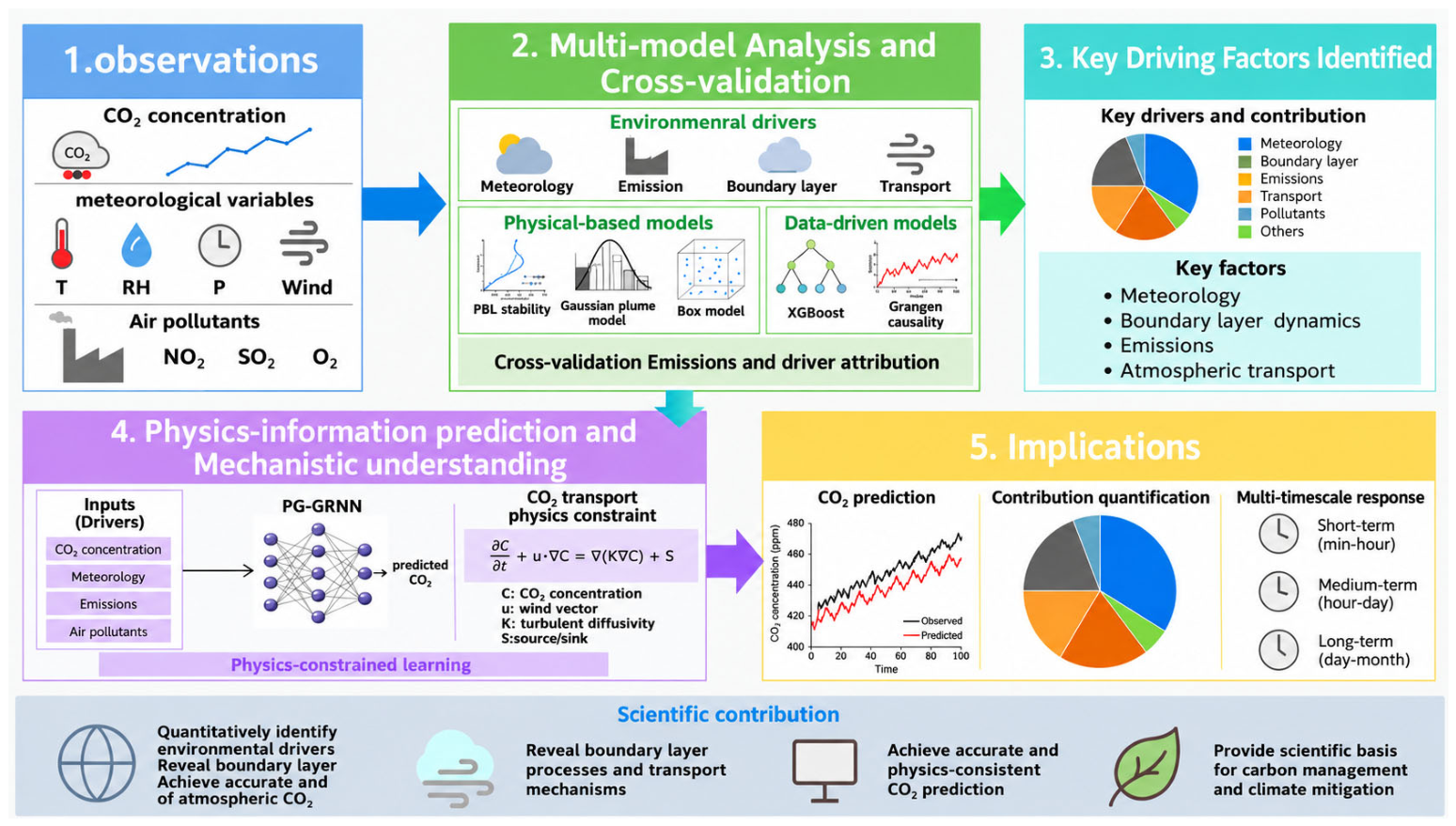
Figure 4 presents the workflow for analyzing CO₂ concentration with multi-source observations and environmental driving-factor models. The workflow links data acquisition, preprocessing, model analysis, result integration, and evaluation.

Figure 4. Workflow of the multi-model CO₂ analysis framework.

3. Results

3.1. Multi-Model Prediction Performance for CO₂ Concentration

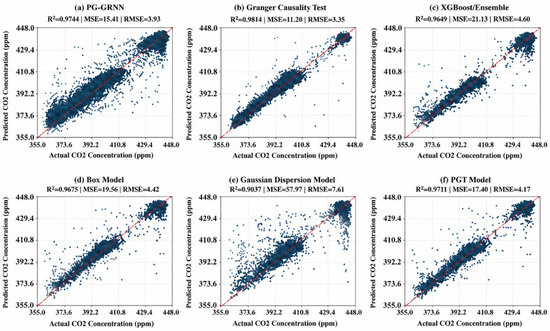
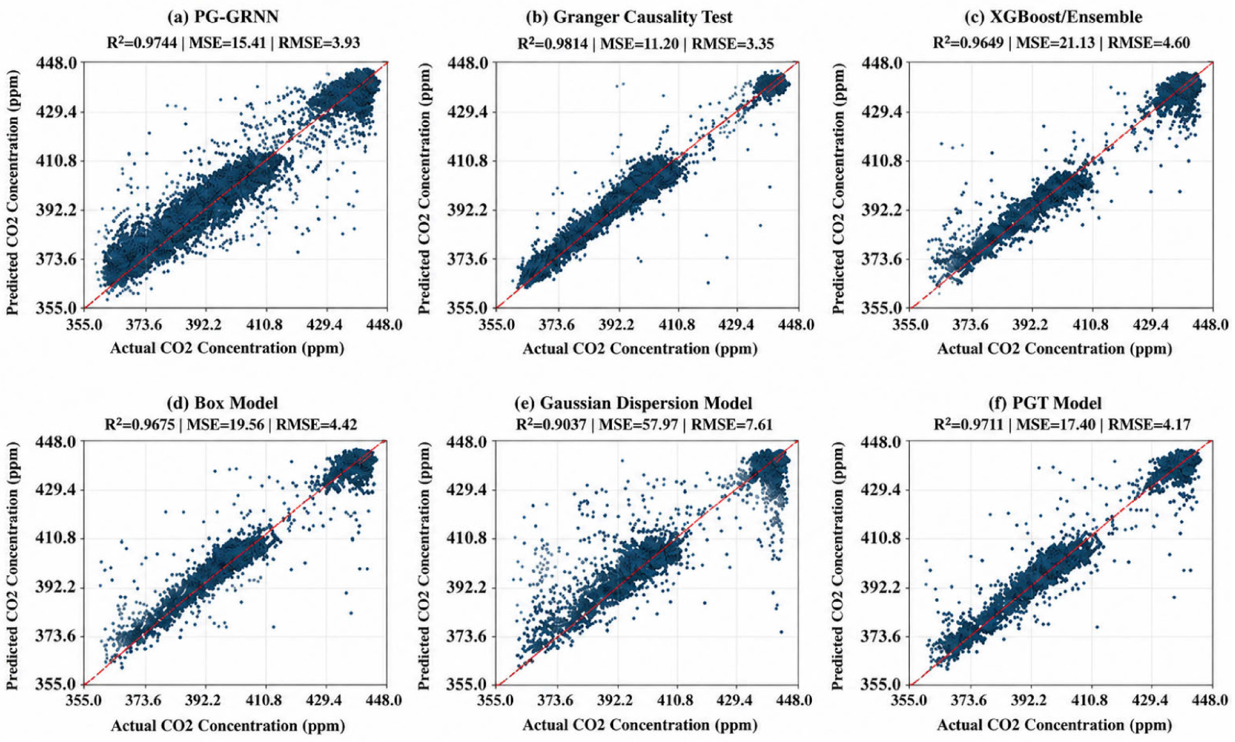
Figure 5 compares predicted and observed CO₂ concentrations for the six modelling and validation methods. All panels showed an overall alignment with the 1:1 reference line, indicating that the selected environmental variables captured the main variation in CO₂ concentration. The Granger-based panel gave the highest R² (0.9814), followed by the physics-guided neural-network/PG-GRNN panel (0.9744), PGT model (0.9711), box model (0.9675), and XGBoost/Ensemble model (0.9649). The Gaussian dispersion proxy model showed the lowest R² (0.9037) and greater scatter, especially at high CO₂ concentrations.

Figure 5. Multi-model prediction performance for CO₂ concentration, comparing predicted and observed CO₂ concentrations against the 1:1 reference line. Multiple panels are listed as (a) PG-GRNN model prediction performance; (b) Granger Causality Test prediction performance; (c) XGBoost/Ensemble model prediction performance; (d) box model prediction performance; (e) Gaussian Dispersion Model prediction performance; and (f) PGT Model prediction performance. Blue dots represent observed values, red line represents the 1:1 reference line.

These results indicate that no single model type fully dominated the prediction comparison. Temporal predictability and physics-guided learning produced the closest agreement with observations, whereas physically inspired diffusion and mixing proxies still reproduced the main concentration trend. The performance comparison therefore supports the use of a multi-model framework for subsequent driving-factor analysis rather than relying on a single model output.

3.2. Multi-Model Identification of Environmental Driving Factors

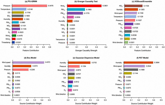
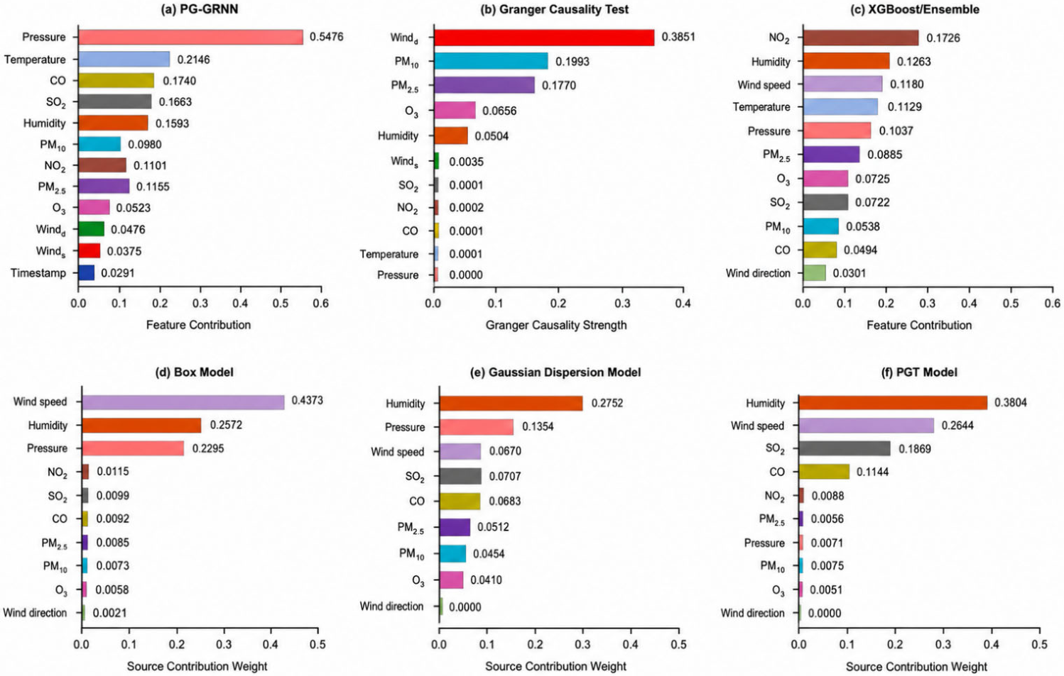
Figure 6 summarizes the method-specific rankings of environmental-variable contribution or predictive association. The leading variables differed among methods, showing that each model emphasized a different aspect of the CO₂ response. Pressure dominated the physics-guided neural-network/PG-GRNN sensitivity ranking (0.5476), whereas wind speed-related terms dominated the box model (0.4373) and the Granger-strength panel. Humidity ranked highest in the Gaussian dispersion and PGT proxy models, and NO₂ ranked highest in the XGBoost/Ensemble attribution result.

Figure 6. Method-specific rankings of environmental-variable contributions and predictive associations for CO₂ concentration. Multiple panels are listed as (a) feature-contribution ranking from the PG-GRNN model; (b) Granger causality strength ranking from the Granger Causality Test; (c) feature-contribution ranking from the XGBoost/Ensemble model; (d) source-contribution weight ranking from the box model; (e) source-contribution weight ranking from the Gaussian Dispersion Model; and (f) source-contribution weight ranking from the PGT Model.

The detailed rankings further show the complementary roles of meteorological and pollutant variables. In the PG-GRNN panel, pressure, temperature, CO, SO₂, and humidity were the leading contributors. In the Gaussian dispersion panel, humidity and pressure were the two largest contributors, followed by SO₂, CO, and wind speed. In the PGT panel, humidity, wind speed, SO₂, and CO were dominant, consistent with the role of stability and turbulent diffusion proxies.

After normalizing and integrating the method-specific outputs, the comprehensive importance sequence was pressure > temperature > humidity > NO₂ > SO₂ > CO > wind speed > PM_2.5 > PM₁₀ > O₃ > wind direction. This integrated result is consistent with the main result line of the manuscript: meteorological conditions provided the strongest background control on CO₂ variation, while combustion- and pollution-related variables, especially NO₂ and SO₂, supplied complementary information for short-timescale CO₂ changes. The disagreement among individual panels therefore reflects model perspective rather than a contradiction in the overall attribution result.

3.3. Time-Lag Influence of Environmental Factors

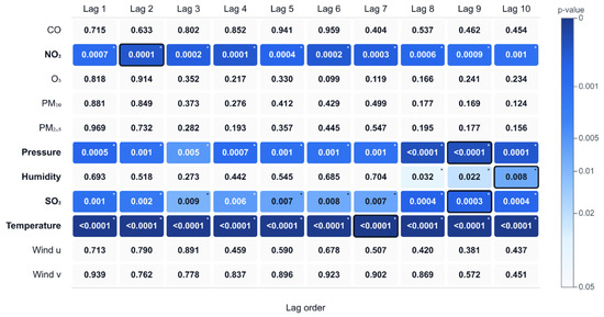
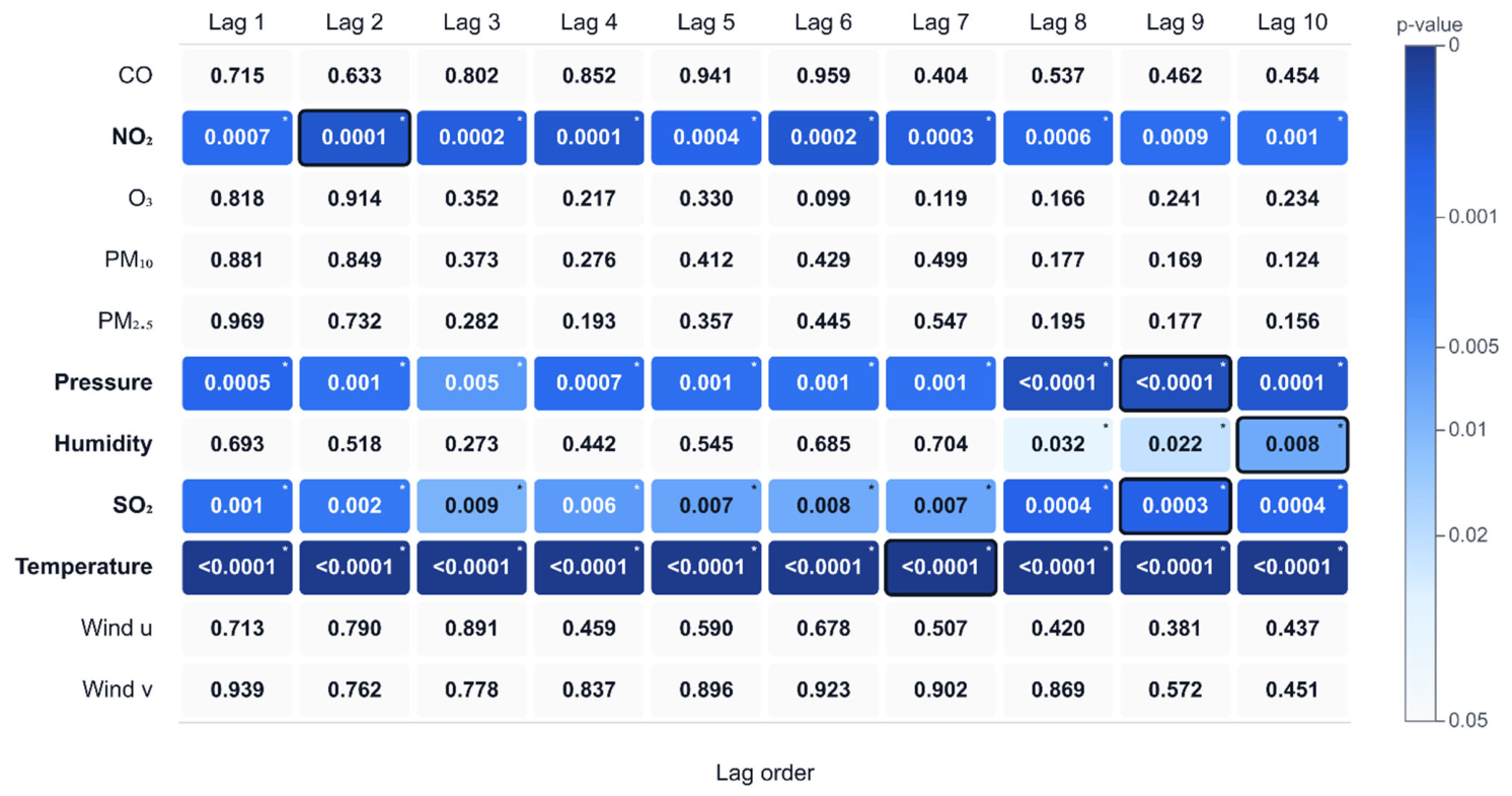
Granger time-predictability analysis identified lagged predictive relationships between environmental variables and CO₂ concentration. The analysis first-differenced the candidate variables to reduce non-stationary trends and then compared bivariate models across lag orders 1–10 (Figure 7). Historical information from NO₂, pressure, SO₂, temperature, and humidity significantly improved CO₂ prediction (p < 0.05), whereas CO, O₃, PM₁₀, PM_2.5, and wind components did not reach the significance threshold.

Figure 7. Lag-specific Granger time-predictability significance between environmental variables and CO₂ concentration. The color bar denotes the $p$-value of the Granger causality test. Black borders on blue blocks mark the optimal lag order corresponding to the minimum $p$-value for each variable. Asterisk symbols denote statistical significance at $p$ < 0.05.

In terms of optimal lag order, temperature showed the strongest significance at the 7th lag ($F$ = 8.99, $p$ = 4.02 × 10⁻¹¹), while the optimal lag for NO₂ was 2 ($F$ = 8.95, $p$ = 1.30 × 10⁻⁴), indicating that thermal conditions and combustion-emission-related variables provided stronger predictive information at moderate and short lag scales, respectively. The optimal lags for pressure and SO₂ were both 9 ($F$ = 3.89, $p$ = 6.02 × 10⁻⁵; $F$ = 3.42, $p$ = 3.26 × 10⁻⁴), and the optimal lag for humidity was 10 ($F$ = 2.39, $p$ = 7.80 × 10⁻³). This pattern suggests that meteorological conditions and some pollutant variables contain longer-lag predictive information for CO₂ variation.

These results indicate clear differences in lag-prediction structures among environmental variables: NO₂ provided short-lag predictive information; temperature showed the strongest signal at a moderate lag; and pressure, SO₂, and humidity retained significant predictive information at longer lag scales. Because the Granger test measures the gain from historical information in prediction accuracy, these results should be interpreted as time-predictable relationships rather than strict physical causal relationships.

4. Discussion

4.1. Interpretation of the Multi-Model Results

Pressure, temperature, humidity, NO₂, and SO₂ were the most consistent environmental factors associated with regional CO₂ variation across the multi-model results. Meteorological factors had the highest integrated importance, indicating that boundary-layer structure, atmospheric stability, and diffusion conditions governed CO₂ accumulation and dilution. Pressure contributed most strongly in the PG-GRNN sensitivity result, probably because it reflects regional atmospheric state and boundary-layer diffusion conditions. Temperature and humidity further regulate CO₂ variation through atmospheric thermodynamic structure, turbulent exchange, and ecosystem carbon exchange.

Among the pollutant variables, NO₂ showed high importance in multiple models and significant short-term lagged predictive information in the Granger test. CO can serve as a tracer of incomplete-combustion emissions and contributed in some feature-importance results, but it did not reach the significance threshold in the Granger test, indicating that its relationship with CO₂ more likely reflects synchronous emissions or common-source associations than stable lagged predictive effects. The Granger analysis further showed that NO₂, temperature, pressure, SO₂, and humidity had predictive correlations with CO₂ concentration at different timescales, indicating that the influence of environmental factors on CO₂ variation was not completely synchronous.

The six-method comparison clarifies why a single attribution method is insufficient. Pressure and humidity dominated the physics-guided and physically inspired panels, NO₂ dominated the XGBoost/Ensemble attribution, and the Granger test identified NO₂ as the shortest-lag predictive pollutant. These differences support the integrated ranking reported in Section 3.2 because each method captures a different part of the CO₂–environment relationship.

PG-GRNN achieved high fitting accuracy in CO₂-concentration prediction (R² = 0.9744; MSE = 15.41). Gradient regularization constrained the response between network output and environmental inputs, improving prediction smoothness and physical consistency in the data-driven model.

The time-series predictability analysis revealed lagged predictive relationships between environmental variables and CO₂ concentration. The Granger test showed that NO₂, pressure, SO₂, temperature, and humidity had significant lagged predictive correlations with CO₂ variation, while CO, O₃, PM₁₀, PM_2.5, and wind-speed components did not reach the significance threshold. The optimal lag of NO₂ was second-order, reflecting the contribution of short-term pollution-emission information to CO₂ prediction; temperature had the highest significance at the seventh lag, the optimal lags of pressure and SO₂ were both ninth-order, and the optimal lag of humidity was 10th-order, indicating that CO₂ variation was influenced by short-lag emission associations, medium-lag thermodynamic conditions, and longer-lag meteorological states. These results show clear timescale differences among environmental variables in relation to CO₂ variation.

The multi-model framework combines data-driven prediction, physically inspired attribution, physics-guided regularization, and time-series testing. It supports environmental-driver analysis for CO₂ concentration and provides a basis for ground-based and remote-sensing CO₂ data fusion.

4.2. Spatial Transferability and Practical Applications

The prominence of meteorological variables in Nanyang suggests that mixing-related factors may provide useful candidate predictors at sites with similar climatic conditions. However, factor rankings and lag orders are expected to vary with local emission sources, ecosystem characteristics, and transport processes. Temperature and humidity may be more informative in regions dominated by biogenic exchange, whereas NO₂ may be more relevant in urban areas with strong combustion emissions. Wind-related variables may become more important in coastal regions. Therefore, transferring the framework to another site requires local data preprocessing, model calibration, and independent validation.

The framework can support variable selection and monitoring-system design where synchronized CO₂, meteorological, and air-quality observations are available. Locally validated rankings may help determine sensor-accuracy and maintenance priorities. Lagged variables may also serve as candidate predictors for future short-term CO₂ forecasting and warning systems, although forecasting performance was not evaluated in this study. The present findings are limited to one site, a 38-day observation period, and a CO₂-averaging layer of 210–600 m.

5. Conclusions

This study focused on continuous CO₂ observations from ground-based hyperspectral Raman lidar and developed an environmental-factor analysis framework integrating physically inspired features, ensemble machine learning, PG-GRNN, and Granger time-predictability testing. The vertically averaged CO₂ concentration within 210–600 m was used as the target variable to evaluate the explanatory contribution and predictive information of meteorological factors and pollutant concentrations during the observation period.

The multi-model results indicate that pressure, temperature, humidity, NO₂, and SO₂ were the environmental factors most consistently associated with CO₂ variations during the observation period. The overall importance ranking was pressure > temperature > humidity > NO₂ > SO₂ > CO > wind speed > PM_2.5 > PM₁₀ > O₃ > wind direction. This pattern suggests that near-surface CO₂ variations were affected by combustion-related pollutant signals and were closely related to boundary-layer thermal conditions, diffusion capacity, and atmospheric stability. Pressure and temperature ranked highest in the integrated importance assessment, indicating the role of meteorological conditions in constraining CO₂ accumulation, dilution, and vertical mixing. NO₂ maintained relatively high contributions across multiple models, suggesting that combustion-related signals provide useful information for short-timescale CO₂ variations.

PG-GRNN achieved high fitting accuracy under the current data partition, with an R² of 0.9744 and an MSE of 15.41. The gradient regularization constraint allowed the model to capture nonlinear response relationships while maintaining smooth output variation. This result supports physics-guided neural networks for stable CO₂ simulation, while the full multi-model comparison remains necessary to separate model-specific sensitivity from cross-method attribution.

Granger time-predictability analysis further characterized the lag structure between environmental factors and CO₂ variations. The optimal lag order was 2 for NO₂, 7 for temperature, 9 for both pressure and SO₂, and 10 for humidity. CO, O₃, PM₁₀, PM_2.5, and wind components did not show stable lagged predictability at the p < 0.05 level. This lag pattern suggests that CO₂ variations contain short-lag emission-related information, medium-lag thermal regulation, and longer-lag meteorological-state information. The Granger test quantifies the predictive gain provided by historical variables for CO₂ prediction; therefore, these results should be interpreted as time-predictable relationships rather than direct physical causality.

The results provide a reference for ground-based CO₂ data fusion, validation of lidar and remote-sensing CO₂ products, and analysis of regional carbon-concentration responses to environmental conditions. Given the limitations of the observation period and single-station data, future studies should incorporate longer time series, multi-site observations, boundary-layer height, flux measurements, and emission inventories to further evaluate the stability and spatial applicability of the identified key environmental factors.

References

- Eyring, V.; Collins, W.D.; Gentine, P.; Barnes, E.A.; Barreiro, M.; Beucler, T.; Bocquet, M.; Bretherton, C.S.; Christensen, H.M.; Dagon, K.; et al. Pushing the frontiers in climate modelling and analysis with machine learning. Nat. Clim. Change 2024, 14, 916–928. [Google Scholar] [CrossRef] [Scilit]
- Han, G.; Zhang, H.; Huang, Y.; Chen, W.; Mao, H.; Zhang, X.; Ma, X.; Li, S.; Zhang, H.; Liu, J.; et al. First global XCO2 observations from spaceborne lidar: Methodology and initial result. Remote Sens. Environ. 2025, 330, 114954. [Google Scholar] [CrossRef] [Scilit]
- Han, G.; Huang, Y.; Shi, T.; Zhang, H.; Li, S.; Zhang, H.; Chen, W.; Liu, J.; Gong, W. Quantifying CO2 emissions of power plants with Aerosols and Carbon Dioxide Lidar onboard DQ-1. Remote Sens. Environ. 2024, 313, 114368. [Google Scholar] [CrossRef] [Scilit]
- Han, G.; Wang, H.; Pei, Z.; Mao, H.; Ying, J.; Li, S.; Ma, X.; Liu, B.; Mao, F.; Gong, W. Quantifying facility-scale CO2 emissions using spaceborne hyperspectral imageries. Remote Sens. Environ. 2026, 342, 115478. [Google Scholar] [CrossRef] [Scilit]
- Zhang, Y.; Han, G.; Huang, Y.; Wang, H.; Zhang, H.; Pei, Z.; Pu, Y.; Luo, H.; Yi, J.; Shi, T.; et al. Attributing GHG emissions to individual facilities using multi-temporal hyperspectral images: Methodology and applications. ISPRS J. Photogramm. Remote Sens. 2026, 232, 937–956. [Google Scholar] [CrossRef] [Scilit]
- Gifford, F.A.; Hanna, S.R. Modelling urban air pollution. Atmos. Environ. 1973, 7, 131–136. [Google Scholar] [CrossRef] [Scilit] [PubMed]
- Hu, S.; Jia, X.; Zhang, J.; Kong, W.; Cao, Y. Shortcomings/Limitations of Blockwise Granger Causality and Advances of Blockwise New Causality. IEEE Trans. Neural Netw. Learn. Syst. 2016, 27, 2588–2601. [Google Scholar] [CrossRef] [Scilit] [PubMed]
- Kahl, J.D.W.; Chapman, H.L. Atmospheric stability characterization using the Pasquill method: A critical evaluation. Atmos. Environ. 2018, 187, 196–209. [Google Scholar] [CrossRef] [Scilit]
- Mohan, M.; Siddiqui, T.A. Analysis of various schemes for the estimation of atmospheric stability classification. Atmos. Environ. 1998, 32, 3775–3781. [Google Scholar] [CrossRef] [Scilit]
- Ragland, K.W. Multiple box model for dispersion of air pollutants from area sources. Atmos. Environ. 1973, 7, 1017–1032. [Google Scholar] [CrossRef] [Scilit]
- Venkatram, A. An examination of the Pasquill-Gifford-Turner dispersion scheme. Atmos. Environ. 1996, 30, 1283–1290. [Google Scholar] [CrossRef] [Scilit]
- Amarpuri, L.; Yadav, N.; Kumar, G.; Agrawal, S. Prediction of CO2 emissions using deep learning hybrid approach: A Case Study in Indian Context. In Proceedings of the 2019 Twelfth International Conference on Contemporary Computing (IC3), Noida, India, 8–10 August 2019; pp. 1–6. [Google Scholar] [CrossRef] [Scilit]
- Begum, A.M.; Mobin, M.A. A machine learning approach to carbon emissions prediction of the top eleven emitters by 2030 and their prospects for meeting Paris agreement targets. Sci. Rep. 2025, 15, 19469. [Google Scholar] [CrossRef] [Scilit] [PubMed]
- Desdhanty, V.S.; Rustam, Z. Liver Cancer Classification Using Random Forest and Extreme Gradient Boosting (XGBoost) with Genetic Algorithm as Feature Selection. In Proceedings of the 2021 International Conference on Decision Aid Sciences and Application (DASA) Sakheer, Sakheer, Bahrain, 7–8 December 2021; pp. 716–719. [Google Scholar] [CrossRef] [Scilit]
- Frifra, A.; Maanan, M.; Maanan, M.; Rhinane, H. Harnessing LSTM and XGBoost algorithms for storm prediction. Sci. Rep. 2024, 14, 11381. [Google Scholar] [CrossRef] [Scilit] [PubMed]
- Ji, Z.; Song, H.; Lei, L.; Sheng, M.; Guo, K.; Zhang, S. A Novel Approach for Predicting Anthropogenic CO2 Emissions Using Machine Learning Based on Clustering of the CO2 Concentration. Atmosphere 2024, 15, 323. [Google Scholar] [CrossRef] [Scilit]
- Kadam, P.; Vijayumar, S. Prediction Model: CO2 Emission Using Machine Learning. In Proceedings of the 2018 3rd International Conference for Convergence in Technology (I2CT), Pune, India, 6–8 April 2018; pp. 1–3. [Google Scholar] [CrossRef] [Scilit]
- Khorram, M.; Faria, P.; Abrishambaf, O.; Vale, Z.; Soares, J. CO2 Concentration Forecasting in an Office Using Artificial Neural Network. In Proceedings of the 2019 20th International Conference on Intelligent System Application to Power Systems (ISAP), New Delhi, India, 10–14 December 2019; pp. 1–6. [Google Scholar] [CrossRef] [Scilit]
- Kowsigan, M.; Shetty, R.; Vyas, A. Machine Learning-Based CO2 Emission Forecasting: A Predictive Modeling Approach for Sustainable Development. In Proceedings of the 2024 IEEE International Conference on Smart Power Control and Renewable Energy (ICSPCRE), Rourkela, India, 19–21 July 2024; pp. 1–6. [Google Scholar] [CrossRef] [Scilit]
- Mardani, A.; Liao, H.; Nilashi, M.; Alrasheedi, M.; Cavallaro, F.A.; Abbaszadeh, M.A. A multi-stage method to predict carbon dioxide emissions using dimensionality reduction, clustering, and machine learning techniques. J. Clean. Prod. 2020, 275, 122942. [Google Scholar] [CrossRef] [Scilit]
- Shao, Q.; Chen, J.; Jiang, T. A Novel Coupled Optimization Prediction Model for Air Quality. IEEE Access 2023, 11, 69667–69685. [Google Scholar] [CrossRef] [Scilit]
- Farea, A.; Yli-Harja, O.; Emmert-Streib, F. Understanding Physics-Informed Neural Networks: Techniques, Applications, Trends, and Challenges. AI 2024, 5, 1534–1557. [Google Scholar] [CrossRef] [Scilit]
- Faroughi, S.A.; Pawar, N.M.; Fernandes, C.; Raissi, M.; Das, S.; Kalantari, N.K.; Kourosh Mahjour, S. Physics-Guided, Physics-Informed, and Physics-Encoded Neural Networks and Operators in Scientific Computing: Fluid and Solid Mechanics. J. Comput. Inf. Sci. Eng. 2024, 24, 040802. [Google Scholar] [CrossRef] [Scilit]
- Karniadakis, G.E.; Kevrekidis, I.G.; Lu, L.; Perdikaris, P.; Wang, S.; Yang, L. Physics-informed machine learning. Nat. Rev. Phys. 2021, 3, 422–440. [Google Scholar] [CrossRef] [Scilit]
- Raissi, M.; Perdikaris, P.; Karniadakis, G.E. Physics-informed neural networks: A deep learning framework for solving forward and inverse problems involving nonlinear partial differential equations. J. Comput. Phys. 2019, 378, 686–707. [Google Scholar] [CrossRef] [Scilit]
- Shokouhi, P.; Kumar, V.; Prathipati, S.; Hosseini, S.A.; Giles, C.L.; Kifer, D. Physics-informed deep learning for prediction of CO2 storage site response. J. Contam. Hydrol. 2021, 241, 103835. [Google Scholar] [CrossRef] [Scilit] [PubMed]
- Zhao, C.; Zhang, F.; Lou, W.; Wang, X.; Yang, J. A comprehensive review of advances in physics-informed neural networks and their applications in complex fluid dynamics. Phys. Fluids 2024, 36, 101301. [Google Scholar] [CrossRef] [Scilit]
- Zucker, S.; Batenkov, D.; Segal Rozenhaimer, M. Physics-informed neural networks for modeling atmospheric radiative transfer. J. Quant. Spectrosc. Radiat. Transf. 2025, 331, 109253. [Google Scholar] [CrossRef] [Scilit]
- Her, Y.; Yoo, S.-H.; Cho, J.; Hwang, S.; Jeong, J. Uncertainty in hydrological analysis of climate change: Multi-parameter vs. multi-GCM ensemble predictions. Sci. Rep. 2019, 9, 4974. [Google Scholar] [CrossRef] [Scilit] [PubMed]
- Yuval, J.; O’Gorman, P.A. Stable machine-learning parameterization of subgrid processes for climate modeling at a range of resolutions. Nat. Commun. 2020, 11, 3295. [Google Scholar] [CrossRef] [Scilit] [PubMed]
- Jing, Y.; Shi, J.; Wang, T. Evaluation and comparison of atmospheric CO2 concentrations from models and satellite retrievals. In Proceedings of the 2015 IEEE International Geoscience and Remote Sensing Symposium (IGARSS), Milano, Italy, 26–31 July 2015; pp. 2202–2205. [Google Scholar] [CrossRef] [Scilit]
- Zhang, M.; Li, X.; Wang, L. An Adaptive Outlier Detection and Processing Approach Towards Time Series Sensor Data. IEEE Access 2019, 7, 175192–175212. [Google Scholar] [CrossRef] [Scilit]
- Polat, H.M.; Coelho, F.M.; Vlugt, T.J.H.; Franco, F.M.; Tsimpanogiannis, I.N.; Moultos, O.A. Diffusivity of CO2 in H2O: A Review of Experimental Studies and Molecular Simulations in the Bulk and in Confinement. J. Chem. Eng. Data 2024, 69, 3296–3329. [Google Scholar] [CrossRef] [Scilit] [PubMed]
- Shen, S.; Li, L.; Gao, S.; Wang, Y.; Gu, L.; Li, S.; Zhu, X.; Jiang, J.; Yu, J.; Ren, W. High Resolution Diffuse Optical Tomography via Neural Fields. IEEE Trans. Comput. Imaging 2025, 11, 955–966. [Google Scholar] [CrossRef] [Scilit]
Disclaimer/Publisher’s Note: The statements, opinions and data contained in all publications are solely those of the individual author(s) and contributor(s) and not of MDPI and/or the editor(s). MDPI and/or the editor(s) disclaim responsibility for any injury to people or property resulting from any ideas, methods, instructions or products referred to in the content. |
© 2026 by the authors. Licensee MDPI, Basel, Switzerland. This article is an open access article distributed under the terms and conditions of the Creative Commons Attribution (CC BY) license.