


Abstract
Deciduous dipterocarp forests (DDFs), widespread in mainland Southeast Asia, are potentially important yet poorly quantified sources of isoprene, a dominant biogenic VOC and ozone/aerosol precursor, and observation-based estimates are essentially absent for DDFs in northern Thailand. We present a pilot study estimating canopy isoprene over a DDF at the University of Phayao using a zero-dimensional (0-D) Guenther (G93) box model, benchmarked against tree-based machine learning (ML). Modeled concentrations were compared with 30 wet-season tower samples (parts per trillion; thermal-desorption GC–MS) at three heights (12, 27, and 42 m) over four days. An effective mixing height was calibrated per level and evaluated by strict leave-one-day-out cross-validation. The model reproduced the mean daytime level and diurnal accumulation shape (cross-validated R2 = 0.64–0.68; MAPE ≈ 11%); because the clear-sky forcing is near-invariant, this reflects the within-day signal rather than day-to-day skill. A sensitivity analysis showed that the emission factor, loss rate, and mixing height are confounded through the ratio Es/(kH). In this exploratory comparison, supplying the box-model output as an ML feature recovered skill otherwise lost (ΔR2 up to +1.16), but an hour-of-day feature did the same, so the box model matches a diurnal-climatology baseline and its advantage is interpretability. This exploratory workflow offers a simple, low-data approach for tropical BVOC estimation.
1. Introduction
Isoprene (2-methyl-1,3-butadiene, C5H8) is the single most abundant biogenic volatile organic compound (BVOC) emitted to the atmosphere, with global emissions estimated at 440–600 Tg C yr−1 [1]. Because it reacts rapidly with the hydroxyl radical (OH), isoprene strongly influences the oxidative capacity of the troposphere, tropospheric ozone formation, and secondary organic aerosol (SOA) production [2,3]. It is produced in chloroplasts via the methylerythritol-phosphate (MEP) pathway and emitted in a light- and temperature-dependent manner, primarily during daytime [2,4]. Emission is highly species-specific and spatially and temporally variable, controlled chiefly by photosynthetically active radiation (PAR) and leaf temperature [5,6].
Tropical forests dominate the global isoprene source, and within mainland Southeast Asia the deciduous dipterocarp forest (DDF) is one of the most extensive natural vegetation types, occurring widely across northern and northeastern Thailand on shallow, often gravelly soils at roughly 300–900 m elevation [6]. A DDF is strongly seasonal, and its isoprene-emitting potential varies accordingly: dry-season leaf shedding and a water-stress response reduces the potential to a minimum, whereas leaf flush and high photosynthetic activity before and at the onset of the rainy season drive it to its seasonal peak [2]. Its canopy is dominated by members of the family Dipterocarpaceae (e.g., Shorea and Dipterocarpus spp.), although these dominant dipterocarps are generally weak isoprene emitters; the co-occurring oaks (Quercus spp.) are typically strong emitters, and an above-canopy isoprene flux has been reported over such forests [7]. A minor floristic component can therefore make a DDF a potentially important but largely unquantified regional BVOC source. This is particularly relevant for northern Thailand, where recurrent dry-season ozone and particulate episodes raise the question of how much biogenic isoprene contributes to regional photochemistry alongside biomass-burning and anthropogenic emissions [8].
Despite this potential importance, the observational and modeling basis for biogenic emissions in Thailand—and in mainland Southeast Asia more broadly—remains limited. Regional isoprene research has concentrated on equatorial evergreen rainforests, where canopy-scale fluxes and ambient concentrations have been characterized in dedicated field campaigns [7], whereas the seasonally deciduous DDF that dominates the continental interior has received far less attention. Within Thailand, air-quality research has focused predominantly on anthropogenic VOCs and on biomass-burning emissions associated with the recurrent dry-season haze of the north, while the biogenic contribution is typically represented through global, land-cover-based inventories such as MEGAN, using default plant-functional-type emission factors and generic phenology [1,8]. Because canopy- and leaf-level emission measurements for Thai dipterocarp species are scarce, these inventories carry large, mostly unquantified uncertainty for DDF, particularly given the pronounced seasonal leaf dynamics that modulate emission capacity. Mechanistic, observation-constrained estimates at the site level are therefore needed but remain essentially absent for this forest type. The flux tower at the University of Phayao (DPT site), established within a representative DDF stand in northern Thailand and instrumented for micrometeorological and concentration measurements (Section 2), offers a rare opportunity to develop and test such an estimate.
Process-based emission algorithms—beginning with the empirical light and temperature activity factors of Guenther et al. [5] (hereafter G93) and later generalized in the MEGAN framework [1]—remain the workhorse for biogenic emission estimation. Coupled with a simple mass balance, a zero-dimensional (0-D) box model can translate emission fluxes into ambient concentrations [9]. Such reduced-complexity models are interpretable and require few inputs, making them attractive in data-poor settings, but their parameters (emission factors, chemical lifetimes, and mixing depths) are uncertain and only partly identifiable—an issue rarely examined explicitly. In parallel, machine learning (ML) is increasingly applied to atmospheric and ecosystem fluxes [10]; purely data-driven models capture nonlinear relationships but may overfit, extrapolate poorly with small datasets, and lack physical interpretability. Physics-informed (hybrid) approaches, in which outputs or constraints from a process model are supplied to an ML model, aim to combine the strengths of both [10,11], yet whether such hybridization adds value for BVOC estimation in a genuinely data-limited tropical setting remains untested.
Addressing these gaps, the present study provides an observation-constrained box-model estimate of isoprene for a tropical DDF; it further diagnoses the structural identifiability of the model parameters and benchmarks the physical model against tree-based ML using the box-model output itself as a physics-informed feature. Accordingly, the main objective is to develop and rigorously cross-validate a simplified, interpretable box-model estimate of canopy isoprene over a DDF in northern Thailand and to assess whether coupling it with machine learning improves data-driven prediction. Because only four sampling days are available, the work is framed explicitly as a pilot study, adopting conservative, regularized ML with explicit overfitting diagnostics.
2. Materials and Methods
The overall study workflow is summarized in Figure 1. Two shared inputs, meteorological drivers (PAR from solar geometry over 08:00–18:00 LT and leaf temperature) and tower observations of canopy isoprene at 12, 27, and 42 m (active pumped sampling, TD–GC–MS), feed two parallel tracks. In the physics track, the drivers force the G93 emission algorithm within a 0-D box model; the model is calibrated via a per-level effective mixing height, evaluated by leave-one-day-out cross-validation, and probed by a sensitivity analysis of k and Es. In the data-driven track, regularized tree-based models (Random Forest and XGBoost) are trained under the same cross-validation, comparing Pure-ML features against a physics-informed hybrid that adds the box-model output. The two tracks converge in a three-way comparison of Pure Physics, Pure ML, and the hybrid.
2.1. Study Site and Vegetation
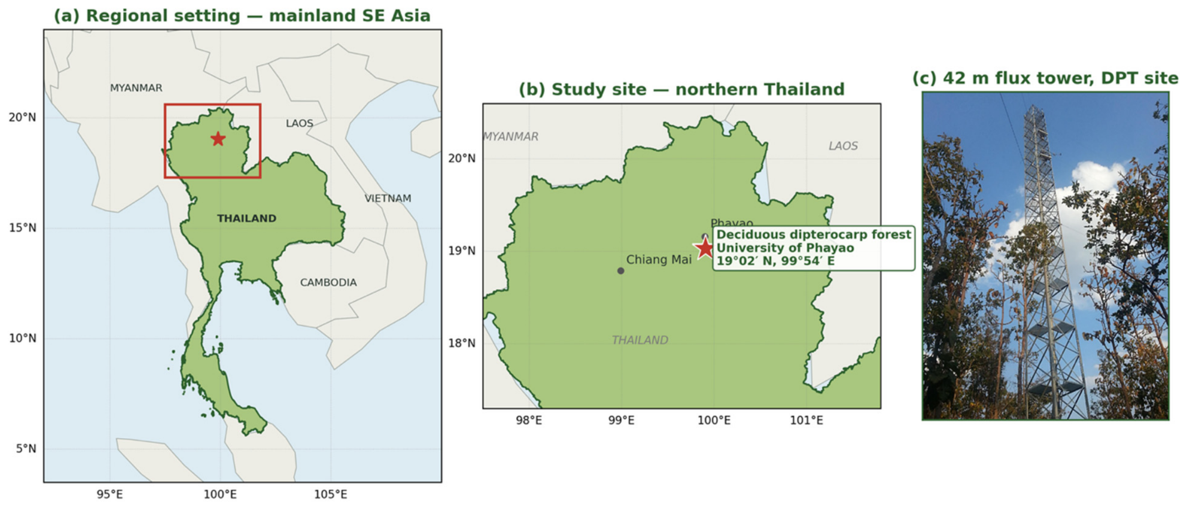
Measurements were made at the Dry Dipterocarp Forest Flux Phayao site (DPT), a ThaiFlux/AsiaFlux network site established in 2013 under the JST–JICA IMPAC-T project on the University of Phayao campus, Doi Luang Mountain, northern Thailand (19°02′14.4″ N, 99°54′11.0″ E; 512 m a.s.l.) [12]. The site is a deciduous (dry) dipterocarp forest—the most widespread seasonally dry forest type in mainland Southeast Asia—with an open, relatively low and structurally heterogeneous canopy dominated by light-demanding dipterocarps such as Shorea obtusa, Shorea siamensis, and Dipterocarpus tuberculatus, together with co-occurring oaks (Quercus spp.) [13]. Although the dominant dipterocarps are generally weak isoprene emitters, the co-occurring oaks (Quercus spp.) are typically strong emitters and are the more likely isoprene source at this site; canopy isoprene emission is thus strongly species-specific [14]. The substantial canopy-level isoprene observed here therefore illustrates that a minor floristic component can dominate ecosystem-scale isoprene emission—one motivation for quantifying concentrations at the ecosystem level rather than inferring them from the dominant taxa. The early–wet-season campaign analyzed here (late June–early July) coincides with fully developed, photosynthetically active foliage—conditions that favor high light- and temperature-dependent isoprene emission [5]. The stand has an average canopy height of about 16 m and a density of ~2150 trees ha−1 [12]; it is a young secondary forest that regenerated after past forestry concessions, with tree ages of 15–20 years as of 2015 [15]. It lies on sloping terrain with poor laterite soils within the Ing River watershed, a tributary of the Mekong, and experiences a tropical monsoon climate with a mean annual precipitation of 1262 mm (1998–2007, the period reported in the site description [12]); more recent on-site records at the DPT station (2013–2016) indicate a lower total of ~936 mm yr−1 [15], reflecting both the different reference period and measurement source and mean annual minimum and maximum air temperatures of 16.9 °C and 35.7 °C, respectively [12]. The trees shed their leaves, and the stand becomes largely bare in the dry season, when near-annual surface fires occur between November and March, with leaf flush following the first rains in late March–April [12]. A 42 m micrometeorological tower at the site supports eddy-covariance and routine meteorological measurements, including air temperature, humidity, and precipitation at 36 m [12]. The isoprene air-sampling ports analyzed here (12, 27, and 42 m) are mounted on this tower and span the canopy from below to well above it; the below-, at-, and above-canopy designations of the three levels follow this fixed-port configuration (Figure 2).
Figure 1.
Study workflow: meteorological drivers and tower observations feed a physics-based box model (G93 emission and 0-D mass balance); the model is calibrated (effective mixing height) and evaluated by leave-one-day-out cross-validation and sensitivity analysis. In parallel, a machine-learning pilot (Random Forest/XGBoost) uses the same drivers, with the box-model output (Cbox) as a physics-informed feature, leading to a three-way comparison of Pure Physics, Pure ML, and hybrid approaches. Green boxes and arrows denote the physics-based track, the blue box the machine-learning pilot, and the orange box the field observations; gold arrows indicate the observational links (the calibration/validation target for the box model and the training target for the machine-learning models), whereas the green arrow supplies the box-model output (Cbox) to the machine-learning models. Arrow labels (“inputs”, “target”, “calibrate/validate”, “Cbox feature”) identify each link.
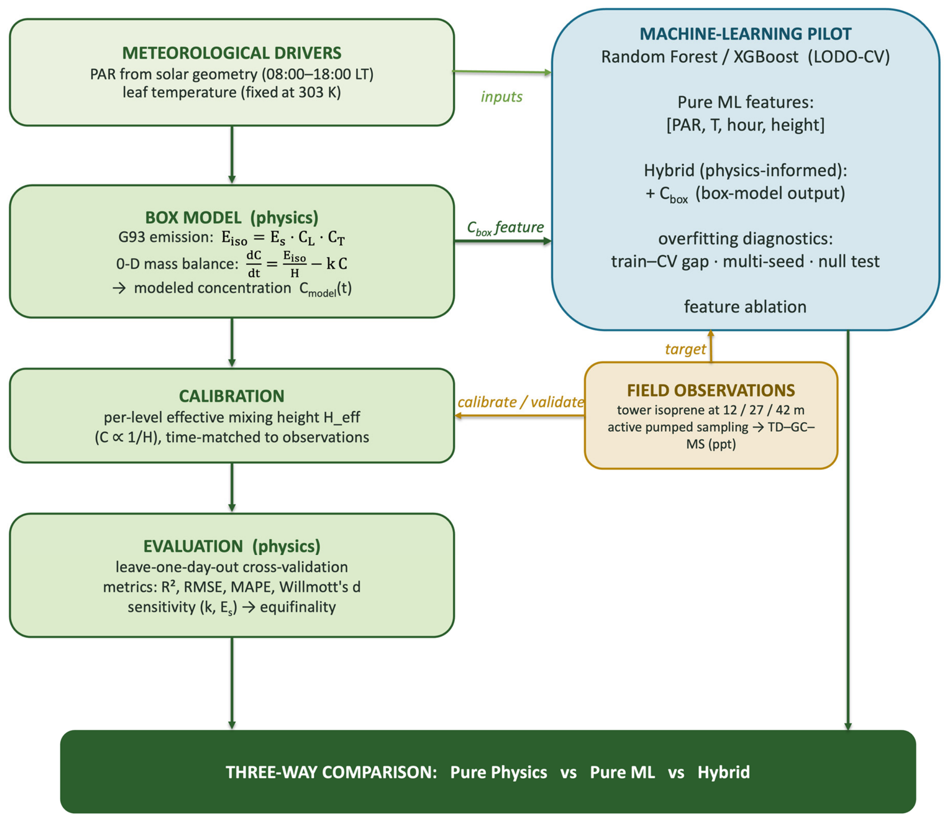
Figure 2.
Location of the study site: (a) regional setting in mainland Southeast Asia with Thailand highlighted and the study region boxed, (b) zoom of northern Thailand showing the deciduous dipterocarp forest study site at the University of Phayao (19°02′ N, 99°54′ E), (c) photograph of the 42 m micrometeorological flux tower at the Dry Dipterocarp Forest Flux Phayao (DPT) site, which carries the isoprene air-sampling ports at 12, 27, and 42 m. The red star denotes the study-site location.
2.2. Air Sampling and Chemical Analysis
Ambient air was collected on stainless-steel sorbent tubes packed with Tenax TA and Carbograph 5TD, Markes International, Llantrisant, UK adsorbents by active (pumped) collection using a portable, calibrated, mass-flow-controlled air-sampling pump (Gilian GilAir Plus STP, Sensidyne, St. Petersburg, FL, USA) that drew a fixed volume of 6 L of air per sample, adjusted to standard temperature and pressure conditions. This two-bed configuration (Tenax TA backed by Carbograph 5TD) is designed to retain very volatile compounds such as isoprene, mitigating breakthrough concerns. To capture the vertical structure of canopy isoprene, samples were taken at three fixed tower heights—12, 27, and 42 m—designated in the source dataset as below canopy, canopy, and above canopy, respectively. These ports bracket the local canopy at the tower; although the stand-average canopy height is about 16 m (Section 2.1), the port designations follow the source dataset, in which the 27 m level is taken as the canopy reference to represent the taller emergent dipterocarps at the tower. Sampling at multiple heights was adopted because the single sampling tower at the site, the variable stature of the dominant trees, the sloping terrain, and the predominantly horizontal advection of air imply that the layer of maximum isoprene mixing ratio may occur at different heights. The broader wet-season campaign deployed approximately 99 tubes across the three northerns Thailand forest types (~33 per site) [16], of which 33 were deployed at the Phayao DDF analyzed here (a corresponding dry-season campaign, January 2021, was conducted separately). Because a single pump was available, the three heights were sampled sequentially rather than synchronously: the pump was rotated among the 12, 27, and 42 m ports in consecutive ~30 min deployments (typically two to three consecutive samples at one height before moving to the next), yielding 11 tubes per height over the four days. After excluding three field blanks, 30 valid samples remained (10 per height). Field quality control was limited to these three blanks; duplicate and breakthrough samples were not collected, a limitation of this exploratory campaign noted in Section 4. The remaining tubes of the wet-season campaign belong to the other two forest types and are not analyzed here. The present study analyzes the wet-season DDF dataset; the field campaign and model configuration are summarized in Table 1.
Table 1.
Field campaign and model configuration summary.
Sorbent tubes were shipped to the Guenther laboratory (Department of Earth System Science, University of California, Irvine, CA, USA), where isoprene was quantified by thermal-desorption gas chromatography–mass spectrometry (TD–GC–MS). The sorbent tubes were thermally desorbed using a TD autosampler (ULTRA-xr, Markes International, Llantrisant, UK) into a GC (Agilent Technologies Model 7890B, Santa Clara, CA, USA) coupled to a Time of Flight Mass Spectrometer (TOF-MS, BenchTOF-Select, Markes International, Llantrisant, UK) and a Flame Ionization Detector (FID; integral to the Agilent 7890B gas chromatograph). Isoprene was identified using retention time and TOF-MS spectra and quantified using FID by comparison to an authentic isoprene standard (Apel-Riemer Environmental Inc., Miami, FL, USA, 5% accuracy). Additional details of the analytical approach are described by Nagalingam et al. 2022 [17]. Concentrations are reported as volume mixing ratios in parts per trillion (ppt).
Each sample was collected over a 30 min window (one sample of 43 min) at a nominal flow rate of 200 mL min−1, yielding a fixed volume of 6 L; the start and end times, air temperature, and sky condition were recorded for every sample. Observed level means (±standard deviation) were 2285 ± 430 ppt (12 m, below canopy), 2217 ± 554 ppt (27 m, canopy), and 1980 ± 523 ppt (42 m, above canopy); the overall mean was 2161 ± 505 ppt. The actual sampling date, time window, air temperature, and sky condition recorded for each sample were used for the time-matched model comparison.
2.3. Box-Model Formulation
The box-model simulations of isoprene emission variations were based on the G93 algorithm [5]:
where is the standard emission factor and and are dimensionless light and temperature activity factors. A generic canopy-scale standard emission factor, = 1.2 mg m−2 h−1, was adopted from the literature [7]; because the calibration constrains only the ratio /(kH) (Section 3.3), the absolute value of does not affect the model’s predictive skill. No species-specific emission-factor measurements exist for the dominant DDF taxa of northern Thailand (S. obtusa, S. siamensis, D. tuberculatus) or for the local Quercus species; enclosure studies in a Malaysian dipterocarp forest found the dipterocarps themselves to be non-emitters [18]. In the absence of local measurements, a generic canopy-scale value was adopted; the equifinality result (Section 3.3) shows that this choice does not affect predictive skill, although it precludes attribution of the emission to particular species. Leaf-level enclosure measurements of the dominant local taxa—particularly the oaks—are an important target for future work. The light activity factor was implemented as a saturating (non-rectangular-hyperbola) light response adopted from the source methodology rather than the exponential-saturation form of the original G93 algorithm.
with f = 0.385, L1 = 105.6, and L2 = 6.12, where I is PAR [18]. These coefficients follow the non-rectangular-hyperbola light-response parameterization adopted in the source methodology of the underlying dataset [15], which was fitted to reproduce the saturating PAR response of isoprene emission reported by Guenther et al. [5,19]; they are empirical constants, and their absolute values do not affect the calibrated model because any multiplicative bias is absorbed by Heff (Section 3.3). The temperature activity factor was
with = 95,000 J mol−1, = 231,000 J mol−1, T3 = 311.83 K, R = 8.314 J mol−1 K−1, and a reference and (constant) leaf temperature = = 303.15 K, giving a constant ≈ 0.93. Because leaf temperature is held constant, does not vary, so the modeled emission—and therefore the simulated concentration—is effectively driven by PAR alone; the temperature dependence of the G93 algorithm is retained for generality but remains inactive under the present forcing. Leaf temperature was fixed because continuous leaf- or air-temperature measurements coincident with the sampling were not available; the value of 303.15 K corresponds to the G93 standard temperature and lies within the narrow range of air temperatures observed during sampling (27–30 °C). Given this narrow range, the variation in that would result from using ambient temperature is small (≈10–15%), and the residual analysis (Figure S3) suggests no systematic temperature-dependent bias within the sampled conditions. Under substantially hotter or cooler conditions, however, this simplification would no longer be acceptable. Because is constant, any temperature-driven emission variability is transferred into the calibrated Heff, reinforcing its interpretation as a lumped parameter rather than a physical mixing depth.
PAR was represented by a clear-sky diurnal profile derived from solar geometry (solar declination, hour angle, and zenith angle) for the site latitude [20], restricted to the photosynthetically active window 08:00–18:00 local time. Ambient concentration was obtained from a 0-D mass balance with a first-order daytime chemical sink (reaction with OH) [21]:
where H is an effective mixing height and τ is the daytime isoprene lifetime, set to a nominal 1.5 h, consistent with a daytime OH concentration of ~1.5–2 × 10⁶ molecules cm−3 and the isoprene–OH rate constant of ≈1.0 × 10⁻¹⁰ cm3 molecule−1 s−1 [20]; reported daytime lifetimes span roughly 0.5–3 h (and longer under low-OH conditions), and this full range is explored in the sensitivity analysis (Section 2.5), which shows that cross-validated skill is optimal near the nominal value. The equation was integrated per day over the daytime window. Each day was integrated from a near-zero pre-dawn initial concentration. This choice reflects the light-dependent nature of isoprene emission—which ceases at night—combined with continued nocturnal losses (reaction with NO3 and O3, dry deposition, and boundary-layer ventilation), which are expected to deplete residual isoprene over the ~14-h nighttime gap; even for a nighttime lifetime of a few hours, less than a few percent of the evening concentration would survive until morning. The simulated evening decline likewise follows the decay of PAR-driven emission against continued chemical loss. We emphasize, however, that no nighttime observations are available to constrain these assumed features, and nocturnal chemistry is outside the scope of the present daytime model. Mass concentrations were converted to mixing ratios using the molar mass of isoprene (68.12 g mol−1); at 25 °C and 1 atm, 1 ppt ≈ 2.78 × 10⁻³ µg m−3.
2.4. Calibration and Cross-Validation
Because the box model is linear in the source term, the modeled concentration scales inversely with H (C ∝ 1/H). An effective mixing height Heff was therefore calibrated in closed form for each canopy level by minimizing the root-mean-square error against the time-matched observations. Model skill was assessed with a leave-one-day-out cross-validation (LODO-CV): in each of four folds, one day was withheld, Heff was calibrated on the remaining three days, and the held-out day was predicted. Out-of-sample predictions were pooled across folds. This design limits temporal leakage (samples from the same day never appear in both training and test sets). This is because the clear-sky forcing renders the four days nearly interchangeable; however, it primarily tests whether the model overfits the within-day accumulation signal rather than its ability to predict a genuinely novel day [22].
Performance was quantified with a comprehensive set of metrics: mean bias error (MBE), mean absolute error (MAE), root-mean-square error (RMSE) [23] with its systematic and unsystematic components, normalized mean bias and error (NMB and NME), mean absolute percentage error (MAPE), Pearson correlation (r), the Nash–Sutcliffe efficiency (NSE), reported throughout as “R2” and equal to the squared Pearson correlation only for an unbiased 1:1 fit (negative values indicate performance worse than the observed mean) [24], the Willmott index of agreement (d) [25], the ordinary-least-squares regression slope and intercept, and the two-tailed significance (p-value) of the correlation.
2.5. Structural Sensitivity Analysis
At a daytime quasi-steady state, the modeled concentration reduces to
so that C depends on the model parameters only through the ratio /(k·H). Three experiments were performed: (A) sweeping the lifetime τ (i.e., k) and recalibrating Heff at each value; (B) sweeping and recalibrating Heff; and (C) a one-at-a-time (OAT) normalized sensitivity at fixed H, perturbing Es and τ by ±20% and computing the normalized sensitivity coefficient:
2.6. Machine Learning and Hybrid Models
Two tree-based regressors were used: Random Forest (RF) [26] and Gradient-Boosted Trees (XGBoost) [27]. Each learns a nonlinear mapping from a feature vector to the isoprene concentration:
Two feature sets were compared—a pure data-driven set and a physics-informed (hybrid) set:
where is the box-model concentration computed at a fixed reference height (uncalibrated, i.e., independent of the observations), a deterministic physical feature with no data leakage. The target was the observed concentration, and all models were trained and evaluated under the identical LODO-CV protocol and compared with the box-model baseline.
Given the small sample (n = 30, four days), overfitting was controlled through several measures, all fixed a priori (not tuned on the test folds): (i) shallow, capacity-limited trees (RF: max_depth = 3, min_samples_leaf = 3, max_leaf_nodes = 8, max_features = 0.6; XGBoost: max_depth = 2, learning_rate = 0.05, min_child_weight = 3, and gamma = 0.5); (ii) explicit regularization (XGBoost L2 reg_lambda = 2.0 and L1 reg_alpha = 0.5; RF bootstrap and feature subsampling); (iii) multi-seed averaging of predictions across random states to reduce variance; (iv) reporting of the train-versus-CV R2 gap as a direct overfitting diagnostic; (v) out-of-bag (OOB) scoring for RF; and (vi) a permutation null test in which the target was shuffled and the full LODO-CV repeated [28]. Feature standardization was not applied because tree ensembles are invariant to monotonic feature scaling. An ablation experiment compared four feature sets, base [PAR, T, height], base + hour, base + , and base + hour + , to isolate the value of the physical feature; its added value was quantified as the change in cross-validated skill:
All analyses were implemented in Python 3.11.13 using NumPy 2.0.1, pandas 2.2.2, scikit-learn 1.5.1 [29], XGBoost 2.1.0 [27], and Matplotlib 3.9.1 [30].
3. Results
We first evaluate the calibrated box model against the time-matched tower observations, its vertical structure, in-sample fit, and cross-validated skill, then examine parameter identifiability through a structural sensitivity analysis, and finally benchmark the physical model against tree-based machine learning. In brief, the box model reproduces the mean daytime level and diurnal accumulation shape with cross-validated R2 = 0.64–0.68 and MAPE ≈ 11%; the near-identical per-level effective mixing heights indicate a well-mixed canopy layer with only a weak vertical gradient. The sensitivity analysis indicates that the emission factor, loss rate, and mixing height are identifiable only through the ratio Es/(kH), so predictive skill is insensitive to the adopted literature values. The machine-learning benchmark recovers the skill lost without temporal information when the box-model output is supplied as a feature, but this feature proves equivalent to a simple time-of-day predictor, indicating that the box model performs on par with a diurnal-climatology baseline while retaining mechanistic interpretability.
3.1. Box-Model Performance and Vertical Structure
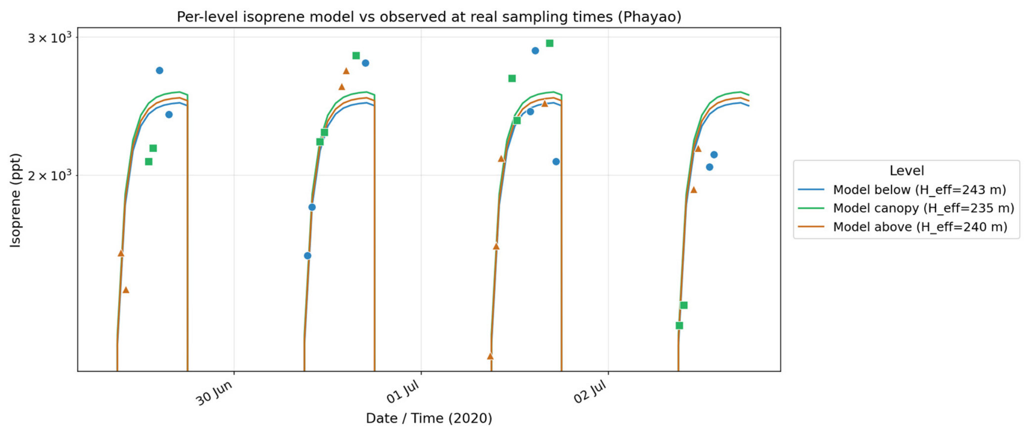
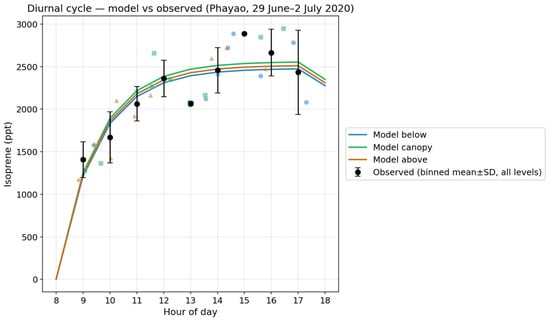
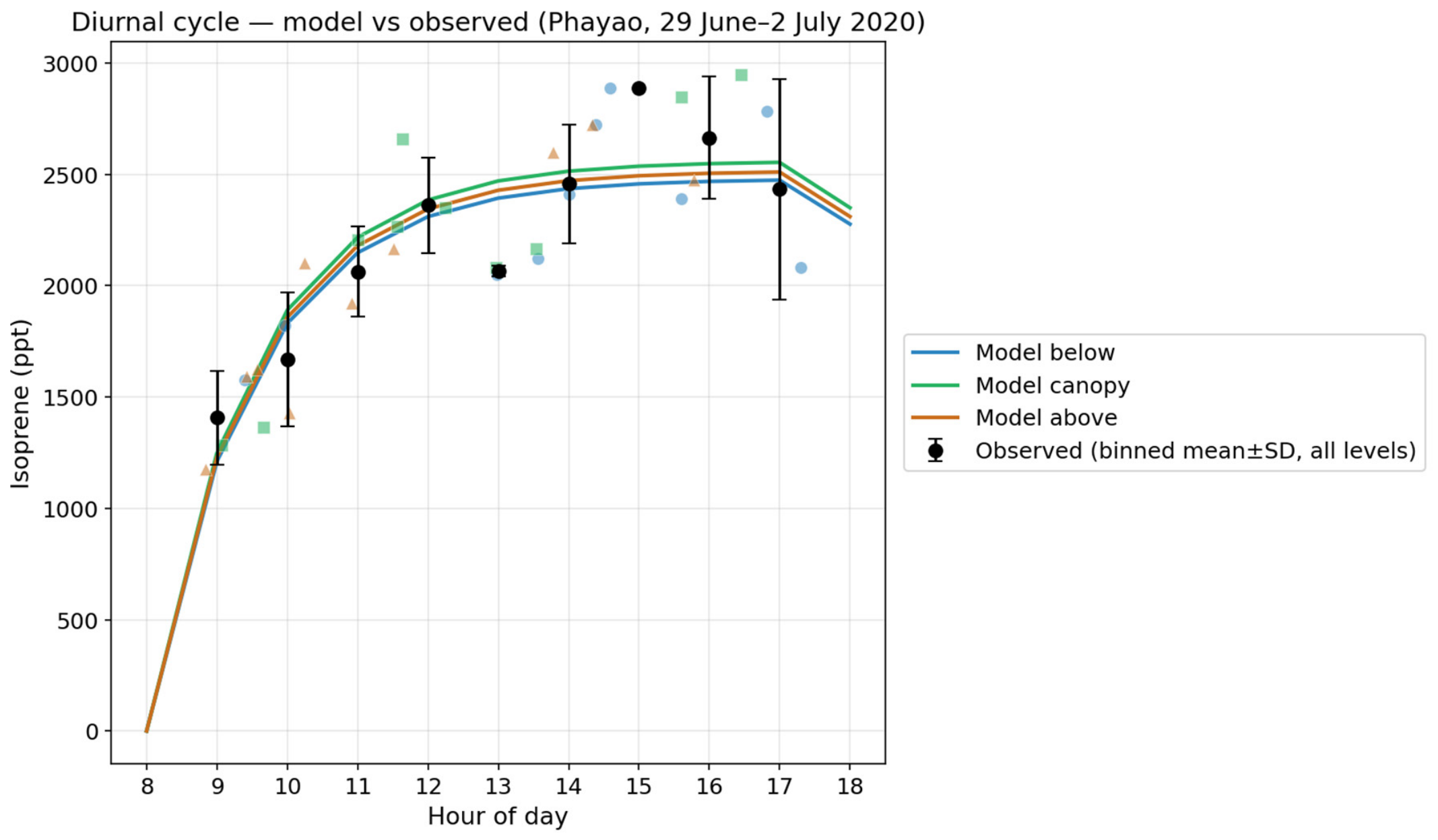
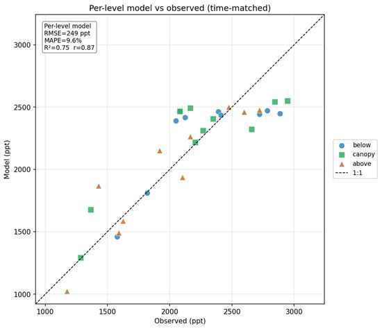
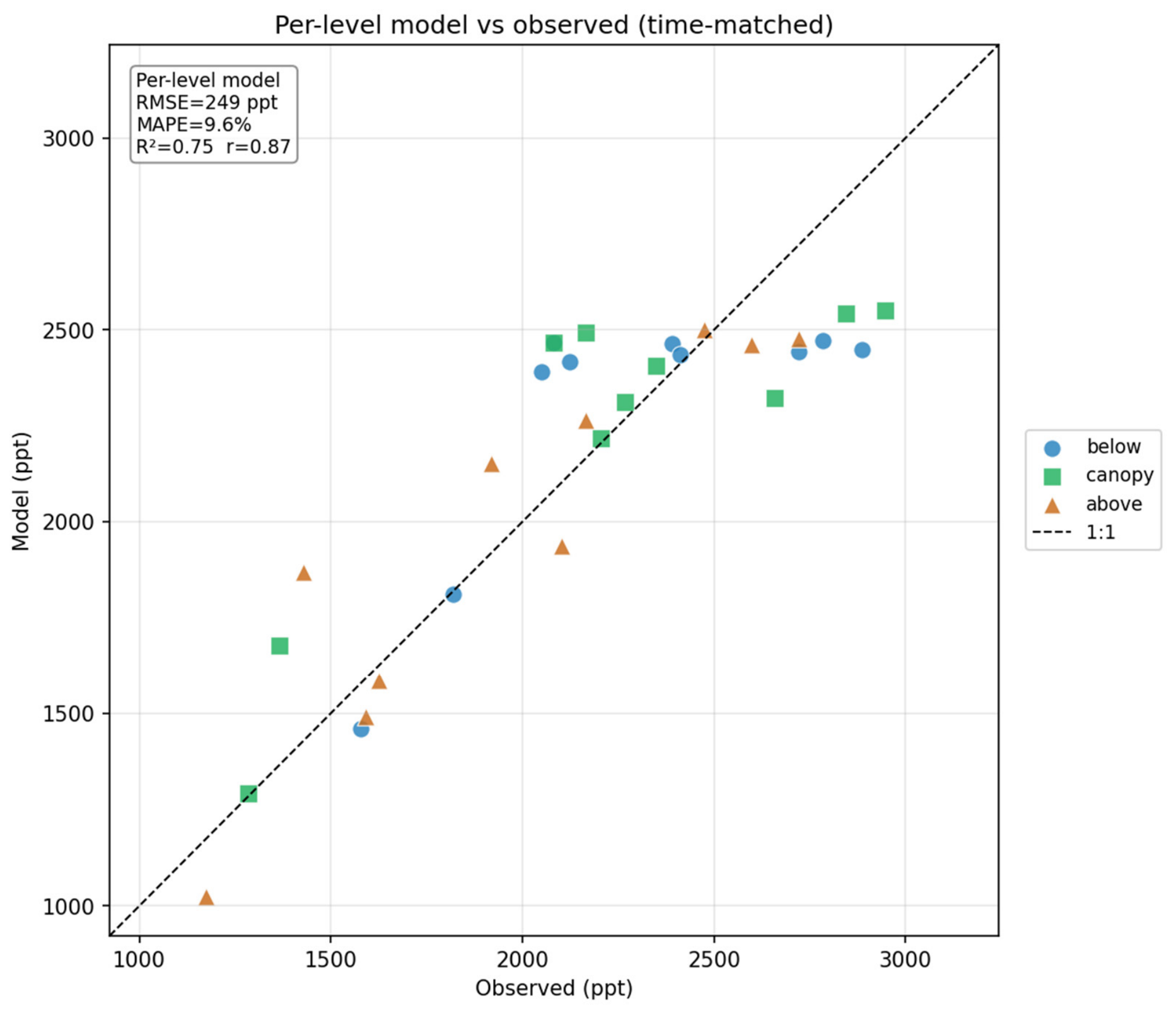
When matched to observations at their actual sampling times, the calibrated box model reproduced the observed diurnal accumulation: low concentrations in the morning rising to an afternoon plateau (Figure 3 and Figure 4). Because the clear-sky PAR forcing varies little between days, this time-matched agreement primarily reflects the within-day (morning-to-afternoon) accumulation signal rather than day-to-day variability. In-sample agreement was strong (R2 = 0.75; r = 0.87; RMSE = 251 ppt; MAPE = 9.6%; MBE ≈ +1 ppt; Willmott’s d = 0.92; p < 0.001). Calibrating an effective mixing height separately for each level produced nearly identical values (Heff = 235–243 m), and per-level skill increased with height: R2 = 0.56 (12 m), 0.75 (27 m), and 0.84 (42 m). The near-constancy of Heff across levels indicates that the vertical concentration gradient (below > canopy > above, differing by only ~15%) is small relative to diurnal variability, supporting the well-mixed 0-D assumption (Table 2 and Table 3; Figure 5).
Figure 3.
Time series of modeled (lines) and observed (markers) isoprene at three tower heights, matched to actual sampling times over the four-day campaign (29 June–2 July 2020). Colors denote the three levels—blue, below canopy (12 m); green, canopy (27 m); and orange, above canopy (42 m)—with observations shown as circles, squares, and triangles, respectively, and the corresponding calibrated effective mixing heights (Heff) given in the legend. The vertical (isoprene) axis is on a logarithmic scale.
Figure 4.
Mean diurnal cycle: modeled hourly profiles (lines) versus hour-binned observations (mean ± SD, black markers) over the four-day campaign (29 June–2 July 2020). Colors denote the three levels (blue, below canopy; green, canopy; orange, above canopy); the black markers show the hourly binned mean ± standard deviation across all levels, and the faint colored markers show the individual observations.
Table 2.
Observed isoprene concentration by tower height (ppt).
Table 3.
Per-level calibration of the effective mixing height (Heff) and time-matched statistical evaluation of the box model (in-sample). Units: ppt unless stated. Note: For out-of-sample skill see Section 3.2: leave-one-day-out R2 = 0.64–0.68, RMSE ≈ 282–297 ppt, MAPE ≈ 11%.
Figure 5.
Modeled versus observed isoprene (1:1 scatter), colored by tower height (time-matched).
3.2. Cross-Validated Skill
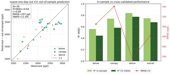
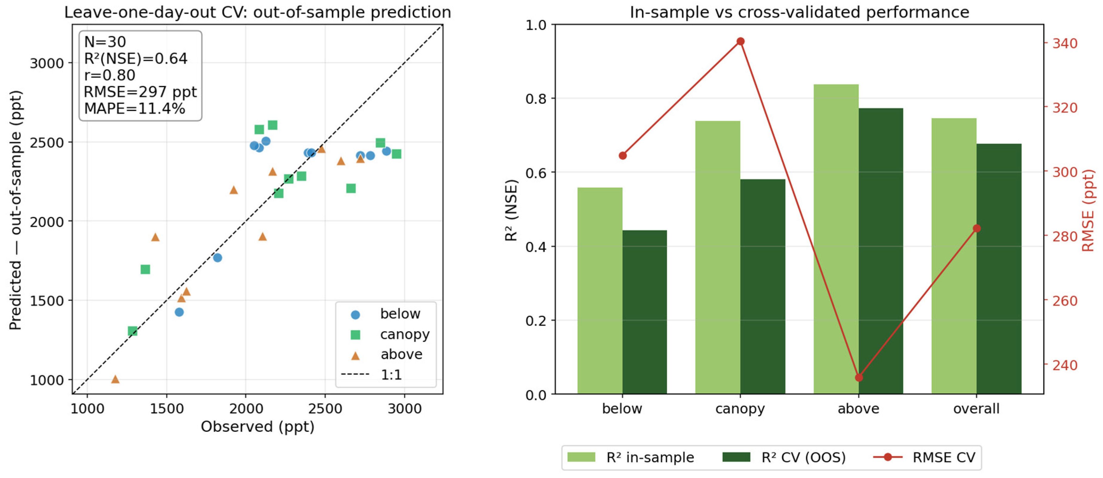
Under LODO-CV, Heff remained stable across folds (234–249 m), and the optimism gap between in-sample and out-of-sample skill was modest. The pooled out-of-sample performance was R2 (NSE) = 0.64, r = 0.80, RMSE = 297 ppt, MAPE = 11.4%, and MBE = −11 ppt for the per-level model; a single-box variant gave R2 = 0.68 (RMSE = 282 ppt). The small in-sample-to-CV decrease (0.75 to 0.64, and to 0.68 for the single-box variant) indicates that the model does not overfit the within-day accumulation signal; because the clear-sky forcing makes the four days nearly interchangeable, this should not be read as demonstrated skill in predicting a genuinely novel day (Figure 6). Additional error diagnostics, a residual analysis, a Taylor diagram, and a Bland–Altman comparison are provided as Supplementary Material (Figures S1–S3) and indicate near-normal, largely unbiased residuals with all paired model–observation differences falling within the limits of agreement.
Figure 6.
Leave-one-day-out cross-validation: (left) out-of-sample predicted versus observed; (right) in-sample versus cross-validated R2 and RMSE.
3.3. Sensitivity and Parameter Identifiability
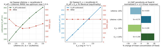
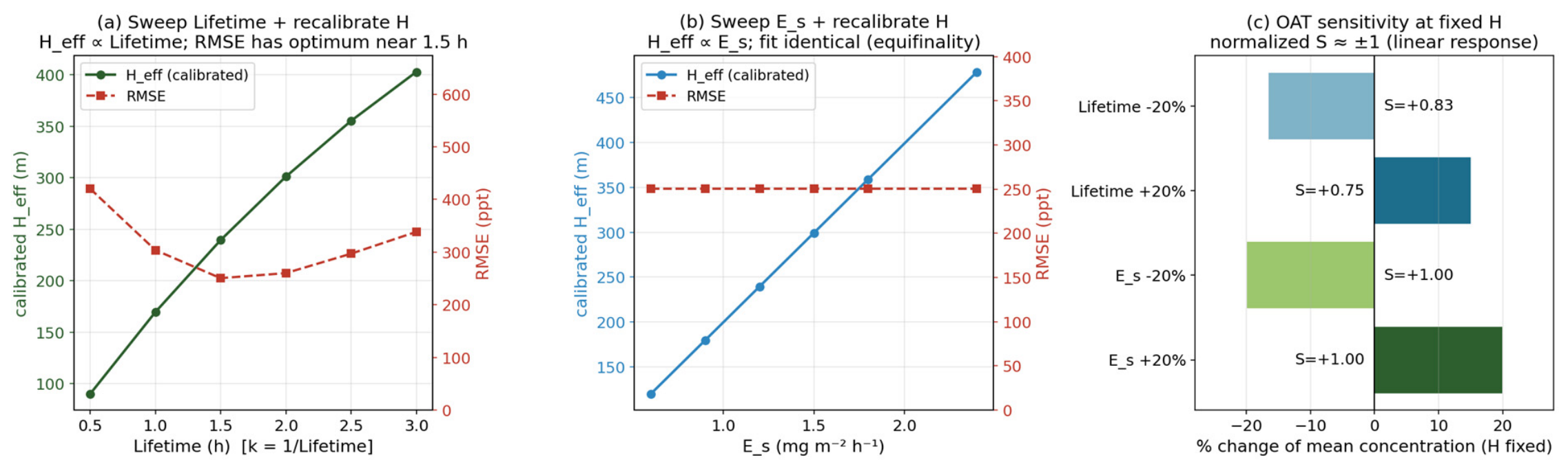
The lifetime sweeps with recalibration (Figure 7a) showed that Heff scales approximately linearly with τ, while cross-validated skill exhibited a clear optimum near τ = 1.5 h (R2 declining to 0.28 at τ = 0.5 h and 0.54 at τ = 3.0 h), consistent with the literature on daytime lifetime. The Es sweep (Figure 7b) left all fit statistics unchanged while Heff scaled exactly in proportion to Es, demonstrating complete equifinality between Es and H. The OAT analysis at a fixed H (Figure 7c) gave a normalized sensitivity of S = +1.00 for Es and S ≈ +0.75 to +0.83 for τ, i.e., an approximately linear response. Together these results show that the parameters Es, k, and H are identifiable only through the ratio Es/(kH); consequently, predictive skill is insensitive to the specific literature values adopted for Es and τ, which can be fixed safely, with Heff absorbing the combined uncertainty.
Figure 7.
Structural sensitivity analysis: (a) lifetime sweep with H recalibration; (b) Es sweep with H recalibration (equifinality); (c) one-at-a-time normalized sensitivity at fixed H. The bar colors merely distinguish the four perturbations (Lifetime and Es, each ±20%), which are labeled directly together with their normalized sensitivity coefficients (S); the colors carry no additional meaning.
3.4. Machine-Learning Benchmark and the Value of Physics
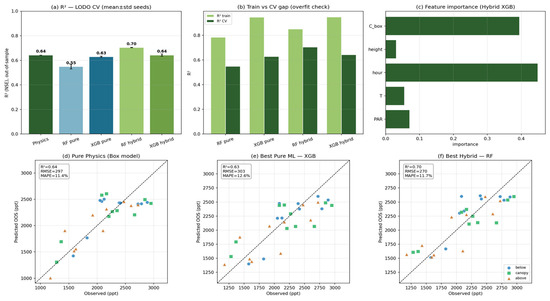
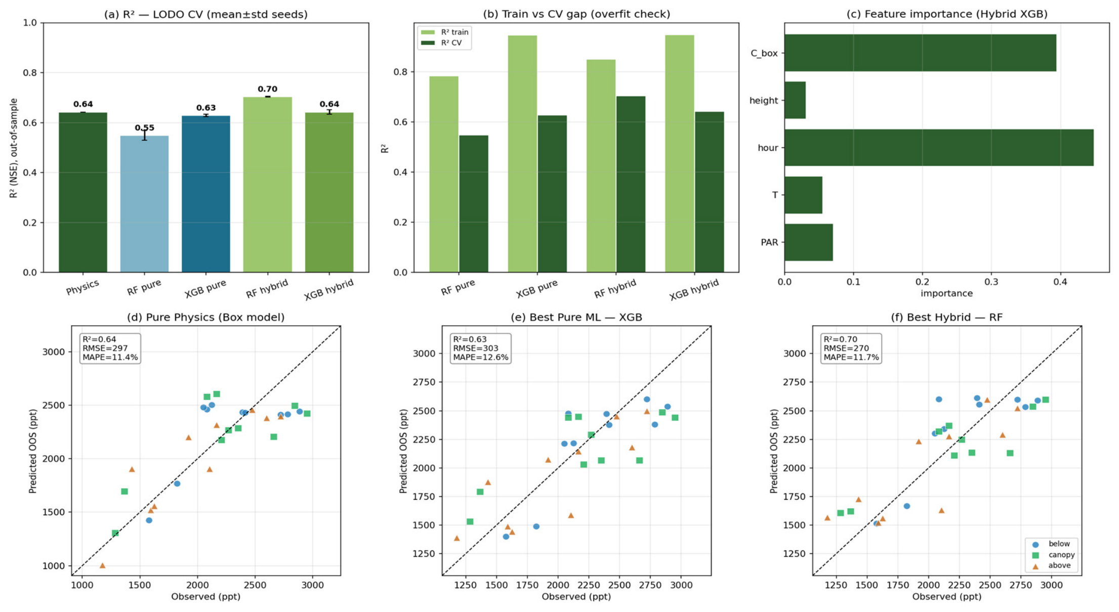
Under the identical LODO-CV protocol and conservative regularization, the five approaches gave comparable out-of-sample skill (Table 4; Figure 8). The hybrid Random Forest performed best (R2 = 0.70, RMSE = 270 ppt), followed by the box model, hybrid XGBoost, and Pure XGBoost (R2 = 0.63–0.64); Pure Random Forest was the lowest (R2 = 0.55). The XGBoost variants showed a systematic low bias (−62 to −64 ppt; Table 4), a tendency of boosted trees to under-predict with so few training samples, whereas the Random Forests were essentially unbiased. Overfitting diagnostics were favorable: the seed-to-seed standard deviation of R2 was ≈0.01 (stable results), train-to-CV gaps were 0.15–0.32 (limited overfitting), and the permutation null test produced strongly negative R2 (≈−0.4), suggesting that the models did not fit noise. In the hybrid models, the two most important features were the hour of day and Cbox (importance ≈ 0.39–0.45 each), indicating that the box-model output carries a predictive signal; because Cbox is generated from a deterministic clear-sky PAR curve, however, this signal is largely time-of-day information, as the ablation suggests (Table 5).
Table 4.
Cross-validated (leave-one-day-out) comparison of Pure Physics, Pure ML, and hybrid (physics-informed) models, with overfitting diagnostics. R2 is the Nash–Sutcliffe efficiency on pooled out-of-sample predictions.
Figure 8.
Machine-learning comparison: out-of-sample R2, train-vs-CV overfitting check, feature importance, and prediction scatter for Pure Physics, Pure ML, and hybrid models.
Table 5.
Feature ablation: out-of-sample (LODO-CV) R2 for four feature sets and two ML models (base = [PAR, T, height]). Adding the physical feature recovers skill lost when the explicit time feature is withheld. A check mark (✓) indicates that the feature (Hour or ) is included in the feature set, and an em dash (—) indicates that it is not; in the “Random Forest” and “XGBoost” columns, “—” denotes not applicable (the box model is a single physics-based estimate and is not run with either machine-learning algorithm). Negative R2 values indicate performance worse than predicting the observed mean.
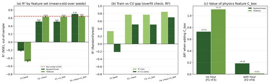
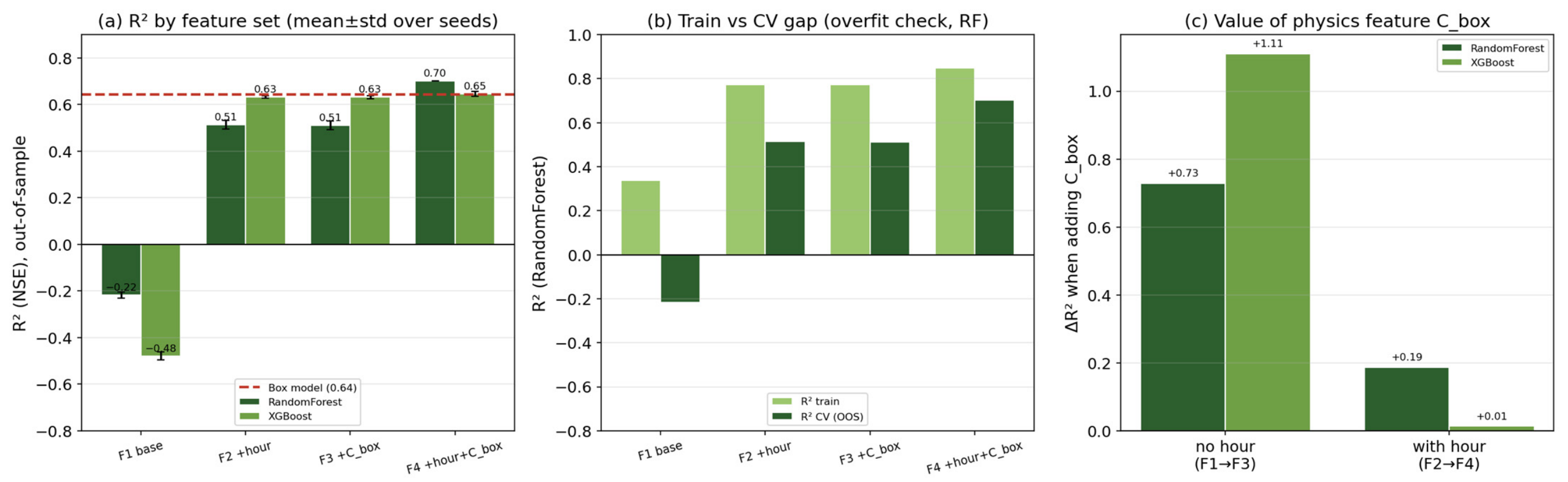
The ablation experiment (Table 5; Figure 9) made the role of physics explicit. With only instantaneous drivers [PAR, T, height] and no temporal information, both ML models failed (R2 = −0.22 for RF and −0.52 for XGBoost), worse than predicting the mean, because the symmetric PAR profile cannot distinguish morning from afternoon at equal radiation. Adding the single physical feature raised R2 by +0.73 (RF) and +1.16 (XGBoost), recovering performance comparable to, or better than, the box model itself. Adding the explicit hour feature had a similar effect, and combining both was largely redundant, because hour and encode the same diurnal accumulation information. In other words, because derives from a deterministic clear-sky PAR curve, it functions here mainly as an encoding of time of day rather than as independent physical information. Because the hour-only model is equivalent to a diurnal climatology, the box model does not outperform this simple temporal baseline in predictive skill; its value lies instead in interpretability and mechanistic transparency.
Figure 9.
Feature ablation: (a) R2 by feature set with box-model reference; (b) train vs. CV gap; (c) the value of the physical feature (ΔR2 with and without the explicit hour feature).
4. Discussion
This pilot study suggests that a deliberately simple, interpretable box model can reproduce the mean level and diurnal accumulation shape of daytime canopy isoprene at a tropical DDF tower with cross-validated R2 ≈ 0.64–0.68 and MAPE ≈ 11% using only PAR, temperature, and a calibrated effective mixing height. The strict leave-one-day-out design and the small optimism gap indicate that the model does not overfit the within-day accumulation signal. This is because the near-invariant clear-sky forcing makes the four sampling days nearly interchangeable; however, this is not evidence of skill in predicting a genuinely novel day, and day-to-day predictive skill remains untested with the present forcing. Diagnostic checks nonetheless revealed a mild tendency to underestimate the highest concentrations (regression slope ≈ 0.74), consistent with partial regression-to-the-mean and with the idealized clear-sky PAR profile that smooths genuine midday peaks; the model is therefore most reliable for typical daytime levels and slightly conservative at the upper extreme. Moreover, because the near-invariant forcing produces almost no modeled day-to-day variability, the genuine day-to-day and sampling variance in the observations is structurally uncapturable, which sets an upper bound on the achievable R2.
The analysis shows that Es, k, and H are identifiable only through the ratio Es/(kH) (structural non-identifiability or equifinality [31]). Because the steady-state concentration depends only on Es/(kH), the absolute values of the emission factor and chemical lifetime cannot be inferred from concentration data when H is free; conversely, the model’s predictive skill is robust to the literature values chosen for these parameters. The effective mixing height should therefore be interpreted as a lumped calibration parameter (numerically Eiso/(k·Cobs)) that absorbs uncertainty in emission strength, chemistry, and dilution, and should not be read as a physical mixed-layer depth but rather as as a directly measurable physical depth. The emergence of a cross-validation optimum near τ = 1.5 h is nonetheless reassuring, as it coincides with the independently established daytime isoprene lifetime and is governed by the shape of the diurnal accumulation curve rather than its magnitude.
The ML pilot clarifies the relationship between physics and data-driven modeling. Pure ML with only instantaneous inputs fails because it lacks the temporal information that governs isoprene accumulation, whereas supplying either the box-model output () or an explicit hour-of-day feature restores essentially all skill. As the ablation shows (Table 5), and hour-of-day carry equivalent information here— is effectively a physically shaped re-encoding of time of day—so the result suggests the value of a temporal or accumulation feature rather than any superiority of physics over data, consistent with the broader interest in hybrid, physics-guided modeling [10,11,32]. Where explicit time stamps are available, a simple time feature can substitute for the physical feature; the box model nonetheless offers advantages in interpretability and in encoding the accumulation process from first principles. Between the two learners, Random Forest slightly outperformed XGBoost in the full hybrid configuration (R2 = 0.70 vs 0.65), as expected for a very small dataset in which bagging is typically more robust to overfitting than boosting.
The systematic increase in model skill with height (R2 = 0.56, 0.75, and 0.84 at 12, 27, and 42 m) is physically reasonable. Above the canopy, the air is more efficiently mixed, and the concentration reflects an integrated, ecosystem-scale signal that matches the well-mixed box assumption [33]. Below the canopy, concentrations are shaped by local, poorly mixed processes that a 0-D model cannot represent—heterogeneous nearby sources, weak and intermittent within-canopy turbulence [34], and possible deposition or chemical losses on foliage [6,20]—so the below-canopy time series carries larger stochastic variability relative to its diurnal signal. The greater scatter (not bias) of the below-canopy residuals supports this interpretation.
Several limitations temper these conclusions and motivate the pilot framing. First, the validation rests on 30 discrete adsorbent-tube samples from four consecutive days in a single (wet) season, collected without duplicate or breakthrough checks, so seasonal generalization is untested—although a paired dry-season campaign exists and is a natural next step; the negative-to-modest spread of per-level skill (especially the lower R2 below canopy) likely reflects sub-canopy heterogeneity and sampling noise. We also note that the below-/at-/above-canopy designations and their tower heights (12/27/42 m) follow the original dataset and that the canopy height adopted here (~16 m [12]) is taken from the site literature rather than re-surveyed in this study. Second, PAR was represented by an idealized clear-sky profile rather than measured radiation. This is the most consequential simplification of the study: it suppresses genuine day-to-day variability, renders the four sampling days nearly interchangeable in the model, weakens the meaning of the cross-validation, and may flatter the diurnal fit, since days with substantial cloud cover would depart from the assumed profile. Observed sky conditions during sampling ranged from partly cloudy to cloudy, so actual PAR was certainly below the clear-sky ideal for part of the campaign; the calibrated Heff implicitly absorbs the resulting mean bias, but the day-specific errors cannot be corrected. Incorporating measured or reanalysis radiation (e.g., ERA5/MERRA-2) is therefore the single highest-priority improvement for future work. Third, the standard emission factor was taken from the literature rather than measured locally, and leaf temperature was held constant, which neglects the known sensitivity of emission capacity to leaf temperature and heat stress [18]; reassuringly, residuals showed no systematic dependence on air temperature over the observed 27–30 °C range or on sky condition (Figures S1–S3), indicating that this simplification introduced no detectable bias within the sampled conditions, though it may become important over a wider temperature range. Fourth, the 0-D framework cannot resolve the (weak) vertical gradient; a physically resolved profile would require micrometeorological inputs (e.g., friction velocity, eddy diffusivity) [33] that were unavailable. Moreover, the chemical sink is represented as a single first-order daytime loss to OH, and the model is confined to the 08:00–18:00 window: nighttime chemistry—notably oxidation by NO3, together with deposition and boundary-layer dynamics—is not represented, and the nocturnal evolution of isoprene between 18:00 and 08:00 is unconstrained by observations. Extending the framework to the full diel cycle, with nighttime measurements and an explicit NO3/O3 sink, is an important direction for future work [20]. Finally, the ML results are exploratory: although diagnostics indicate limited overfitting and stable, signal-driven predictions, four folds provide a high-variance estimate, and larger campaigns are needed before drawing firm comparative conclusions.
Beyond the methodology, the results carry implications for the DDF context of northern Thailand. The estimated canopy mixing ratios (of the order of 2000 ppt, i.e., ~2 ppb, during the daytime maximum) suggest that this ecosystem is an active isoprene source when foliage is photosynthetically active. Notably, the dominant dipterocarps are generally not significant isoprene emitters; leaf-level enclosure measurements in a dipterocarp forest detected isoprene emission only from a non-dipterocarp component [18], implying that the co-occurring oaks (Quercus spp.)—characteristically strong isoprene emitters—are the more likely source at this site, a clear example of a minor floristic component dominating a forest’s isoprene emission [35]. Ecologically, the observed canopy mixing ratios (~2000 ppt) during the early wet season are consistent with the phenology of this ecosystem: sampling coincided with fully expanded, photosynthetically active foliage following leaf flush [13], when both light-dependent isoprene synthesis [2] and leaf area are near their seasonal maximum. The weak vertical gradient (below > canopy > above, ~15%) suggests an elevated source region within the upper canopy combined with efficient daytime vertical mixing, consistent with within- and above-canopy gradients reported for a Bornean rainforest [35]. Pronounced seasonality is expected—near-zero emission in the leafless late dry season, rising rapidly through leaf flush—as documented for other tropical forests [36], and the dry-season companion dataset [16] offers a direct test of this expectation. The estimated mixing ratios are comparable to canopy-level values reported for other tropical forests, for example, ~1000–3000 ppt above a Southeast Asian rainforest during OP3 in Borneo [35] and ~1–5 ppb over the Amazon [36], indicating that the calibrated estimates are physically plausible despite the reduced-complexity framework. The strongly seasonal, deciduous nature of DDFs nonetheless distinguishes it from these evergreen systems, underscoring the need for phenology-resolved comparisons. Because isoprene reacts rapidly with OH to form ozone and secondary organic aerosol [2,3,20], even a first-order quantification is relevant to the region’s well-documented dry-season air-quality burden [8], where biogenic emissions act on top of biomass burning and anthropogenic precursors. We note that the site lies on a university campus near the town of Phayao, with agricultural land and seasonal biomass burning in the wider area [8]; associated NOx emissions can modulate isoprene chemistry directly and through ozone formation [9,21]. Such influences were likely modest during the wet-season campaign but should be quantified—ideally with co-located NOx and O3 measurements—when the framework is extended toward regional application. Resolving the seasonal phenology of DDF isoprene—particularly the contrast between the leafless dry season and the photosynthetically active wet season—is therefore a priority for regional photochemical assessment, and the present calibrated model provides a tractable starting point for incorporating biogenic isoprene into northern Thailand emission inventories. In particular, because the calibration constrains only the lumped ratio Es/(kH) and not the emission factor itself, it cannot be used to refine a MEGAN emission factor without an independent estimate of the effective mixing height and lifetime; it is better regarded as an observational constraint on the lumped ratio [1].
Despite these caveats, the workflow is simple and undemanding of data, requiring only routine meteorological drivers and a modest number of validation samples. It offers a coherent template—calibration, strict cross-validation, sensitivity and identifiability analysis, and a physics-informed ML benchmark—whose transferability to other DDFs and under-instrumented tropical forests is a prospect to be tested rather than a demonstrated property.
5. Conclusions
This pilot study provides an observation-constrained box-model estimate of canopy isoprene over a deciduous dipterocarp forest in northern Thailand. A simplified G93-based 0-D box model reproduced the observed mean level and diurnal accumulation shape with cross-validated R2 ≈ 0.64–0.68 and MAPE ≈ 11% under a strict leave-one-day-out protocol, with an effective mixing height that was stable across folds; because the clear-sky forcing makes the sampling days nearly interchangeable, this reflects a within-day accumulation signal with limited overfitting rather than demonstrated skill on genuinely novel days. A structural sensitivity analysis showed that the emission factor, chemical loss rate, and mixing height are confounded through the ratio Es/(kH), so that predictive skill is insensitive to the literature parameter values adopted. A physics-informed machine-learning pilot showed that tree-based models are competitive with the box model and that the box-model output is a high-value feature: when temporal information was withheld, this single physical feature recovered essentially all predictive skill (ΔR2 up to +1.16), an effect equivalent to that of an explicit hour-of-day feature, indicating that the two carry the same information. The results indicate that the DDF is an active daytime isoprene source whose photochemical role in northern Thailand’s seasonal air quality warrants further study. Although constrained to a four-day campaign and therefore exploratory, the work provides a low-data workflow—coupling interpretable physics with data-driven benchmarking—that could be applied to DDFs and other under-instrumented tropical forests. Future work should extend the observational base across the dry and wet seasons, incorporate measured PAR, and test the hybrid approach on larger datasets to support regional BVOC inventories. Given the four-day, single-season scope, all comparative findings should be regarded as hypothesis-generating rather than confirmatory.
Supplementary Materials
The following supporting information can be downloaded at: https://www.mdpi.com/article/10.3390/atmos17090809/s1, Figure S1: Residual diagnostics (residuals versus fitted values and hour, residual distribution, and normal Q–Q plot); Figure S2: Taylor diagram summarizing correlation, normalized standard deviation, and RMSD by tower level; Figure S3: Bland–Altman agreement analysis, and residuals versus air temperature and sky condition.
Author Contributions
Conceptualization, A.P. and T.A.; methodology, A.P., T.A., R.J., P.K. and A.G.; software, A.P. and T.A.; formal analysis, A.P., T.A. and P.K.; investigation, A.P., P.K., R.J., V.S. and R.M.; data curation, A.P., P.K. and R.J.; writing—original draft preparation, A.P. and T.A.; writing—review and editing, A.P., T.A., P.K., R.J., R.M. and A.G.; visualization, A.P. and T.A.; supervision, T.A. All authors have read and agreed to the published version of the manuscript.
Funding
This research was partially supported by the University of Phayao and the National Astronomical Research Institute of Thailand (NARIT).
Institutional Review Board Statement
Not applicable.
Informed Consent Statement
Not applicable.
Data Availability Statement
The isoprene sampling dataset analyzed in this study is available from the corresponding author upon reasonable request; the analysis code is likewise available on request.
Acknowledgments
The authors thank the ThaiFlux/AsiaFlux Dry Dipterocarp Forest Flux Phayao (DPT) site, established under the JST–JICA IMPAC-T project, and its research team for the site infrastructure and micrometeorological data. We also thank the University of Phayao and the National Astronomical Research Institute of Thailand (NARIT) for their support.
Conflicts of Interest
The authors declare no conflicts of interest.
References
- Guenther, A.B.; Jiang, X.; Heald, C.L.; Sakulyanontvittaya, T.; Duhl, T.; Emmons, L.K.; Wang, X. The Model of Emissions of Gases and Aerosols from Nature version 2.1 (MEGAN2.1): An extended and updated framework for modeling biogenic emissions. Geosci. Model Dev. 2012, 5, 1471–1492. [Google Scholar] [CrossRef] [Scilit]
- Sharkey, T.D.; Wiberley, A.E.; Donohue, A.R. Isoprene emission from plants: Why and how. Ann. Bot. 2008, 101, 5–18. [Google Scholar] [CrossRef] [Scilit] [PubMed]
- Claeys, M.; Graham, B.; Vas, G.; Wang, W.; Vermeylen, R.; Pashynska, V.; Cafmeyer, J.; Guyon, P.; Andreae, M.O.; Artaxo, P.; et al. Formation of secondary organic aerosols through photooxidation of isoprene. Science 2004, 303, 1173–1176. [Google Scholar] [CrossRef] [Scilit] [PubMed]
- Loreto, F.; Fineschi, S. Reconciling functions and evolution of isoprene emission in higher plants. New Phytol. 2015, 206, 578–582. [Google Scholar] [CrossRef] [Scilit] [PubMed]
- Guenther, A.; Zimmerman, P.R.; Harley, P.C.; Monson, R.K.; Fall, R. Isoprene and monoterpene emission rate variability: Model evaluations and sensitivity analyses. J. Geophys. Res. Atmos. 1993, 98, 12609–12617. [Google Scholar] [CrossRef] [Scilit]
- Kesselmeier, J.; Staudt, M. Biogenic volatile organic compounds (VOC): An overview on emission, physiology and ecology. J. Atmos. Chem. 1999, 33, 23–88. [Google Scholar] [CrossRef] [Scilit]
- Saito, T.; Yokouchi, Y.; Kosugi, Y.; Tani, M.; Philip, E.; Okuda, T. Methyl chloride and isoprene emissions from tropical rain forest in Southeast Asia. Geophys. Res. Lett. 2008, 35, L19812. [Google Scholar] [CrossRef] [Scilit]
- Uttamang, P.; Janta, R.; Bran, S.H.; Macatangay, R.; Surapipith, V.; Tala, W.; Chantara, S. Effects of biogenic volatile organic compounds and anthropogenic NOx emissions on O3 and PM2.5 formation over the northern region of Thailand. Front. Environ. Sci. 2023, 11, 1146437. [Google Scholar] [CrossRef] [Scilit]
- Jacob, D.J. Introduction to Atmospheric Chemistry; Princeton University Press: Princeton, NJ, USA, 1999. [Google Scholar]
- Reichstein, M.; Camps-Valls, G.; Stevens, B.; Jung, M.; Denzler, J.; Carvalhais, N.; Prabhat. Deep learning and process understanding for data-driven Earth system science. Nature 2019, 566, 195–204. [Google Scholar] [CrossRef] [Scilit] [PubMed]
- Karpatne, A.; Atluri, G.; Faghmous, J.H.; Steinbach, M.; Banerjee, A.; Ganguly, A.; Shekhar, S.; Samatova, N.; Kumar, V. Theory-guided data science: A new paradigm for scientific discovery from data. IEEE Trans. Knowl. Data Eng. 2017, 29, 2318–2331. [Google Scholar] [CrossRef] [Scilit]
- Suwannapat, P.; Sanwangsri, M.; Komori, D.; Kim, W.; Chidthaisong, A.; Cha-un, N.; Nusit, K.; Sonklin, W.; Vongruang, P.; Panya, M.; et al. Introduction to a New ThaiFlux Site: Dry Dipterocarp Forest Flux Phayao Site (DPT). In Proceedings of the AsiaFlux Workshop, Los Baños, Philippines, 18–23 August 2014. [Google Scholar]
- Bunyavejchewin, S.; Baker, P.J.; Davies, S.J. Seasonally Dry Tropical Forests in Continental Southeast Asia: Structure, Composition, and Dynamics. In The Ecology and Conservation of Seasonally Dry Forests in Asia; McShea, W.J., Davies, S.J., Bhumpakphan, N., Eds.; Smithsonian Institution Scholarly Press: Washington, DC, USA, 2011; pp. 9–35. [Google Scholar]
- Geron, C.; Owen, S.; Guenther, A.; Greenberg, J.; Rasmussen, R.; Bai, J.H.; Li, Q.-J.; Baker, B. Volatile Organic Compounds from Vegetation in Southern Yunnan, China: Emission Rates and Some Potential Regional Implications. Atmos. Environ. 2006, 40, 1759–1773. [Google Scholar] [CrossRef] [Scilit]
- Intanil, P.; Sanwangsri, M.; Boonpoke, A.; Hanpattanakit, P. Contribution of Root Respiration to Soil Respiration during Rainy Season in Dry Dipterocarp Forest, Northern Thailand. Appl. Environ. Res. 2018, 40, 19–27. [Google Scholar] [CrossRef] [Scilit]
- Kayong, P. Study of Isoprene Emission from Forests in the Upper Northern Region of Thailand. Master’s Thesis, University of Phayao, Phayao, Thailand, 2023. Available online: https://updc.up.ac.th/handle/123456789/1363 (accessed on 15 August 2026).
- Nagalingam, S.; Seco, R.; Musaev, K.; Basu, C.; Kim, S.; Guenther, A. Impact of Heat Stress on Foliar Biogenic Volatile Organic Compound Emission and Gene Expression in Tomato (Solanum lycopersicum) Seedlings. Elem. Sci. Anth. 2022, 10, 00096. [Google Scholar] [CrossRef] [Scilit]
- Saito, T.; Tomimatsu, H.; Ma, Y.; Kang, H.; Tang, Y.; Andrews, S.J.; Mohti, A. Inter-specific variation of isoprene emissions in a Southeast Asian tropical rainforest: Links to light environments and atmospheric implications. Elem. Sci. Anth 2025, 13, 000041. [Google Scholar] [CrossRef] [Scilit]
- Guenther, A.B.; Monson, R.K.; Fall, R. Isoprene and monoterpene emission rate variability: Observations with Eucalyptus and emission rate algorithm development. J. Geophys. Res. Atmos. 1991, 96, 10799–10808. [Google Scholar] [CrossRef] [Scilit]
- Iqbal, M. An Introduction to Solar Radiation; Academic Press: Toronto, ON, Canada, 1983. [Google Scholar]
- Atkinson, R.; Arey, J. Atmospheric degradation of volatile organic compounds. Chem. Rev. 2003, 103, 4605–4638. [Google Scholar] [CrossRef] [Scilit] [PubMed]
- Roberts, D.R.; Bahn, V.; Ciuti, S.; Boyce, M.S.; Elith, J.; Guillera-Arroita, G.; Hauenstein, S.; Lahoz-Monfort, J.J.; Schröder, B.; Thuiller, W.; et al. Cross-validation strategies for data with temporal, spatial, hierarchical, or phylogenetic structure. Ecography 2017, 40, 913–929. [Google Scholar] [CrossRef] [Scilit]
- Chai, T.; Draxler, R.R. Root mean square error (RMSE) or mean absolute error (MAE)?—Arguments against avoiding RMSE in the literature. Geosci. Model Dev. 2014, 7, 1247–1250. [Google Scholar] [CrossRef] [Scilit]
- Nash, J.E.; Sutcliffe, J.V. River flow forecasting through conceptual models part I—A discussion of principles. J. Hydrol. 1970, 10, 282–290. [Google Scholar] [CrossRef] [Scilit]
- Willmott, C.J. Some comments on the evaluation of model performance. Bull. Am. Meteorol. Soc. 1982, 63, 1309–1313. [Google Scholar] [CrossRef] [Scilit]
- Breiman, L. Random forests. Mach. Learn. 2001, 45, 5–32. [Google Scholar] [CrossRef] [Scilit]
- Chen, T.; Guestrin, C. XGBoost: A scalable tree boosting system. In Proceedings of the 22nd ACM SIGKDD International Conference on Knowledge Discovery and Data Mining, San Francisco, CA, USA, 13–17 August 2016; pp. 785–794. [Google Scholar]
- Ojala, M.; Garriga, G.C. Permutation tests for studying classifier performance. J. Mach. Learn. Res. 2010, 11, 1833–1863. [Google Scholar]
- Pedregosa, F.; Varoquaux, G.; Gramfort, A.; Michel, V.; Thirion, B.; Grisel, O.; Blondel, M.; Prettenhofer, P.; Weiss, R.; Dubourg, V.; et al. Scikit-learn: Machine learning in Python. J. Mach. Learn. Res. 2011, 12, 2825–2830. [Google Scholar]
- Hunter, J.D. Matplotlib: A 2D graphics environment. Comput. Sci. Eng. 2007, 9, 90–95. [Google Scholar] [CrossRef] [Scilit]
- Beven, K. A manifesto for the equifinality thesis. J. Hydrol. 2006, 320, 18–36. [Google Scholar] [CrossRef] [Scilit]
- Willard, J.; Jia, X.; Xu, S.; Steinbach, M.; Kumar, V. Integrating scientific knowledge with machine learning for engineering and environmental systems. ACM Comput. Surv. 2022, 55, 1–37. [Google Scholar] [CrossRef] [Scilit]
- Baldocchi, D.D. Assessing the eddy covariance technique for evaluating carbon dioxide exchange rates of ecosystems: Past, present and future. Glob. Change Biol. 2003, 9, 479–492. [Google Scholar] [CrossRef] [Scilit]
- Finnigan, J. Turbulence in Plant Canopies. Annu. Rev. Fluid Mech. 2000, 32, 519–571. [Google Scholar] [CrossRef] [Scilit]
- Jones, C.E.; Hopkins, J.R.; Lewis, A.C. In Situ Measurements of Isoprene and Monoterpenes within a South-East Asian Tropical Rainforest. Atmos. Chem. Phys. 2011, 11, 6971–6984. [Google Scholar] [CrossRef] [Scilit]
- Yáñez-Serrano, A.M.; Nölscher, A.C.; Williams, J.; Wolff, S.; Alves, E.; Martins, G.A.; Bourtsoukidis, E.; Brito, J.; Jardine, K.; Artaxo, P.; et al. Diel and Seasonal Changes of Biogenic Volatile Organic Compounds within and above an Amazonian Rainforest. Atmos. Chem. Phys. 2015, 15, 3359–3378. [Google Scholar] [CrossRef] [Scilit]

Disclaimer/Publisher’s Note: The statements, opinions and data contained in all publications are solely those of the individual author(s) and contributor(s) and not of MDPI and/or the editor(s). MDPI and/or the editor(s) disclaim responsibility for any injury to people or property resulting from any ideas, methods, instructions or products referred to in the content. |
© 2026 by the authors. Licensee MDPI, Basel, Switzerland. This article is an open access article distributed under the terms and conditions of the Creative Commons Attribution (CC BY) license.