Elemental Composition and Pb Isotopic Signatures in Pine Needles (Pinus pinea L.): Evidence from the Industrialized Milazzo Area (Italy)

Abstract

Trace element contamination represents a persistent environmental issue, particularly in industrialized areas where anthropogenic emissions overlap with natural geochemical backgrounds. This study investigates the atmospheric deposition of trace elements in the Milazzo district (Italy), which is characterized by intense industrial activity. Pinus pinea L. needles were used as biomonitors to assess the spatial distribution and sources of trace elements, combined with lead isotopic analysis for source apportionment. Forty needle samples were analyzed by ICP-OES and ICP-MS for Ca, K, Mg, Na, P, Al, As, Ba, Cd, Co, Cr, Cu, Fe, Mn, Mo, Ni, Pb, Sb, Ti, V, Zn, Y, La, Ce, Pr, Nd, Sm, Eu, Gd, Tb, Dy, Ho, Er, Tm, Yb, and Lu, while 25 samples were selected for Pb isotope ratio determination (²⁰⁶Pb/²⁰⁷Pb and ²⁰⁸Pb/²⁰⁶Pb). Multivariate statistical analyses identified source groups related to industrial and petrochemical emissions, vehicular traffic, crustal resuspension, and mixed combustion processes. Elevated concentrations of As, Cr, Mo, Ni, Pb, Sb, V, and Zn ranged from 16.6 μg g⁻¹ (Zn) to 0.09 μg g⁻¹ (Sb), with the following order of abundance: Zn > Cr > Ni > Pb > Mo > V > As > Sb; these elements were found near industrial facilities and urban areas. Enrichment Factor calculations indicated strong anthropogenic contributions to Cd, Cu, Mo, Sb, V, and Zn, with EF > 10, ranging from 10 (Cd) to 60 (Zn), whereas Al, Fe, and Ti exhibited EF values between 0.5 and 2, reflecting geogenic origins. Pb isotopic ratios (²⁰⁶Pb/²⁰⁷Pb = 1.153–1.192 and ²⁰⁸Pb/²⁰⁶Pb = 2.063–2.108) revealed mixing between industrial emissions and the local geological background, with limited influence from historical gasoline-derived Pb. This integrated geochemical and isotopic approach can effectively identify contamination sources in complex industrial environments.

1. Introduction

Trace element contamination represents a major environmental concern due to its persistence, toxicity, and capacity to accumulate within ecosystems and food webs. Unlike many organic pollutants, trace metals and metalloids are non-degradable and may progressively accumulate in environmental compartments such as soils, groundwater, and biota, posing long-term ecological and human health risks. Industrialization has substantially intensified the release of these elements into the environment, making industrial areas particularly vulnerable to contamination [1].

Trace elements in the environment originate from both natural and anthropogenic sources. Natural contributions include rock weathering, volcanic emissions, sea spray, and forest fires [2,3], whereas anthropogenic inputs are mainly associated with mining, smelting, fossil fuel combustion, vehicular traffic, waste incineration, and industrial activities [4,5]. These sources often coexist and overlap, making the distinction between geogenic background levels and anthropogenic enrichment a critical challenge in environmental assessment. Reliable monitoring strategies, therefore, require not only accurate measurements of trace element concentrations but also the identification of background levels representative of minimally impacted conditions [6,7].

In this context, biomonitoring using plants has become an effective tool for assessing atmospheric deposition of trace elements in urban, rural, and industrial environments [8,9,10,11]. Vegetation integrates pollutant inputs over time and space, providing high spatial resolution while maintaining relatively low sampling costs [12,13]. Several biological matrices, including tree bark, lichens, mosses, leaves, and needles, have been successfully employed as passive biomonitors of atmospheric contamination, each providing specific information according to their biological characteristics, exposure duration, and pollutant accumulation mechanisms [14,15]. Tree bark, for example, represents an effective long-term passive sampler because of its rough surface and ability to retain atmospheric particles over extended periods [16,17]. Similarly, mosses and lichens are widely used due to their lack of roots or limited nutrient uptake from soil, making them particularly suitable for monitoring atmospheric deposition [18,19,20]. Leaves and needles, on the other hand, are commonly selected because they provide information related to both atmospheric deposition and foliar uptake processes and allow for the investigation of relatively recent contamination trends [21]. Among plant biomonitors, evergreen conifers are particularly suitable for monitoring atmospheric contamination due to their high efficiency in intercepting particulate matter. Conifers generally demonstrate higher deposition velocities than broadleaf species, driven by their needle-like morphology, waxy surface structure, and perennial canopy, which enable prolonged pollutant accumulation [13,22]. Pinus pinea L. was selected as the model biomonitoring species due to its broad occurrence across the Milazzo district and its well-documented effectiveness for assessing atmospheric trace element deposition in Mediterranean environments [23,24].

In addition to conventional trace element analyses, lead isotopes are increasingly used as complementary geochemical tracers in environmental studies to identify sources of atmospheric contamination. The extensive historical use of lead and the sharp increase in emissions following industrialization have resulted in significant enrichment in environmental systems [25,26]. Although natural sources such as rock weathering, volcanic activity, and forest fires may contribute to Pb release [27], anthropogenic emissions currently represent the dominant input in most environments. Lead has four naturally occurring isotopes: three radiogenic isotopes (²⁰⁶Pb, ²⁰⁷Pb, and ²⁰⁸Pb), derived from the decay of ²³⁸U, ²³⁵U, and ²³²Th, respectively, and one non-radiogenic isotope (²⁰⁴Pb). Because different materials exhibit distinct isotopic signatures, Pb isotopic ratios can be used as geochemical fingerprints to identify emission sources [26,28,29,30]. Moreover, Pb isotopic compositions are largely unaffected by physicochemical fractionation processes, making them reliable tracers of pollution sources [31,32]. Despite the extensive use of plants in biomonitoring studies, investigations focusing on Pb isotopes in pine needles remain relatively limited [33,34].

The present study focuses on the Milazzo district (north-eastern Sicily, Italy), an area characterized by intense industrial activity. Based on findings from the SENTIERI Project, the Milazzo SIN (National Interest Site) has been identified as an area with significant health risks linked to industrial pollution [35]. Previous studies have reported elevated concentrations of toxic elements such as As, Cr, Hg, and Zn in several environmental matrices, including groundwater, lichens, fish, and sediments, highlighting the strong impact of local anthropogenic emissions [36,37,38].

This study combines the use of pine needles as biomonitors of atmospheric deposition with lead isotopic analysis to identify the sources and spatial patterns of trace element contamination in the area. The specific objectives of this study are to:

• Evaluate the concentrations and spatial distribution patterns of trace elements in pine needles across the Milazzo district.
• Distinguish between geogenic and anthropogenic contributions using multivariate statistical analysis.
• Identify contamination sources and their relative contributions through Pb isotopic ratios.

2. Materials and Methods

2.1. Site Description

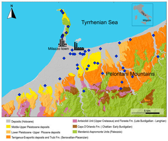
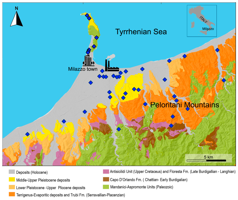
The town of Milazzo (about 29,830 inhabitants) is in the north-eastern part of Sicily (Italy) and extends along the Tyrrhenian coast between latitude 38°13′19.92″ N and longitude 15°14′20.76″ E. It rises over a coastal flat that is 1 m above sea level, with a population density of 1210 inhabitants per square kilometer. Since the 1960s, the industrial area of Milazzo has been characterized by the development of a wide range of industrial facilities, including an oil refinery, thermoelectric power plants, petroleum product storage terminals, and industrial waste landfills. The Milazzo refinery, one of Italy’s major oil processing plants with a capacity exceeding 10 Mt/y, continuously undergoes technological upgrades to enhance efficiency and reduce environmental impact. A substantial share of finished and semi-finished products is shipped by sea from the oil port of Milazzo. The Milazzo district lies within the geological complex known as the “Calabro-Peloritane Arc” (Figure 1). The upper part, known as the “North Peloritani Complex” consists of two main tectonic units: the Aspromonte Unit, characterized by Hercynian amphibolite-facies metamorphic rocks, and the underlying Mandanici Unit, made up of polymetamorphic greenschist-facies rocks [39,40]. Tertiary and Quaternary deposits cover most of the metamorphic sequence [41]. The coastal sector comprises Holocene alluvial deposits, reaching a maximum thickness of 90–100 m in the southern part of the Milazzo Peninsula [42]. According to the Köppen climate classification [43], the study area is categorized as Csa, indicating a Mediterranean climate with dry summers. The wind analysis reveals a regime predominantly influenced by local breeze patterns, originating from West and West-Northwest to South-South-East directions. These data provide valuable insights into the dispersion of atmospheric pollutants in the study area.

Figure 1. Geological map (modified from Gasparo Morticelli et al., [41]) showing sampling locations.

2.2. Biomonitoring Species and Sampling Design

The Mediterranean conifer Pinus pinea L. was selected as the model species for this investigation. These species, thanks to their thin, leathery, needle-like leaves, are highly adapted to the hot, dry summers characteristic of coastal environments, such as the Milazzo district. Pinus pinea L. can grow up to 30 m tall, is highly resinous, usually has a twisted trunk, and features a sparse and irregular crown that is either conical or umbrella-shaped. Its needle-like leaves (6 to 12 cm long) feature a thick waxy cuticle and a complex surface morphology [44], which significantly enhances the interception and long-term accumulation of airborne particulate matter.

A total of 40 pine needle samples were collected during the autumn-winter season of 2023 in the Valle del Mela district. Sampling locations were selected based on the presence of Pinus pinea L. trees, which are randomly distributed across areas near the petrochemical plant, urban areas, and areas far from pollution sources (Figure 1). To ensure a representative evaluation of atmospheric deposition, the sampled P. pinea needles were selected for homogeneity in appearance, age, and crown exposure. Needle sampling was carried out randomly throughout the entire tree crown, from branches not shaded by higher ones, using stainless steel pruning shears. The sampling included green or partially chlorotic needles to obtain a representative sample. The samples were stored in PVC packages and transported to the laboratory.

2.3. Analytical Procedures

The pine needles were placed in an oven at 40 °C for one week to dry. Afterward, they were cut into 5 mm fragments with a surgical scalpel and powdered in an agate mortar.

To minimize sample handling and avoid cross-contamination, each sample was cut using a new, single-use disposable stainless-steel scalpel blade (Swann-Norton, Sheffield, UK), which was replaced after every sample. Although contact time and mechanical abrasion during rapid sectioning were minimized, direct procedural blank validations for the blades were not performed. Therefore, a potential blade-derived bias for Cr and Ni cannot be fully ruled out [45,46,47], and this is acknowledged as a methodological limitation of the sampling protocol.

The chemical analyses were performed at Activation Laboratories Ltd. (Ancaster, ON, Canada). The samples were digested in aqua regia and analyzed by ICP-OES and ICP-MS for Ca, K, Mg, Na, P, Al, As, Ba, Cd, Co, Cr, Cu, Fe, Mn, Mo, Ni, Pb, Sb, Ti, V, Zn, Y, La, Ce, Pr, Nd, Sm, Eu, Gd, Tb, Dy, Ho, Er, Tm, Yb, and Lu. Recovery rates for the certified elements ranged from 96% to 106% when using the standard reference materials CLV-1 (spruce twigs) and CLV-2 (spruce needles). Analytical precision, assessed by duplicate analyses on every tenth sample, ranged from 10% to 16% for all analyzed elements.

A total of 25 pine needle samples, selected based on spatial distribution criteria, were analyzed for their lead isotopic composition (²⁰⁶Pb/²⁰⁷Pb and ²⁰⁸Pb/²⁰⁶Pb ratios). The samples were first subjected to acid digestion using 5 mL of HNO₃. The mineralization process was performed using a Mars X-Press CEM microwave digestion system. The digested samples were sent to the Institut de Physique du Globe de Paris (IPGP), Université Paris Cité, for isotopic analysis.

2.4. Statistical Analysis and Spatial Distribution

Data were analyzed statistically using XLSTAT (2024.1) [48], and all tests were considered statistically significant if p < 0.05. The Shapiro–Wilk test was used to verify the normality of the data distributions. The Spearman correlation matrix was used to measure the association between variables in terms of rank. Factor Analysis (FA) was used to examine relationships among trace elements and identify potential sources of air pollution. The FA model used in this study was applied to elemental raw data. The input variables were the concentrations of 15 selected elements in pine needles. The raw calculated factor loading coefficients were rotated using Kaiser’s varimax rotation scheme [49].

To spatially represent pollutant patterns, we elaborated distribution maps for the same trace element using the program SURFER v. 8.05 (Golden, CO, USA). The maps were based on a grid created by the Kriging interpolation method [50]. The Kriging interpolation models spatial continuity from a finite set of sample points with high inherent variability; therefore, the resulting maps should be interpreted as approximate representations of elemental dispersion across the study area.

2.5. Enrichment Factor Calculation

The Enrichment Factor (EF) was calculated to assess the extent of anthropogenic contamination and to distinguish between crustal and non-crustal sources of trace elements in pine needles. The most widely adopted approach involves normalizing the concentration of a target element against a conservative reference element relative to their respective local background values, which was calculated according to the following equation:

$$EF={\displaystyle \frac{{\left(C_X/C_{\mathrm{Ref}}\right)}_{\mathrm{sample}}}{{\left(C_X/C_{\mathrm{Ref}}\right)}_{\mathrm{baseline}}}}$$

(1)

where $C_X$ represents the concentration of the element of interest, and $C_{\mathrm{Ref}}$ is the concentration of the reference element. The subscripts sample and baseline denote the measured values in the Pinus pinea needles and the regional geogenic baseline for Sicily, respectively [51,52].

While there is no universal consensus on the choice of reference element, it should ideally be geochemically immobile and almost exclusively of crustal origin. Elements such as Al, Fe, Sc, Ti, and Rare Earth Elements (REEs) are the most commonly utilized in environmental studies [53,54,55,56]. Previous studies [54,57] suggest that REEs are preferable reference elements due to their stability and minimal emissions from human activities. In this study, normalization was performed using the total REE concentration (ΣREE), calculated as the sum of La, Ce, Pr, Nd, Sm, Eu, Gd, Tb, Dy, Ho, Er, Tm, Yb, and Lu concentrations.

3. Results and Discussion

The concentrations of the elements studied in needles of Pinus pinea L. are summarized in Table 1.

Table 1. Descriptive statistics of major and trace element concentrations in pine needle samples. D.L.: detection limit, MAD: median absolute deviation, rCV%: robust coefficient of variation. Data are expressed in μg g⁻¹.

		D.L.	Average	Median	Min	Max	MAD	rCV%	Kurtosis	Skewness
Major elements	Ca	25	4466	4280	1090	10,600	980	22	1.8	0.8
	K	10	6881	5910	3510	17,800	1305	19	3.5	1.8
	Mg	2	2885	2870	1220	5000	630	22	−0.1	0.1
	Na	5	4284	2700	175	16,500	1425	33	2.3	1.6
	P	4	1156	965	530	3220	226	20	5.2	2.2
Trace elements	Al	4	156	138.5	72	336	45	29	0.1	0.8
	As	0.01	0.21	0.14	0.05	1.76	0.06	26	22.3	4.4
	Ba	0.1	3.04	2.5	1.0	10.5	0.6	20	7.3	2.5
	Cd	0.006	0.06	0.04	0.01	0.46	0.02	25	16.8	3.8
	Co	0.004	0.13	0.09	0.05	0.85	0.02	15	18.4	4.1
	Cr	0.1	1.0	0.8	0.5	5.30	0.2	21	26.1	4.8
	Cu	0.05	2.92	2.61	1.88	7.51	0.34	12	7.6	2.6
	Fe	3	182	159	85	557	0.04	24	6.7	2.2
	Mn	0.1	37.5	19.4	5.6	295	8.1	21	15.2	3.9
	Mo	0.01	0.46	0.37	0.06	1.35	0.14	31	1.9	1.4
	Ni	0.05	0.86	0.63	0.36	4.79	0.14	16	18.9	3.9
	Pb	0.05	0.63	0.44	0.24	5.52	0.14	21	32.3	5.5
	Sb	0.01	0.11	0.09	0.05	0.66	0.03	26	26.7	4.8
	Ti	0.15	4.26	3.45	1.64	13.2	1.08	25	5.0	2.1
	V	0.01	0.29	0.25	0.11	1.05	0.06	21	9.4	2.9
	Zn	0.4	19.0	16.6	9.1	42.2	3.5	18	1.0	1.3

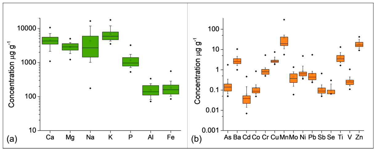
The median concentrations of the macro-elements ranged from 5910 μg g⁻¹ (K) to 138 μg g⁻¹ (Al) with the following order of abundance: K > Ca > Mg > Na > P > Fe > Al. A second group of elements followed the abundance order Mn > Zn > Ti > Cu > Ba > Cr > Ni > Pb > Mo > V > As, with median concentrations ranging from 19 μg g⁻¹ to 0.14 μg g⁻¹. The remaining elements, such as Sb, Co, and Cd, had concentrations below 0.1 μg g⁻¹.

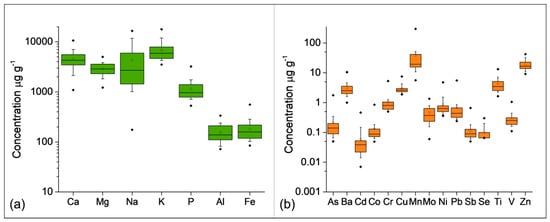
Most of the analyzed elements exhibit non-normal distributions according to the Shapiro–Wilk test (p < 0.05); only Ca and Mg show a normal distribution. The distribution data show considerable variability, with positive skewness and kurtosis for all elements except Mg, which shows negative skewness. Several trace elements, such as As, Cd, Co, Cr, Mn, Mo, Ni, Pb, Sb, V, and Zn, exhibit high kurtosis values above 10, indicating leptokurtic distributions with sharper peaks and heavier tails. Other elements (Ca, Mg, Na, K, P, Al, and Fe) exhibit platykurtic distributions, reflecting flatter peaks and lighter tails. To assess data variability, the robust coefficient of variation (rCV% = MAD/Median × 100) [58] was calculated. In general, a lower %rCV value indicates less relative variation in its concentration. In contrast, higher %rCV values suggest that the median absolute deviation (MAD) exceeds the median, indicating greater variation in element concentrations. The calculated robust coefficient of variation reveals different value ranges: from 0.7% to 20% for elements such as Ba, Co, Cu, K, Ni, P, and Zn; from 20% to 30% for Al, As, Ca, Cd, Cr, Fe, Mg, Mn, Pb, Sb, Ti, and V; and above 30% for Mo and Na, highlighting significant spatial heterogeneity among the sampled sites. The element distributions are shown in Figure 2a,b, underlining the wide variability of major and trace elements.

Figure 2. Boxplots for each element distribution: major (a) and trace elements (b). Whiskers indicate the 10–90% range. The diamond symbols indicate the minimum and maximum values. Data are expressed in μg g⁻¹.

These patterns likely result from heterogeneous environmental inputs, with geogenic and anthropogenic sources contributing to the elemental load in pine needles. Among the detected elements, several are essential nutrients for plant growth, including macronutrients such as Ca, Mg, K, and P, and micronutrients such as Fe, Mn, Zn, and Cu, all of which play a fundamental role in plant metabolic processes. The accumulation of these elements in pine needles therefore reflects not only environmental availability but also physiological uptake and internal regulation mechanisms, making conifer needles an effective biomonitoring matrix for assessing both nutritional status and atmospheric deposition of trace elements [9,10].

In environmental biomonitoring, the analysis of rare-earth element (REE) concentrations provides further insight into the geochemical and environmental processes influencing element accumulation in pine needles. Table 2 reports REE concentrations in pine needle samples. The most abundant lanthanide is Ce, with a median concentration of 143 ng g⁻¹ in pine needles; the other elements follow the following order of abundance, with the lowest value being 0.60 ng g⁻¹ (Tm = Lu) in pine needles: Ce > La > Nd > Y > Pr > Sm > Gd > Dy > Er = Yb > Eu > Ho > Tb > Tm = Lu.

Table 2. Descriptive statistics of REE concentrations in pine needle samples. D.L.: detection limit; MAD: median absolute deviation; rCV%: robust coefficient of variation. Data are expressed in ng g⁻¹.

		D.L.	Average	Median	Min	Max	MAD	rCV%	Kurtosis	Skewness
LREEs	La	10	112	90	50	370	20	18	7.0	2.5
	Ce	15	163	143	66	585	45	27	11.7	2.8
	Pr	1	24	21	10	81	6	25	9.6	2.5
	Nd	5	101	88	41	292	27	27	4.6	1.7
	Sm	1	19	17	6	41	5.0	26	−0.1	0.8
	ΣLREE			359
MREEs	Eu	0.2	3.6	3.3	1.3	9.6	1.0	28	3.7	1.4
	Gd	0.4	16	14	6.8	35.7	4.3	27	0.6	1.0
	Tb	0.2	1.8	1.6	0.6	3.9	0.6	34	0.2	0.7
	ΣMREE			18.9
HREEs	Dy	0.5	12	11.3	4.3	23.4	3.4	29	−0.4	0.6
	Ho	0.2	2.0	1.8	0.6	4	0.6	27	−0.5	0.6
	Er	0.4	5.5	4.8	2.0	11.6	1.6	29	−0.5	0.7
	Tm	0.1	0.8	0.6	0.3	1.6	0.3	33	−0.4	0.8
	Yb	0.4	4.9	4.6	1.4	9.4	1.5	30	−0.5	0.6
	Lu	0.5	0.7	0.6	0.3	1.4	0.3	41	−1.0	0.5
	Y	2	46	43	19	90	15	31	−0.6	0.6
	ΣHREE			66.7
		ΣLREE/ΣHREE		5.4

Classifying rare earth elements into light (LREE), medium (MREE), and heavy (HREE) fractions [59,60] provides a clearer understanding of their biogeochemical pathways. The data reveal a preferential adsorption of LREEs over MREEs and HREEs, as evidenced by a median $\mathsf{\Sigma }\mathrm{LREE}/\mathsf{\Sigma }\mathrm{HREE}$ ratio of 5.4 (Table 2). This fractionation pattern is consistent with observations in other biological and environmental systems [61].

3.1. Multi-Elemental Statistics, Spatial Trends, and Enrichment Factors

Relationships among the elements were investigated using the Spearman correlation matrix (Table 3). A cut-off value of r_s > 0.5 (p < 0.05) was selected to identify statistically robust monotonic relationships, enabling the discrimination of different emission sources. The calculated values were stratified into intensity ranges following the standardized guidelines proposed by Mukaka [62]. The analysis highlights distinct elemental associations, occasionally reflecting multiple contributions to the same element. Chromium exhibited strong correlations (r_s > 0.52) with elements typically associated with industrial and vehicular emissions (Al, Ba, Cu, Fe, Pb, and V).

Table 3. Spearman correlation matrix of variables measured in the pine needle samples. Upper critical value: 0.31 (p < 0.05).

	Al	As	Ba	Cd	Cr	Cu	Fe	Mn	Mo	Ni	Pb	Sb	V	Zn
Al	1.0
As	0.46	1.0							high correlation rs > 0.7
Ba	0.46	0.1	1.0						moderate correlation 0.5 < rs < 0.7
Cd	−0.08	−0.20	0.12	1.0					low correlation 0.31 < rs < 0.5
Cr	0.72	0.33	0.60	−0.05	1.0				negligible correlation rs < 0.31
Cu	0.26	0.08	0.45	0.27	0.50	1.0
Fe	0.82	0.53	0.63	−0.14	0.88	0.50	1.0
Mn	0.19	−0.14	0.26	0.34	0.08	0.05	0.02	1.0
Mo	−0.24	0.09	0.07	−0.13	−0.01	0.41	0.02	0.13	1.0
Ni	0.46	0.05	0.27	0.45	0.48	0.52	0.44	0.41	0.13	1.0
Pb	0.69	0.31	0.55	0.13	0.63	0.23	0.64	0.18	−0.10	0.45	1.0
Sb	0.16	0.21	0.49	−0.16	0.43	0.44	0.51	−0.19	0.31	0.03	0.12	1.0
V	0.62	0.51	0.52	−0.15	0.77	0.44	0.88	−0.11	0.12	0.42	0.57	0.47	1.0
Zn	0.09	−0.19	0.29	0.36	0.29	0.59	0.19	0.31	0.09	0.52	0.25	0.03	0.14	1.0

Copper showed significant correlations with Cr, Ni, and Zn, suggesting a predominantly traffic-related origin. Conversely, Fe showed a strong correlation with Al, likely reflecting a geogenic component associated with the regional metamorphic rocks; however, its robust associations (r_s > 0.60) with Ba, Cr, Pb, and V indicate a mixed origin encompassing both natural and anthropogenic contributions. Lead also displayed a significant correlation with V (r_s = 0.60), further supporting an anthropogenic input linked to the local industrial facilities. The correlation structure provided a solid baseline for the subsequent factor analysis (FA), which identified four main factors explaining a cumulative variance of 75.8% (Table 4). Factor 1 was characterized by high loadings of Fe, As, Na, Al, V, Cr, and Pb. This elemental association points to the influence of multiple sources, including industrial and petrochemical activities, together with the resuspension of crustal material [63]. The co-occurrence of As, Fe, V, and Cr is compatible with emission profiles reported for refinery operations and shipping activities, although additional sources cannot be excluded. Arsenic may also reflect geogenic contributions related to the regional volcanic setting and the local geological background. The presence of Al and Na further suggests the contribution of resuspended soil particles and marine aerosols deposited on needle surfaces [64]. Factor 2 showed strong loadings for Zn, Ni, and Cu, suggesting a possible influence of traffic-related emissions, fuel combustion, and mechanical abrasion processes. Factor 3 was characterized by Ca, Ba, and Mg, consistent with a predominantly geogenic component likely associated with the resuspension carbonate-rich soil dust. Finally, Factor 4 was mainly represented by Sb and Mo, indicating a potential contribution from a combination of urban traffic, port-related activities, and diffuse combustion sources. Antimony is widely recognized as a tracer of non-exhaust vehicular emissions, particularly brake wear particles, which represent a major fraction of traffic-related particulate matter [65,66]. Molybdenum may also be associated with fuel combustion, lubricant oils, and industrial processes [67].

Table 4. Factor loadings (varimax rotation) for pine needle samples.

Principal Component (Marked Loading Are >0.60)	Factor Loadings
	F1	F2	F3	F4
Ca	−0.17	0.03	0.91	0.08
Mg	0.21	−0.20	0.69	−0.11
Na	0.76	−0.23	−0.14	−0.17
Al	0.76	0.34	0.29	−0.20
As	0.79	−0.28	−0.21	0.15
Ba	0.25	0.31	0.75	0.29
Cr	0.69	0.45	0.32	0.19
Cu	0.15	0.68	−0.03	0.58
Fe	0.81	0.32	0.30	0.26
Mo	−0.11	0.06	−0.11	0.76
Ni	0.19	0.82	0.02	0.00
Pb	0.60	0.34	0.48	−0.18
Sb	0.24	−0.03	0.31	0.78
V	0.75	0.28	0.18	0.34
Zn	−0.06	0.83	0.02	0.02
% of variance	27.5	18.1	17.1	13.1

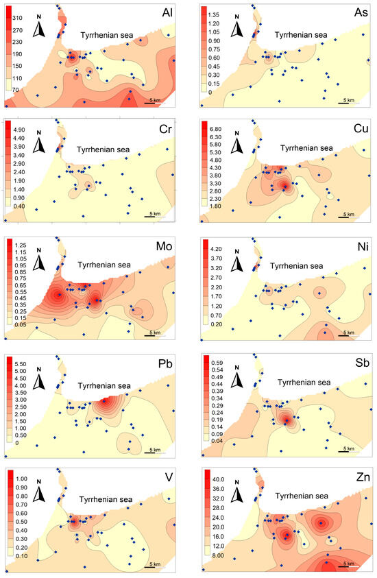
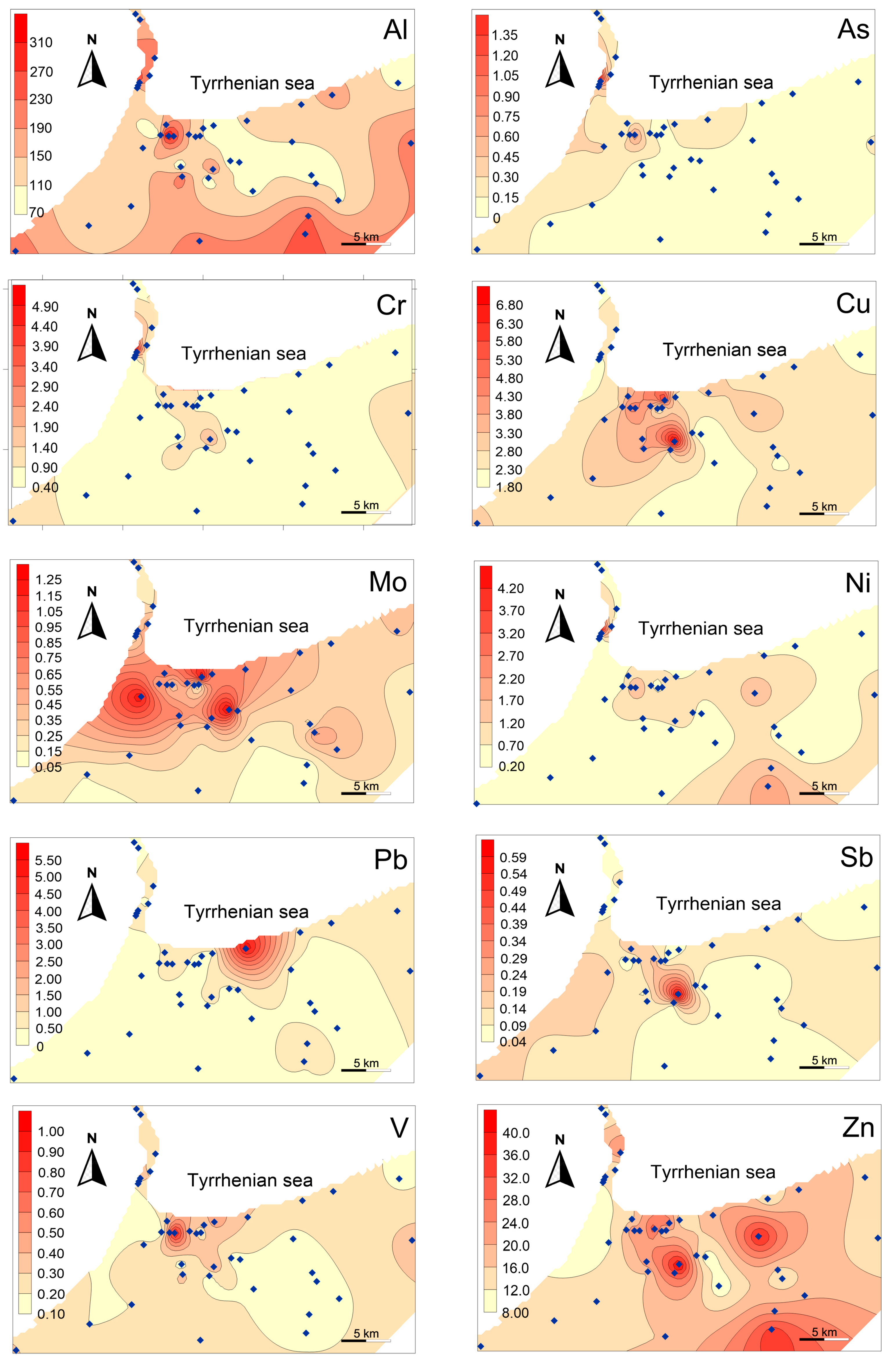
Overall, the FA confirms that pine needles successfully record a complex mixture of environmental contributions. This complexity is further supported by the non-uniform spatial distribution of the elements Al, As, Cr, Cu, Mo, Ni, Pb, Sb, V, and Zn (Figure 3). The distribution maps highlight clear contamination hotspots near the main anthropogenic sources, with dispersion patterns tightly driven by the prevailing wind directions (W-WNW and SSE) toward the hinterland. The areal distribution patterns of Ni, Pb, and V exhibit a distinct industrial signature, with concentrations progressively decreasing farther inland. Molybdenum and antimony levels reflect a dual contribution from both industrial activities and vehicular traffic. In contrast, Cu and Zn display a more heterogeneous pattern, suggesting mixed inputs from urban traffic, industrial emissions, and the geological composition of the local bedrock. For elements such as As, Cr, and Ni, an additional contribution from the Aeolian volcanic arc cannot be ruled out. The absolute concentrations reported for Cr and Ni must be interpreted with appropriate caution, given the potential trace contamination risk during sample sectioning. Nevertheless, because a strictly standardized sectioning protocol was applied uniformly across all samples [45,46,47], the relative spatial patterns and geographical trends observed across the sampling network remain robust and valid for comparative evaluation.

Figure 3. Distribution maps of selected elements in pine needle samples. Data are expressed in μg g⁻¹.

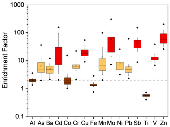
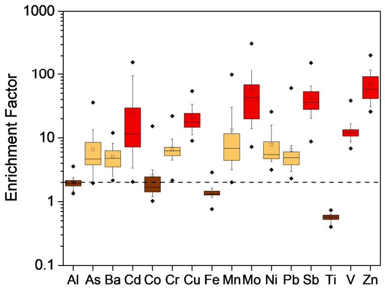
To strictly separate these overlapping geogenic and anthropogenic inputs, the calculated Enrichment Factors (EFs) were evaluated (Figure 4). Following the classification by Hernandez et al. [68], EF values between 0.5 and 2 fall within the range of natural baseline variability, whereas values greater than 2 indicate significant enrichment driven by non-crustal sources. Elements such as Al, Co, Fe, and Ti exhibited EF values between 0.5 and 2, confirming their geogenic origin. Conversely, As, Ba, Cr, Mn, Ni, and Pb had EF values between 2 and 10, revealing a mixed enrichment driven by traffic and industrial activities alongside the weathering of the local metamorphic basement and regional volcanic activity. The highest enrichment (EF > 10) was recorded for Cd, Cu, Mo, Sb, V, and Zn, confirming a dominant anthropogenic fingerprint from local industrial facilities and vehicular traffic. However, for Sb, the influence of the geological background could not be ruled out. For Cu and Zn, the potential influence of the geological context must be considered along with the physiological capacity of pine needles to actively accumulate these elements as essential micronutrients.

Figure 4. Boxplots of enrichment factor (EF) of the analyzed elements in pine needle samples from survey area. The dashed line indicates the boundary between enriched and non-enriched elements.

The normalization of REEs in the calculation of the enrichment factor in biomonitoring needs to take into account the physiological influences on element uptake [61]. In the case of pine needles, their multi-year lifespan and evergreen nature allow for the long-term integration of atmospheric deposition and soil uptake. This structural feature helps smooth out short-term physiological fluctuations and seasonal variations typically observed in annual or herbaceous species. Therefore, the EF values are interpreted by focusing only on clear, large-scale enrichment trends compared to the regional geogenic baseline, avoiding over-interpretation of minor biological variations.

3.2. Lead Isotopic Signatures

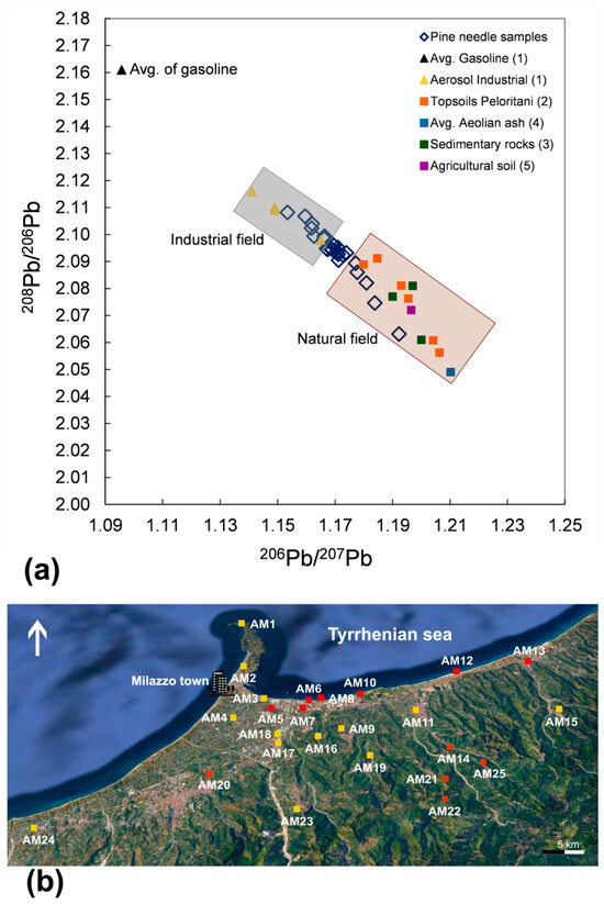
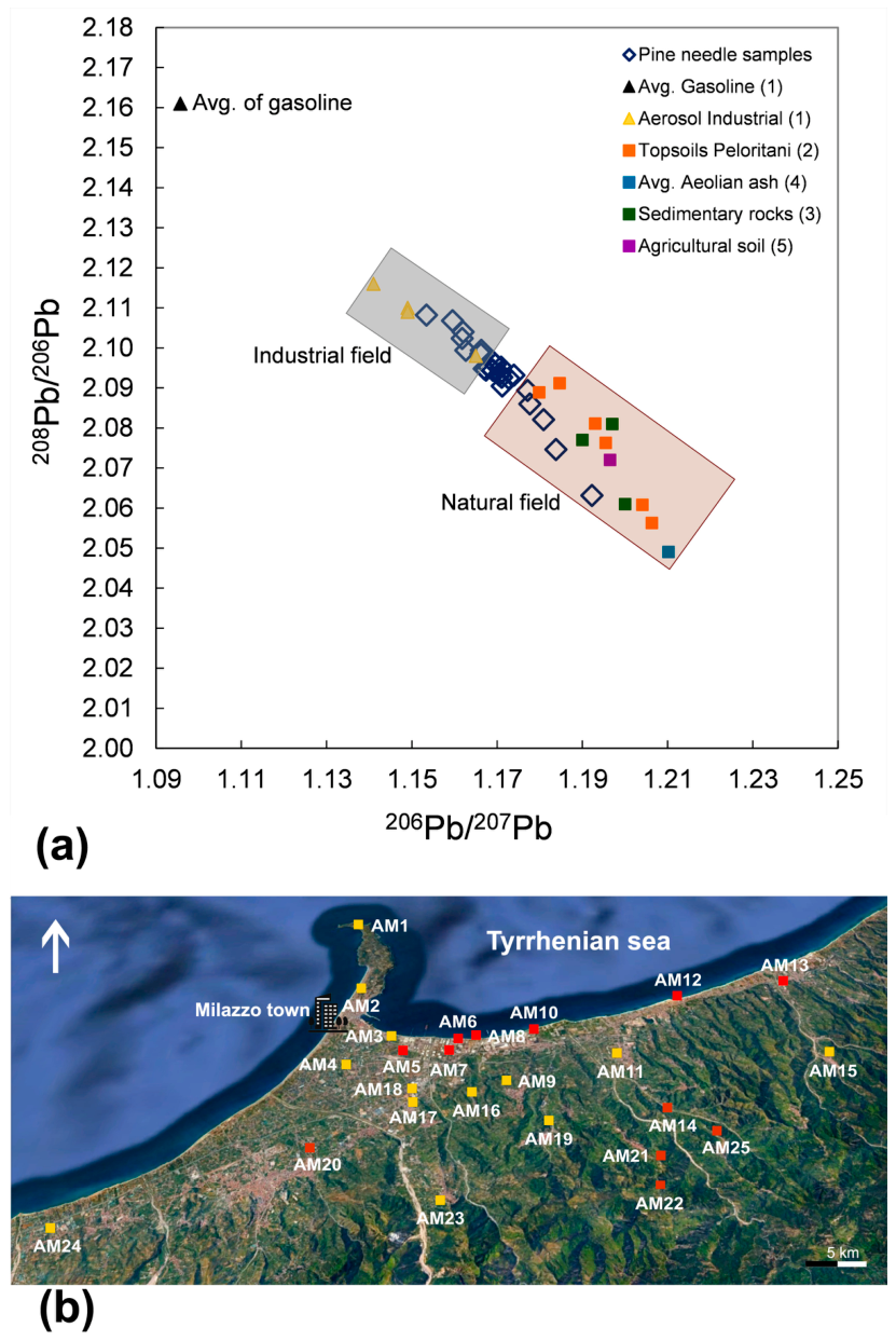
The lead isotopic compositions measured in 25 pine needle samples exhibit a significant dispersion, with ²⁰⁶Pb/²⁰⁷Pb ratios ranging from 1.153 to 1.192 (average: 1.171) and ²⁰⁸Pb/²⁰⁶Pb ratios ranging from 2.063 to 2.108 (average: 2.093) (Table 5). These values deviate markedly from those reported for local rocks (1.190–1.194 for ²⁰⁶Pb/²⁰⁷Pb and 2.076–2.083 for ²⁰⁸Pb/²⁰⁶Pb; [69]), suggesting an anthropogenic influence on the Pb isotopic composition of the pine needles. To accurately constrain the pollution sources, the isotopic data were plotted on a conventional ²⁰⁶Pb/²⁰⁷Pb versus ²⁰⁸Pb/²⁰⁶Pb diagram (Figure 5a). The distribution of samples in isotopic space underscores the complexity of lead sources in the study area. In a previous study, Monna et al. [70] characterized the isotopic composition of lead in gasoline (²⁰⁶Pb/²⁰⁷Pb: 1.066–1.137) and industrial lead (²⁰⁶Pb/²⁰⁷Pb: 1.141–1.165) in Sicily. The isotopic ratios of industrial lead display a range that is considerably more radiogenic than those of gasoline-derived lead.

Table 5. Lead isotopic ratios measured in pine needle samples.

	206Pb/207Pb	208Pb/206Pb
AM1	1.171 ± 0.001	2.093 ± 0.004
AM2	1.174 ± 0.002	2.093 ± 0.003
AM3	1.171 ± 0.002	2.093 ± 0.002
AM4	1.173 ± 0.003	2.092 ± 0.006
AM5	1.166 ± 0.001	2.098 ± 0.003
AM6	1.163 ± 0.001	2.099 ± 0.003
AM7	1.160 ± 0.001	2.107 ± 0.003
AM8	1.162 ± 0.001	2.102 ± 0.003
AM9	1.167 ± 0.003	2.095 ± 0.005
AM10	1.153 ± 0.001	2.108 ± 0.002
AM11	1.169 ± 0.002	2.094 ± 0.003
AM12	1.166 ± 0.002	2.099 ± 0.006
AM13	1.162 ± 0.002	2.104 ± 0.004
AM14	1.181 ± 0.001	2.082 ± 0.005
AM15	1.171 ± 0.002	2.095 ± 0.004
AM16	1.167 ± 0.002	2.094 ± 0.004
AM17	1.171 ± 0.003	2.090 ± 0.005
AM18	1.171 ± 0.002	2.094 ± 0.005
AM19	1.169 ± 0.001	2.097 ± 0.005
AM20	1.177 ± 0.001	2.089 ± 0.003
AM21	1.192 ± 0.002	2.063 ± 0.003
AM22	1.178 ± 0.002	2.086 ± 0.004
AM23	1.170 ± 0.002	2.096 ± 0.005
AM24	1.168 ± 0.003	2.095 ± 0.006
AM25	1.184 ± 0.002	2.075 ± 0.004

Figure 5. (a) Lead stable isotope ratios (²⁰⁸Pb/²⁰⁶Pb vs. ²⁰⁶Pb/²⁰⁷Pb) in pine needle samples. The compositional fields of natural and anthropogenic lead sources are also plotted for comparative purposes. 1 (Monna et al., [70]), 2 (Cosenza et al., [69]), 3 (Alaimo et al., [23]), 4 (Schiavi et al., [71]); 5 (Reiman et al., [72]). (b) The sampling points for the three groups. Group I (red): industrial; Group II (yellow): transitional/mixing zone; Group III (brown): geogenic.

In our dataset, the samples plot far away from the old leaded gasoline field, confirming that past contamination plays a negligible role, whereas active industrial emissions dominate the current anthropogenic input. The spatial and isotopic distribution reveals a non-uniform pattern, defining a distinct three-component mixing trend controlled by topography and local wind regimes (Figure 5b).

Group I (industrial) is located in the coastal lowlands near the Milazzo refinery and thermoelectric complex. These samples display the lowest ²⁰⁶Pb/²⁰⁷Pb ratios (1.153–1.165), closely matching the signatures of industrial fuel oil combustion and petrochemical processing. Group II (transitional/mixing zone) is spatially distributed across the study area. This group defines a clear binary mixing line stretching between the industrial endmember and the local crustal background. The intermediate isotopic ratios reflect the progressive atmospheric dilution of industrial particulate matter as it is transported inland by the prevailing W-WNW and SSE breezes. Group III (geogenic) is situated at higher altitudes along the Peloritani ridge. These samples tightly cluster within the natural geogenic field of local rocks (²⁰⁶Pb/²⁰⁷Pb ~ 1.190). However, the slight horizontal shift in some high-altitude samples suggests a subtle, overlapping contribution from the active Aeolian volcanic arc (e.g., Stromboli and Vulcano emissions, typically characterized by high ²⁰⁸Pb/²⁰⁶Pb fluxes). Overall, the relative position of the samples along the isotopic trend provides a semi-quantitative indication of the contribution of the different Pb sources. Samples located close to the industrial end-member are interpreted as reflecting a predominant anthropogenic contribution, whereas samples progressively approaching the local crustal signature indicate increasing influence of natural background Pb. The isotopic gradient clearly supports a decreasing influence of industrial emissions with increasing distance and elevation from the main emission areas.

4. Conclusions

This study demonstrates that Pinus pinea L. needles represents an efficient biomonitoring tool for assessing atmospheric trace-element deposition and characterizing spatial variability in complex industrial areas. By integrating multi-elemental analysis, geostatistical mapping, and lead isotopic fingerprints, this approach disentangled overlapping natural and anthropogenic inputs in the heavily industrialized Milazzo district.

The main findings confirm a persistent environmental pressure heavily driven by local industrial activities, particularly around the refinery, industrial plants, urbanized areas, and port-related activities. Major lithogenic elements such as Al, Fe, and Ti reflect the local geogenic composition, while trace elements like As, Cr, Mo, Ni, Pb, Sb, V, and Zn exhibit clear anthropogenic enrichment. The combination of multivariate statistics with Pb isotopic tracking indicated that atmospheric pollution in the area is not uniform but arises from a complex, multi-source network in which petrochemical emissions, non-exhaust vehicular traffic, and marine and volcanic inputs continuously overlap under the control of local wind regimes.

From an environmental health and management perspective, these results provide valuable site-specific insights into the distribution and potential sources of atmospheric trace elements in a high-risk area (Milazzo SIN). The spatial resolution achieved through pine needle sampling can support local authorities in designing targeted air-quality mitigation strategies, optimizing institutional monitoring networks, and refining future environmental risk assessment programs in industrialized Mediterranean coastal zones. Finally, future biomonitoring studies targeting metal and metalloid analyses could further refine sample preparation procedures by selecting inert tools to eliminate any potential background noise. Crucially, the choice of inert tool must be strictly tailored to the target elements being quantified, ensuring that the equipment material does not introduce impurities that interfere with the detection of the specific analytes of interest.

References

- Ali, H.; Khan, E.; Ilahi, I. Environmental chemistry and ecotoxicology of hazardous heavy metals: Environmental persistence, toxicity, and bioaccumulation. J. Chem. 2019, 2019, 6730305. [Google Scholar] [CrossRef] [Scilit]
- Garrett, R.G. Natural sources of metals to the environment. GEEA 2010, 10, 99–110. [Google Scholar]
- Briffa, J.; Sinagra, E.; Blundell, R. Heavy metal pollution in the environment and their toxicological effects on humans. Heliyon 2020, 6, e04691. [Google Scholar] [CrossRef] [Scilit] [PubMed]
- Nriagu, J.O.; Pacyna, J.M. Quantitative assessment of worldwide contamination of Air, Water and Soils by Trace Metals. Nature 1988, 333, 134–139. [Google Scholar] [CrossRef] [Scilit] [PubMed]
- Pacyna, J.M.; Scholtz, T.; Li, Y.-F. Global budget of trace metals sources. Environ. Rev. 1995, 3, 145–159. [Google Scholar] [CrossRef] [Scilit]
- Gałuszka, A.; Migaszewski, Z.M. Geochemical background-an environmental perspective. Mineralogia 2011, 42, 7–17. [Google Scholar] [CrossRef] [Scilit]
- Kicińska, A.; Turek, K. Establishing geochemical background of elements present in soil and its application in the evaluation of soil pollution based on data collected in the Beskid Sądecki region. Geoinf. Pol. 2017, 16, 87–99. [Google Scholar] [CrossRef] [Scilit]
- Markert, B. Plants as Biomonitors: Indicators for Heavy Metals in the Terrestrial Environment; VCH: Weinheim, Germany, 1993. [Google Scholar]
- Bargagli, R. Trace Elements in Terrestrial Plants. An Ecophysiological Approach to Biomonitoring and Biorecovery; Springer: Berlin/Heidelberg, Germany, 1998. [Google Scholar]
- Markert, B.; Breure, A.M.; Zechmeister, H.G. Bioindicators and biomonitors: Principles, concepts, and applications. In Trace Metals and Other Contaminants in the Environment; Elsevier: Amsterdam, The Netherlands, 2003; Volume 6, pp. 15–25. [Google Scholar]
- Cavazzin, B.; MacDonell, C.; Green, N.; Rothwell, J.J. Air pollution biomonitoring in an urban-industrial setting (Taranto, Italy) using Mediterranean plant species. Atmos. Pollut. Res. 2024, 15, 102105. [Google Scholar] [CrossRef] [Scilit]
- Beckett, K.P.; Freer-Smith, P.; Taylor, G. Effective tree species for local air-quality management. Arboric. Urban For. 2000, 26, 12–19. [Google Scholar] [CrossRef] [Scilit]
- Lehndorff, E.; Schwark, L. Biomonitoring of air quality in the Cologne Conurbation using pine needles as a passive sampler—Part III: Major and trace elements. Atmos. Environ. 2010, 44, 2822–2829. [Google Scholar] [CrossRef] [Scilit]
- Wolterbeek, B. Biomonitoring of trace element air pollution: Principles, possibilities and perspectives. Environ. Pollut. 2002, 120, 11–21. [Google Scholar] [CrossRef] [Scilit] [PubMed]
- Szczepaniak, K.; Biziuk, M. Aspects of the biomonitoring studies using mosses and lichens as indicators of metal pollution. Environ. Res. 2003, 93, 221–230. [Google Scholar] [CrossRef] [Scilit] [PubMed]
- Santitoro, A.; Aprile, G.G.; Baldantoni, D.; Bartoli, G.; Alfani, A. Trace element analyses in an epiphytic lichen and its bark substrate to assess suitability for air biomonitoring. Environ. Monit. Assess. 2004, 98, 59–67. [Google Scholar] [CrossRef] [Scilit] [PubMed]
- Sawidis, T.; Breuste, J.; Mitrovic, M.; Pavlovic, P.; Tsigaridas, K. Trees as bioindicator of heavy metal pollution in three European cities. Environ. Pollut. 2011, 159, 3560–3570. [Google Scholar] [CrossRef] [Scilit] [PubMed]
- Garty, J. Biomonitoring atmospheric heavy metals with lichens: Theory and application. Crit. Rev. Plant Sci. 2001, 20, 309–371. [Google Scholar] [CrossRef] [Scilit]
- Steinnes, E. Use of mosses to study atmospheric deposition of trace elements: Contributions from investigations in Norway. Int. J. Environ. Pollut. 2008, 32, 499–508. [Google Scholar] [CrossRef] [Scilit]
- Bargagli, R. Moss and lichen biomonitoring of atmospheric mercury: A review. Sci. Total Environ. 2016, 572, 216–231. [Google Scholar] [CrossRef] [Scilit] [PubMed]
- Aničić, M.; Spasić, T.; Tomašević, M.; Rajšić, S.; Tasić, M. Trace elements accumulation and temporal trends in leaves of urban deciduous trees (Aesculus hippocastanum and Tilia spp.). Ecol. Indic. 2011, 11, 824–830. [Google Scholar]
- Sgrigna, G.; Sæbø, A.; Gawronski, S.; Popek, R.; Calfapietra, C. Particulate Matter deposition on Quercus ilex leaves in an industrial city of central Italy. Environ. Pollut. 2015, 197, 187–194. [Google Scholar] [CrossRef] [Scilit] [PubMed]
- Alaimo, M.G.; Dongarrà, G.; Melati, M.R.; Monna, F.; Varrica, D. Recognition of environmental trace metal contamination using pine needles as bioindicators. The urban area of Palermo (Italy). Environ. Geol. 2000, 39, 914–924. [Google Scholar] [CrossRef] [Scilit]
- Bertolotti, G.; Gialanella, S. Review: Use of conifer needles as passive samplers of inorganic pollutants in air quality monitoring. Anal. Methods 2014, 6, 6208–6222. [Google Scholar] [CrossRef] [Scilit]
- Abbaszade, G.; Tserendorj, D.; Salazar-Yanez, N.; Zacháry, D.; Völgyesi, P.; Tóth, E.; Szabó, C. Lead and stable lead isotopes as tracers of soil pollution and human health risk assessment in former industrial cities of Hungary. Appl. Geochem. 2022, 145, 105397. [Google Scholar] [CrossRef] [Scilit]
- Komárek, M.; Ettler, V.; Chrastný, V.; Mihaljevič, M. Lead isotopes in environmental sciences: A review. Environ. Int. 2008, 34, 562–577. [Google Scholar] [CrossRef] [Scilit] [PubMed]
- Shotyk, W.; Weiss, D.; Appleby, P.G.; Cheburkin, A.K.; Frei, R.; Gloor, M.; Kramers, J.D.; Reese, S.; Van Der Knaap, W.O. History of Atmospheric Lead Deposition Since 12,370 14C yr BP from a Peat Bog, Jura Mountains. Science 1998, 281, 1635–1640. [Google Scholar] [CrossRef] [Scilit] [PubMed]
- Reimann, C.; Fabian, K.; Flem, B.; Schilling, J.; Roberts, D.; Englmaier, P. Pb concentrations and isotope ratios of soil O and C horizons in Nord-Trøndelag, central Norway: Anthropogenic or natural sources? Appl. Geochem. 2016, 74, 56–66. [Google Scholar] [CrossRef] [Scilit]
- Sensuła, B.; Fagel, N.; Michczyński, A. Radiocarbon, trace elements and Pb isotope composition of pine needles from a highly industrialized region in southern Poland. Radiocarbon 2021, 63, 713–726. [Google Scholar] [CrossRef] [Scilit]
- Varrica, D.; Dongarrà, G.; Alaimo, M.G.; Monna, F.; Losno, R.; Sanna, E.; De Giudici, G.; Tamburo, E. Lead isotopic fingerprint in human scalp hair: The case study of Iglesias mining district (Sardinia, Italy). Sci. Total Environ. 2018, 613–614, 456–461. [Google Scholar] [CrossRef] [Scilit] [PubMed]
- Bollhöfer, A.; Rosman, K.J.R. Isotopic source signatures for atmospheric lead: The Southern Hemisphere. Geoch. Cosm. Act. 2000, 64, 3251–3262. [Google Scholar] [CrossRef] [Scilit]
- Veysseyre, A.M.; Bollhöfer, A.F.; Rosman, K.J.R.; Ferrari, C.P.; Boutron, C.F. Tracing the Origin of Pollution in French Alpine Snow and Aerosols Using Lead Isotopic Ratios. Environ. Sci. Technol. 2001, 35, 4463–4469. [Google Scholar] [CrossRef] [Scilit] [PubMed]
- Liu, J.; Bi, X.; Li, F.; Wang, P.; Wu, J. Source discrimination of atmospheric metal deposition by multi-metal isotopes in the Three Gorges Reservoir region, China. Environ. Pollut. 2018, 240, 582–589. [Google Scholar] [CrossRef] [Scilit] [PubMed]
- Chen, Y.; Ning, Y.; Bi, X.; Liu, J.; Yang, S.; Liu, Z.; Huang, W. Pine needles as urban atmospheric pollution indicators: Heavy metal concentrations and Pb isotopic source identification. Chemosphere 2022, 296, 134043. [Google Scholar] [CrossRef] [Scilit] [PubMed]
- Pirastu, R.; Ancona, C.; Iavarone, I.; Mitis, F.; Zona, A.; Comba, P. SENTIERI Project Mortality study of residents in Italian polluted sites: Evaluation of the epidemiological evidence. Epidemiol. Prev. 2010, 34, 4–96. [Google Scholar]
- Dongarrà, G.; Ottonello, D.; Sabatino, G.; Triscari, M. Use of lichens in detecting environmental risk and in geochemical prospecting. Environ. Geol. 1995, 26, 139–146. [Google Scholar] [CrossRef] [Scilit]
- Triolo, L.; Binazzi, A.; Cagnetti, P.; Carconi, P.; Correnti, A.; De Luca, E.; Di Bonito, R.; Grandoni, G.; Mastrantonio, M.; Rosa, S.; et al. Air pollution impact assessment on agroecosystem and human health characterisation in the area surrounding the industrial settlement of Milazzo (Italy): A multidisciplinary approach. Environ. Monit. Assess. 2008, 140, 191–209. [Google Scholar] [CrossRef] [Scilit] [PubMed]
- Cangemi, M.; Madonia, P.; Albano, L.; Bonfardeci, A.; Di Figlia, M.G.; Di Martino, R.M.R.; Nicolosi, M.; Favara, R. Heavy Metal Concentrations in the Groundwater of the Barcellona-Milazzo Plain (Italy): Contributions from Geogenic and Anthropogenic Sources. Int. J. Environ. Res. Public Health 2019, 16, 285. [Google Scholar] [CrossRef] [Scilit] [PubMed]
- Ferla, P. A model of continental crust evolution in the geological history of the Peloritani Mountains (Sicily). Mem. Soc. Geol. Ital. 2000, 55, 87–93. [Google Scholar]
- Punturo, R.; Kern, H.; Cirrincione, R.; Mazzoleni, P.; Pezzino, A. P- and S-wave velocities and densities in silicate and calcite rocks from the Peloritani Mountains, Sicily (Italy): The effect of pressure, temperature and the direction of wave propagation. Tectonophysics 2005, 409, 55–72. [Google Scholar] [CrossRef] [Scilit]
- Gasparo Morticelli, M.; Valenti, V.; Catalano, R.; Sulli, A.; Agate, M.; Avellone, G.; Albanese, C.; Basilone, L.; Gugliotta, C. Deep controls on foreland basin system evolution along the Sicilian fold and thrust belt. Bull. Soc. Géol. Fr. 2015, 186, 273–290. [Google Scholar] [CrossRef] [Scilit]
- Carbone, S.; Messina, A.; Lentini, F.; Macaione, E. CARG—CARtografia Geologica di Italia-Note Illustrative Della Carta Geologica d’Italia, Fogli 587 e 600 (Milazzo-Barcellona P.G.); Servizio Geologico d’Italia: Rome, Italy, 2011. [Google Scholar]
- Kottek, M.; Grieser, J.; Beck, C.; Rudolf, B.; Rubel, F. World Map of the Köppen-Geiger climate classification updated. Meteorol. Z. 2006, 15, 259–263. [Google Scholar] [CrossRef] [Scilit] [PubMed]
- Ferrari, M.; Medici, D. Alberi e Arbusti in Italia; Edagricole: Bologna, Italy, 1996. [Google Scholar]
- Bich, L.; My, H.; Dinh, R.; Minh, T.; Trong, T.; Harper, S.; Wuhrer, R.; Huang, Q.; George, L.; Holford, P.; et al. Trace Metal Contamination During Grinding of Plant Samples. Commun. Soil Sci. Plant Anal. 2018, 50, 102–107. [Google Scholar] [CrossRef] [Scilit]
- Versieck, J.; Cornelis, R. Normal levels of trace elements in human blood plasma or serum. Anal. Chim. Acta 1980, 116, 217–254. [Google Scholar] [CrossRef] [Scilit]
- Allan, A.M.; Blakeney, A.B.; Batten, G.D.; Dunn, T.S. Impact of grinder configurations on grinding rate, particle size, and trace element contamination of plant samples. Commun. Soil Sci. Plant Anal. 1999, 30, 2123–2135. [Google Scholar] [CrossRef] [Scilit]
- Lumivero XLSTAT Statistical and Data Analysis Solution; Lumivero: Denver, CO, USA, 2024.
- Kaiser, H.F. The varimax criteria for analytical rotation in factor analysis. Psychometrika 1958, 23, 187–200. [Google Scholar] [CrossRef] [Scilit]
- Cressie, N.A.C. Statistics for Spatial Data; John Wiley and Sons, Inc.: New York, NY, USA, 1991. [Google Scholar]
- Lo Medico, F.; Varrica, D.; Zuccolini, M.V.; Miola, M.; Scopelliti, G.; Alaimo, M.G. Geochemical baseline values and spatial distribution of major, trace, and rare earth elements in unpolluted soils of the Sicily region (Italy). Environ. Geochem. Health 2025, 47, 167. [Google Scholar] [CrossRef] [Scilit] [PubMed]
- Varrica, D.; Lo Medico, F.; Zuccolini, M.V.; Miola, M.; Alaimo, M.G. Geochemical baseline values determination and spatial distribution of trace elements in topsoils: An application in Sicily region (Italy). Sci. Total Environ. 2024, 955, 176951. [Google Scholar] [CrossRef] [Scilit] [PubMed]
- Yongming, H.; Peixuan, D.; Junji, C.; Posmentier, E.S. Multivariate analysis of heavy metal contamination in urban dusts of Xi’an, Central China. Sci. Tot. Environ. 2006, 355, 176–186. [Google Scholar] [CrossRef] [Scilit] [PubMed]
- Lehndorff, E.; Schwark, L. Accumulation histories of major and trace elements on pine needles in the Cologne Conurbation as function of air quality. Atmos. Environ. 2008, 42, 833–845. [Google Scholar] [CrossRef] [Scilit]
- Sardans, J.; Peñuelas, J. Introduction of the Factor of Partitioning in the Lithogenic Enrichment Factors of Trace Element Bioaccumulation in Plant Tissues. Environ. Monit. Assess. 2006, 115, 473–498. [Google Scholar] [CrossRef] [Scilit] [PubMed]
- Tyler, G. Rare earth elements in soil and plant systems—A review. Plant Soil 2004, 267, 191–206. [Google Scholar] [CrossRef] [Scilit]
- Wyttenbach, A.; Furrer, V.; Schleppi, P.; Tobler, L. Rare earth elements in soil and in soil-grown plants. Plant Soil 1998, 199, 267–273. [Google Scholar] [CrossRef] [Scilit]
- Ambrosino, M.; Palarea-Albaladejo, J.; Albanese, S.; Lin, X.; Ciarcia, S.; Cicchella, D. Assessing natural background concentrations of chemical elements in urban soils: A case study in Benevento (Italy). Sci. Total Environ. 2025, 975, 179298. [Google Scholar] [CrossRef] [Scilit] [PubMed]
- Chen, J.; Algeo, T.J.; Zhao, L.; Chen, Z.-Q.; Cao, L.; Zhang, L.; Li, Y. Diagenetic uptake of rare earth elements by bioapatite, with an example from Lower Triassic conodonts of South China. Earth Sci. Rev. 2015, 149, 181–202. [Google Scholar] [CrossRef] [Scilit]
- Dubinin, A.V. Geochemistry of Rare Earth Elements in the Ocean. Lithol. Miner. Resour. 2004, 39, 289–307. [Google Scholar] [CrossRef] [Scilit]
- Brioschi, L.; Steinmann, M.; Lucot, E.; Pierret, M.C.; Stille, P.; Prunier, J.; Badot, P.M. Transfer of rare earth elements (REE) from natural soil to plant systems: Implications for the environmental availability of anthropogenic REE. Plant Soil 2013, 366, 143–163. [Google Scholar] [CrossRef] [Scilit]
- Mukaka, M.M. Statistics corner: A guide to appropriate use of correlation coefficient in medical research. Malawi Med. J. 2012, 24, 69–71. [Google Scholar] [PubMed]
- Suvarapu, L.N.; Baek, S.O. Determination of heavy metals in the ambient atmosphere. Toxicol. Ind. Health 2017, 33, 79–96. [Google Scholar] [CrossRef] [Scilit] [PubMed]
- Juranović Cindrić, I.; Zeiner, M.; Starčević, A.; Stingeder, G. Metals in pine needles: Characterisation of bio-indicators depending on species. Int. J. Environ. Sci. Technol. 2019, 16, 4339–4346. [Google Scholar] [CrossRef] [Scilit]
- Feo, M.L.; Torre, M.; Tratzi, P.; Battistelli, F.; Tomassetti, L.; Petracchini, F.; Guerriero, E.; Paolini, V. Laboratory and on-road testing for brake wear particle emissions: A review. Environ. Sci. Pollut. Res. 2023, 30, 100282–100300. [Google Scholar] [CrossRef] [Scilit] [PubMed]
- Pleijel, H.; Klingberg, J.; Strandberg, B.; Sjöman, H.; Wallin, G. Accumulation of antimony and lead in leaves and needles of trees: The role of traffic emissions. Heliyon 2023, 8, 13548. [Google Scholar] [CrossRef] [Scilit] [PubMed]
- Bosco, M.L.; Varrica, D.; Dongarrà, G. Case Study: Inorganic pollutants associated with particulate matter from an area near a petrochemical plant. Environ. Res. 2005, 99, 18–30. [Google Scholar] [CrossRef] [Scilit] [PubMed]
- Hernandez, L.; Probst, A.; Probst, J.L.; Ulrich, E. Heavy metal distribution in some French forest soils: Evidence for atmospheric contamination. Sci. Total Environ. 2003, 312, 195–219. [Google Scholar] [CrossRef] [Scilit] [PubMed]
- Cosenza, A.; Lima, A.; Ayuso, R.A.; Foley, N.K.; Albanese, S.; Messina, A.; De Vivo, B. Soil geochemical survey of abandoned mining sites in the Eastern-Central Peloritani Mountains, Sicily, Italy. GEEA 2015, 15, 361–372. [Google Scholar] [CrossRef] [Scilit]
- Monna, F.; Aiuppa, A.; Varrica, D.; Dongarra, G. Pb Isotope Composition in Lichens and Aerosols from Eastern Sicily: Insights into the Regional Impact of Volcanoes on the Environment. Environ. Sci. Technol. 1999, 33, 2517–2523. [Google Scholar] [CrossRef] [Scilit]
- Schiavi, F.; Kobayashi, K.; Nakamura, E.; Tiepolo, M.; Vannucci, R. Trace element and Pb–B–Li isotope systematics of olivine-hosted melt inclusions: Insights into source metasomatism beneath Stromboli (southern Italy). Contrib. Mineral. Petrol. 2012, 163, 1011–1031. [Google Scholar] [CrossRef] [Scilit]
- Reimann, C.; Flem, B.; Fabian, K.; Birke, M.; Ladenberger, A.; Négrel, P.; Demetriades, A.; Hoogewerff, J. Lead and lead isotopes in agricultural soils of Europe-the continental perspective. Appl. Geochem. 2012, 27, 532–542. [Google Scholar] [CrossRef] [Scilit]
Disclaimer/Publisher’s Note: The statements, opinions and data contained in all publications are solely those of the individual author(s) and contributor(s) and not of MDPI and/or the editor(s). MDPI and/or the editor(s) disclaim responsibility for any injury to people or property resulting from any ideas, methods, instructions or products referred to in the content. |
© 2026 by the authors. Licensee MDPI, Basel, Switzerland. This article is an open access article distributed under the terms and conditions of the Creative Commons Attribution (CC BY) license.