


Abstract
This study explores the potential of Artificial Neural Networks (ANNs) for the calculation of momentum and sensible heat fluxes. The ANN is applied on idealized Large Eddy Simulation (LES) data. The LES test cases used to train the ANN correspond to convective conditions with partially low wind speeds and heterogeneous surfaces. To enable the ANN to learn the systematics of such conditions, the input variables for the ANN include the variables that are used in Monin Obukhov Similarity Theory (MOST) and an additional variable that accounts for the heterogeneity of the land surface. Simulation data is averaged over 30 min and different spatial scales. Our findings show that the modeling skill is generally higher for momentum flux than for sensible heat flux. Also, the performance increases with larger spatial-averaging scales. The ANN calculates momentum flux with a correlation of 0.81 and a normalized RMSE of 0.59 for a single grid point. On a spatial-averaging scale of 4000 m, the correlation changes to almost 1.00 and the normalized RMSE to 0.05. The importance of each input variable for model performance is determined with a feature importance weighting. Their relative importance depends strongly on the spatial-averaging scale. The importance of the variable that represents the influence of surface heterogeneity is low at smaller spatial-averaging scales, but increases at larger averaging scales. However, its contribution to the modeling skill is small. Reducing the number of input variables to two results in a substantial loss of performance. Although our results demonstrate the potential of this approach to improve the calculation of momentum and sensible heat fluxes, it is also clear that there are simplifications and limitations in the present setup that need to be overcome to assess general applicability. These include the height of analysis (40 m instead of 10 m or less), the exclusion of all latent heat processes, the exclusion of stable conditions, the data coverage of the required parameter space, and the usage of only surface roughness length to define surface heterogeneity.
1. Introduction
The surface fluxes determine the distribution of energy between the Earth’s surface and the atmosphere. According to the concept of surface energy balance, the Sun’s irradiation is partially absorbed at the surface and transformed into heat, driving the ground heat flux, latent heat flux, and sensible heat flux. These fluxes shape the vertical profiles of wind, temperature, and humidity, which has implications on the local state of the atmosphere as well as the large-scale circulation. Hence, simulations of the atmosphere require a representation of momentum flux (MF) and sensible heat flux (HF).
MF and HF in the surface layer take place via turbulent processes. The generation of turbulence can be induced mechanically (by wind shear) or thermally (by buoyancy) [1]. Weather and climate models have a horizontal resolution on the scale of kilometers, which is larger than most of the relevant turbulent processes. MF and HF are therefore being parameterized in such models. Monin Obukhov Similarity Theory (MOST) is commonly used as a parameterization method [2]. It relates the magnitude of the turbulent fluxes to the gradients of the respective quantities. This relationship is dependent on a dimensionless stability parameter. However, MOST relies on simplified assumptions. Strictly speaking, it is only valid for smooth and homogeneous surfaces with windy, stationary, and near-neutral conditions. This is often not met in reality, with poor performance of MOST under deviating conditions [3,4]. Despite these shortcomings, MOST is still commonly used.
One focus of this study is to account for the effect of land surface heterogeneity, as it is known to influence atmospheric circulation [5,6]. Batches of heterogeneous land surface differ in several physical properties, such as surface roughness length, albedo, evaporation, and transpiration. This causes differences in shear stress, heat generation, and transport, and consequently modulates the values of MF and HF [7,8]. The scales of heterogeneity reach well below the resolution of mesoscale models, which is why mesoscale models commonly incorporate subgrid scale heterogeneity via flux aggregation techniques [9].
Large Eddy Simulations (LESs) simulate the atmosphere in limited domains with a high resolution. In this study, we explore the potential of Artificial Neural Networks (ANNs) to reproduce the values of MF and HF that are obtained in a LES, especially in conditions in which MOST is not performing well. The LES acts as an ‘observation system experiment’, as we use the output of the LES to train and test the ANN. The simulations are set up in unstable conditions, and the domains include idealized heterogeneity features. While the LES also uses MOST to parameterize the turbulent fluxes at the lower boundary, a vast part of the turbulent spectrum is calculated explicitly in the model layers above. The fluxes and variables in these model layers can therefore be treated as robust data [10]. All input and target variables for the ANN are given and available in 3D in the experiment domains. This is an advantage over real-world observations that allow only a limited data coverage in space and time. By examining the performance of the ANN, we hope to gain knowledge of the potential of this approach to improve turbulent flux parameterizations in mesoscale models over heterogeneous terrain.
Several studies have investigated the capability of employing ANNs to calculate turbulent fluxes in the boundary layer. Ref. [11] investigated the potential of ANNs to calculate turbulent fluxes and compared the accuracy and computation time to MOST, using measurement data. MOST and ANNs performed similarly good. Ref. [4] trained an ANN on tower measurement data and compared the results to MOST, Bulk Richardson similarity, and Extreme Gradient Boosting, another machine learning technique. The machine learning methods outperformed the conventional methods. In a detailed study, ref. [12] trained an ANN on tower data and applied it in an LES model both offline and online. Furthermore, they used LES output to account for values of surface roughness and height above ground that deviate from those in the training data. Ref. [13] use a Random Forest machine learning model trained with idealized LES data to calculate dispersive fluxes and reduce the surface energy balance gap in both LES simulations and field measurements.
In contrast to the aforementioned studies, our focus is on using idealized LES data for training and validation and using only data that would be accessible for a mesoscale model. In addition, the influence of spatial-averaging on the modeling performance of MF and HF is investigated, similarly to [14] who examined the modeling skill of MOST for HF depending on the spatial-averaging scale.
The benefit of all input variables, in particular those using information on land surface characteristics, is examined via a Feature Importance Weighting (FIW). Furthermore, based on the results of the FIW, an ANN as well as a polynomial regression are applied with a reduced number of input variables and evaluated. Polynomial regression is a common method to approximate values of a target variable based on one or more input variables and used for example by [15] to model the dissipation of turbulent kinetic energy.
The questions to be answered in this study are the following: How well can an ANN reproduce MF and HF calculated by an LES and what is the influence of spatial averaging? What are the problems this approach would have to overcome to develop a parameterization for mesoscale models? What is the benefit of using surface heterogeneity information when modeling MF and HF?
2. Materials and Methods
2.1. Flux Calculation
2.1.1. Artificial Neural Networks
An Artificial Neural Network (ANN) is a tool that predicts the values of target variables based on the values of input variables [16]. A Multilayer Perceptron (MLP) is a fully connected, feed-forward ANN with one or several hidden layers of artificial neurons [17]. It propagates the input with a weight to the next layers and finally the output neuron. The MLP is trained with datasets that contain input data and the corresponding true output. During training, it minimizes a loss function by adjusting the weights to reduce the error of the output variable. It can therefore find relations of any nature between input and target variables. This enables the MLP to make predictions based on input variables and their relationships learned in the training process.
In this case, the input variables are potential temperature , horizontal wind speed , their respective difference with height and , and the mean and variance of the surface roughness length ( mean and variance) in the corresponding spatial area. These quantities are chosen because they are believed to be related to MF and HF and because they could be accessed similarly by a large-scale model in the calculation process. That means that the prognostic variables of temperature and wind are only used as spatial means of the area in which the output variables are calculated. In a further step, only a subset of two input variables is tested.
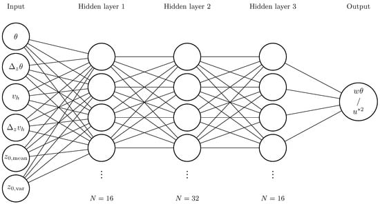
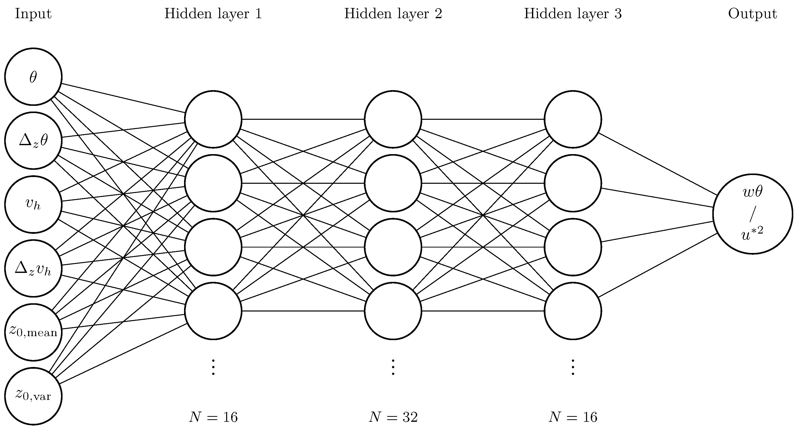
For the architecture of an MLP, several aspects have to be balanced: a larger MLP is capable of learning more complex problems [18], but it also poses a higher risk of overfitting. After several test runs, an architecture with three hidden layers that have 16, 32, and 16 neurons (Figure 1) appeared to be the best trade-off of performance and simplicity and was used as in [4]. The code was written with the python tensorflow package (version 2.16.1) [19]. The activation function is ‘relu’ for the hidden layer neurons and ‘linear’ for the output layer. The input data is normalized prior to the training process. The data samples of all simulations are shuffled and in a first step, 20% are selected for the test data set. Of the remaining data, 20% are selected for the validation set, and the rest is used for the training process. In the training process, 100 epochs are run and the batch size is 256. To rule out overfitting, the loss values of the training process and validation process are monitored. As they do not diverge during the training process, no sign of overfitting is detected. The selection of the training dataset and the initialization of the MLP influence the final result of the machine learning process. Therefore, these steps were randomized and carried out to create an ensemble of 20 members. This allows an estimation of the modeling skill and the ability to reproduce the results.
Figure 1.
Graphic scheme of the MLP. Dots indicate omitted neurons for brevity.
We measure the modeling skill of an MLP with the Pearson correlation coefficient and the normalized root mean square error (NRMSE). Due to different variances in the datasets of the two target variables, the root mean square error is normalized with the standard deviation.
Feature Importance Weighting (FIW) allows the evaluation of the relative importance of input variables [20]. This helps us to understand the calculation process of the MLP, which otherwise is a black box. Practically, the MLP runs over the dataset with the entries of one variable completely perturbed. The loss in performance compared to the unperturbed run is measured. This is performed for each of the input variables. To make it more readable, the individual loss of a variable is divided by the sum of all losses. In the following text, the MLP model we use will be referred to by the broader term ANN.
2.1.2. Polynomial Regression
With polynomial regression, the relationship of input and target variables is expressed as polynomial. The coefficients are fitted to minimize the sum of the squares of the residual. The use of polynomial regression allows the derivation of an equation and poses a simplification. It is performed using the python package scikit-learn (version 1.8.0) [21].
2.2. Large Eddy Simulations
LESs are useful tools for studying turbulence as they explicitly resolve parts of the turbulent spectrum on a limited area. The scales of the turbulent spectrum that are low pass filtered are parameterized and, therefore, computation time is saved. Depending on the process of interest and the resolution, it is valid to assume that the LES is showing a realistic behavior of the atmosphere in the three-dimensional space. LESs are therefore used as the data source for this study.
The PALM model (version 22.10) is chosen for the LESs [10]. It can be run in parallelized mode, allowing for fast computations of detailed simulations. It is used commonly for studies of the atmospheric boundary layer, urban climate, and even indoor simulations.
As noted earlier, MOST is applied at the lower boundaries of almost all models to parameterize the surface fluxes that are on subgrid scale, even in the PALM LES model. Therefore, the data at the lower boundary is the result of the MOST calculation and not of resolved turbulence modeling. Hence, it should not be used as training data because the ANN would potentially learn to reproduce the MOST parameterization. Instead, we want the ANN to reproduce explicitly calculated turbulent processes. Ref. [22] suggest that at the seventh vertical level and higher, the turbulence is sufficiently resolved. It can therefore be assumed that above this level, the relationship of fluxes, gradients, and mean variables is modeled realistically. Hence, the LES data in this layer can be regarded as robust training data. The height above ground for data usage is therefore in 40 m for mean values and in 28 m and 52 m for the difference values.
2.2.1. Simulation Scenarios
Several aspects were weighted to determine the simulation design. The horizontal domain extent should be large enough to incorporate land surface heterogeneities on a common scale. It should also be able to fit several boundary layer eddies to ensure a realistic interaction of the eddies with each other. The domain also has to be high enough to allow undisturbed boundary layer growth. To avoid the use of flow adjustment zones, cyclic boundary conditions were applied at the horizontal boundaries. A high resolution is desirable to have a more realistic representation of turbulence and to have a high density of data close to the ground. To extend the parameter space for the training data, it is useful to use multiple simulation scenarios that cover differing conditions. However, computational resources are limited. Therefore, a compromise between domain extent, resolution, and the number of simulations has to be made. The specifications of the simulations are given in Table 1.
Table 1.
Overview of LES specifications.
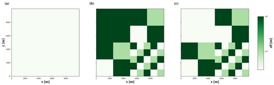
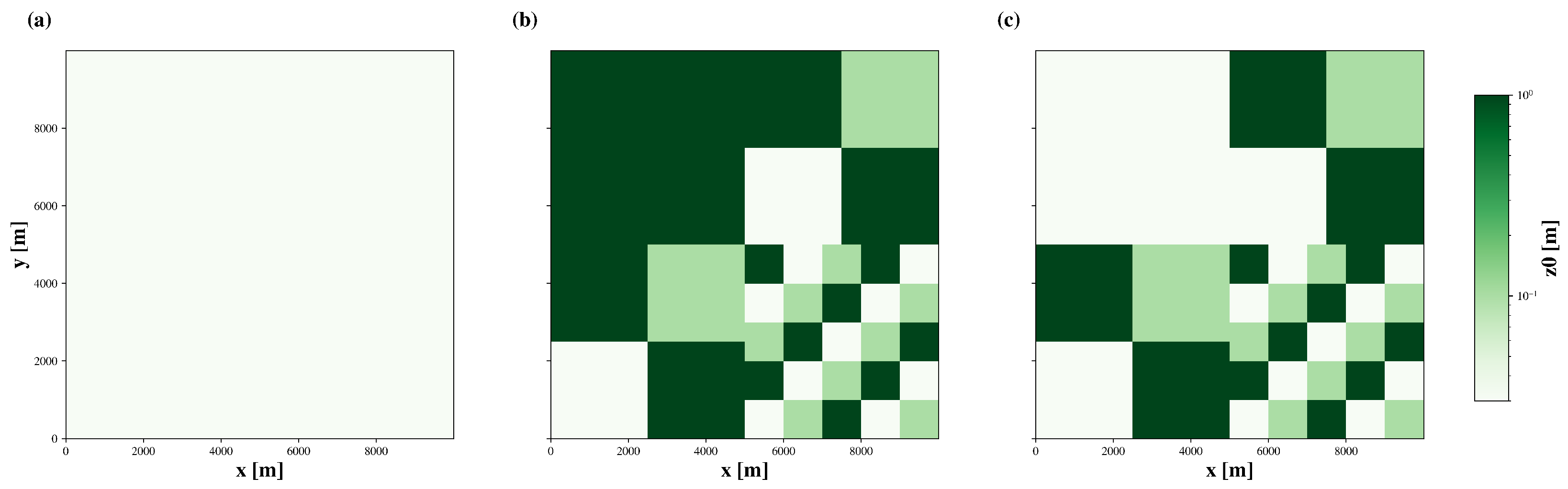
Three different domain layouts were used for the simulations: a completely homogeneous layout and two layouts that contain idealized heterogeneity patterns. For the latter two, checkerboard patterns of different sizes were invoked (Figure 2). The batches of heterogeneity have different roughness lengths. We refrain from prescribing differing values for other properties, such as albedo or soil moisture, and do not allow latent heat flux. While this poses a strong simplification, this choice has been made to avoid counteracting or superimposing effects and a dependence of the data on further parameterizations of the LES model, such as soil moisture and evapotranspiration.
Figure 2.
Surface roughness length [m] in domains A, B, and C, shown in subfigures (a), (b), and (c), respectively.
Summer and winter radiation scenarios were applied, as well as several initial wind conditions, to increase the parameter space for input and target variables. Initial wind speeds range from 0 m/s to 6 m/s. The ground temperature profile was initialized using interpolated measurement data at the Land-Atmosphere Feedback Observatory of the university of Hohenheim [23].
Each simulation covers a diurnal cycle. The simulations show the development of a convective boundary layer, including secondary circulations if surface heterogeneities are present. The diurnal cycle of radiation forces a development similar to a real boundary layer. Data is only selected for times in which the boundary layer is in a convective state. A list of all simulations can be found in Table 2.
Table 2.
Table of simulations.
2.2.2. Postprocessing
In postprocessing, a time averaging over 30 min was applied to remove turbulent fluctuations. Additionally, spatial-averaging was applied on varying box sizes to investigate the influence of spatial-averaging scales on MLP performance, similar to [14]. To reduce computing time, this procedure was not applied at all grid points but at 50 × 50 equidistant grid points. However, the reduction is deemed unproblematic as the dataset still contains 2,985,000 samples, which should be enough to train the MLP. The average of the whole domain is calculated as well, which reduces the number of samples to roughly 900 in this case. As large scale models represent grid boxes of up to several kilometers, it is of interest to examine the performance of our approach depending on the spatial-averaging scale.
3. Results
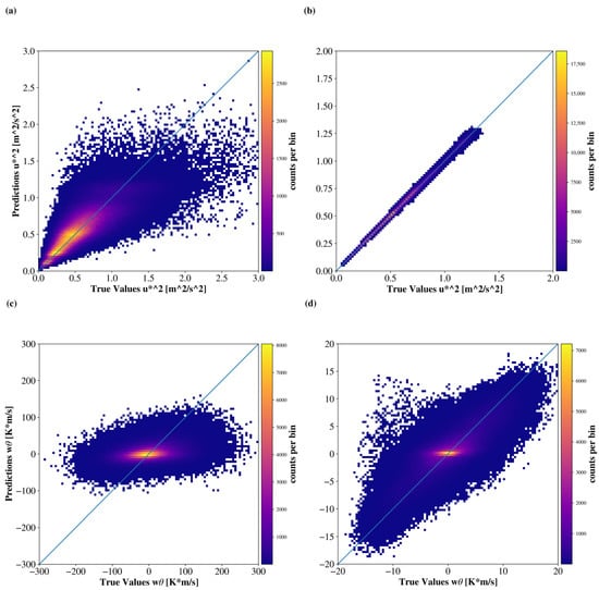
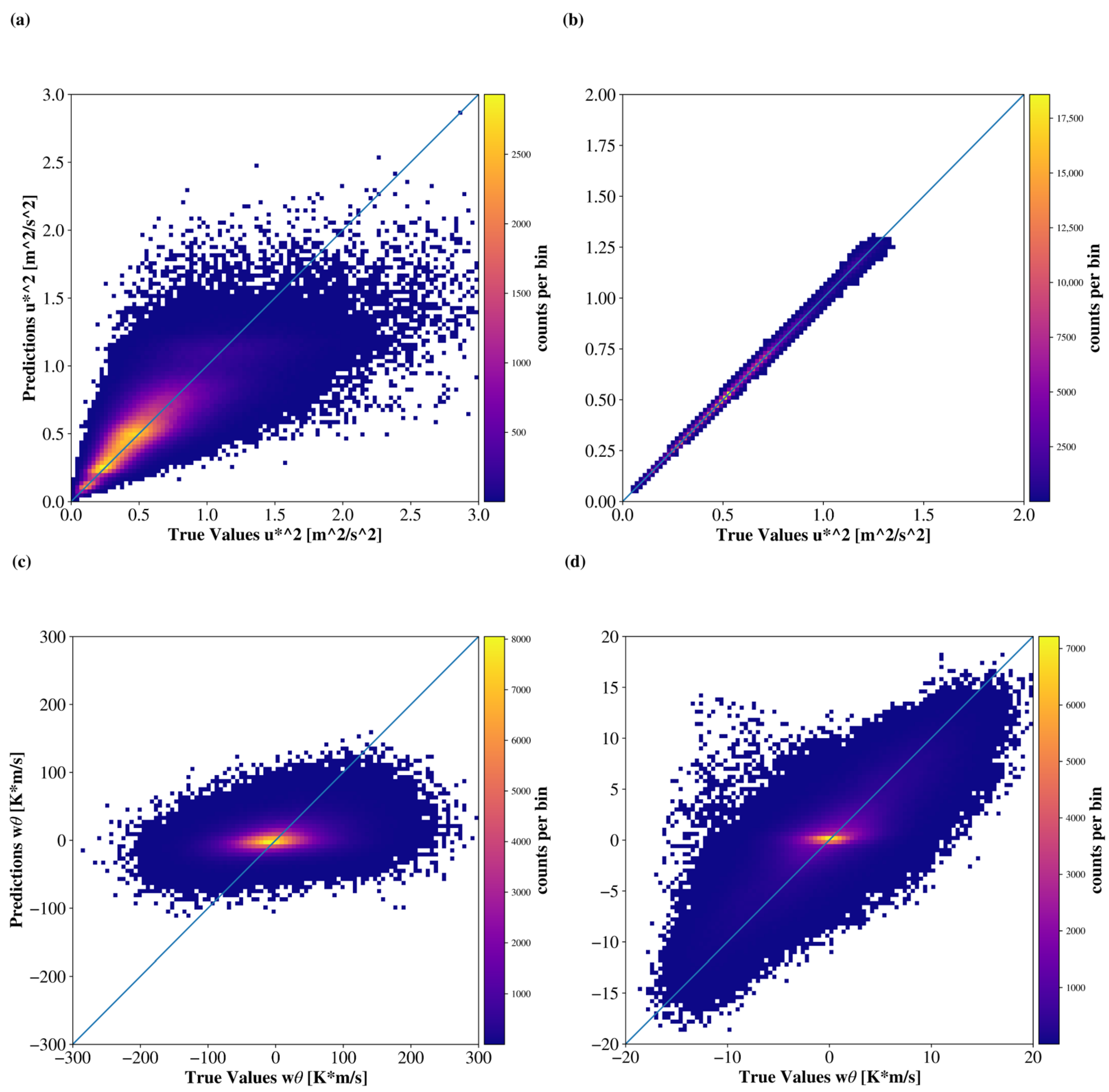
In the following, the ability of the ANN to reproduce the flux values obtained in the LES is tested. In Figure 3a,c, the ANN modeled values of MF and HF are plotted over the true values. The values were averaged over 30 min, but did not undergo any spatial averaging. In Figure 3a, a vast part of the point cloud is aligned along the diagonal, but there are also many values that exhibit a considerable uncertainty. The correlation is 0.81 and the NRMSE is 0.59. In Figure 3c, the point cloud is slightly tilted, the uncertainty is large, and in many cases the sign of the sensible heat flux is visibly calculated incorrectly. The correlation is 0.32 and the NRMSE is 0.94.
Figure 3.
Histogram of modeled versus true value of momentum flux [], (a) for single grid points and (b) spatial-averaging scale of 4000 m. The color represents the counts per bin. (c,d) shows the same plot for sensible heat flux w [K*m/s].
Given this rather poor performance particularly for HF compared to [4], we examined the data in detail. Overall, the input data are strongly variant. We believe that this is rooted in the fact that we cannot use data in immediate proximity to the ground, as described in Section 2.2.1. In the height of 40 m, surface layer eddies are well-developed and their motions modulate the relationships of the variables. For example, positive and negative values of HF occur with both positive and negative temperature differences. Although updrafts and positive values of HF would be expected to appear with an unstable temperature profile only, the inertia of surface layer eddies may cause sinking motions, even though the local temperature profile is unstable. As a result, the correlation of temperature difference and HF, which is the strongest relationship of HF with any of the input variables, is only −0.15. That makes it difficult for the ANN to find physically reasonable relationships. It therefore is not very accurate and underestimates the variance of HF. To reduce this turbulent noise, we applied spatial averaging over a box to further investigate the ability of ANNs to model the fluxes of spatially averaged data.
Figure 3b,d are the same plots as (a) and (c), but the data that is used for training and evaluation is averaged over a grid box with side length of 4000 m. Due to spatial averaging, the ANN is able to calculate the values for MF with a very high precision (R = 1.00, NRMSE = 0.05). The spread of values for HF has become much smaller. Although the point cloud is tilted along the diagonal, the uncertainty is still large. Compared to the data at single grid points, correlation is increased (0.80) and the NRMSE is decreased (0.59).
3.1. Modeling Skill
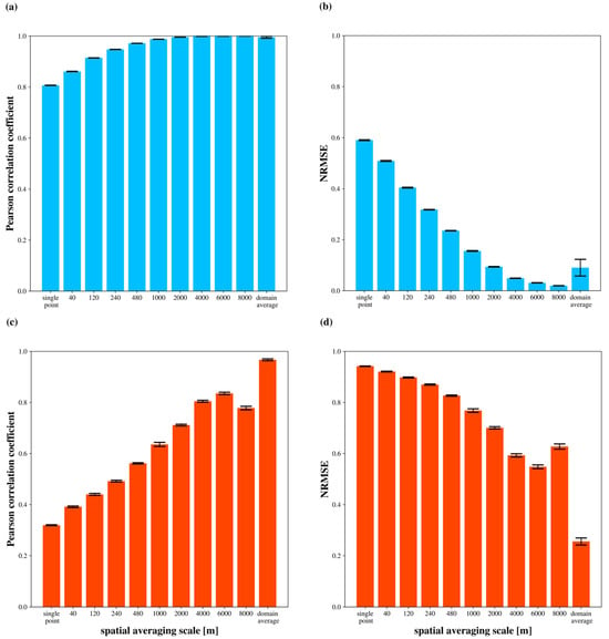
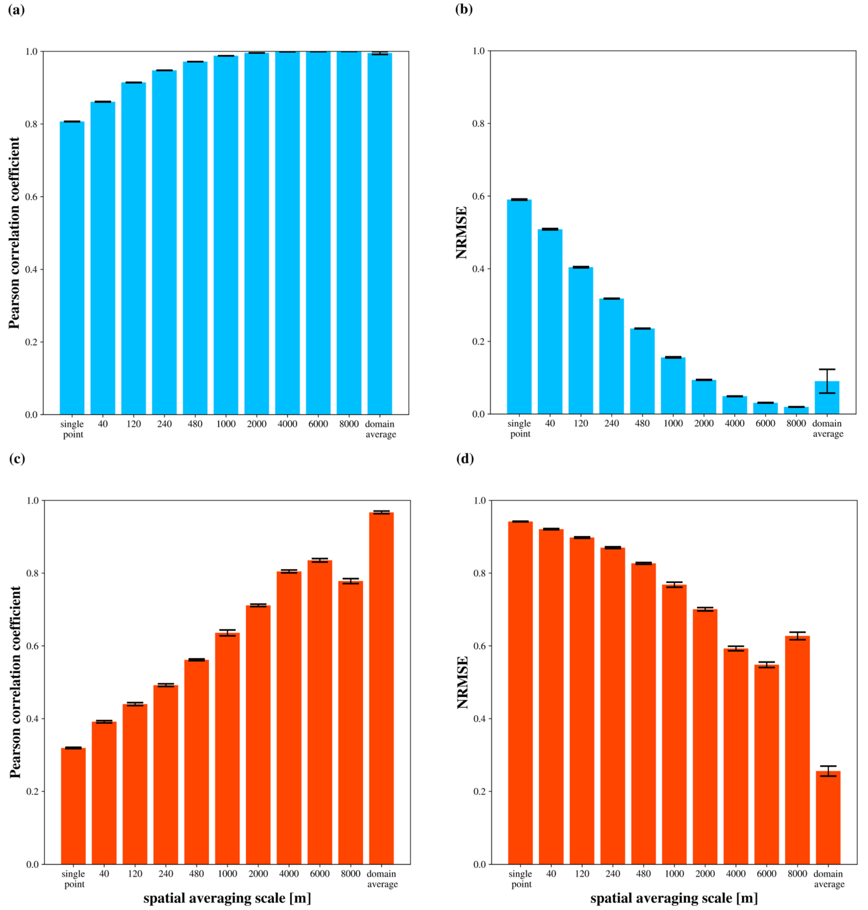
In Figure 4, the modeling skill depending on the spatial-averaging scale is shown. For every spatial-averaging scale and target variable, 20 ANNs are set up and trained. This is necessary because the initialization parameters and the selection of data batches for training alter the result of the machine learning process. It is therefore desirable to asses the statistical values of the modeling skill of an ensemble of ANNs rather than a single ANN. Table A1 holds the statistical values for the ANN ensemble for MF and Table A2 likewise for HF.
Figure 4.
Modeled versus true value Pearson correlation coefficient of momentum flux (a), NRMSE of momentum flux (b), Pearson correlation coefficient of sensible heat flux (c), and NRMSE of sensible heat flux (d), depending on the spatial averaging scale. The colored bar represents the mean value of the ensemble, and the black bar represents its standard deviation.
In Figure 4a, we see that the correlation for MF increases with increasing spatial averaging scale. Without spatial averaging, the correlation is 0.81. Above a spatial-averaging scale of 1000 m, the correlation is 0.99 or higher. In Figure 4b, the NRMSE of MF is around 0.59 when no spatial averaging is applied and decreases to 0.02 for the 8000 m spatial-averaging scale. For the domain average, the NRMSE increases to about 0.09. For the domain average, correlation decreases and NRMSE increases. This is likely a result of the decreased number of samples for the domain average, as there is only one value per timestep compared to 2500 for the other spatial-averaging scales. In Figure 4c, there is also a positive trend in correlation with increased spatial averaging for HF. However, there is a local minimum for the 8000 m averaging scale. Only the domain-averaged data has a correlation of close to 1. In Figure 4d, for HF, without spatial averaging, the NRMSE is around 0.94 and drops to 0.55 for 6000 m. In analogy to the correlation, there is a local maximum at 8000 m. For the domain average, the NRMSE is 0.26.
In the case of the domain average, the circulation pattern in the simulation, which is averaged over, contains the total HF from the surface to the atmosphere. We suspect that the ANN therefore only has to learn some kind of conservation of energy. In the other cases, it additionally has to assume to what extent updrafts or downdrafts are present in the averaging window. This seems to be more difficult and could be the reason for the lower correlation. In general, this seems to be easier for a larger spatial-averaging scale. When rerunning the analysis with data from a smaller test domain, there is a similar increase in the modeling skill when using the domain average (not shown). We can therefore rule out that this increase in the modeling skill is particularly connected to the averaging of turbulence over 10,000 m. Instead, it appears to be a result of the complete domain being included in the spatial-averaging process.
For the decrease in performance at the 8000 m spatial-averaging scale (Figure 4c,d), we hypothesize that this is because the box size approaches the size of the whole domain. Given that the domain average of HF is almost 0 K m/s (not shown), the value of an averaging window could be expressed as the negative value of the area outside the averaging window. When the spatial-averaging scale approximates the domain size, the area outside of the averaging window becomes smaller, so that the turbulent structures of the surface layer are not averaged out because they are of similar size. Instead, there is a larger uncertainty due to turbulent noise. The minimum in skill at the 8000 m spatial-averaging scale could therefore be an artifact of this combination of spatial-averaging scale and domain size.
The flux calculation with MOST according to [24] was tested on our data as well. The results can be found in Table A3 and Table A4. For MF, the correlation is in all cases less than that of the ANN and below 0.8. For HF, only for the domain-averaged data the correlation is notable (0.76), in all other cases the correlation is below 0.1. We assume that low values of and , as well as the turbulent noise, are the cause for the lack of skill.
In general, the ANN models MF better than HF. The better predictability of MF is favored by higher correlations with individual input variables (not shown).
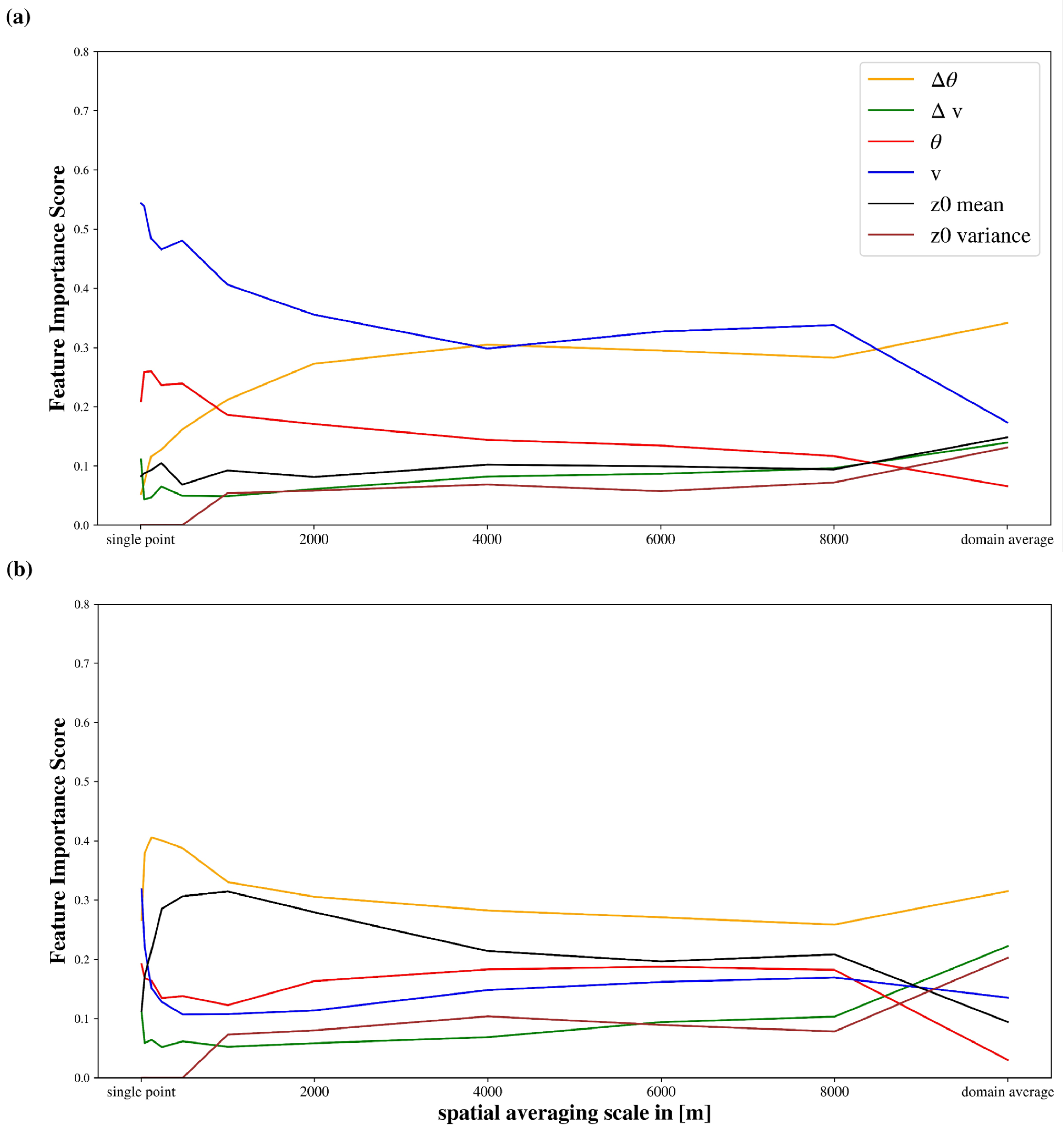
3.2. Feature Importance Weighting
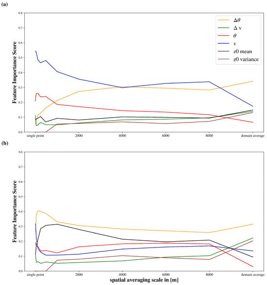
Figure 5 shows the ensemble mean Feature Importance Score (FIS) of the input variables. The numerical values can be found in Table A5 and Table A6. For MF (Figure 5a), at small spatial-averaging scales, horizontal wind speed is the most important variable, followed by potential temperature . The FIS of the vertical wind speed difference , the vertical potential temperature difference , and mean are of similar magnitude, while variance is 0 (because there is no variance at a single grid point). With increasing spatial-averaging scale, the FIS of decreases, while it increases for . The FIS of variance is 0 until a spatial-averaging scale of 1000 m, for larger spatial-averaging scales it is close to the values of and mean. The FIS of the latter two stays relatively constant with increasing spatial-averaging scale. For the domain average, the relative importance of input variables changes considerably. has the highest FIS, followed by , mean, , and variance, which are of very similar magnitude, and then .
Figure 5.
Ensemble mean Feature Importance Score of input variables depending on the spatial-averaging scale (a) for the calculation of momentum flux and (b) for the calculation of sensible heat flux.
For HF in Figure 5b, at a single grid point and have the highest FIS. , , and mean are less important. In general, the FIS is strongly variant at spatial-averaging scales smaller than 1000 m. At larger spatial-averaging scales, has the highest FIS, followed by mean, , and . and variance have the lowest FIS. For the domain average, there are clear differences to the smaller spatial-averaging scales. Notably, the difference variables are the most important variables for the domain average of HF. has the highest FIS, followed by and variance. , mean and have the lowest FIS.
The domain average of HF is the only case where variance has a higher FIS than mean. variance is an expression of the heterogeneity of the surface, which could have an impact on how well convection is organized. This could be particularly important for the domain average. For cases with smaller spatial-averaging scales, the location of surfaces and their favorability for updrafts, that is mean, seem to be more important. However, it must also be noted that tests have shown that the exclusion of variance had only marginal effects on the performance of the ANN.
For both target variables, the relative importance of input variables varies greatly on the sub-kilometer spatial-averaging scale and from 8000 m to the domain average. In the case of the sub-kilometer spatial-averaging scale, it should be noted that the modeling skill, at least for HF, is quite low (Figure 4). Therefore, the significance of the FIW is reduced in these spatial-averaging scales. On the other end of the spatial-averaging scale spectrum, there are strong differences in FIS when we change to the domain average. That means we change from an open averaging window to a closed one. Mesoscale models also have to assume a closed average window for a grid cell, which makes this case especially relevant.
3.3. Reduction of Input Variables and Polynomial Regression
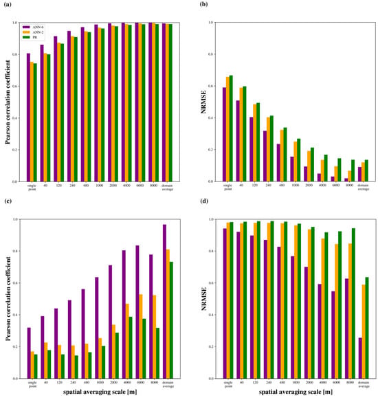
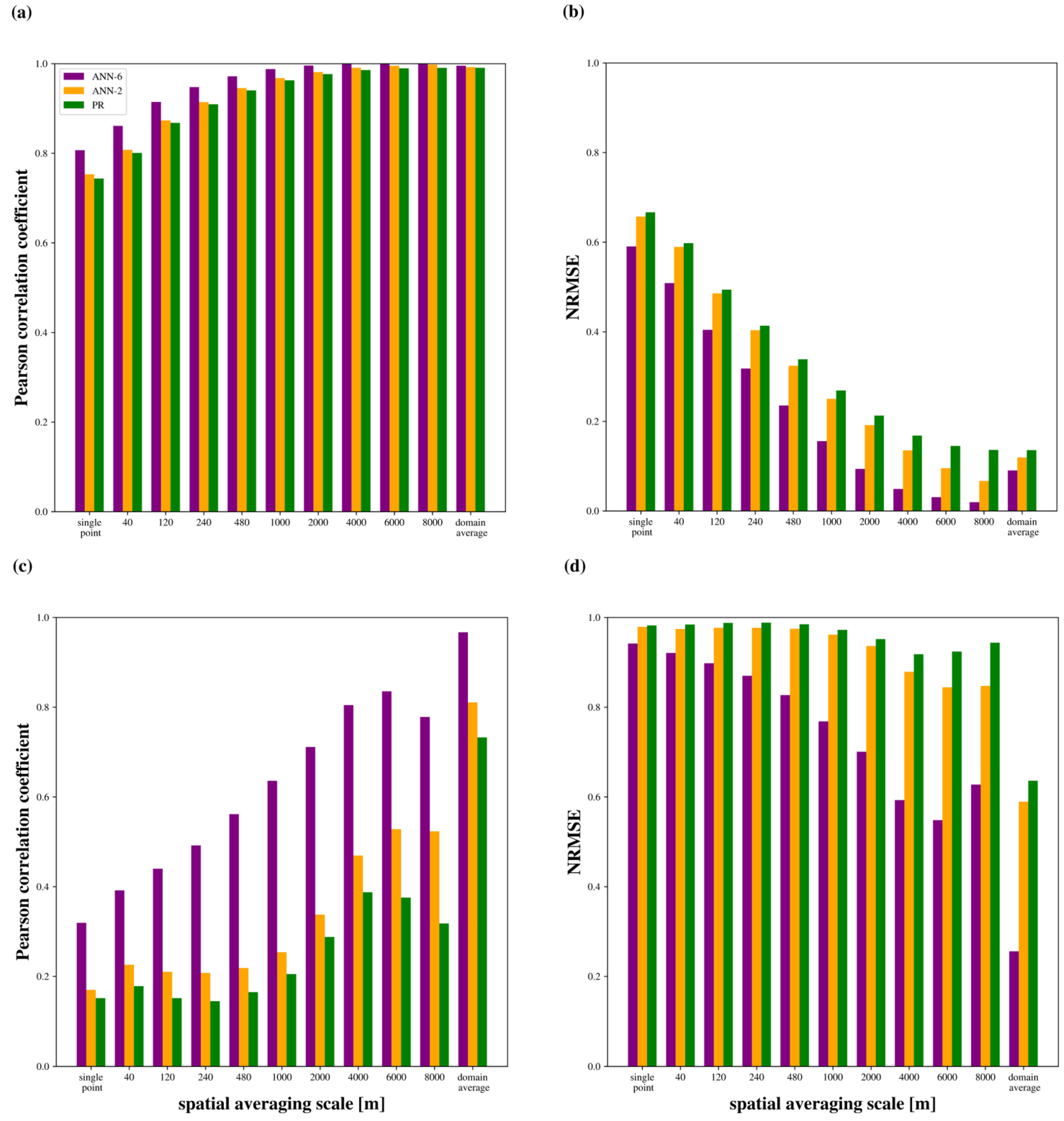
In this subsection, the possibility of further simplification of the calculation process is explored. An ANN (ANN-2) and a second-degree polynomial regression model (PR), both with two input variables, are compared to the ANN with six input variables (in this subsection referred to as ANN-6). The two input variables are selected based on the FIS for the respective target variable at the spatial-averaging scale of 1000 m. That is, for MF, and and for HF, and mean.
Figure 6a shows the correlation for the calculation of MF. Table A7 and Table A8 hold the corresponding numbers. For every spatial-averaging scale, ANN-6 has the highest correlation and PR the lowest. Also, ANN-2 has a higher correlation than PR at every spatial-averaging scale, but the difference is less than 0.01. The difference of PR and ANN-6 is 0.06 for single grid point values and decreasing for larger spatial-averaging scales.
Figure 6.
Modeled versus true value Pearson correlation coefficient of momentum flux (a), NRMSE of momentum flux (b), Pearson correlation coefficient of sensible heat flux (c), and NRMSE of sensible heat flux (d), depending on the spatial averaging scale. The colored bar represents the mean value for either ANN-6, ANN-2, or PR. All values represent the ensemble mean.
Figure 6b shows the NRMSE for the calculation of MF. ANN-6 has the lowest NRMSE and PR has the highest NRMSE. At smaller spatial-averaging scales, the difference in NRMSE between PR and ANN-6 is 0.06 (single grid point) and increases towards larger spatial-averaging scales (0.11 at 6000 m). The difference of PR and ANN-2 is small at single grid points (0.01) and has its maximum at 8000 m (0.07). In contrast to ANN-6 and ANN-2, PR hast its lowest NRMSE at the domain average, resulting in a smaller difference to the other approaches in this case. The reason for this should be that the reduced number of data samples does not affect the polynomial regression method in the same way it does with the ANNs.
In Figure 6c, the correlation for the calculation of HF is shown. The correlation of PR is below 0.4 for every spatial-averaging scale except the domain average (0.73). The correlation for ANN-2 is in every case higher than that for PR, but below 0.6 for every spatial-averaging scale but the domain average (0.81). ANN-6 has a much higher correlation than the other approaches at all spatial-averaging scales. Interestingly, both PR and ANN-2 have several local minima in correlation depending on the spatial-averaging scale. The difference between PR and ANN-2 is rather small (0.02) for smaller spatial-averaging scales, but growing towards larger spatial-averaging scales (0.20 at 8000 m). For the domain average, however, this difference is again smaller.
In Figure 6d, the NRMSE for the calculation of HF is shown. At all spatial scales, the NRMSE is highest for PR and lowest for ANN-6. For PR and ANN-2, the NRMSE has several local maxima, and the difference between the two approaches is greater for larger spatial-averaging scales, with ANN-2 having a smaller NRMSE in all cases. Only for the domain average, NRMSE has a strong decrease for all three approaches. However, for ANN-6, it is less than half than that of PR and ANN-2.
Overall, the performance of PR and ANN-2 is worse than that of ANN-6. It can be stated that the reduction to two input variables comes with a strong decrease in performance, especially for the calculation of HF.
Also, ANN-2 outperforms PR in all cases. For our dataset, ANNs seem to be more suited to reproduce MF and HF than polynomial regression, which could be an indicator that ANNs are better suited to model the relationships of input and target variables in the context of turbulent flux calculation.
4. Discussion
The first goal of this study is to examine the potential of the ANN to reproduce the MF and HF that was simulated in an LES. The analysis is carried out at a range of spatial-averaging scales, from single grid points to the whole domain. Modelling the fluxes at single points is the simplest setup to test the ANN. It is the simulation analogy to eddy covariance station data and is therefore suited to compare with studies that use such observation data [25,26,27]. Since the simulation data is available on a three-dimensional field, it is also of interest how the ANN performance changes if the spatial-averaging scale is increased and more turbulent noise is filtered out. The domain average case is particularly interesting because it averages over all turbulent structures that are present in the simulation. Figure 4 shows that for MF, the ANN can model the value quite well, and for HF it works only on larger spatial-averaging scales. The domain-averaged values are particularly well-modeled by the ANN. Increasing the modeling skill for larger spatial averaging is expected because turbulence is filtered out. The result is similar to [14], where the MOST calculation of MF improves in accuracy with spatial averaging.
When reducing the number of input variables to two and applying an ANN or polynomial regression, there are slight decreases in performance for MF and more pronounced decreases for HF. For HF, the increase in performance towards larger spatial-averaging scales is not monotonic and the difference to the ANN with six input variables is quite large. Therefore, a calculation with two input variables seems to be too simplistic in most cases, especially for the calculation of HF. It should also be noted that the ANN performs better than polynomial regression in every case, although the order of magnitude of this difference varies case by case. Our interpretation is that ANNs have a larger capability to find interrelations in our data than polynomial regression.
Other studies that use machine learning to calculate MF and HF mostly use eddy covariance station data to do so [4,11,12]. In [4,11,12], ANNs tested and trained on eddy covariance measurement data reach much higher correlations than our ANN does for data at single grid points. This could be due to the increased height above ground of our data. It enables a stronger influence of turbulent structures. Furthermore, the very pronounced heterogeneities of the land surface in our data could have a negative effect on predictability. In addition, some of these studies used different input variables. Technically, this means that on this spatial scale, the input variables provided to our ANN give only limited information on the driving factors of the flux values.
When comparing the calculation, the ANN is reaching much higher correlations and lower uncertainties than the MOST calculation (Table A3 and Table A4). The better performance of ML approaches coincides with [4,12]. In [11], MOST and the ANN have a similar predictive skill and depending on the case, one or the other technique performs better. However, they use simpler ANN architectures. In our study, the MOST calculation has poor results. It must be stated, however, that the MOST calculation was developed with observation data collected at lower heights than that in the data available in this study [24]. This is a contrast and disadvantage to our ANN model, which was trained on this kind of data. Even though this result is a positive signal regarding the potential of this method, we think the comparability to MOST on these data is compromised.
In summary, the ANN is capable of deriving MF and HF, but especially for HF, we find constraints to the modeling skill in our set-up that lead to partially non-satisfying results.
The second objective of this study was to identify problems that would have to be overcome to develop a flux parameterization with an ANN based on LES training data. The possibility to use spatially averaged data poses the question of which spatial scale is most relevant to develop a parameterization. On the one hand, data at single grid points allows a verification on eddy covariance station data and the comparison with common approaches on these data. On the other hand, in a mesoscale model, the parameterization of the surface fluxes represents the average of a whole grid cell, which can translate to several square kilometers of surface area. Using a bigger spatial-averaging scale is therefore closer to what a mesoscale model needs to simulate. Also, there is no horizontal advection in a mesoscale model between the lowest vertical level and the ground, so the domain average case is similar to this application. The changes in FIS for different spatial-averaging scales underline that it might even be necessary to specify parameterizations depending on which spatial scale and which case is to be represented.
It would be desirable to be able to use data from lower levels, regardless of whether one is interested in domain-averaged values or single grid point values. This would require a higher resolution of the LES. Given that there are computational limitations, a higher resolution would require a smaller domain, which decreases the ability to simulate the boundary layer circulation and investigate its interaction with land surface heterogeneities. In a future study, one could therefore test this approach with a smaller domain. Also, GPU computing could accelerate computations and enable higher resolutions.
In this study, stable conditions are excluded, because LES models do not reproduce stable conditions realistically [28]. A parameterization however would also need to work in stable conditions. The inclusion of stable conditions in the current approach therefore is dependent on improvements in LES modeling. The current ensemble of simulations is an attempt to cover a range of unstable conditions over different domains and to test and train the ANN on it. Therefore, it is an assessment of the potential of this method. The development of a parameterization however requires generalizability. ANNs do not extrapolate well beyond the parameter space in which they were trained [29]; hence, there is a need to identify and cover this parameter space of real-world conditions. That means that the realistic range of input and target variables would have to be determined from observation data so that all realistic combinations of values are included in the training data.
The perhaps most important issue in our approach is the neglect of latent heat fluxes. Since latent heat flux and sensible heat flux are strongly interacting [1], a new parameterization would require an inclusion of latent processes in the training data and as input variables or the ANN. It was left out because in the LES the (evapo)transpiration would be parameterized, leading to the ANN potentially reproducing these parameterizations that have a high degree of uncertainty themselves. However, in a next step, one could include latent heat processes in the LES data and training process and verify the results afterwards by comparing the ANN model to observation data. This would, however, require a good spatial and temporal coverage in the observation data to be able to apply the ANN model.
An advantage of LES is its spatial data availability. Hence, the performance of a flux parameterization can be mapped and analyzed. This might help to understand location-related strengths or shortcomings of the approach. To demonstrate this potential, Figure A1 shows the correlation of the data at every point in the Bs1d scenario. We see that the ANN is reaching a high correlation in a relatively homogeneous area in the center, left, top, and bottom (they are adjacent to each other due to cyclic boundary conditions).
In this study, we come to the conclusion that this method shows potential in calculating fluxes, but several changes would be necessary to develop a parameterization. These issues could be solved by technological developments, further testing to determine the most applicable approach, and a framework to assure generalizability.
The third objective was to assess the role of surface heterogeneity. In our study, the input variable to express surface heterogeneity is the spatial variance of the roughness length. This is a common and simple approach [30] and has the benefit that it applies to the entire area and that no positional information is required. In a more sophisticated way, one could try to establish a positional relationship of heterogeneity elements to the measurement location; for example, as introduced in [31], or even account for the wind direction and focus on upstream heterogeneity elements. But the application of this approach would not be straightforward, because heterogeneity elements could be present on a spectrum of scales. Moreover, continuous changes in wind direction and speed could undermine the possibility to relate the state of turbulence to the upstream surface. However, we want to focus on methods that would be applicable while running a mesoscale model, and the implemented method has a very low computational demand and is simple to apply to various spatial-averaging scales. In the real world, heterogeneities are present in other physical properties, such as albedo, soil moisture, and vegetation cover. If the spatial distributions of different heterogeneities in relation to each other are to be accounted for, it will significantly complicate the calculation of one or more surface heterogeneity parameters. Therefore, in a follow-up study, one could include all heterogeneity types in the LES setup and test a heterogeneity variable that is based on discrete land surface types.
We try to quantify the importance of surface heterogeneity with the FIS of variance (Figure 5). While for small spatial-averaging scales the FIS of variance is low, it is increasing for higher spatial-averaging scales. The strongest influence is registered for the domain average. For the domain average, the FIS is relatively high and the modeling skill is high as well. In fact, tests show that leaving out single input variables in this case reduces the modeling skill only marginally. Therefore, while the FIS of variance is high, the ANN would reach a similar modeling skill without variance.
Ref. [13] measure the relative importance of input variables when modeling domain-averaged sensible dispersive heat fluxes with a machine learning technique. They rate the importance of a heterogeneity parameter higher than that of . However, the importance of heterogeneity might be higher for the dispersive flux than for the total flux. In addition, they include a stability parameter, which is not used in our study, that might contain information that our ANN partially extracts from , and thereby decrease the FIS of . Therefore, the different order in importance ratings is not necessarily a contradiction.
5. Conclusions
A set of 12 LESs, containing idealized heterogeneity features, was run under convective conditions with varying wind and irradiation scenarios and used as the ‘observation system experiment’. The data was averaged over 30 min and different spatial scales from single-grid point to the domain average. An ANN architecture (16-32-16) was tested on its potential to reproduce the fluxes of momentum and sensible heat with six input variables provided.
The first research question was how well the ANN can model MF and HF calculated by an LES. The modeling skill was higher for MF than for HF. In general, the modeling skill was higher for larger spatial-averaging scales. The correlation improved from 0.81 (single-grid point) to 1.00 (4000 m) for MF and from 0.32 (single-grid point) to 0.80 (4000 m) for HF. The domain average was particularly well-modeled for both target variables. A Feature Importance Weighting was carried out to quantify the influence of input variables. In particular, for the domain average, the relative importance of input variables changes heavily. The reduction to two input variables for both an ANN and polynomial regression comes with a substantial loss in performance.
The second objective was to investigate possible problems of this approach for the development of a flux parameterization for mesoscale models. Several possible constraints are identified: Latent processes and stable conditions need to be included, a higher resolution in the LES (and hence a lower height of analysis) would be desirable, and a framework is needed to determine the required variety in input and output variables. Moreover, the optimal spatial-averaging scale for this task remain to be determined.
The third research question was to examine the benefit of using surface heterogeneity information for modeling. The surface heterogeneity was represented in variance. In most cases, it appears to be a less influential variable, although its importance is increasing with spatial-averaging scale. Other (more extensive) surface heterogeneity parameters (for example, [31]) will be tested for their relative importance and applicability in an upcoming study.
Author Contributions
Conceptualization, B.K. and M.B.; methodology: B.K. and M.B.; software, B.K.; validation, B.K.; formal analysis, B.K., M.B., and V.W.; investigation, B.K.; resources, M.B.; data curation, B.K.; writing—original draft preparation, B.K.; writing—review and editing, M.B. and V.W.; visualization, B.K.; supervision, M.B.; project administration, M.B.; funding acquisition, M.B. All authors have read and agreed to the published version of the manuscript.
Funding
This research was funded by Deutsche Forschungsgemeinschaft (DFG) Award Nr. 456675194.
Institutional Review Board Statement
Not applicable.
Informed Consent Statement
Not applicable.
Data Availability Statement
The simulation data and all codes are available upon personal request to the corresponding author.
Acknowledgments
Matthias Karlbauer (ECMWF) supported the work process related to machine learning. The script for the MOST calculation was provided by Juan Manuel Valencia. User support for LES calculations was provided by the PALM Developers Team. The computational resources were provided by the Höchstleistungrechenzentrum Stuttgart (HLRS). During the preparation of this study, the authors used the AI assistant ChatGPT (OpenAI, GPT-4, accessed via API from 2024 to 2026) for support with code development and debugging. The authors have reviewed and edited all AI-generated output and take full responsibility for the content of this publication.
Conflicts of Interest
The authors declare no conflicts of interest.
Abbreviations
The following abbreviations are used in this manuscript:
| ANN | Artificial Neural Network |
| LES | Large Eddy Simulation |
| MOST | Monin Obukhov Similarity Theory |
| RMSE | Root Mean Square Error |
| MF | Momentum Flux |
| HF | Sensible Heat Flux |
| FIW | Feature Importance Weighting |
| FIS | Feature Importance Score |
| MLP | Multilayer Perceptron |
| NRMSE | Normalized Root Mean Square Error |
| ANN-6 | ANN with six input variables |
| ANN-2 | ANN with two input variables |
| PR | Polynomial Regression Model with two input variables |
Appendix A
Table A1.
Pearson correlation coefficient and NRMSE of calculation of momentum flux (ensemble values) depending on the spatial-averaging scale.
Table A2.
Pearson correlation coefficient and NRMSE of calculation of sensible heat flux (ensemble values) depending on the spatial-averaging scale.
Table A3.
Pearson correlation coefficient and NRMSE for MOST calculation of momentum flux depending on the spatial-averaging scale.
Table A4.
Pearson correlation coefficient and NRMSE for MOST calculation of sensible heat flux depending on the spatial-averaging scale.
Table A5.
Feature importance score of input variables (ensemble values) for momentum flux, depending on the spatial-averaging scale.
Table A6.
Feature importance score of input variables (ensemble values) for sensible heat flux, depending on the spatial-averaging scale.
Table A7.
Pearson correlation coefficient and NRMSE of calculation of momentum flux of ANN-6, ANN-2, and PR. All numbers are ensemble mean values.
Figure A1.
Map of Pearson correlation coefficient of modeled and true value of sensible heat flux, spatial-averaging scale 4000 m, scenario Bs1d, use of a single ensemble member.
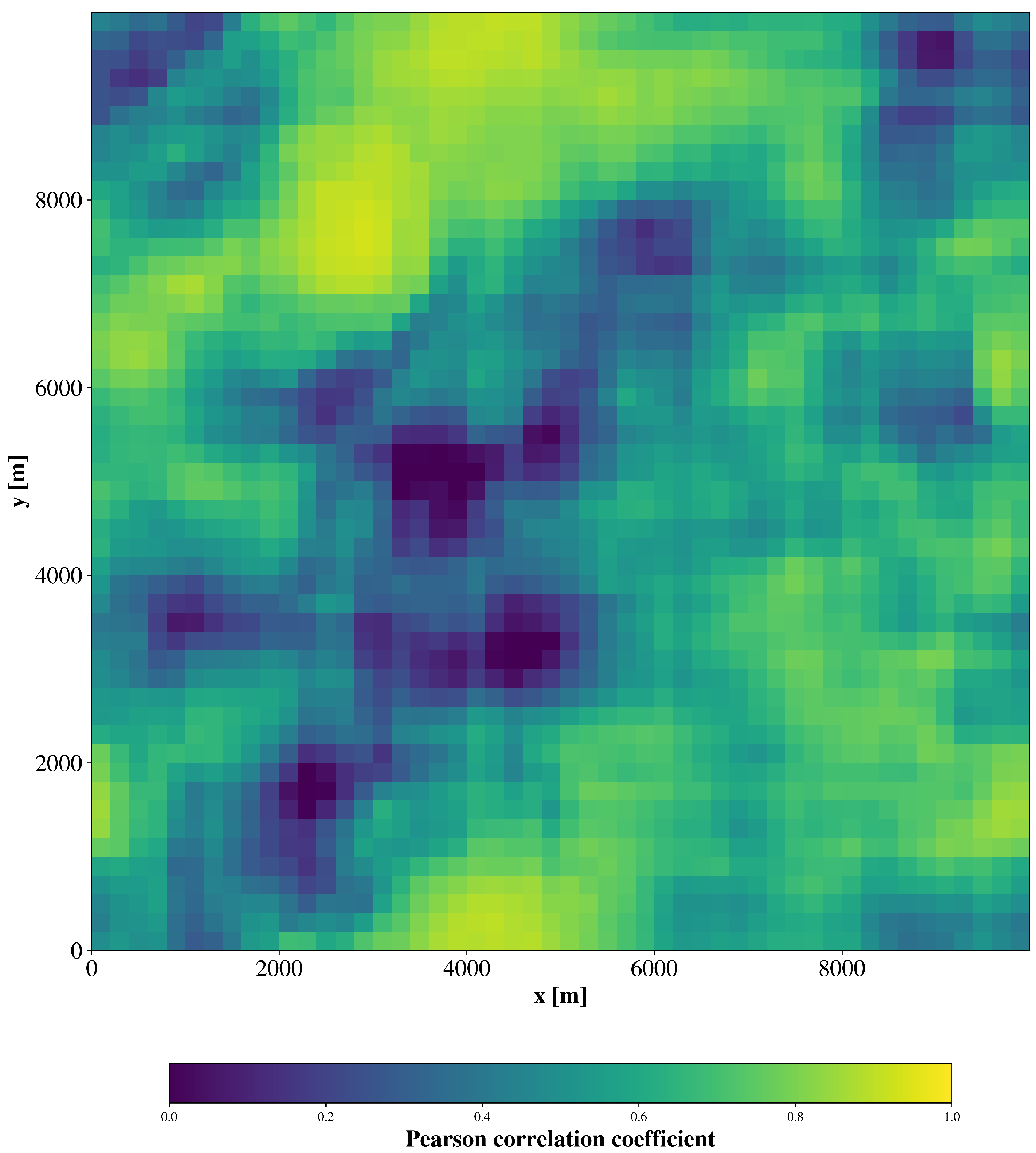
Table A8.
Pearson correlation coefficient and NRMSE of calculation of sensible heat flux of ANN-6, ANN-2, and PR, all numbers are ensemble mean values.
References
- Stull, R. An Introduction to Boundary Layer Meteorology; Springer: Berlin/Heidelberg, Germany, 1988. [Google Scholar] [CrossRef] [Scilit]
- Monin, A.; Obukhov, A. Basic laws of turbulent mixing in the surface layer of the atmosphere. Contrib. Geophys. Inst. Acad. Sci. 1954, 151, e187. [Google Scholar]
- Högström, U. Review of Some Basic Characteristics of the Atmospheric Surface Layer. In Boundary-Layer Meteorology 25th Anniversary Volume, 1970–1995: Invited Reviews and Selected Contributions to Recognise Ted Munn’s Contribution as Editor over the Past 25 Years; Garratt, J.R., Taylor, P.A., Eds.; Springer: Dordrecht, The Netherlands, 1996; pp. 215–246. [Google Scholar] [CrossRef] [Scilit] [PubMed]
- Wulfmeyer, V.; Valencia Pineda, J.; Otte, S.; Karlbauer, M.; Butz, M.; Lee, T.; Rajtschan, V. Estimation of the Surface Fluxes for Heat and Momentum in Unstable Conditions with Machine Learning and Similarity Approaches for the LAFE Data Set. Bound.-Layer Meteorol. 2023, 186, 337–371. [Google Scholar]
- Bou-Zeid, E.; Anderson, W.; Katul, G.; Mahrt, L. The Persistent Challenge of Surface Heterogeneity in Boundary-Layer Meteorology: A Review. Bound.-Layer Meteorol. 2020, 177, 227–245. [Google Scholar] [CrossRef] [Scilit]
- Margairaz, F.; Pardyjak, E.; Calaf, M. Surface Thermal Heterogeneities and the Atmospheric Boundary Layer: The Thermal Heterogeneity Parameter. Bound.-Layer Meteorol. 2020, 177, 49–68. [Google Scholar] [CrossRef] [Scilit]
- Simon, J.; Bragg, A.; Dirmeyer, P.; Chaney, N. Semi-Coupling of a Field-Scale Resolving Land-Surface Model and WRF-LES to Investigate the Influence of Land-Surface Heterogeneity on Cloud Development. J. Adv. Model. Earth Syst. 2021, 13, e2021MS002602. [Google Scholar] [CrossRef] [Scilit]
- Tian, J.; Zhang, Y.; Klein, S.; Öktem, R.; Wang, L. How Does Land Cover and Its Heterogeneity Length Scales Affect the Formation of Summertime Shallow Cumulus Clouds in Observations From the US Southern Great Plains? Geophys. Res. Lett. 2022, 49, e2021GL097070. [Google Scholar] [CrossRef] [Scilit]
- Poll, S.; Shrestha, P.; Simmer, C. Grid resolution dependency of land surface heterogeneity effects on boundary-layer structure. Q. J. R. Meteorol. Soc. 2022, 148, 141–158. [Google Scholar] [CrossRef] [Scilit]
- Maronga, B.; Banzhaf, S.; Burmeister, C.; Esch, T.; Forkel, R.; Fröhlich, D.; Fuka, V.; Gehrke, K.F.; Geletič, J.; Giersch, S.; et al. Overview of the PALM model system 6.0. Geosci. Model Dev. 2020, 13, 1335–1372. [Google Scholar] [CrossRef] [Scilit]
- Leufen, L.H.; Schädler, G. Calculating the turbulent fluxes in the atmospheric surface layer with neural networks. Geosci. Model Dev. 2019, 12, 2033–2047. [Google Scholar] [CrossRef] [Scilit]
- Muñoz-Esparza, D.; Becker, C.; Sauer, J.; Gagne, D., II; Schreck, J.; Kosović, B. On the Application of an Observations-Based Machine Learning Parameterization of Surface Layer Fluxes Within an Atmospheric Large-Eddy Simulation Model. J. Geophys. Res. Atmos. 2022, 127, e2021JD036214. [Google Scholar] [CrossRef] [Scilit]
- Wanner, L.; Jung, M.; Paleri, S.; Butterworth, B.; Desai, A.; Sühring, M.; Mauder, M. Towards Energy-Balance Closure with a Model of Dispersive Heat Fluxes. Bound.-Layer Meteorol. 2024, 190, 25. [Google Scholar] [CrossRef] [Scilit]
- Liu, S.; Zeng, X.; Dai, Y.; Yuan, H.; Wei, N.; Wei, Z.; Lu, X.; Zhang, S.; Li, X. Scale-Dependent Estimability of Turbulent Flux in the Unstable Surface Layer for Land Surface Modeling. J. Adv. Model. Earth Syst. 2023, 15, e2022MS003567. [Google Scholar] [CrossRef] [Scilit]
- Bodini, N.; Lundquist, J.K.; Optis, M. Can machine learning improve the model representation of turbulent kinetic energy dissipation rate in the boundary layer for complex terrain? Geosci. Model Dev. 2020, 13, 4271–4285. [Google Scholar] [CrossRef] [Scilit]
- Schmidhuber, J. Deep learning in neural networks: An overview. Neural Netw. 2015, 61, 85–117. [Google Scholar] [CrossRef] [Scilit] [PubMed]
- Goodfellow, I.; Bengio, Y.; Courville, A. Deep Learning; MIT Press: Cambridge, MA, USA, 2016; Available online: http://www.deeplearningbook.org (accessed on 26 March 2026).
- Zhang, C.; Bengio, S.; Hardt, M.; Recht, B.; Vinyals, O. Understanding deep learning requires rethinking generalization. arXiv 2016, arXiv:1611.03530. [Google Scholar]
- Abadi, M.; Agarwal, A.; Barham, P.; Brevdo, E.; Chen, Z.; Citro, C.; Corrado, G.; Davis, A.; Dean, J.; Devin, M.; et al. TensorFlow: Large-Scale Machine Learning on Heterogeneous Systems; Tensorflow: Mountain View, CA, USA, 2015. [Google Scholar]
- Breimann, L. Random Forests. Mach. Learn. 2001, 45, 5–32. [Google Scholar] [CrossRef] [Scilit]
- Pedregosa, F.; Varoquaux, G.; Gramfort, A.; Michel, V.; Thirion, B.; Grisel, O.; Blondel, M.; Prettenhofer, P.; Weiss, R.; Dubourg, V.; et al. Scikit-learn: Machine Learning in Python. J. Mach. Learn. Res. 2011, 12, 2825–2830. [Google Scholar]
- Maronga, B.; Knigge, C.; Raasch, S. An Improved Surface Boundary Condition for Large-Eddy Simulations Based on Monin–Obukhov Similarity Theory: Evaluation and Consequences for Grid Convergence in Neutral and Stable Conditions. Bound.-Layer Meteorol. 2020, 174, 297–325. [Google Scholar] [CrossRef] [Scilit]
- Späth, F.; Rajtschan, V.; Weber, T.K.D.; Morandage, S.; Lange, D.; Abbas, S.S.; Behrendt, A.; Ingwersen, J.; Streck, T.; Wulfmeyer, V. The land–atmosphere feedback observatory: A new observational approach for characterizing land–atmosphere feedback. Geosci. Instrum. Methods Data Syst. 2023, 12, 25–44. [Google Scholar] [CrossRef] [Scilit]
- Dyer, A.J.; Hicks, B.B. Flux-gradient relationships in the constant flux layer. Q. J. R. Meteorol. Soc. 1970, 96, 715–721. [Google Scholar] [CrossRef] [Scilit]
- Baldocchi, D.; Falge, E.; Gu, L.; Olson, R.; Hollinger, D.; Running, S.; Anthoni, P.; Bernhofer, C.; Davis, K.; Evans, R.; et al. FLUXNET: A New Tool to Study the Temporal and Spatial Variability of Ecosystem-Scale Carbon Dioxide, Water Vapor, and Energy Flux Densities. Bull. Am. Meteorol. Soc. 2001, 82, 2415–2434. [Google Scholar] [CrossRef] [Scilit]
- Pastorello, G.; Trotta, C.; Canfora, E.; Chu, H.; Christianson, D.; Cheah, Y.; Poindexter, C.; Chen, J.; Elbashandy, A.; Humphrey, M.; et al. The FLUXNET2015 dataset and the ONEFlux processing pipeline for eddy covariance data. Sci. Data 2020, 7, 225. [Google Scholar] [CrossRef] [Scilit] [PubMed]
- Wulfmeyer, V.; Branch, O.; Warrach-Sagi, K.; Bauer, H.S.; Schwitalla, T.; Bennb, J.; Berger, M.; Gebel, J.; Lange, M.; Mengelkamp, H.T.; et al. A new research approach for observing and characterizing land–atmosphere feedback. Bull. Am. Meteorol. Soc. 2018, 99, 1639–1667. [Google Scholar] [CrossRef] [Scilit]
- Beare, R.; Macvean, M.; Holtslag, A.; Cuxart, J.; Esau, I.; Golaz, J.; Jimenez, M.; Khairoutdinov, M.; Kosovic, B.; Lewellen, D.; et al. An Intercomparison of Large-Eddy Simulations of the Stable Boundary Layer. Bound.-Layer Meteorol. 2006, 118, 247–272. [Google Scholar] [CrossRef] [Scilit]
- Xu, K.; Zhang, M.; Li, J.; Du, S.; Kawarabayashi, K.; Jegelka, S. How Neural Networks Extrapolate: From Feedforward to Graph Neural Networks. arXiv 2021, arXiv:2009.11848. [Google Scholar] [CrossRef] [Scilit]
- Torres-Rojas, L.; Vergopolan, N.; Herman, J.; Chaney, N. Towards an Optimal Representation of Sub-Grid Heterogeneity in Land Surface Models. Water Resour. Res. 2022, 58, e2022WR032233. [Google Scholar] [CrossRef] [Scilit]
- Panin, G.N.; Tetzlaff, G.; Raabe, A. Inhomogeneity of the Land Surface and Problems in the Parameterization of Surface Fluxes in Natural Conditions. Theor. Appl. Climatol. 1998, 60, 163–178. [Google Scholar] [CrossRef] [Scilit]

Disclaimer/Publisher’s Note: The statements, opinions and data contained in all publications are solely those of the individual author(s) and contributor(s) and not of MDPI and/or the editor(s). MDPI and/or the editor(s) disclaim responsibility for any injury to people or property resulting from any ideas, methods, instructions or products referred to in the content. |
© 2026 by the authors. Licensee MDPI, Basel, Switzerland. This article is an open access article distributed under the terms and conditions of the Creative Commons Attribution (CC BY) license.