


Abstract
Two major factors influence the expected recovery of the ozone layer: a decline in ozone-depleting substances (ODSs) due to implementation of the Montreal Protocol and stratospheric cooling due to increasing greenhouse gas (GHG) concentration. We investigate the largest spring Arctic ozone anomalies revealed in three ensemble calculations of the chemistry–climate model (CCM) SOCOLv3 under moderate (SSP2-4.5) and severe (SSP5-8.5) scenarios of GHG growth, accounting for the expected decline in ODS concentrations over 2015–2099. During the first half of the 21st century, the coldest winters could still produce Arctic total ozone content (TOC) anomalies comparable with the record spring 2020 values, despite the overall recovery of the ozone layer by mid-century. In March and April, TOC may occasionally drop below 220 Dobson Units. According to estimates from the Moscow State University (MSU) radiation model, the lowest TOC values under cloudless midday conditions could increase surface UV radiation by a factor of 1.5–2, reaching a UV index of 5–6 (and up to ~8 in April)—levels requiring sun protection measures.
1. Introduction
Studying changes in the ozone layer is essential because it protects humans, animals, and the entire biosphere from harmful UV radiation (UVR). In the late 1970s and early 1980s, the expansion of research, satellite and ground-based observations of the ozone layer and stratospheric circulation was associated with the discovery of significant total ozone anomalies over Antarctica in spring. These anomalies were primarily caused by chemical reactions involving chlorine and bromine atoms released from anthropogenic ozone-depleting compounds, e.g., [1,2].
The acceptance of the Vienna Convention and the Montreal Protocol by all countries in the late 1980s served as the basis for reducing and finally banning the production of ozone-depleting substances (ODSs). According to satellite observations, ODS content in the atmosphere began to decline in the early 21st century [2]. The first signs of stratospheric ozone recovery have already appeared [3]. The implementation of the Montreal Protocol is expected to prevent both significant ozone depletion in the 21st century and increase in surface UV radiation (UVR) [4,5,6].
Along with the decline in ODS concentrations, the cooling of the stratosphere continues due to the increase in GHG concentrations. The rate of temperature decline in the coming decades will depend on the rate of GHG growth.
Chemistry–climate model (CCM) estimates, accounting for stratospheric cooling and ODS decline, project that the global ozone layer will recover to early 1980s levels by the middle of the 21st century [2]. However, in some years, a cold and isolated stratospheric polar vortex may persist until early spring.
Polar stratospheric clouds (PSCs) form inside the stratospheric polar vortex: type I PSCs (consisting of water molecules, sulfuric and nitric acids—NAT and STS) at temperatures below −78 C (195 K) and type II PSCs containing ice particles at temperatures below −85 C (188 K). Because the Arctic lower stratosphere is warmer than its Antarctic counterpart, type II PSCs, while regularly observed over Antarctica, are only rarely recorded in the Arctic (e.g., for several days in the Arctic in early February 2025 [7]). Heterogeneous activation of chlorine and bromine species occurs on PSC particles. At the end of winter, sunlight triggers the release of chlorine and bromine atoms, which rapidly destroy ozone.
PSCs are also responsible for removing nitric compounds from the lower polar stratosphere through settling (“denitrification”), which can neutralize active chlorine atoms, which are dangerous to the ozone layer.
The largest spring ozone anomalies were observed in the Arctic in the spring of 2011 [8], and during the record anomaly in the spring of 2020 [9,10,11,12]. In late March–early April 2020, ozone depletion in the lower polar stratosphere reached up to 90% on some days [13]. TROPOMI satellite data revealed TOC values near or below 220 Dobson Units (hereinafter DU), the accepted threshold for an ozone hole in Antarctica [14].
The Arctic ozone anomaly was also strong in spring 2025. According to SOCOLv3 estimates, the total chemical ozone loss over January–March was only slightly lower than in the same period of 2011, but roughly half that observed in 2020 [15]. In early March 2025, an area of reduced TOC with values near 220 DU formed over northwestern Russia (including Moscow and St. Petersburg) and Scandinavia. Using the chemical transport model of the Russian State Hydrometeorological University, we found that, while dynamical processes were the primary driver of this anomaly (a tropospheric anticyclone with an elevated tropopause and the transport of low-ozone air masses from mid-latitudes), chemical ozone destruction in the polar stratosphere also played a role [7]. SOCOLv3 simulations revealed similar estimates of chemical ozone loss associated with the formation of ozone mini-holes over western Russia in late May to early June 2025 [16].
Notwithstanding a decrease in ODS content, due to favorable dynamical conditions in some years, significant ozone depletion is observed in Antarctica, e.g., from 2020 to 2023 [17]. Significant ozone depletion in the Antarctic and Arctic stratosphere may be accompanied by surface climate anomalies, e.g., [18,19].
It is essential to estimate future ozone layer changes in the 21st century taking into account changes in polar stratospheric chemistry, a decrease in ODS content, and circulation changes driven by GHG growth, e.g., [20,21]. These coupled processes are studied using CCM simulations. To date, the main findings on possible 21st-century ozone layer changes include the following:
- -
- Global ozone layer recovery is expected in the middle of the 21st century [2].
- -
- In addition to the increase in ozone content in the Arctic, at equatorial latitudes it may decrease due to strengthening of meridional circulation, e.g., [2].
- -
- An increase in the duration of the stratospheric polar vortex in the Arctic is possible due to its earlier formation at the beginning of the winter season [22].
- -
- With the expected recovery of the ozone layer, the role of dynamic processes will increase, e.g., enhanced polar stratosphere heating due to the acceleration of adiabatic descent of air masses with the strengthening of meridional circulation, e.g., [23].
- -
- A decrease in ODS concentrations will be more important for the recovery of the ozone layer compared with the impact of stratospheric cooling due to an increase in GHGs [21].
- -
- Significant ozone layer anomalies may form in the Arctic in some years during the 21st century [22,23].
It is of interest to estimate possible changes in surface UVR under future climate conditions, accounting for expected 21st-century ozone layer changes. In addition to ozone changes, cloudiness, surface albedo, and changes in the aerosol layer will affect UVR. Modeling simulations show that ozone layer changes may increase UVR at low latitudes, while decreasing it at mid- and high latitudes [24,25,26,27]. Analysis of SOCOLv4 CCM simulations under a severe GHG scenario also showed that stratospheric cooling and ODS decline by the end of the 21st century could alter UVR. This, in turn, may reduce vitamin D synthesis in human skin at mid-latitudes while increasing it at low latitudes [28].
Based on the analysis of calculations of more than 20 climate models of the Fifth Phase of the Model Intercomparison Project (CMIP5), it was suggested that, despite the decrease in ODS concentrations due to a cooling of the stratosphere and an increase in water vapor content, conditions conducive to strong springtime ozone depletion may arise in the Arctic by the end of the 21st century [29]. These findings are consistent with earlier suggestions that stratospheric cooling associated with rising GHGs has led to colder Arctic winters, which are more conducive to ozone depletion by anthropogenic halogens [30].
The conclusions of [29] were criticized by Polvani et al. [31], who argue that, despite the decrease in stratospheric temperatures, all climate models of CMIP5 show an increase in both global and Arctic ozone by the end of the 21st century due to the reduction in ODS concentrations.
Analysis of the INM CM5 simulations without interactive chemistry shows that (especially under the SSP5-8.5 scenario), a strengthening of the Arctic polar vortex could occur in some years during the 21st century, increasing PSC volumes and potentially leading to significant ozone depletion [32]. A tendency toward an increase in PSC volumes in some years by the end of the 21st century and the possibility of the formation of significant ozone anomalies in the Arctic were identified in the CCM SOCOLv4 simulations [33].
This study analyzes the most severe spring Arctic ozone anomalies from CCM SOCOLv3 ensemble simulations (2015–2099) under moderate (SSP2-4.5) and severe (SSP5-8.5) GHG scenarios, accounting for ODS reductions, and evaluates the associated surface UV radiation increases. In contrast to previous CCM studies on ozone layer and surface UV radiation changes in the 21st century, our research focuses on analyzing short-term periods in March and April with the lowest TOC minimum values, using daily output data.
2. Numerical Experiments
2.1. CCM SOCOLv3
To investigate possible future spring ozone layer anomalies in the Arctic, we analyzed simulations of the 3rd version of the CCM SOCOL model [34], which is a combination of the general circulation model MAECHAM4 developed at the Max Planck Institute for Meteorology in Hamburg and the chemical transport model MEZON. The MAECHAM4 is a spectral model with a T31 horizontal grid, a horizontal resolution of 3.75° × 3.75°, 39 vertical levels, and an upper boundary at 0.01 hPa (~80 km). SOCOLv3 calculates 41 chemical species involved in 118 gaseous reactions, 33 photolysis reactions, and 16 heterogeneous reactions on the surface or inside sulfate aerosol particles and PSCs.
Model experiments were performed as an ensemble of three simulations, each with a small deviation (less than 1%) in CO2 concentration during the first month. The simulated results from 1975 to 2014 served as initial data for the future climate experiments.
SOCOLv3 calculations used predicted data on the concentration of GHGs in accordance with the moderate and severe scenarios of the Shared Socioeconomic Pathway (SSP) of GHG emission evolution [35]. Under the moderate scenario (SSP2-4.5), CO2 concentrations increase to 600 ppm by the end of the 21st century. This scenario also includes a moderate increase in the concentrations of methane (CH4) and nitrogen oxide (N2O). Under the severe scenario (SSP5-8.5), the increase in CO2 concentration by the end of the 21st century reaches 1135 ppm. Radiative forcing increases by 4.5 W/m2 under the moderate scenario and by 8.5 W/m2 under the severe scenario by the end of the 21st century compared with the pre-industrial period (before 1750). The global mean surface temperature is expected to increase by approximately 3° and 5° at around 2100 under these scenarios [36]. For both SSP scenarios, predicted data on the decrease in the content of ODSs in the stratosphere according to [37] were used.
Since SOCOLv3 lacks an ocean interaction block, the boundary conditions (monthly mean values of ocean surface temperature and sea ice surface area) of CESM1 (WACCM) simulations [38] were used.
The SOCOLv3 does not reproduce quasi-biennial oscillation of the equatorial zonal wind (QBO) due to low stratospheric altitude resolution. Therefore, these oscillations were reproduced using a data assimilation procedure applied to zonal wind reanalysis data in the equatorial lower stratosphere in the pressure range 90–30 hPa. Three repeated QBO cycles, calculated over a six-year period up to 2015, were used in the future climate calculations.
The SOCOLv3 has been used in numerous studies of the middle atmosphere and ozone layer changes, e.g., [12,15,16,39].
2.2. UV Radiation Calculations
To estimate the increase in surface UVR associated with TOC anomalies, we used the radiation model developed at the Faculty of Geography of Lomonosov Moscow State University (MSU) [40,41], which has an interactive version http://momsu.ru/uv/ (accessed on 16 June 2026).
Previously, the MSU radiation model was used to estimate the UVR increase associated with the ozone mini-holes, e.g., over Scandinavia and northwestern Russia in March 2025 [7] and over European Russia in late May–early June 2025 [16].
3. Results
Arctic ozone layer destruction peaks in March, when solar radiation begins to penetrate the Arctic lower stratosphere after the polar night. During March, due to increased radiative heating, the temperature of the polar stratosphere increases, PSCs disappear, active ODSs return to reservoir compounds, and chemical ozone destruction ceases. However, in some years, chemical ozone destruction in the Arctic can persist for two to three weeks after the PSCs disappear, because active chlorine species generated by the PSCs linger, continuing to destroy ozone as long as sunlight-driven chemistry exists, e.g., [42].
An interannual variability in the Arctic stratospheric polar vortex persistence and therefore in the strength of chemical ozone destruction is determined by sudden stratospheric warming (SSW) events, e.g., [43]. SSWs lead to a rapid increase in the temperature of the polar stratosphere by 20–50 K and a weakening of zonal mean wind and, in the case of major SSWs, to zonal mean wind reversal and the destruction of the stratospheric polar vortex within a few days. The formation of SSWs is associated with the nonlinear interaction of planetary waves propagating from the troposphere and stratospheric circulation, as well as the stratospheric oscillations [44,45,46]. In some “warm” years, strong SSWs can prevent chemical destruction of ozone, such as, e.g., in March 2024, when record-high TOC values were observed in the Arctic [47]. Without major or strong minor SSW events, the stratospheric polar vortex with PSCs persists until late winter, when chemical destruction of ozone begins.
Before evaluating simulated TOC anomalies in the Arctic in future climate SOCOLv3 simulations, we briefly describe the features of the largest observed ozone anomalies identified in ERA5 reanalysis data [48].
3.1. Observed Arctic Ozone Anomalies
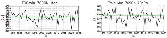
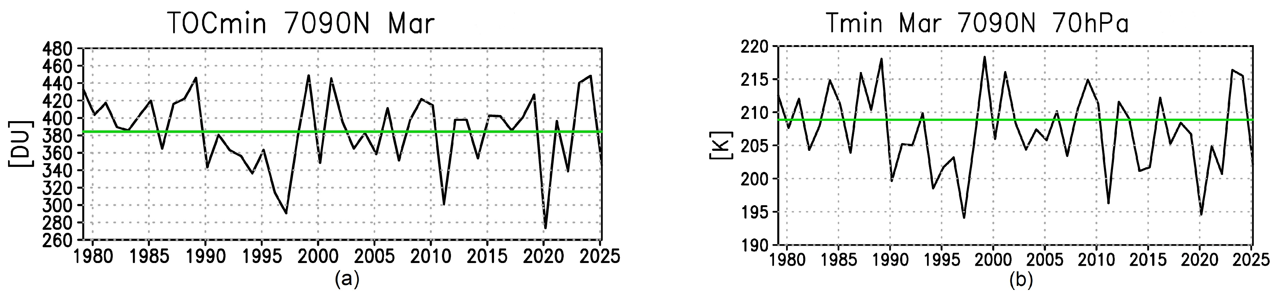
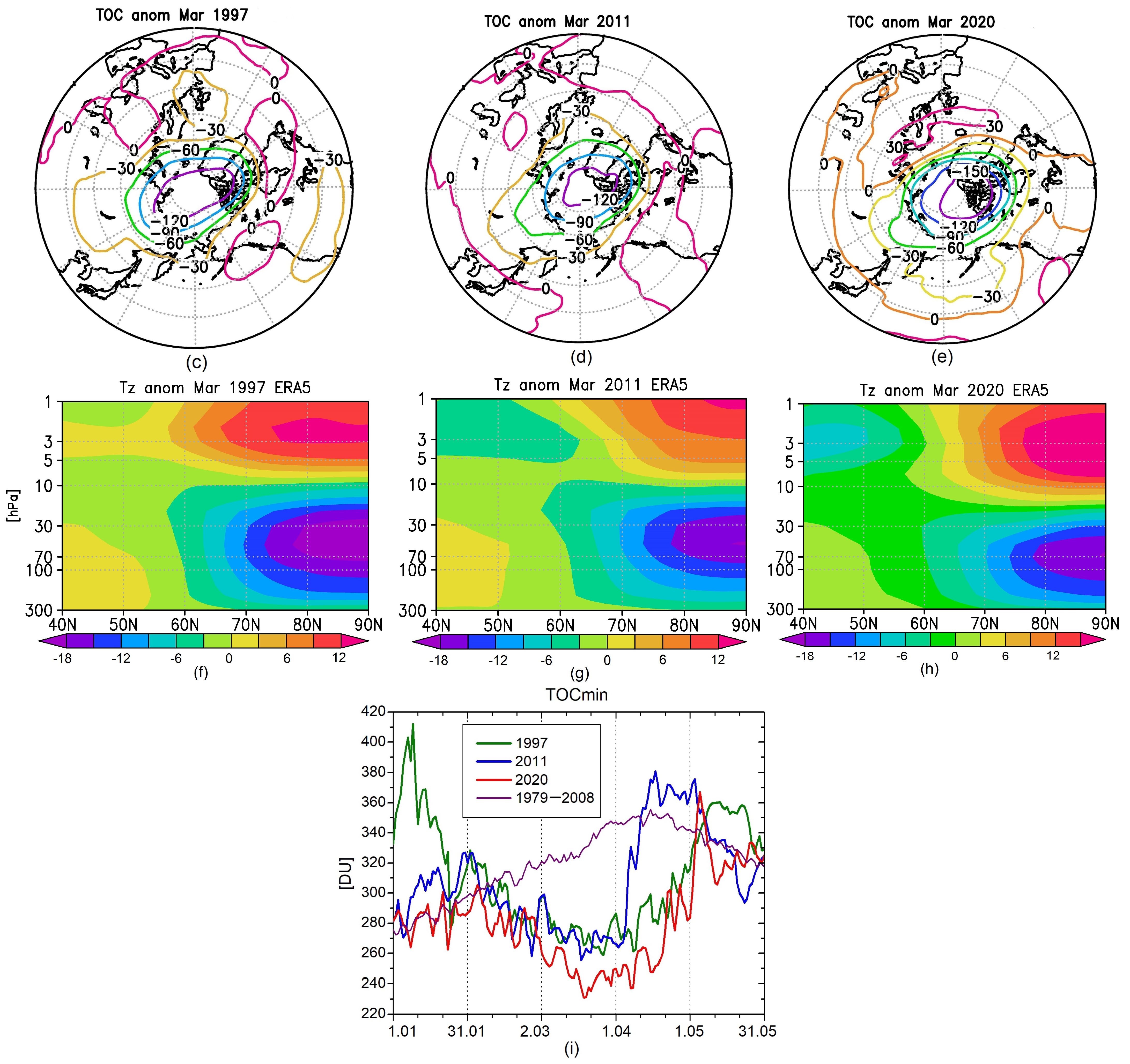
Between 1979 and 2025, the largest ozone anomalies were observed in the Arctic in March 1997, 2011, and the record-breaking event in March 2020. The minimum monthly mean TOC values at 70–90° N in these years were ~290 DU, ~300 DU, and ~280 DU, respectively, with the average minimum values over the period 1979–2008 being ~380 DU (Figure 1a). The minimum temperatures in the lower polar stratosphere at 70 hPa in these years were ~195 K (the threshold value for the formation of type I PSCs) with an average minimum of ~209 K (Figure 1b). The minimum lower stratospheric temperature and TOC minimum values in the polar region in March over 1979–2025 are positively correlated, with a correlation coefficient of 0.89 (Figure A1).
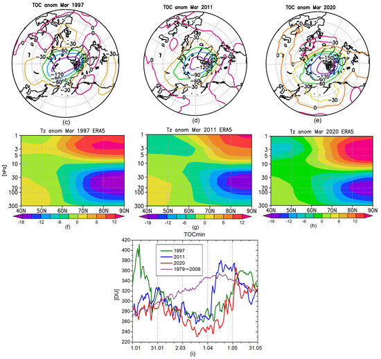
Figure 1.
(a) Minimum values of TOC and (b) temperature at pressure level 70 hPa at 70–90° N in March from 1979 to 2025. (c–e) TOC anomalies (DU) and (f–h) zonal mean temperature anomalies (K) in March 1997, 2011, 2020, respectively. (i) Minimum values of TOC at 70–90° N from 1 January to 31 May of 1997, 2011, 2020 and mean values over 1979–2008. Data: ERA5 reanalysis.
The largest TOC anomalies in the Arctic in these years were about −120 DU in March 1997 and 2011 and −150 DU in March 2020 (Figure 1c–e).
In these years the zonal mean wind velocity in March was 30–35 m/s higher than the 1979–2008 climatological values, with maximum values at pressure levels of 30–10 hPa in the 60–70° N region (Figure A1). The temperature of the Arctic lower stratosphere was 15–18 K lower than the climate mean values in the 70 hPa–30 hPa range (Figure 1f–h). In April the largest temperature anomalies were about −12 K in 1997 and 2020 (Figure A1e–g).
The minimum TOC at 70–90° N was about 230–260 DU in late March, with average minimum values of ~320–340 DU (Figure 1i).
3.2. Future Arctic Ozone Anomalies
As already mentioned, the greatest Arctic ozone depletion occurs in March under favorable dynamic conditions. The region where this depletion occurs (the ozone anomaly region) is characterized by minimal TOC values. SOCOLv3 simulations indicate that the high interannual variability in the Arctic stratosphere (which determines the strength of ozone depletion and thus the TOC minima) has persisted throughout the 21st century.
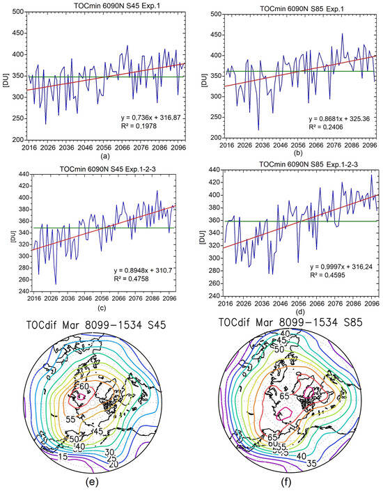
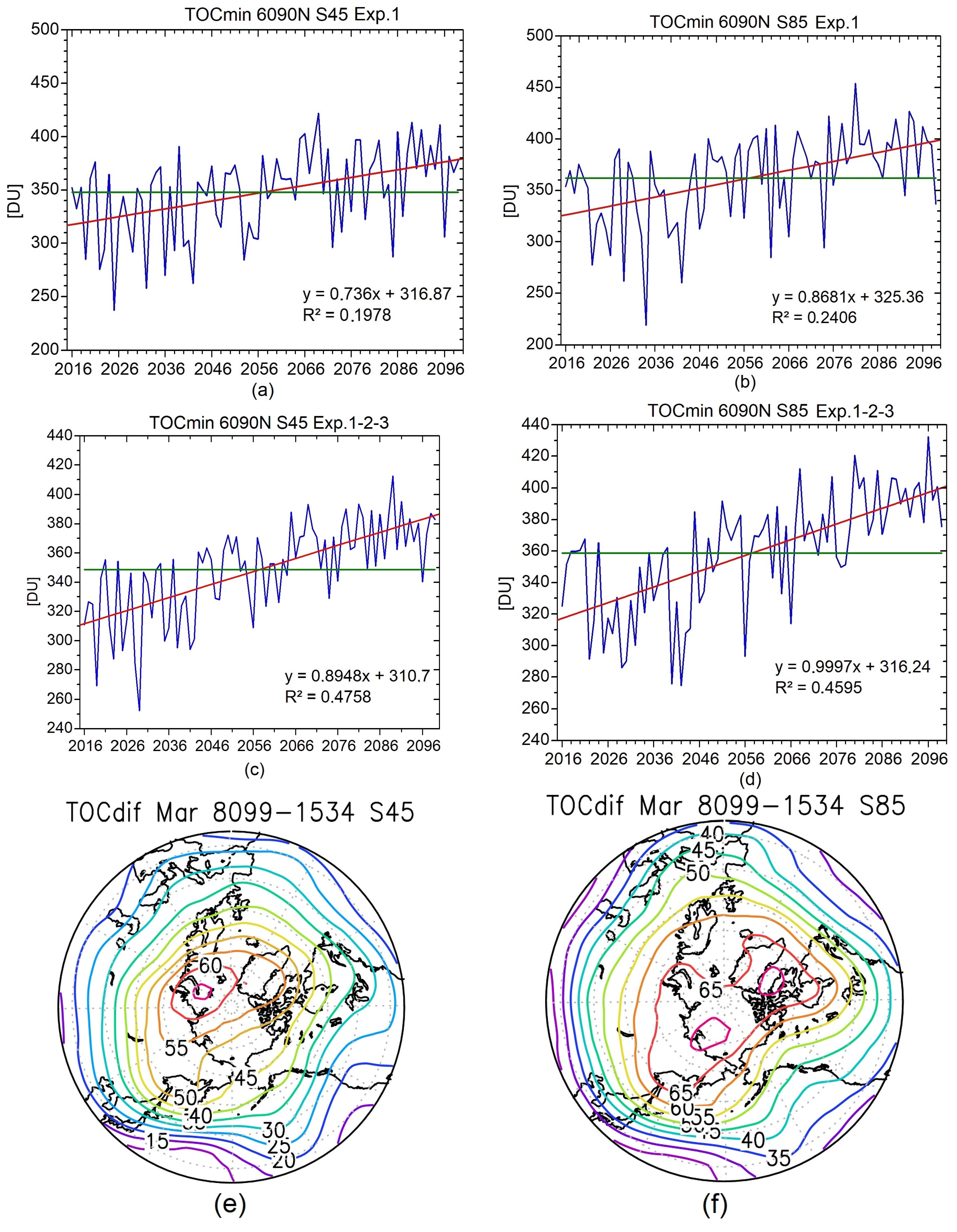
As an example, Figure 2 shows the variability in minimum TOC in March in the 60–90° N region for the first experiment and the ensemble means and differences between ensemble means of the averaged values over the last and first 20 years (2079–2099 and 2015–2035) of the analyzed period under the moderate and severe scenarios.
Figure 2.
(a,b) TOC minimum values at 60–90° N in March from 2016 to 2099 of the 1st experiment under moderate and severe scenarios and (c,d) ensemble mean values under the same scenarios. (e,f) Difference between TOC ensemble mean values in March averaged over the two periods 2080–2099 and 2015–2034 under moderate and severe scenarios respectively. For brevity, S45 and S85 in the plot title mean SSP2-4.5 and SSP5-8.5 scenarios respectively.
The results of the SOCOLv3 simulations indicate an increase in Arctic TOC in spring by the end of the 21st century under both scenarios, as follows:
- -
- Positive differences in TOC between the averaged values in March for the last and first 20 years of the analyzed period;
- -
- Positive trends in TOC in the polar region in March over the 21st century (these trends are significant according to Student’s t-test; p-values of these trends are less than 0.05 and are shown in Table A1);
- -
- Absence of comparable significant spring ozone anomalies in the second half of the 21st century compared with the first half.
Our results on the recovery of the ozone layer by the end of the 21st century are consistent with those of previous studies [2], for example, based on the analysis of calculations of version 4 of the CCM SOCOL with an interactive ocean block [33,49].
Further, changes in Arctic TOC during March–April were analyzed for the five selected coldest winter seasons with the lowest minimum TOCs in the polar region (60–90° N) in March (Table 1).
Table 1.
Selected coldest years with the lowest minimum TOC values in the polar region (60–90° N) in March for three experiments under moderate and severe scenarios.
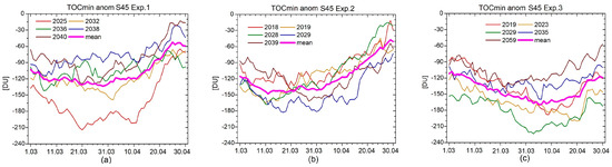
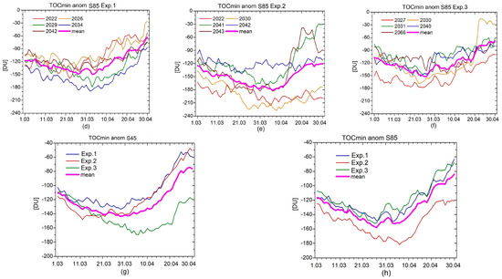
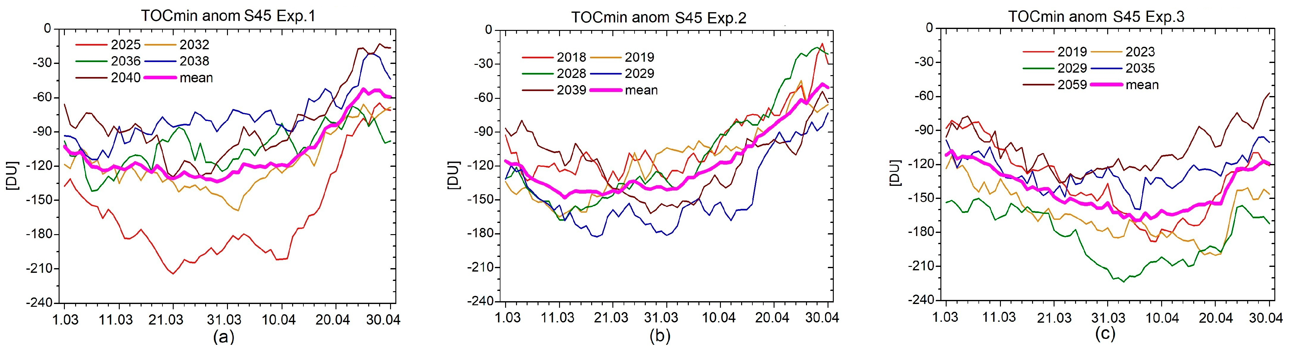
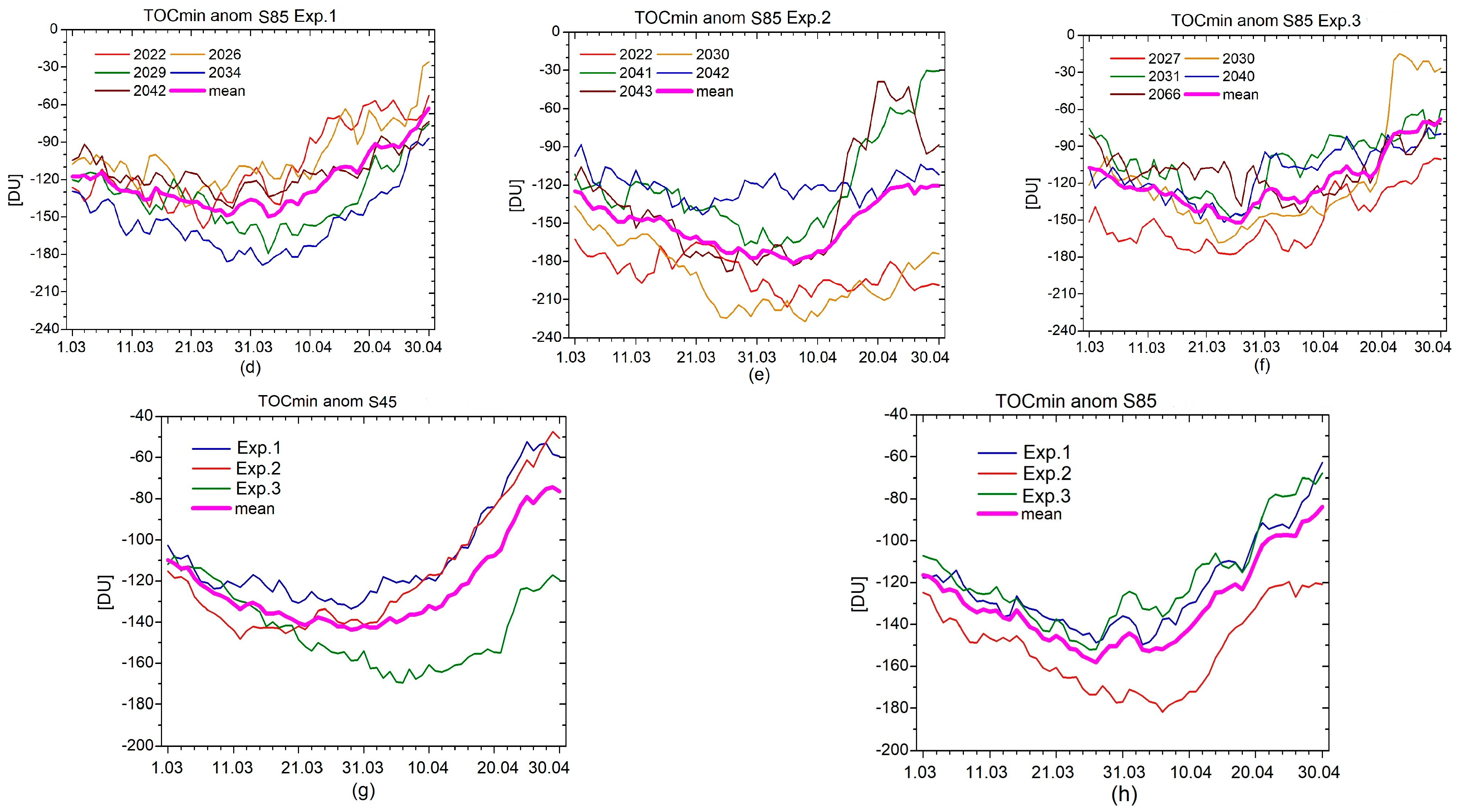
Figure 3a–f show anomalies in minimum TOC in the 60–90° N region in March–April relative to the mean values for the first half of each experiment from 2016 to 2058 for the moderate and severe scenarios. The average over the five selected coldest years for each ensemble calculation is presented (Figure 3g,h).
Figure 3.
Anomalies in minimum TOC over 60–90° N in March–April of the selected 5 “coldest” winters of three experiments (Exp. 1, Exp. 2, Exp. 3) for moderate (a,c,e) and severe (b,d,f) scenarios. Five “coldest” winter mean values are indicated as “mean”. (g,h) The mean values over the five selected coldest years for each ensemble calculation for moderate and severe scenarios. Ensemble mean values are indicated as “mean”.
In the moderate scenario, the lowest average values of TOC in March–April were found in the second experiment and, for the severe scenario, in the third. For these experiments, changes in the corresponding absolute TOC minimum in March–April are presented in Figure A2 and TOC minimum averaged over five “cold” winters in Figure A3. Under both scenarios, the lowest average TOC over the five coldest winters decrease to 200–220 DU in late March–early April (corresponding to anomaly values of around −180 DU). In some of the coldest seasons, the minimum TOC values drop to ~160 DU.
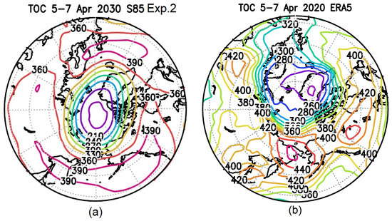
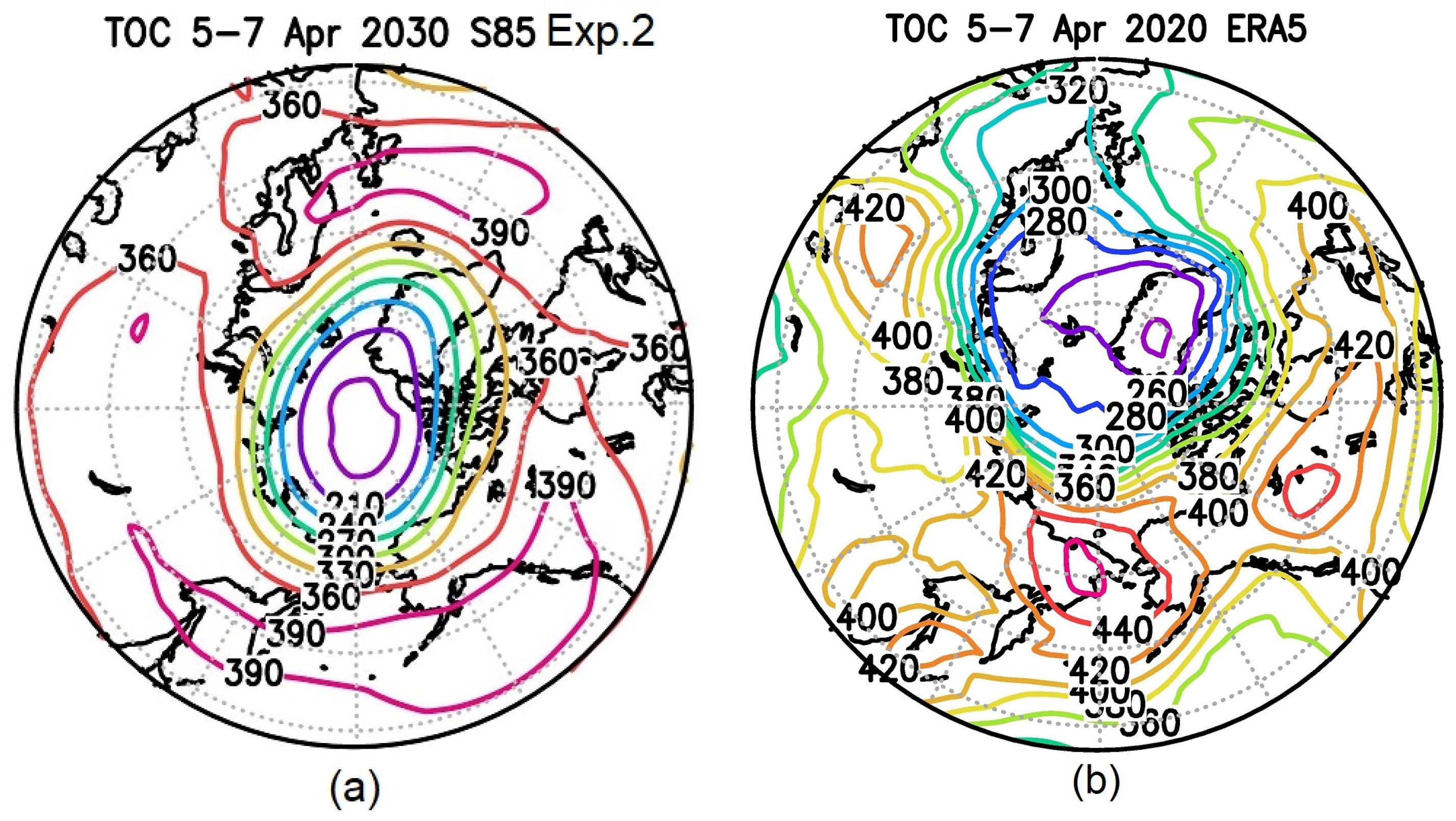
For example, Figure 4 shows the Arctic TOC from the second experiment of the severe scenario for 5–7 April of the 2030 model year and, for comparison, for the same dates in 2020 based on ERA5 reanalysis data. Minimum TOC values in the polar region dropped to 220 DU in late March–early April 2020.
Figure 4.
(a) Selected 3-day lowest TOC means over 5–7 April 2030 of the 2nd experiment under the severe scenario, (b) TOC 5–7 April 2020 (ERA5 reanalysis).
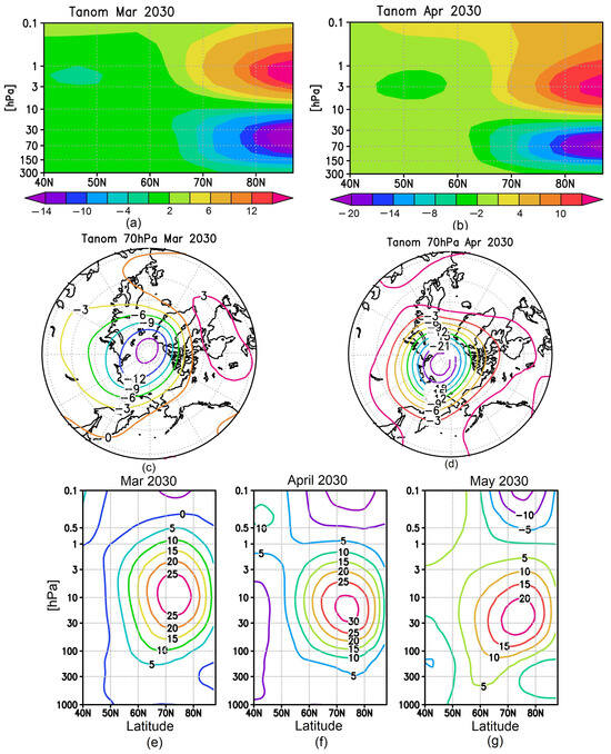
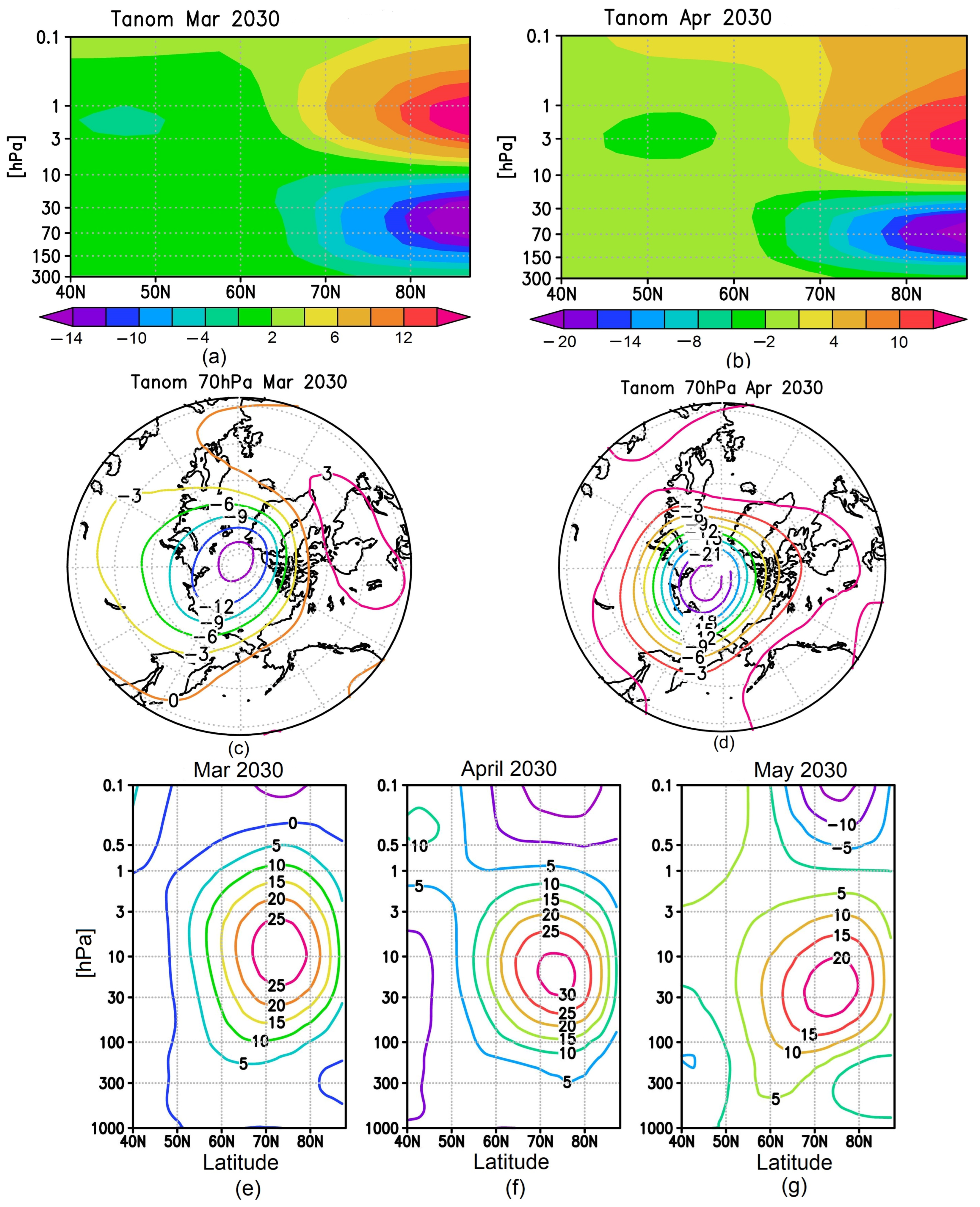
The lower polar stratosphere during this very cold winter is characterized by a low zonal mean temperature with negative anomalies below −16 K in March and −20 K in April 2030 (Figure 5a,b). At a pressure level of 70 hPa, the temperature anomalies are below −15 K and −24 K in these months, respectively (Figure 5c,d).
Figure 5.
(a,b) Monthly zonal mean temperature anomalies in March and April 2030 of 2nd experiment under severe scenario, (c,d) temperature anomalies at 70 hPa in March and April 2030, (e–g) zonal-mean zonal wind anomalies (m/s) in March, April and May 2030 (e–g). Anomalies are calculated respective to mean values over 2016–2058.
Model simulations show that the winter season of 2030 is characterized by increased zonal mean winds by ~25 m/s in March, ~30 m/s in April, and ~20 m/s in May in the region of the maximum near 30–10 hPa (Figure 5e–g). The spring breakup of the stratospheric circulation was detected in early June 2030, which is ~1.5 months later than the climatological means over 2016–2058: mid-April (Figure A4). Very low TOC values were revealed in the Arctic in the middle of May 2030, e.g., ~200–240 DU (Figure A5).
3.3. UVR Calculation
Changes in the ozone layer are among the primary factors affecting the surface UVR. During the record ozone depletion in late March and early April 2020, nearly 90% of ozone was depleted in the Arctic lower stratosphere [13], leading to a nearly 150% increase in surface UVR, according to ground-based measurements [50]. However, due to still-low solar zenith angles, the elevated UVR values remained at summer-season averages.
Enhanced UVR values were also recorded in the Arctic in spring 2011 [51]. The contribution of reduced TOC values to the increase in UVR, e.g., over Scandinavia, was ~50–60%, with the remainder being due to the cloudless sky.
The importance of anthropogenic ozone depletion for surface UVR during the present climate period was demonstrated through analysis of the CCM RSHU-INM simulations [52]. Other effects (solar activity, volcanic eruptions) have a significantly lesser impact.
Below are the estimates of the increase in UVR obtained using the MSU radiation model at 60° N and 70° N with an approximately two-week intervals for 25 March, 10 April, and 24 April for minimum TOC values and cloudless conditions at noon according to the SOCOLv3 calculations, as well as for the corresponding climatological values. The latitudinal belt 60–70° N includes several large northern cities: Murmansk, Arkhangelsk, Vorkuta, Norilsk, and Yakutsk (Russia), as well as Tromsø (Norway) and Anchorage (USA).
Results of UVR model calculations are presented further as the UV index (UVI)—internationally standardized measure of the erythemal UV radiation at the Earth’s surface in W/m2 divided by 0.025 W/m2 [53]. All UVI calculations used climatological monthly mean values of surface albedo and aerosol optical depth at a wavelength of 380 nm [40], available online (http://momsu.ru/uv/ accessed on 16 June 2026). TOC climate values are calculated using satellite TOMS data over 1979–2003. UVI estimates were obtained for cloudless and mean cloudy climatological conditions. Table 2 presents the simulated daily maximum UVI values on 25 March and 10 and 25 April at 60° N and 70° N under clear sky and typical cloud conditions.
Table 2.
The potential UV indices on 25 March and 10 and 25 April at 60° N and 70° N in clear sky (indicated as “Clear”) and typical cloud conditions (indicated as “Cloudy”). TOC climate values are indicated as “Standard”.
As might be expected, at the end of April, under cloudless conditions, UVR could increase by 100–140% (comparable to estimates for late March–early April 2020 [50]) to maximum UVI values of about 7.
According to the World Health Organization (WHO), for UVI values of 3–7, it is recommended to stay in the shade at midday, wear long-sleeved clothing, cover your head, use sunscreen, and protective glasses [54]. If the UVI exceed 8, it is additionally recommended to avoid outdoor activities during midday and seek shade. Skin type, age, and other health factors should be taken into account. Thus, the observed significant increase in UVI highlights the need for enhanced sun protection measures, especially given the body’s greater springtime sensitivity to increased UVR due to reduced melanin levels after winter [55].
Thus, our estimates show that, in the first half of the 21st century, in some winters, decreased TOC values near 200 DU are possible in the polar northern latitudes in March and even April. This leads to a significant increase in midday UVR under cloudless conditions or when taking into account its climatological values, compared to similar conditions but with climatological TOC. Notably the periods with reduced TOC and increased surface UVR persist for about two months.
4. Discussion and Conclusions
Future changes in the Arctic ozone layer will depend not only on ODS decline and GHG-induced stratospheric cooling but also on stratospheric circulation: a stronger, more-stable, and persistent stratospheric polar vortex will contribute to enhanced ozone destruction in some years.
Other factors that will affect the ozone layer in the Arctic include the expected strengthening of the meridional circulation, rising water vapor and nitric acid content in the lower stratosphere, and an enhanced role for sulfate aerosol with a temperature cooling due to an increase in the rate of heterogeneous reactions.
The strongest Arctic TOC anomalies in the late winter season may lead to enhanced surface UVR. However, when assessing possible future changes in UVR associated with periods of low TOC values, the main uncertainty is related to the difficulty in accounting for cloud conditions. The other uncertainties may be associated with changes in aerosol optical depth and reflectivity of the surface.
Overall, our analysis of three ensemble simulations of the CCM SOCOLv3, performed under the moderate and severe scenarios of GHGs (SSP2-4.5 and SSP5-8.5) and considering the expected decrease in ODS concentrations for 2016–2099, showed that
- (1)
- Despite severe chemical ozone destruction in the Arctic stratosphere for some years, all experiments show a positive TOC trend in the polar region 70–90° N in March.
- (2)
- High interannual variability in Arctic stratosphere circulation will remain throughout the 21st century.
- (3)
- In the first half of the 21st century, in the Arctic polar latitudes, on some days in March–April, TOC negative anomalies of 200 DU are possible relative to the 2016–2058 mean values. The minimum TOC values may drop below 220 DU (the accepted threshold of the ozone anomaly in Antarctica) to 160–180 DU.
- (4)
- Averaging over five seasons with the lowest March TOC values in the polar region of 70–90° N, mainly during the first half of the 21st century, and when averaging across three ensemble experiments, the most negative TOC anomalies up to −140 DU are possible at the end of March.
- (5)
- Estimates from the MSU radiation model indicate that, during years with the lowest TOC values in the second half of March and April, in regions with TOC near 200 DU and under clear midday sky, surface UV radiation can increase by about 100% to 140%. This corresponds to a UV index of 5–6, reaching up to 7 in April. In these conditions, sun protection measures, including use of sunscreen, are recommended.
Three interesting issues beyond the scope of this study are worth noting:
(1) Nonlinear interactions between upward-propagating planetary waves and stratospheric circulation govern the interannual variability in the stratospheric polar vortex. Favorable conditions for significant ozone depletion in the polar lower stratosphere—such as a strong, long-lasting, cold stratospheric vortex—develop due to weakened wave activity propagation from the troposphere. This weakening may be related to reduced wave formation in the troposphere or less favorable conditions for wave propagation in the stratosphere.
(2) Evaluation of the role of random processes and GHG-driven stratospheric circulation changes in the formation of Arctic ozone anomalies.
(3) Long-lasting impact of strong Arctic ozone anomalies: they can lead to increased surface UVR in the extratropical northern latitudes into summer [56]. Additionally, chemical ozone destruction in the Arctic stratosphere can contribute to the formation of short-term, but spatially extensive, ozone mini-holes such as those over northwestern Russia and Scandinavia in early March 2025 [7] and over European Russia in late May to early June 2025 [16].
Finally, this study’s estimates contribute to the discussion between [29] and [31] on the future of Arctic ozone: our results show the possibility for significant spring TOC anomalies in the Arctic in certain years, mainly in the first half of the 21st century, driven by favorable dynamic conditions under the expected recovery of the ozone layer.
Author Contributions
All authors made valuable contributions to the writing of the text, data analysis, and visualization of the results. Experimental setup, providing the data of chemistry–climate modeling, and interpretation of results, N.T., E.R., S.S. and P.V.; analysis of Arctic stratosphere dynamics and ozone layer changes, P.V. and V.G.; estimation of surface UV radiation changes, N.C. and P.V. All authors have read and agreed to the published version of the manuscript.
Funding
Chemistry–climate modeling and analysis of results were supported by the Russian Science Foundation (project #24-17-00230). The observed ozone anomalies in the Arctic were analyzed as part of a state assignment from the Ministry of Science and Higher Education to the Russian State Hydrometeorological University (project FSZU-2026-0003). Participation of ER in discussions of the experimental setup, interpretation of results, and writing of the text was supported by St. Petersburg State University (grant No. 124032000025-1). The interpretation of the results on UV changes by NC was partly supported by the MSU research project “Regional features of global climate change: diagnosis and mechanisms”.
Institutional Review Board Statement
Not applicable.
Informed Consent Statement
Not applicable.
Data Availability Statement
The data presented in this study are available on request from the corresponding author. The data are not publicly available due to privacy.
Acknowledgments
ERA5 reanalysis datasets by the Copernicus Climate Change Service. All plots in this study were made using the GridAnalysis and Display System (GrADS), which is a free software developed thanks to the NASA Advanced Information Systems Research Program. The authors are thankful to Sergey Kostrykin from Marchuk INM RAS for his useful remarks and suggestions and to two anonymous reviewers for their constructive and valuable comments.
Conflicts of Interest
The authors declare no conflicts of interest.
Abbreviations
The following abbreviations are used in this manuscript:
| CCM | Chemistry–climate model |
| GHGs | Greenhouse gases |
| ODSs | Ozone depleting substances |
| TOC | Total ozone content |
| PSCs | Polar stratospheric clouds |
| SSW | Sudden stratospheric warming |
| UVR | Ultraviolet solar radiation |
| UVI | Ultraviolet solar radiation index |
Appendix A
Figure A1.
(a) Minimum values of TOC and temperature at pressure level 70 hPa at 70–90° N in March from 1979 to 2025. For ease of comparison, the TOC minimum values were divided by 1.8. (b–d) Zonal-mean zonal wind anomalies (m/s) in March 1997, 2011, and 2020. (e–g) Zonal-mean temperature anomalies [K] in April 1997, 2011, 2020. Anomalies are calculated by subtracting the climate means over the period 1979–2008. Data: ERA5 reanalysis.
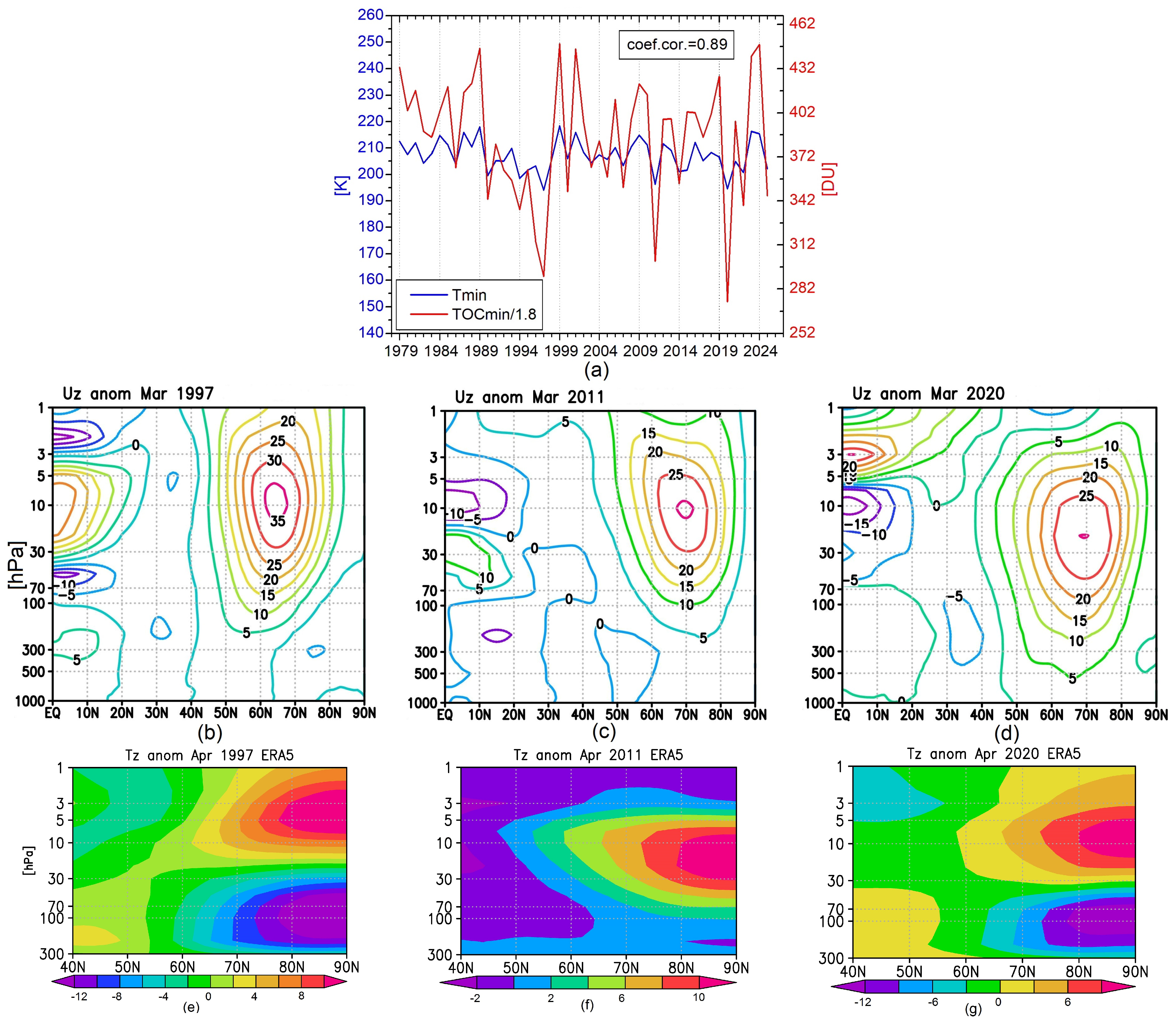
Figure A2.
Minimum TOC over 60–90° N in March–April of selected 5 “cold” winters of 3rd experiment under moderate scenario and 2nd experiment severe scenario (a,b). Five “cold” winters averaged values are indicated as “mean”.
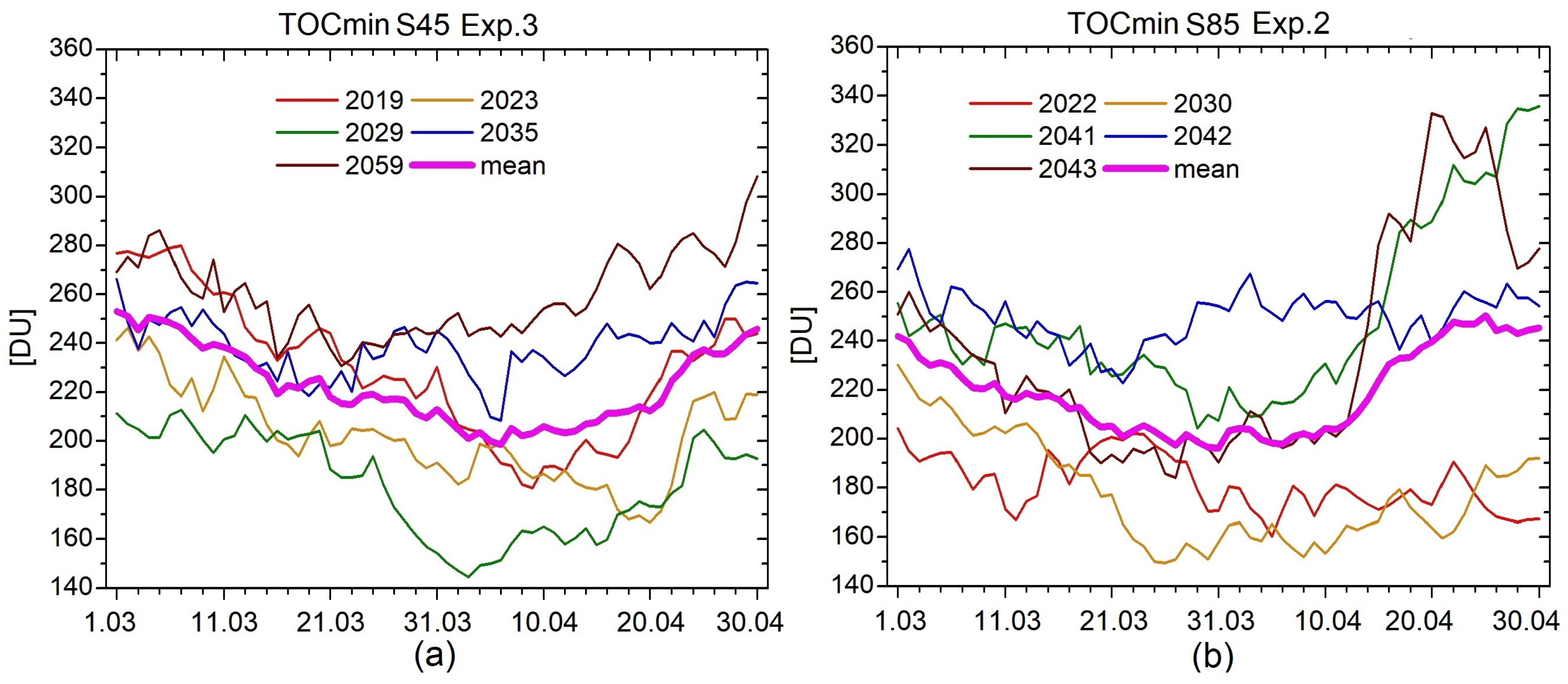
Figure A3.
Minimum TOC values in March-April averaged over 60–90° N and over five “cold” winters under moderate (a) and severe (b) scenarios respectively. Ensemble mean values over three experiments are indicated as “mean”.
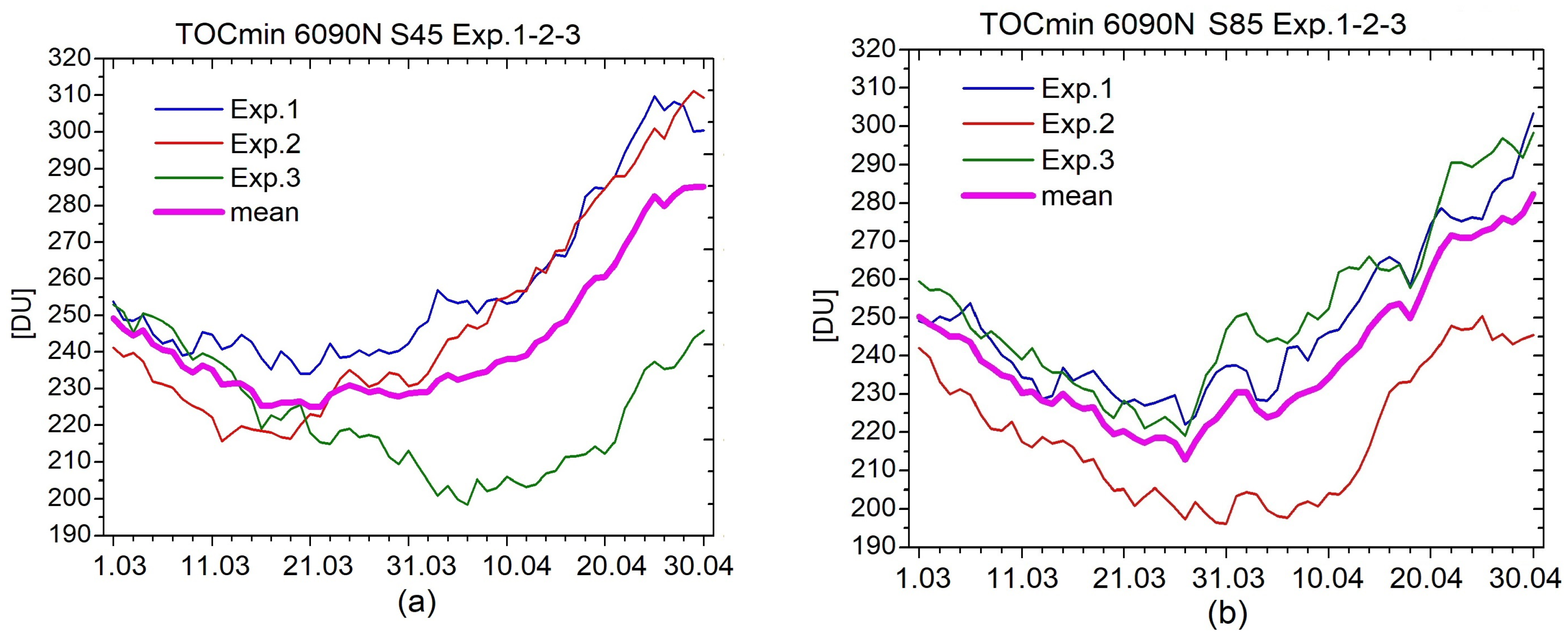
Figure A4.
Zonal-mean zonal wind (m/s) at 60° N from January to May averaged over 2016–2058 of the 2nd experiment under SSP5-8.5 scenario.
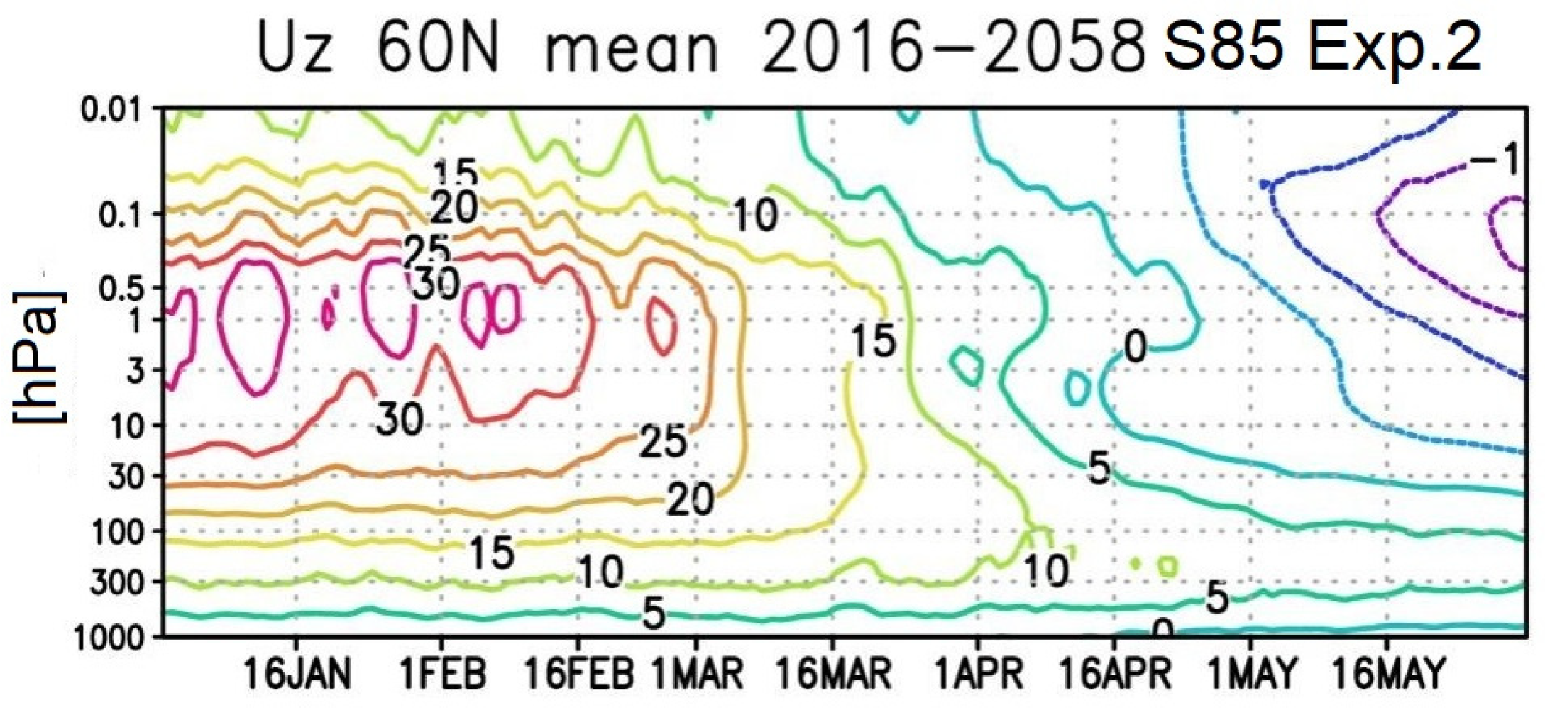
Figure A5.
(a,b) Selected 3-day lowest TOC means (DU) on 11–13 May and 15–17 May 2030 of the 2nd experiment under the severe SSP5-8.5 scenario.
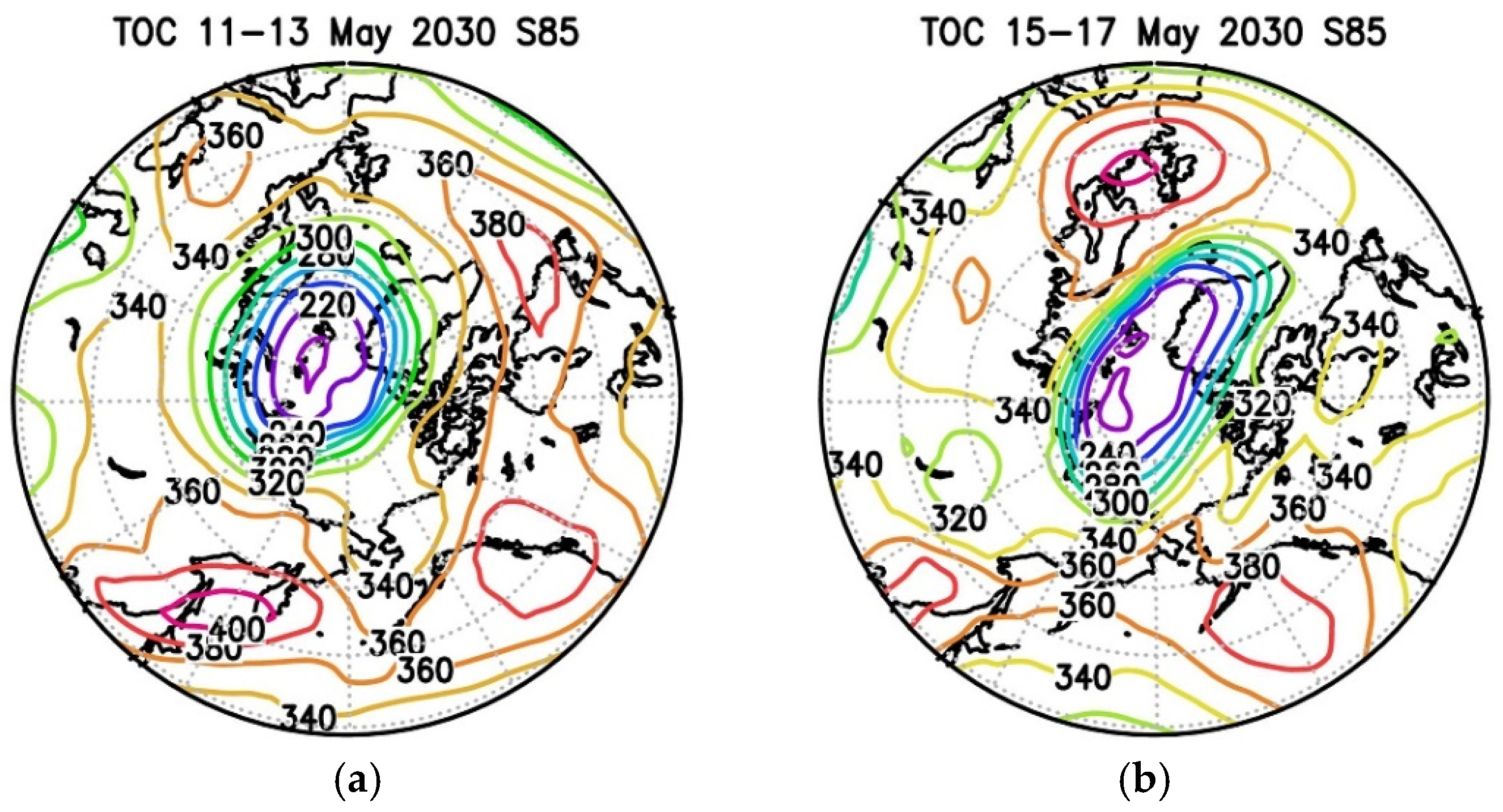
Table A1.
p-values of TOC trend in March over 2016–2099 for Exp. 1, Exp. 2, Exp. 3, and mean over these three experiments under the moderate and severe scenarios.
Surface UV Radiation and Cloudiness, Surface Albedo and Aerosol Optical Depth
Certainly, cloudiness is a very important factor for surface UVR. However, the aim of our study is the analysis of UVR changes due to low ozone anomalies in spring, and, hence, we focus on possible maximum UVR estimates calculated for clear sky conditions, which are the most dangerous for human health.
At present a short-term forecast is also often the estimated UV index for predicted cloud cover and for clear sky. See for instance, the UV index forecast in Germany:
https://www.bfs.de/EN/topics/opt/uv/index/forecast/forecast_node.html (accessed on 26 June 2026).
The main task of UV index forecast under clear sky is to warn a population of the maximum possible surface UV levels.
In our study we analyze UVR changes at noon due to low ozone values associated with the spring polar ozone anomalies over northern regions at latitudinal belt 60–70° N, which includes a number of large cities. Obviously, the cloud conditions may vary significantly over local points. Therefore, we show the possible maximum estimates calculated for clear sky conditions.
Our coldest March months were revealed in the model simulations in the first part of 21 century; therefore, for the nearest future (including record cold March 2030), the climate means of surface albedo and aerosol optical depth were used.
Also, the analysis of future variations in UV radiation due to other geophysical factors (surface albedo, aerosol loading) are vital but less important compared with that on ozone [57]. In addition, the quality of future projections of these factors should be studied thoroughly, and this is out of the scope of the paper.
Future research may be focused on the sensitivity analysis of possible ozone, cloudiness, surface albedo and aerosol optical depth changes over some regions or cities under conditions of long-term changes, for instance, in the middle or the late 21 century in comparison with the present.
References
- Baldwin, M.P.; Birner, T.; Brasseur, G.; Burrows, J.; Butchart, N.; Garcia, R.; Geller, M.; Gray, L.; Hamilton, K.; Harnik, N.; et al. 100 Years of progress in understanding the stratosphere and mesosphere. Meteorol. Monogr. 2019, 59, 27.1–27.62. [Google Scholar] [CrossRef] [Scilit]
- World Meteorological Organization (WMO). Scientific Assessment of Ozone Depletion: 2022; GAW Report No. 278; WMO: Geneva, Switzerland, 2022; 509p. [Google Scholar]
- Chipperfield, M.P.; Bekki, S.; Dhomse, S.; Harris, N.R.P.; Hassler, B.; Hossaini, R.; Steinbrecht, W.; Thiéblemont, R.; Weber, M. Detecting recovery of the stratospheric ozone layer. Nature 2017, 549, 211–218. [Google Scholar] [CrossRef] [Scilit] [PubMed]
- Morgenstern, O.; Braesicke, P.; Hurwitz, M.M.; O’COnnor, F.M.; Bushell, A.C.; Johnson, C.E.; Pyle, J.A. The World Avoided by the Montreal Protocol. Geophys. Res. Lett. 2008, 35, L16811. [Google Scholar] [CrossRef] [Scilit]
- Newman, P.A.; Oman, L.D.; Douglass, A.R.; Fleming, E.L.; Frith, S.M.; Hurwitz, M.M.; Kawa, S.R.; Jackman, C.H.; Krotkov, N.A.; Nash, E.R.; et al. What would have happened to the ozone layer if chlorofluorocarbons (CFCs) had not been regulated? Atmos. Chem. Phys. 2009, 9, 2113–2128. [Google Scholar] [CrossRef] [Scilit]
- Egorova, T.; Sedlacek, J.; Sukhodolov, T.; Karagodin-Doyennel, A.; Zilker, F.; Rozanov, E. Montreal Protocol’s impact on the ozone layer and climate. Atmos. Chem. Phys. 2023, 23, 5135–5147. [Google Scholar] [CrossRef] [Scilit]
- Vargin, P.; Smyshlyaev, S.; Guryanov, V.; Chubarova, N.; Ionov, D.; Bankova, T.; Ivanova, N.; Solomatnikova, A. A Study of the Low-Ozone Episode over Scandinavia and Northwestern Russia in March 2025. Atmosphere 2025, 16, 1033. [Google Scholar] [CrossRef] [Scilit]
- Manney, G.L.; Santee, M.L.; Rex, M.; Livesey, N.J.; Pitts, M.C.; Veefkind, P.; Nash, E.R.; Wohltmann, I.; Lehmann, R.; Froidevaux, L.; et al. Unprecedented Arctic ozone loss in 2011. Nature 2011, 478, 469–475. [Google Scholar] [CrossRef] [Scilit] [PubMed]
- Lawrence, Z.D.; Perlwitz, J.; Butler, A.H.; Manney, G.L.; Newman, P.A.; Lee, S.H.; Nash, E.R. The remarkably strong arctic stratospheric polar vortex of winter 2020: Links to record-breaking arctic oscillation and ozone loss. J. Geophys. Res. Atmos. 2020, 125, e2020JD033271. [Google Scholar] [CrossRef] [Scilit]
- Manney, G.L.; Livesey, N.J.; Santee, M.L.; Froidevaux, L.; Lambert, A.; Lawrence, Z.D.; Millán, L.F.; Neu, J.L.; Read, W.G.; Schwartz, M.J.; et al. Record—Low Arctic stratospheric ozone in 2020: MLS observations of chemical processes and comparisons with previous extreme winters. Geophys. Res. Lett. 2020, 47, e2020GL089063. [Google Scholar] [CrossRef] [Scilit]
- Smyshlyaev, S.; Vargin, P.; Motsakov, M. Numerical modeling of ozone loss in the exceptional Arctic stratosphere winter-spring of 2020. Atmosphere 2021, 12, 1470. [Google Scholar] [CrossRef] [Scilit]
- Tsvetkova, N.D.; Vargin, P.N.; Lukyanov, A.N.; Kiryushov, B.M.; Yushkov, V.A.; Khattatov, V.U. Investigation of chemistry ozone destruction and dynamical processes in Arctic stratosphere in winter 2019–2020. Russ. Meteor. Hydrol. 2021, 46, 606–615. [Google Scholar] [CrossRef] [Scilit]
- Wohltmann, I.; von der Gathen, P.; Lehmann, R.; Maturilli, M.; Deckelmann, H.; Manney, G.L.; Davies, J.; Tarasick, D.; Jepsen, N.; Kivi, R.; et al. Near-complete local reduction of Arctic stratospheric ozone by severe chemical loss in spring 2020. Geophys. Res. Lett. 2020, 47, e2020GL089547. [Google Scholar] [CrossRef] [Scilit]
- Dameris, M.; Loyola, D.G.; Nützel, M.; Coldewey-Egbers, M.; Lerot, C.; Romahn, F.; van Roozendael, M. Record low ozone values over the Arctic in boreal spring 2020. Atmos. Chem. Phys. 2021, 21, 617–633. [Google Scholar] [CrossRef] [Scilit]
- Vargin, P.; Koval, A.; Perminov, V.; Guryanov, V.; Tsvetkova, N.; Korshunov, V.; Rozanov, E.; Wei, K. Troposphere–Stratosphere–Mesosphere Coupling and Ozone Response to Arctic Stratospheric Variability during the 2024–2025 Winter Season. Adv. Atmos. Sci. 2026. [Google Scholar] [CrossRef] [Scilit]
- Vargin, P.; Fomin, B.; Chubarova, N.; Tsvetkova, N.D.; Sumerova, K.A.; Bankova, T.V.; Khattatov, V.U.; Sokolov, A.V.; Rozanov, E.V. A study of the formation of the ozone “mini-hole” over the European territory of Russia in late May—Early June 2025 and its impact on ground-level UV radiation. Russ. Meteor. Hydrol. 2026; accepted.
- Kessenich, H.; Seppälä, A.; Rodger, C. Potential drivers of the recent large Antarctic ozone holes. Nat. Commun. 2023, 14, 7259. [Google Scholar] [CrossRef] [Scilit] [PubMed]
- Yook, S.; Thompson, D.; Solomon, S. Climate impacts and potential drivers of the unprecedented Antarctic ozone holes of 2020 and 2021. Geophys. Res. Lett. 2022, 49, e2022GL098064. [Google Scholar] [CrossRef] [Scilit]
- Friedel, M.; Chiodo, G.; Stenke, A.; Domeisen, D.I.; Fueglistaler, S.; Anet, J.G.; Peter, T. Springtime arctic ozone depletion forces northern hemisphere climate anomalies. Nat. Geosci. 2022, 15, 541–547. [Google Scholar] [CrossRef] [Scilit]
- Pommereau, J.-P.; Goutail, F.; Pazmino, A.; Lefèvre, F.; Chipperfield, M.P.; Feng, W.; Van Roozendael, M.; Jepsen, N.; Hansen, G.; Kivi, R.; et al. Recent Arctic ozone depletion: Is there an impact of climate change? Comptes Rendus Géosci. 2018, 350, 347–353. [Google Scholar] [CrossRef] [Scilit]
- Friedel, M.; Chiodo, G.; Sukhodolov, T.; Keeble, J.; Peter, T.; Seeber, S.; Stenke, A.; Akiyoshi, H.; Rozanov, E.; Plummer, D.; et al. Weakening of springtime Arctic ozone depletion with climate change. Atmos. Chem. Phys. 2023, 23, 10235–10254. [Google Scholar] [CrossRef] [Scilit]
- Langematz, U.; Meul, S.; Grunow, K.; Romanowsky, E.; Oberländer, S.; Abalichin, J.; Kubin, A. Future Arctic temperature and ozone: The role of stratospheric composition changes. J. Geophys. Res. Atmos. 2014, 119, 2092–2112. [Google Scholar] [CrossRef] [Scilit]
- Bednarz, E.; Maycock, A.; Abraham, L.; Braesicke, P.; Dessens, O.; Pyle, J. Future Arctic ozone recovery: The importance of chemistry and dynamics. Atmos. Chem. Phys. 2016, 16, 12159–12176. [Google Scholar] [CrossRef] [Scilit]
- Watanabe, S.; Sudo, K.; Nagashima, T.; Takemura, T.; Kawase, H.; Nozawa, T. Future projections of surface UV-B in a changing climate. J. Geophys. Res. 2011, 116, D16118. [Google Scholar] [CrossRef] [Scilit]
- Fountoulakis, I.; Bais, A.F.; Tourpali, K.; Fragkos, K.; Misios, S. Projected changes in solar UV radiation in the Arctic and sub-Arctic Oceans: Effects from changes in reflectivity, ice transmittance, clouds, and ozone. J. Geophys. Res. Atmos. 2014, 119, 8073–8090. [Google Scholar] [CrossRef] [Scilit]
- Pastukhova, A.S.; Chubarova, N.E.; Zhdanova, Y.Y.; Galin, V.Y.; Smyshlyaev, S.P. Numerical Simulation of Variations in Ozone Content, Erythemal Ultraviolet Radiation, and Ultraviolet Resources over Northern Eurasia in the 21st Century. Izv. Atmos. Ocean. Phys. 2019, 55, 242–250. [Google Scholar] [CrossRef] [Scilit]
- Yamamoto, A.L.C.; Corrêa, M.d.P.; Torres, R.R.; Martins, F.B.; Godin-Beekmann, S. Projected changes in ultraviolet index and UV doses over the twenty-first century: Impacts of ozone and aerosols from CMIP6. Photochem. Photobiol. Sci. 2024, 23, 1279–1294. [Google Scholar] [CrossRef] [Scilit] [PubMed]
- Zubov, V.; Rozanov, E.; Egorova, T. Projection of the UV Radiation for Vitamin D Production Changes Between 2015–2024 and 2090–2099 Periods. Atmosphere 2025, 16, 686. [Google Scholar] [CrossRef] [Scilit]
- von der Gathen, P.; Kivi, R.; Wohltmann, I.; Salawitch, R.J.; Rex, M. Climate change favours large seasonal loss of Arctic ozone. Nat. Commun. 2021, 12, 3886. [Google Scholar] [CrossRef] [Scilit] [PubMed]
- Rex, M.; Salawitch, R.J.; Deckelmann, H.; von der Gathen, P.; Harris, N.R.P.; Chipperfield, M.P.; Naujokat, B.; Reimer, E.; Allaart, M.; Andersen, S.B.; et al. Arctic winter 2005: Implications for stratospheric ozone loss and climate change. Geophys. Res. Lett. 2006, 33, L23808. [Google Scholar] [CrossRef] [Scilit]
- Polvani, L.M.; Keeble, J.; Banerjee, A.; Checa-Garcia, R.; Chiodo, G.; Rieder, H.E.; Rosenlof, K.H. No evidence of worsening arctic springtime ozone losses over the 21st century. Nat. Commun. 2023, 14, 1608. [Google Scholar] [CrossRef] [Scilit] [PubMed]
- Vargin, P.; Kostrykin, S.; Volodin, E.; Pogoreltsev, A.; Wei, K. Arctic Stratosphere Circulation Changes in the 21st Century in Simulations of INM CM5. Atmosphere 2022, 13, 25. [Google Scholar] [CrossRef] [Scilit]
- Vargin, P.; Kostrykin, S.; Koval, A.; Rozanov, E.; Egorova, T.; Smyshlyaev, S.; Tsvetkova, N. Arctic stratosphere changes in the 21st century in the Earth system model SOCOLv4. Front. Earth Sci. 2023, 11, 1214418. [Google Scholar] [CrossRef] [Scilit]
- Stenke, A.; Schraner, M.; Rozanov, E.; Egorova, T.; Luo, B.; Peter, T. The SOCOL version 3.0 chemistry–climate model: Description, evaluation, and implications from an advanced transport algorithm. Geosci. Model Dev. 2013, 6, 1407–1427. [Google Scholar] [CrossRef] [Scilit]
- Riahi, K.; Van Vuuren, D.P.; Kriegler, E.; Edmonds, J.; O’Neill, B.C.; Fujimori, S.; Bauer, N.; Calvin, K.; Dellink, R.; Fricko, O.; et al. The Shared Socioeconomic Pathways and their energy, land use, and greenhouse gas emissions implications: An overview. Glob. Environ. Change 2017, 42, 153–168. [Google Scholar] [CrossRef] [Scilit]
- Zhao, S.; Yu, Y.; Lin, P.; Liu, H.; He, B.; Bao, Q.; Guo, Y.; Hua, L.; Chen, K.; Wang, X. Datasets for the CMIP6 scenario model intercomparison project (ScenarioMIP) simulations with the coupled model CAS FGOALS-f3-L. Adv. Atmos. Sci. 2020, 38, 329–339. [Google Scholar] [CrossRef] [Scilit]
- Plummer, D.A.; Nagashima, T.; Tilmes, S.; Archibald, A.; Chiodo, G.; Fadnavis, S.; Garny, H.; Josse, B.; Kim, J.; Lamarque, F.; et al. CCMI—2022: A new set of Chemistry—Climate Model Initiative (CCMI) community simulations to update the assessment of models and support upcoming ozone assessment activities. SPARC Newsl. 2021, 57, 22–30. [Google Scholar]
- Marsh, D.R.; Mills, M.J.; Kinnison, D.E.; Lamarque, J.-F.; Calvo, N.; Polvani, L.M. Climate Change from 1850 to 2005 Simulated in CESM1(WACCM). J. Clim. 2013, 26, 7372–7391. [Google Scholar] [CrossRef] [Scilit]
- Steiner, M.; Luo, B.; Peter, T.; Pitts, M.C.; Stenke, A. Evaluation of polar stratospheric clouds in the global chemistry–climate model SOCOLv3.1 by comparison with CALIPSO spaceborne lidar measurements. Geosci. Model Dev. 2021, 14, 935–959. [Google Scholar] [CrossRef] [Scilit]
- Chubarova, N.; Zhdanova, Y. Ultraviolet resources over Northern Eurasia. J. Photochem. Photobiol. B Biol. 2013, 127, 38–51. [Google Scholar] [CrossRef] [Scilit]
- Chubarova, N.; Zhdanova, Y.; Nezval, Y. A new parameterization of the UV irradiance altitude dependence for clear-sky conditions and its application in the on-line UV tool over Northern Eurasia. Atmos. Chem. Phys. 2016, 16, 11867–11881. [Google Scholar] [CrossRef] [Scilit]
- Ardra, D.; Kuttippurath, J.; Roy, R.; Kumar, P.; Raj, S.; Müller, R.; Feng, W. The Unprecedented Ozone Loss in the Arctic Winter and Spring of 2010/2011 and 2019/2020. ACS Earth Space Chem. 2022, 6, 683–693. [Google Scholar] [CrossRef] [Scilit]
- Baldwin, M.P.; Ayarzagüena, B.; Birner, T.; Butchart, N.; Butler, A.H.; Charlton-Perez, A.J.; Domeisen, D.I.V.; Garfinkel, C.I.; Garny, H.; Gerber, E.P.; et al. Sudden stratospheric warmings. Rev. Geophys. 2021, 59, e2020RG000708. [Google Scholar] [CrossRef] [Scilit]
- Matsuno, T. A dynamical model of the stratospheric sudden warming. J. Atmos. Sci. 1971, 28, 1479–1494. [Google Scholar] [CrossRef] [Scilit]
- Pogoreltsev, A. Generation of normal atmospheric modes by stratospheric vacillations. Izv. Atmos. Ocean. Phys. 2007, 43, 423–435. [Google Scholar] [CrossRef] [Scilit]
- de la Cámara, A.; Albers, J.R.; Birner, T.; Garcia, R.R.; Hitchcock, P.; Kinnison, D.E.; Smith, A.K. Sensitivity of sudden stratospheric warmings to previous stratospheric conditions. J. Atmos. Sci. 2017, 74, 2857–2877. [Google Scholar] [CrossRef] [Scilit]
- Newman, P.A.; Lait, L.R.; Kramarova, N.A.; Coy, L.; Frith, S.M.; Oman, L.D.; Dhomse, S.S. Record high march 2024 Arctic total column ozone. Geophys. Res. Lett. 2024, 51, e2024GL110924. [Google Scholar] [CrossRef] [Scilit]
- Hersbach, H.; Bell, B.; Berrisford, P.; Hirahara, S.; Horányi, A.; Muñoz-Sabater, J.; Nicolas, J.; Peubey, C.; Radu, R.; Schepers, D.; et al. The ERA5 global reanalysis. Q. J. R. Meteorol. Soc. 2020, 146, 1999–2049. [Google Scholar] [CrossRef] [Scilit]
- Karagodin-Doyennel, A.; Rozanov, E.; Sukhodolov, T.; Egorova, T.; Sedlacek, J.; Peter, T. The future ozone trends in changing climate simulated with SOCOLv4. EGUsphere 2023, 23, 4801–4817. [Google Scholar] [CrossRef] [Scilit]
- Bernhard, G.H.; Fioletov, V.E.; Grooß, J.; Ialongo, I.; Johnsen, B.; Lakkala, K.; Manney, G.L.; Müller, R.; Svendby, T. Record-Breaking Increases in Arctic Solar Ultraviolet Radiation Caused by Exceptionally Large Ozone Depletion in 2020. Geophys. Res. Lett. 2020, 47, e2020GL090844. [Google Scholar] [CrossRef] [Scilit] [PubMed]
- Bernhard, G.; Dahlback, A.; Fioletov, V.; Heikkilä, A.; Johnsen, B.; Koskela, T.; Lakkala, K.; Svendby, T. High levels of ultraviolet radiation observed by ground-based instruments below the 2011 Arctic ozone hole. Atmos. Chem. Phys. 2013, 13, 10573–10590. [Google Scholar] [CrossRef] [Scilit]
- Chubarova, N.E.; Pastukhova, A.S.; Zhdanova, E.Y.; Volpert, E.V.; Smyshlyaev, S.P.; Galin, V.Y. Effects of Ozone and Clouds on Temporal Variability of Surface UV Radiation and UV Resources over Northern Eurasia Derived from Measurements and Modeling. Atmosphere 2020, 11, 59. [Google Scholar] [CrossRef] [Scilit]
- Vanicek, K.; Frei, T.; Litynska, Z.; Schmalwieser, A. UV-Index for the Public; COST-713 Action; European Union: Brussels, Belgium, 2000; 27p. [Google Scholar]
- World Health Organization (WHO). Available online: https://www.who.int/news-room/questions-and-answers/item/radiation-the-ultraviolet-(uv)-index (accessed on 16 May 2026).
- Czerwińska, A.E.; Krzyścin, J.W. Climatological aspects of the increase of the skin cancer (melanoma) incidence rate in Europe. Int. J. Climatol. 2019, 40, 3196–3207. [Google Scholar] [CrossRef] [Scilit]
- Karpechko, A.Y.; Backman, L.; Thölix, L.; Ialongo, I.; Andersson, M.; Fioletov, V.; Heikkilä, A.; Johnsen, B.; Koskela, T.; Kyrölä, E.; et al. The link between springtime total ozone and summer UV radiation in Northern Hemisphere extratropics. J. Geophys. Res. 2013, 118, 8649–8661. [Google Scholar] [CrossRef] [Scilit]
- Chubarova, N.E. UV variability in Moscow according to long-term UV measurements and reconstruction model. Atmos. Chem. Phys. 2008, 8, 3025–3031. [Google Scholar] [CrossRef] [Scilit]

Disclaimer/Publisher’s Note: The statements, opinions and data contained in all publications are solely those of the individual author(s) and contributor(s) and not of MDPI and/or the editor(s). MDPI and/or the editor(s) disclaim responsibility for any injury to people or property resulting from any ideas, methods, instructions or products referred to in the content. |
© 2026 by the authors. Licensee MDPI, Basel, Switzerland. This article is an open access article distributed under the terms and conditions of the Creative Commons Attribution (CC BY) license.