


Abstract
Street-level concentrations of nitrogen dioxide (NO2) and fine particulate matter (PM2.5) pose serious public health risks in European cities, yet accurate multi-year prediction at traffic-dominated sites remains challenging. This study applies XGBoost (XGB) and Random Forest (RF) to predict hourly NO2 and daily PM2.5 at two street monitoring sites in Copenhagen, Denmark, trained on 17 years of observational data and evaluated on two independent years. Three-dimensional variational assimilation (3D-Var) and the Extended Kalman Filter (EKF) are then applied as post-processing corrections to the ML predictions using co-located observations. XGB achieved RMSE values of 9.5 and 7.4 µg/m3 for HCAB and JGTV NO2, respectively, in the 2018 test year. Both DA methods improved substantially on the ML baseline, with 3D-Var reducing NO2 RMSE by up to 57% and spike event RMSE by up to 51%. EKF achieved near-complete elimination of systematic bias across all configurations. The framework is computationally lightweight and can be applied to any deterministic model prediction at a monitoring station, including outputs from physics- and chemistry-based dispersion models. Overall, the findings show a practical way to improve street-level air quality prediction, with direct relevance for operational forecasting and public health protection.
1. Introduction
Air pollution remains one of the leading environmental threats to human health in Europe. Despite gradual improvements through regulatory measures, the European Union’s revised Air Quality Directive (2024/2881) confirms that millions of citizens continue to be exposed to pollutant levels exceeding safe thresholds [1,2]. Fine particulate matter (PM2.5) and nitrogen dioxide (NO2) are among the most harmful pollutants, associated with serious conditions such as heart disease [3], lung cancer [4], and stroke [5]. In 2022, long-term exposure to PM2.5 accounted for approximately 239,000 premature deaths in the EU [6], while NO2 remained a significant contributor to respiratory and cardiovascular mortality [1]. These figures highlight the urgent need for accurate prediction and forecasting systems to inform policy and protect public health.
Street-level air pollution is a particular concern in urban areas, where people live, work, and commute in close proximity to traffic. Road transport is the dominant source of NO2 and PM2.5 at urban street sites, driving sharp concentration gradients within individual city blocks and creating exposure conditions that differ markedly from urban background levels [7,8]. Predicting these concentrations accurately at street scale is essential for early warning systems, urban planning, and emission-reduction strategies, and it is a prerequisite for evidence-based policy interventions aimed at reducing human exposure and protecting vulnerable populations. Yet it remains one of the harder problems in applied air quality modelling, because street environments respond rapidly to traffic dynamics, local meteorology, and the physical geometry of the surrounding buildings [9,10].
Traditional physics- and chemistry-based dispersion models have long served as the backbone of urban air quality assessment. These models simulate pollutant transport and chemistry using well-established physical principles, but they depend on assumptions that may not reflect real-world conditions at fine spatial scales. The Danish AirGIS model, for example, treats emissions as homogeneously distributed along road segments [11], which can introduce uncertainties in concentration estimates at individual sites [12]. Although fixed-site monitoring stations do not provide the spatial coverage of model grids, they deliver high-quality, consistent measurements that remain indispensable for exposure assessment and model evaluation.
Machine learning (ML) methods have emerged as a practical alternative for predicting NO2 and PM2.5 concentrations, because they can process large observational datasets and identify complex, non-linear relationships between pollutant concentrations and their drivers [13,14,15]. Among these, Extreme Gradient Boosting (XGB) and Random Forest (RF) have become the most widely applied tree-based ensemble methods in air quality modelling.
XGB builds an ensemble of decision trees sequentially, using regularisation and gradient optimisation to minimise prediction error and reduce overfitting [16,17]. A 2025 study estimated ground-level NO2 over megacities using Sentinel-5P satellite data combined with ground monitoring stations; XGB outperformed other ML models, achieving RMSE values between 19.6 and 20.1 µg/m3 [18].
RF combines multiple independently grown decision trees and has demonstrated strong performance on tabular environmental data, particularly where non-linear interactions between traffic, meteorology, and local context are prominent [19,20]. A nationwide Swedish study applied RF to estimate daily PM2.5, PM10, and NO2 at 1 km resolution, explaining 64–78% of variance in held-out observations [21]. While both models show consistent strengths, the relative advantage of XGB over RF, and under which conditions each performs better, remains dataset- and context-dependent, particularly at traffic-dominated street sites [22,23].
Most published ML studies have focused on relatively short prediction horizons [24,25]. This is partly because uncertainty compounds over longer horizons, and partly because few datasets span the multi-year periods needed to evaluate long-term and seasonal performance. Evaluating ML approaches over decadal timescales, covering multiple annual cycles, seasonal transitions, and changes in the emission environment, remains an important but underexplored challenge.
Data assimilation (DA) offers a principled framework for reducing such uncertainty by incorporating observational information directly into model estimates. DA methods minimise the difference between model predictions and observations in a statistically optimal way, improving both short-term accuracy and the physical consistency of forecasts [26,27]. Three-dimensional variational assimilation (3D-Var) achieves this by minimising a cost function that balances background model error against observational error, producing an analysis field that is closer to the observed state than the unadjusted model alone [28,29]. The Extended Kalman Filter (EKF) takes a sequential approach, updating model estimates at each time step using a linearised error propagation, which makes it well-suited to tracking evolving pollutant concentrations over time [30,31].
The combination of ML and DA is an active area of development in atmospheric science. Lu et al. [32] demonstrated a hybrid LSTM-3D-Var system for PM2.5 forecasting that substantially reduced forecast errors by assimilating ground observations into an ML-corrected concentration field. Huang et al. [33] combined a nudging DA scheme with an extremely randomised tree model to adjust emission inputs in a chemical transport model (CTM), reducing PM2.5 RMSE from 24.4 to 9.8 µg/m3 in a single episode. Tučkus et al. [34] developed the Dynamic Neural Assimilation framework, integrating recurrent neural networks with DA methods to improve air quality forecasts at monitoring sites across Italy. These studies share a common thread: DA consistently adds value beyond standalone ML when observations are available to constrain the model state.
However, a significant gap remains. Existing ML + DA hybrid studies have operated primarily within regional CTM frameworks, where DA corrects the initial or boundary conditions of a three-dimensional transport model. No published study has applied 3D-Var and EKF simultaneously as post-processing corrections to standalone ML predictions at individual traffic-dominated street sites. This is significantly important. CTM-based DA requires substantial computational infrastructure and relies on the skill of the underlying transport model. Applying DA directly to ML output at single stations is a lighter, more flexible approach that could be deployed wherever long-term observational records exist, including data-rich monitoring networks like those operated in European cities.
At the street level specifically, the application of DA methods remains rare. Most 3D-Var implementations have been confined to regional or city-scale aerosol assimilation [35]. EKF applications at street scale have focused primarily on sensor calibration rather than concentration forecasting [36]. The combined application of 3D-Var and EKF to ML-based predictions of both NO2 and PM2.5 at traffic sites, evaluated across multi-year periods and including explicit assessment of high-concentration spike events, has not been reported in the peer-reviewed literature.
Copenhagen provides a compelling setting for this study. Long-term measurements of NO2 and PM2.5 are available at two heavily trafficked street sites, Hans Christian Andersens Boulevard (HCAB) and Jagtvej (JGTV), spanning nearly three decades. These sites sit within a well-monitored urban environment where traffic is the dominant source of both pollutants and where street canyon geometry and local meteorology shape concentration patterns in ways that challenge standard dispersion approaches [37,38]. Despite this, Copenhagen’s street-level air quality has received little attention in the ML modelling literature, representing a further gap that this study addresses.
The main objective of this study is to demonstrate that a computationally efficient, station-based framework combining machine learning and data assimilation can substantially improve the prediction of street-level NO2 and PM2.5 concentrations at urban monitoring sites, offering a practical complement to existing air quality modelling approaches. This study applies XGB and RF as ML baseline models, then evaluates two DA methods, 3D-Var and EKF, as sequential corrections to those predictions.
The work spans the full observational record from 2001 to 2018, covering training, validation, and independent test years. It addresses four specific questions. First, how well do XGB and RF reproduce NO2 and PM2.5 concentrations at Copenhagen traffic sites across multi-year periods? Second, does 3D-Var or EKF consistently improve on the ML baseline, and which performs better? Third, do ML and DA approaches maintain performance during high-concentration spike events, which matter most for public health? Fourth, what does a detailed case study of a high-error episode reveal about where and why ML predictions break down, and how DA corrects for this?
The answers to these questions contribute to the growing body of evidence on hybrid ML + DA systems for urban air quality and demonstrate a practical, computationally accessible framework for improving street-level predictions where long-term observations are available.
2. Materials and Methods
This section summarises the study sites in Copenhagen, Denmark; the data used for machine learning model development and data assimilation; and the strategies employed for model evaluation.
2.1. Study Sites
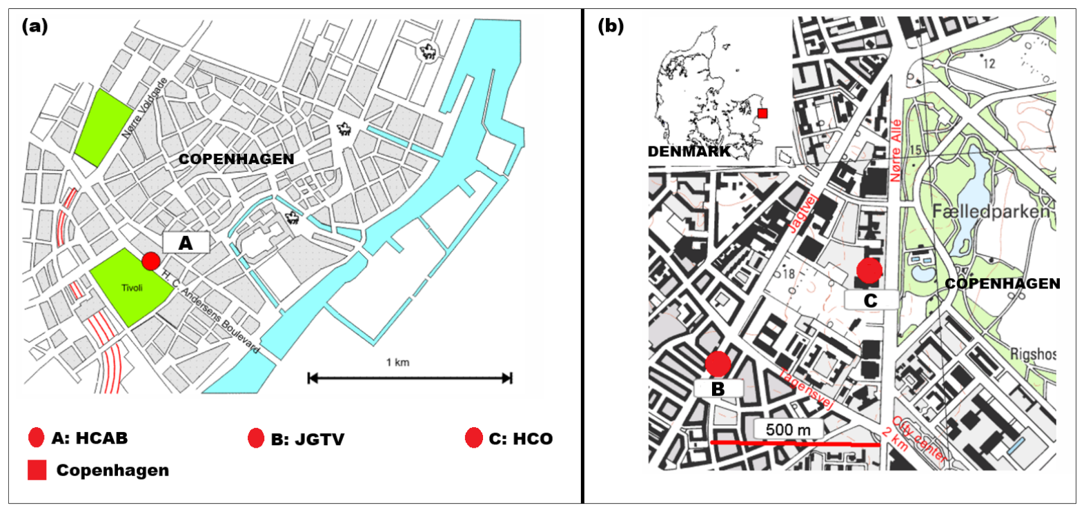
The study sites are two curbside air quality monitoring stations located in Copenhagen, Denmark: Hans Christian Andersens Boulevard (HCAB) and Jagtvej (JGTV) (Figure 1). Both stations are part of the Danish National Air Quality Monitoring Programme [39], managed by the Department of Environmental Science at Aarhus University, Roskilde [40]. They are equipped with high-quality EU reference-grade instruments that measure hourly concentrations of NO2, PM2.5, and other pollutants. In addition, a city-background monitoring station, Hans Christian Oersted (HCO), is situated near JGTV. Located on the rooftop of the University of Copenhagen’s HCO Institute, it provides hourly background measurements of NO2 and PM2.5 using the same high-grade equipment (Figure 1b). Quality assurance of the measured data is performed regularly to ensure consistency and reliability.
HCAB (Figure 1a) is one of the busiest streets in Denmark, with six lanes and continuous traffic flow averaging approximately 58,000 vehicles per day [41]. It is located opposite Tivoli, a popular amusement park that attracts significant tourist activity year-round. In contrast, JGTV (Figure 1b) is a two-lane street with relatively lower traffic volumes, averaging around 26,000 vehicles daily, and is flanked by buildings on both sides. The HCO station is situated on the rooftop of the University of Copenhagen, in a predominantly green and open area, with the busy road Norre Alle located approximately 35 m from the monitoring site (Figure 1b).
Figure 1.
Location of the study sites, Hans Christian Andersens Boulevard (HCAB) and Jagtvej (JGTV) street monitors, and the city-background monitor, Hans Christian Oersted (HCO) in Copenhagen, Denmark. (a) HCAB; (b) JGTV and HCO. Note: “Nørre Volgade” and “Nørre Allé” are the street names; “Fælledparken” is the name of a park in Copenhagen; blue colour = water; green = vegetation/greenery; black and grey = buildings and other land uses.
2.2. Data Curation
The data used in this study were obtained from the Danish National Air Quality Monitoring Programme [39], managed by the Department of Environmental Science at Aarhus University, Roskilde, Denmark. Quality-assured and quality-controlled measurements were provided by the measurement team at that institution.
Hourly NO2 concentrations were available for both HCAB and JGTV, covering the period from 2 March 2001 to 31 December 2018. Daily PM2.5 concentrations were available for HCAB only, spanning the period from 12 September 2012 to 31 December 2018. Background measurements of both pollutants were also collected from the HCO station for the same periods. All data were recorded in µg/m3. Details of the measurement methods are available on Aarhus University’s website [42]. Briefly, NO2 levels were measured using chemiluminescence, which detects light emitted during a chemical reaction with ozone. PM2.5 concentrations were determined using the Low Volume Sampling (LVS) gravimetric method, where particles are collected on filters and weighed in a laboratory to calculate daily averages.
It is important to note that a change in street layout occurred at the HCAB monitoring station in 2010, which brought traffic closer to the station [43]. Measurements from that year may be affected and should be interpreted with caution.
In addition to the air quality measurements, traffic and meteorological data were incorporated. The Department of Environmental Science at Aarhus University maintains a national GIS-based road network database [44], which includes information on vehicle counts, travel speeds, and street types for each road segment from 1960 to 2020. Street types are classified using the so-called OSPM road type, which links each segment to hourly traffic distributions by day and vehicle category (passenger cars, vans, small and large trucks, and buses). These distributions vary across weekdays, weekends, and the summer holiday month of July. This dataset was used to compile hourly traffic profiles, including vehicle counts, speeds, and composition, for the HCAB and JGTV study sites across the full measurement period.
Meteorological parameters are measured hourly at the HCO background monitoring station. Key variables include air temperature (°C), wind speed and direction (m/s and degrees), and relative humidity (%). These data were included in the model development and subsequent analysis for the same period. The daily variation in NO2, PM2.5, traffic, and meteorological variables for the 2017 validation year at HCAB and JGTV is shown in Appendix A (Figure A1, Figure A2 and Figure A3).
2.3. Data Preprocessing
All collected data were preprocessed using Python version 3.11. The analysis identified missing values in the NO2 and PM2.5 datasets, as well as in the traffic and meteorological data. Approximately 4% of the values were missing and were imputed using forward-fill, a method that preserves temporal consistency by relying solely on past observations. To maintain the integrity of the time series, no backward-filling or row deletion was performed.
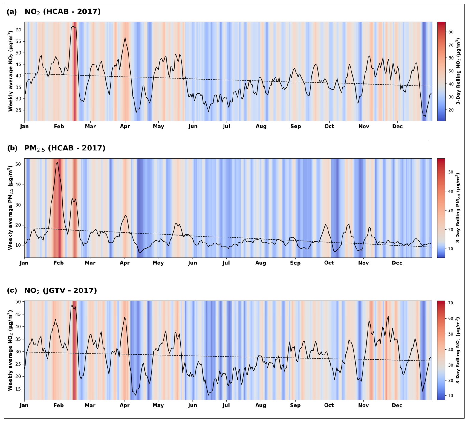
To visualise temporal trends in NO2 and PM2.5 concentrations, warming-stripes-style plots were generated for 2017 (Figure 2). Hourly NO2 data were aggregated into daily averages, while PM2.5 data were already available as daily means. A 3-day rolling mean was calculated for each pollutant and mapped to a sequential colour gradient from blue to red, representing low to high concentrations. These values are displayed as vertical colour stripes, one for each day of the year. A 7-day rolling mean was overlaid as a black line to highlight weekly trends, alongside a linear trend line indicating the overall direction of change. The left y-axis shows weekly mean concentrations (µg/m3), and a vertical colour bar on the right represents the corresponding 3-day rolling values.
The plots illustrate daily and seasonal variations in NO2 and PM2.5 concentrations at HCAB (Figure 2a,b) and NO2 at JGTV (Figure 2c). At HCAB, NO2 concentrations were generally higher during colder months, with peaks in late winter and late autumn and a declining trend through summer (Figure 2a). PM2.5 levels showed distinct episodic peaks in winter and early spring, followed by lower concentrations during warmer months (Figure 2b). At JGTV, NO2 levels were consistently lower than at HCAB but followed a similar seasonal pattern, with elevated concentrations in winter and autumn and a minimum in mid-summer (Figure 2c).
Figure 2.
(a) Daily variation in NO2 concentrations at the HCAB street location in 2017. The coloured stripes represent 3-day rolling mean NO2 concentrations (µg/m3), with red indicating higher and blue lower pollution levels. The black line shows the 7-day rolling average, and the dashed line indicates the linear trend over the year. (b,c) The same concentration levels for PM2.5 (HCAB) and NO2 (JGTV).
To characterise pollutant levels and assess variability across sites, basic descriptive statistics were computed in Python for the full dataset (Table 1). The count, mean, standard deviation, minimum, maximum, and quartile values were calculated for each variable, along with the percentage of missing values. These measures were derived separately for each monitoring site and pollutant type. The results show a wide range in pollutant concentrations, with HCAB street levels generally higher than JGTV and HCO. NO2 ranged from 0 to 283 µg/m3 at HCAB, with a mean of 51.9 µg/m3, while PM2.5 ranged from 3.6 to 83.3 µg/m3, averaging 16.5 µg/m3. Background site concentrations at HCO were considerably lower, with mean NO2 and PM2.5 levels approximately one-third lower than at HCAB, reflecting the influence of local traffic emissions (Table 1).
Table 1.
Summary statistics of NO2 and PM2.5 concentrations at the HCAB street site, JGTV street site, and HCO background site. Note: Std Dev = standard deviation, Min = minimum, Q1 = 25th percentile, Med = medium, Q3 = 75th percentile, Max = maximum.
The preprocessed data were then allocated for machine learning model development. For NO2, hourly measurements from HCAB and JGTV between 2 March 2001 and 31 December 2017 were used for training and testing. The complete hourly dataset from 2018 served as the independent holdout set for evaluation. For PM2.5 at HCAB, daily measurements from 12 September 2012 to 31 December 2017 were used for training and testing, while daily data from 2018 were reserved for independent evaluation. This chronological split was applied consistently across all modelling approaches.
Since the 2018 data were reserved as unseen for evaluation, the terms prediction and forecasting are used interchangeably throughout this study to refer to model outputs on previously unobserved data.
2.4. Machine Learning Models
A harmonised approach was adopted for data ingestion and feature engineering across all models and sites. A unified datetime index was built from the year, month, day, and hour for hourly series, and data were sorted chronologically. Calendar features were derived from the timestamp, including hour of day for hourly series, day of week, month, and a four-season code. Simple context flags were added, including weekend and public holiday indicators for key Danish holidays. For both sites, a rush-hour indicator was created covering the morning peak (07:00 to 09:00) and the afternoon peak (15:00 to 17:00). Cyclic patterns were captured by encoding periodic variables with sine and cosine transforms applied to hour and day of week for hourly data, and to day of week and month for daily data.
Outliers in the target series were identified using an Isolation Forest procedure applied to standardised values and were set to missing prior to imputation [45,46]. Isolation Forest is an unsupervised anomaly detection method that isolates observations by randomly selecting features and split values. It is based on the principle that anomalies require fewer partitions to separate from the rest of the data. This approach does not rely on distributional assumptions and performs well on high-dimensional environmental time series such as those used here.
After outlier removal, temporal features were engineered to capture both short- and long-term dependencies in pollutant concentrations. For each target variable, lagged predictors were created representing the most recent value, one hour prior for NO2 and one day prior for PM2.5, as well as a longer-term lag of 24 h for NO2 and seven days for PM2.5. Additional features described recent variability through rolling means and standard deviations, as well as first-order and seasonal differences. All temporal predictors were constructed exclusively from historical values to prevent data leakage.
An ablation study was conducted to assess the contribution of the short-term persistence feature. Persistence here refers to the tendency of pollutant concentrations to change gradually, making the most recent observed value a strong predictor of the next time step. The ablation involved removing the immediate lag feature, retraining the model, and comparing performance against the full-feature configuration. Removing the lag-1 predictor consistently degraded performance across all pollutant-site combinations, confirming that short-term persistence carries meaningful predictive information at the street level. This finding is consistent with the well-established role of pollutant autocorrelation in urban air quality modelling [12,25]. All final models reported in this study retain the lag-1 feature.
Following feature construction, the dataset was split chronologically. The training subset included data up to the end of 2016, and the testing subset comprised data from 2017. Predictor and target variables were scaled to a 0 to 1 range using MinMax transformation [47], with scaling parameters fitted on the training set and applied without modification to the test set. All models were trained in Python version 3.11 using TensorFlow 2.15.0, Keras, PyTorch 2.2, and scikit-learn 1.2.2.
2.4.1. Extreme Gradient Boosting
Extreme Gradient Boosting (XGB) is an ensemble learning algorithm that builds a sequence of regression trees, each correcting the residual errors of all previous trees using gradient descent. It incorporates regularisation, column and row subsampling, and histogram-based tree construction to reduce overfitting and improve generalisation [16,17]. In this study, separate XGB models were trained for each pollutant-site combination, hourly NO2 at HCAB and JGTV, and daily PM2.5 at HCAB.
For each dataset, the model was trained on data from 2001 to 2016 for hourly NO2 and from 2012 to 2016 for daily PM2.5 and tested on 2017 data. Key hyperparameters, including tree depth, learning rate, and regularisation strength, were tuned using time-aware cross-validation with five expanding windows on the training set. For NO2 models, a weighting scheme was applied to assign slightly higher importance to the top 5% of observed concentrations to help the model learn high-pollution episodes. For PM2.5, a similar spike-weighting strategy was tested but excluded from the final model as it did not yield meaningful improvements. Final models were trained on the full training dataset using the optimal number of boosting rounds. A full summary of hyperparameter configurations is provided in Table 2.
Table 2.
Hyperparameter configuration of the XGBoost (XGB) and Random Forest (RF) models for hourly NO2 and daily PM2.5 predictions. All models include lag-1 concentration as an input feature. Hyperparameters were optimised using time-series cross-validation on the training period (≤2016). Note: “-” in the table below indicates parameter not used or default configuration applied; n_estimators: number of trees (RF) or boosting rounds (XGB); max_depth: maximum tree depth controlling model complexity; learning_rate: boosting shrinkage factor controlling step size; min_child_weight: minimum instance weight required in a child node (XGB regularization); min_samples_split: minimum samples required to split a node (RF); min_samples_leaf: minimum samples required at a terminal leaf; subsample: fraction of training samples used per boosting iteration; colsample_bytree: fraction of features sampled per tree (XGB); gamma: minimum loss reduction required to perform a split (XGB); reg_alpha: L1 regularization strength; reg_lambda: L2 regularization strength; max_features: proportion of predictors considered at each split (RF); max_samples: fraction of training samples used per tree (RF); ccp_alpha: cost-complexity pruning parameter (RF).
2.4.2. Random Forest
Random Forest (RF) is an ensemble learning algorithm that constructs multiple decision trees independently and, in parallel, averages their predictions at the output stage. Each tree is trained on a bootstrap sample of the data and considers only a random subset of input features at each split, reducing overfitting and improving generalisation [19,20]. Separate RF models were trained for hourly NO2 at HCAB and JGTV, and for daily PM2.5 at HCAB, using the same chronological split as for XGB.
Hyperparameter tuning was conducted using grid search across key parameters, including the number of trees, maximum tree depth, minimum samples required for splits and leaf nodes, and the proportions of features and samples used during training. Time-aware cross-validation with expanding windows was applied throughout. Spike-weighting was not applied in RF training as it did not improve cross-validation performance. Final models were trained on the full training dataset using the best configurations identified. A full summary of hyperparameter settings for both XGB and RF is provided in Table 2.
2.5. Data Assimilation
Data assimilation (DA) provides a principled framework for combining model predictions with observational data to produce improved concentration estimates. In this study, DA was applied as a post-processing correction to the ML model outputs rather than to a physics-based transport model. The ML predictions served as the background field, and the measured pollutant concentrations at each site served as the observations. Two DA methods were implemented: three-dimensional variational assimilation (3D-Var) and the Extended Kalman Filter (EKF). Both methods were calibrated exclusively on the training period and applied without modification to the 2017 validation year and the 2018 independent test year. This design ensures that no information from the evaluation periods is entered into the DA configuration.
The background error variance (Q) was estimated from the residuals between the ML predictions and the observations on the training data. The observation error variance (R) was estimated as an empirical proxy derived from the high-frequency variability in the observed concentrations on the training data, specifically the variance of the first difference of the observed series scaled by a factor of 0.5. This approach approximates the noise component of the measurements without requiring instrument-specific error characterisation. The scalar Kalman gain K was then computed using Equation (1).
K = Q/(Q + R)
K represents the weight assigned to the observational correction relative to the ML background. A value of K close to 1 indicates that the observations dominate the analysis, while a value close to 0 indicates that the ML background is retained largely unchanged.
2.5.1. Three-Dimensional Variational Assimilation
Three-dimensional variational assimilation is a variational DA method that produces an analysis field by minimising a cost function balancing the departure of the analysis from the background and from the observations, weighted by their respective error variances [28,29]. In its scalar, single-station form applied here, the cost function simplifies to a closed-form solution. The analysis concentration x_a at each time step is given by Equation (2).
where x_b is the ML model background prediction, y is the observed concentration, and K is the scalar Kalman gain defined above. The correction at each time step is proportional to the innovation (y − x_b), moving the prediction toward the observation by the fraction K. The error variances Q and R are fixed at values estimated from the training period and held constant throughout the evaluation [31,32]. This formulation shares its mathematical foundations with variational assimilation methods applied at the regional scale in chemical transport modelling [28,35], but it is adapted here to operate directly on ML output at individual street sites.
x_a = x_b + K (y − x_b)
This formulation is computationally lightweight and straightforward to implement at single monitoring stations where spatial propagation of the correction is not required. It shares its mathematical foundations with variational assimilation methods applied at the regional scale in chemical transport modelling [28,35], but it is adapted here to operate directly on ML output at individual street sites.
2.5.2. Extended Kalman Filter
The Extended Kalman Filter (EKF) is a sequential DA method that updates the model state at each time step using the current observation and a propagated estimate of the prediction uncertainty [30,31]. Unlike 3D-Var, which applies a fixed correction gain, the EKF evolves the error covariance dynamically over time. In the scalar, single-station formulation applied here, the EKF update Equations (3)–(6) are given below.
where P is the evolving background error variance, Q is the process noise variance, R is the observation error variance, x_b,k is the ML background prediction at time step k, y_k is the observation, x_a,k is the analysis, and K_k is the time-varying Kalman gain. The filter is initialised with P equal to Q at the start of each evaluation period, using the same Q and R values estimated from the training period as described above. Because the EKF updates its gain dynamically, it can adapt to periods of sustained model bias, potentially offering advantages over the fixed-gain 3D-Var approach [30,32].
P_k|k − 1 = P_k−1 + Q
K_k = P_k|k − 1/(P_k|k − 1 + R)
x_a,k = x_b,k + K_k (y_k − x_b,k)
P_k = (1 − K_k) P_k|k − 1
Both DA methods were applied independently to XGB and RF predictions for all three pollutant-site combinations, producing six DA-corrected time series in total.
2.6. Model Evaluation and Assessment
Model performance was assessed using four standard metrics computed separately for the training period, the 2017 validation year, and the 2018 independent test year. Root mean square error (RMSE) measures the average magnitude of prediction errors, with greater sensitivity to large deviations. Mean absolute error (MAE) provides a linear measure of average error magnitude. The coefficient of determination (R2) quantifies the proportion of variance in the observed concentrations explained by the model. Mean bias error (MBE) captures the systematic direction of model error, where positive values indicate overestimation and negative values indicate underestimation. Together, these metrics provide a comprehensive picture of model accuracy, explained variance, and bias.
To evaluate performance specifically during high-concentration episodes, a spike metric was also computed. Spike events were defined as observed concentrations at or above the 90th percentile of the training distribution for each pollutant-site combination: 88.5 µg/m3 for HCAB NO2, 75.8 µg/m3 for JGTV NO2, and 28.5 µg/m3 for HCAB PM2.5. For these subsets, RMSE and MAE were computed separately to assess whether the models maintained accuracy during the most demanding conditions. Spike performance is of particular relevance for public health applications, where underestimation of peak concentrations carries the greatest risk of exposure misclassification.
All metrics were computed in Python using the scikit-learn library and standard numerical routines. Results are reported for all six model configurations across all three evaluation periods and all three pollutant-site combinations, giving a complete picture of how each ML model and DA method performed relative to one another. A full summary of performance metrics is provided in Table 3, with visual comparisons in Figures 3 and 4. Scatter density plots comparing observed and modelled concentrations for the 2018 independent test year are shown in Figure 5 for XGB and in Appendix A (Figure A4) for RF. Equivalent scatter plots for the 2017 validation year are provided in Appendix A (Figure A5 and Figure A6). Case study time-series analyses for the selected episode are presented in Figures 6–8, with RF equivalents in Appendix A (Figure A7, Figure A8 and Figure A9). Full-year time series for both evaluation years are provided in Appendix A (Figure A10, Figure A11, Figure A12 and Figure A13).
3. Results and Discussion
This section presents and discusses the performance of XGB and RF baseline models and the two DA methods, 3D-Var and EKF, applied as post-processing corrections to their predictions. Results are reported across three evaluation periods: the training period up to the end of 2016, the 2017 validation year, and the 2018 independent test year. The focus throughout is on the 2018 test year, as this represents model performance on fully unseen data. Performance is assessed for three pollutant-site combinations: hourly NO2 at HCAB, daily PM2.5 at HCAB, and hourly NO2 at JGTV.
3.1. Baseline ML Performance
Both XGB and RF produced meaningful predictions of NO2 and PM2.5 across all three pollutant-site combinations, though performance varied with site, pollutant, and evaluation period. Figure 3 presents the top 10 feature importances for each model and pollutant-site combination, providing insight into the key drivers of model predictions. The top row (Figure 3a–c) shows XGB-based results, and the bottom row (Figure 3d–f) shows the corresponding RF-based results.
Figure 3.
Feature importance for the XGBoost (XGB, top row, panels (a–c)) and Random Forest (RF, bottom row, panels (d–f)) models across the three pollutant-site combinations. Importance values are normalised to sum to 100%, and the top 10 features are shown for each configuration. Columns correspond to HCAB NO2 hourly (a,d), HCAB PM2.5 daily (b,e), and JGTV NO2 hourly (c,f). Feature importance for XGB is based on gain, and for RF on mean decrease in impurity. Note that x-axis scales differ between columns.
Across all NO2 configurations, short-term persistence dominated model predictions. The lag-1 concentration feature accounted for 41 to 54% of total feature importance across both XGB and RF at both sites, confirming that the most recent observed concentration is the strongest predictor of the next time step. Traffic variables, particularly heavy trucks, buses, and cars, were the second most important group, collectively contributing 10 to 18% in XGB and 8 to 15% in RF. Meteorological variables, including wind speed, wind direction, and mixing height, contributed a further 5 to 10%, reflecting the role of atmospheric dispersion conditions in modulating street canyon concentrations. Calendar and temporal features, including rush-hour indicators, day-of-week encoding, and hour of day, were more prominent in XGB than RF, suggesting that XGB captures the regularity of traffic emission patterns more explicitly through its gain-based importance metric.
For daily PM2.5 at HCAB, the feature importance structure differed markedly from NO2. The background PM2.5 concentration measured at HCO dominated predictions, accounting for 32% in XGB and 56% in RF, confirming that regional background transport is the primary driver of street-level PM2.5 at this site. Lag-1 concentration was the second most important feature at 14 to 15%, followed by meteorological variables including mixing height, wind direction, and global radiation, reflecting the influence of regional atmospheric conditions on PM2.5 accumulation and dispersion.
For hourly NO2 at HCAB, XGB achieved an RMSE of 8.1 µg/m3 on the training data, 8.7 µg/m3 in 2017, and 9.5 µg/m3 in 2018, with corresponding R2 values of 0.90, 0.83, and 0.81. See Table 3. RF performed slightly worse across all periods, with a 2018 RMSE of 10.1 µg/m3 and R2 of 0.78 (Table 3). The modest increase in RMSE from training to test year is expected. Street-level NO2 is sensitive to year-to-year variability in meteorological conditions, particularly wind speed, wind direction, and boundary layer height, which modulate how traffic emissions disperse within the street canyon. When the test year presents conditions not well represented in training, prediction accuracy declines. JGTV NO2 followed a similar pattern but with somewhat lower RMSE values, with XGB achieving 7.4 µg/m3 and R2 of 0.88 in 2018, and RF at 7.9 µg/m3 and R2 of 0.85. The lower absolute errors at JGTV compared to HCAB are consistent with JGTV’s lower traffic volume and lower peak concentrations, which reduce the magnitude of the prediction challenge. Both models capture a substantial proportion of the temporal variance in hourly NO2 at street level, consistent with findings from comparable tree-based ML studies of urban NO2 [20,22,23].
For daily PM2.5 at HCAB, XGB achieved an RMSE of 3.7 µg/m3 and R2 of 0.79 in 2018, while RF reached an RMSE of 4.5 µg/m3 and R2 of 0.75 (Table 3). The lower R2 values for PM2.5 relative to NO2, despite a smaller absolute RMSE, reflect the narrower concentration range of daily PM2.5 at this site, where even modest absolute errors account for a larger share of the total variance. Daily PM2.5 is also shaped by regional transport and secondary aerosol formation in addition to local traffic emissions, introducing variability that the traffic and meteorology features used here do not fully capture [8,37].
A full summary of all performance metrics, including MAE, R2, and MBE across all periods and configurations, is provided in Table 3. Both models show a positive MBE in 2018 for all pollutant-site combinations, indicating a systematic tendency to overestimate concentrations. For HCAB NO2, MBE was 4.2 µg/m3 for XGB and 4.3 µg/m3 for RF. For HCAB PM2.5, MBE was 2.2 µg/m3 for XGB and 1.7 µg/m3 for RF. For JGTV NO2, MBE was 2.6 µg/m3 for XGB and 2.9 µg/m3 for RF. This positive bias likely reflects two factors. First, the models were trained on a long historical period during which mean concentrations were generally higher due to older and more polluting vehicle fleets. Applying those trained models to the more recent test year, where real-world concentrations may have declined due to fleet renewal and lower traffic emissions, produces a systematic overprediction. Second, episodic low-concentration periods driven by strong wind events or unusually clean air masses are difficult to predict from the feature set alone and may further inflate the mean prediction above the observed mean.
Table 3.
Performance metrics for all six model configurations across three evaluation periods and three pollutant–station combinations. Note: RMSE = root mean square error; MAE = mean absolute error; R2 = coefficient of determination; MBE = mean bias error; All values are in µg/m3 except R2 (dimensionless); Train = training period (2001–2016 for NO2; 2012–2016 for PM2.5); 2017 = validation year; 2018 = independent test year (unseen data); XGB = XGBoost baseline; XGB + 3D-Var = XGBoost corrected by 3D-Var; XGB + EKF = XGBoost corrected by Extended Kalman Filter; RF = Random Forest baseline; RF + 3D-Var = Random Forest corrected by 3D-Var; RF + EKF = Random Forest corrected by Extended Kalman Filter. Yellow highlight indicates the lowest RMSE per period within each station block.
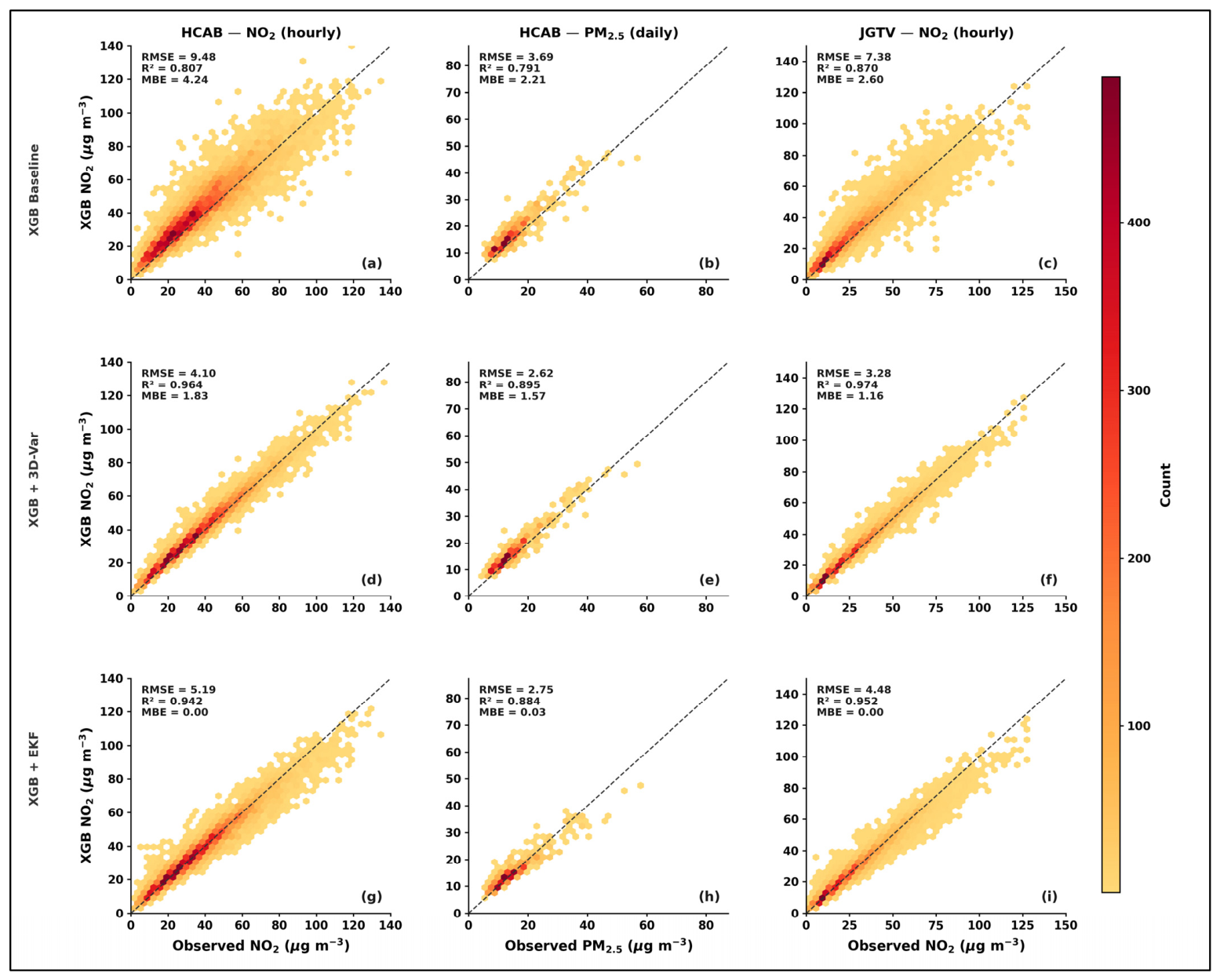
Scatter density plots for the 2018 test year confirm these patterns visually. See Figure 4. Panels (a), (b), and (c) show the XGB baseline predictions against observations for HCAB NO2, HCAB PM2.5, and JGTV NO2, respectively. The bulk of predicted concentrations align well with the 1:1 reference line at moderate concentrations, with greater scatter at the upper tail. This upper-tail scatter is characteristic of spike events, brief high-concentration episodes driven by combinations of heavy traffic, low wind speed, and unfavourable street canyon ventilation, which occur rarely, are underrepresented in training, and are not fully resolved by the traffic and calendar features alone. The RF equivalent scatter plots for 2018 are shown in Figure A4 in Appendix A. Scatter plots for the 2017 validation year are provided in Figure A5 and Figure A6 and show broadly consistent patterns across both years.
XGB consistently outperformed RF across all three pollutant-site combinations and all evaluation periods, though the margin was modest. The advantage was most apparent for HCAB PM2.5, where the 2018 RMSE difference was 0.8 µg/m3. For NO2 at both sites, differences were within 0.5 to 1.0 µg/m3. XGB’s sequential boosting approach, which iteratively corrects residual errors from previous trees, is particularly effective when the target variable exhibits complex non-linear interactions among predictors, as is the case for street-level NO2 driven by simultaneous variations in traffic volume, meteorology, and temporal patterns. RF, by contrast, builds trees independently and averages their outputs, which can be slightly less sensitive to these interactions but more robust in the presence of noisy predictors [22,23].
An ablation study confirmed that removing the lag-1 concentration feature consistently degraded prediction accuracy across all configurations, with RMSE increases ranging from approximately 10 to 25% depending on the pollutant and site. Street-level pollutant concentrations exhibit strong autocorrelation, particularly at hourly resolution, because the physical processes driving concentrations, traffic emissions, boundary layer mixing, and chemical transformation change gradually between consecutive time steps. The lag-1 feature encodes this persistence directly, providing the model with a highly informative starting point for each prediction [12,25]. All models presented here retain this feature.
Spike event performance for both baseline models is discussed in Section 3.4, with results shown in Figure 5. Full-year time series for both evaluation years are provided in Appendix A (Figure A10, Figure A11, Figure A12 and Figure A13) for both XGB and RF.
Figure 4.
Hexbin scatter density plots of observed versus modelled concentrations for the 2018 independent test year using XGBoost-based model (best performing ML model) configurations. Each hexbin cell is coloured by the number of data points it contains, as indicated by the shared colour bar. Rows correspond to the XGB baseline model (a–c), XGB combined with 3D-Var data assimilation (d–f), and XGB combined with the Extended Kalman Filter (g–i). Columns correspond to HCAB NO2 hourly concentrations (N = 8766), HCAB PM2.5 daily concentrations (N = 363), and JGTV NO2 hourly concentrations (N = 8766). The dashed line indicates the 1:1 reference. Performance metrics (RMSE, R2, MBE) are annotated in each panel in µg m−3. Note that y-axis scales differ between columns, reflecting the different concentration ranges of each pollutant.
3.2. Impact of 3D-Var Assimilation
Applying 3D-Var as a post-processing correction to both XGB and RF predictions produced consistent and substantial improvements across all three pollutant-site combinations and both test years. The correction operates by nudging each ML prediction toward the observed concentration at each time step, using a fixed scalar Kalman gain K estimated from the training period residuals. The Q, R, and K values for each configuration are provided in Table 4. For all pollutant-site combinations, K values ranged between 0.39 and 0.47, meaning that the 3D-Var correction assigned approximately 40 to 47% of the weight to the observational correction and retained the remaining 50 to 60% from the ML background. This reflects the fact that the ML predictions already carry substantial information about the observed concentrations, and the DA correction acts as a targeted refinement rather than a wholesale replacement of the background field.
Table 4.
Data assimilation configuration parameters estimated from the training period (≤2016) for each pollutant–station combination and ML model. Q denotes the process error variance derived from ML model residuals on training data. R denotes the observation error variance estimated as an empirical high-frequency proxy from the training observations. K is the scalar Kalman gain computed as K = Q/(Q + R), representing the weight assigned to the observational correction relative to the ML background. The observation weight (Obs weight) expresses K as a percentage. Note that K and Q/R values differ between XGB and RF for the same pollutant–station combination, reflecting differences in background error structure between the two ML models. The same K value applies to both 3D-Var and EKF configurations, as both use the same scalar gain formulation. Q = process error variance (from ML residuals on training data). R = observation error variance (empirical proxy). K = scalar Kalman gain = Q/(Q + R). Obs weight = K × 100 (%).
For hourly NO2 at HCAB, XGB + 3D-Var reduced the 2018 RMSE from 9.5 to 4.1 µg/m3, a reduction of 57%, while R2 improved from 0.81 to 0.96 (Table 3). MBE narrowed from 4.2 to 1.8 µg/m3, confirming that 3D-Var corrects a substantial portion of the systematic overestimation present in the baseline. The equivalent RF + 3D-Var configuration achieved an RMSE of 4.0 µg/m3 and R2 of 0.96 in 2018, with MBE falling to 1.7 µg/m3 (Table 3). Notably, RF + 3D-Var slightly outperformed XGB + 3D-Var in 2018 despite RF having the weaker baseline. This is because the 3D-Var correction is proportional to the innovation, the difference between the observation and the ML background, meaning that a model with larger baseline errors receives a larger correction at each step. The DA effectively compensates for the initial differences in ML baseline quality. Similar improvements were observed in 2017, with RMSE reductions of approximately 57% for XGB and 60% for RF relative to their respective baselines.
At JGTV, 3D-Var reduced the XGB baseline RMSE from 7.4 to 3.3 µg/m3 in 2018, while RF + 3D-Var achieved 3.6 µg/m3 (Table 3). R2 values reached 0.97 for both XGB and RF, indicating that the corrected models explain close to 97% of the temporal variance in hourly NO2 at this site. MBE values fell to 1.2 and 1.3 µg/m3 for XGB and RF, respectively, reflecting a near-elimination of systematic bias.
For daily PM2.5 at HCAB, XGB + 3D-Var reduced the 2018 RMSE from 3.7 to 2.6 µg/m3 and improved R2 from 0.79 to 0.89 (Table 3). RF + 3D-Var achieved an RMSE of 2.7 µg/m3 and R2 of 0.91, again slightly outperforming XGB after DA correction. The smaller relative improvement for PM2.5 compared to NO2, approximately 30% versus 57% RMSE reduction, is consistent with its smoother temporal structure and lower baseline error, which leaves less innovation for the DA correction to act on. When the ML background is already close to the observations, the Kalman gain provides only a modest correction, and the remaining error reflects variability that neither the ML nor the DA can resolve from the available features.
The scatter density plots for XGB + 3D-Var (Figure 4d–f) show markedly tighter clustering around the 1:1 reference line compared to the baseline panels above them, particularly in the mid to upper concentration range. The improvement is visible across all three pollutant-site combinations and is most pronounced for NO2, where the reduction in scatter at high concentrations indicates that 3D-Var is correcting precisely the episodes where the baseline model struggles most. RF + 3D-Var panels are shown in Figure A4d–f and display comparable patterns.
These results demonstrate that 3D-Var, even in its scalar single-station formulation, delivers meaningful and consistent improvement over standalone ML predictions at street level. The approach is computationally lightweight, requires no spatial covariance structure, and is fully calibrated from the training data without requiring any additional observations beyond those already available at the monitoring station. This makes it an operationally practical correction method for urban air quality monitoring networks where long-term ground measurements are available [28,29,32].
3.3. Impact of EKF Assimilation
The EKF produced improvements over the ML baseline across all configurations, but its gains were consistently smaller than those achieved by 3D-Var. Unlike 3D-Var, which applies a fixed correction gain throughout the evaluation period, the EKF updates its gain dynamically at each time step based on the evolving error covariance. The Q, R, and initial K values are the same as those used in the 3D-Var configurations (Table 4), but the EKF adjusts K over time as the predicted error covariance evolves through the forecast-update cycle.
For hourly NO2 at HCAB, XGB + EKF achieved a 2018 RMSE of 5.2 µg/m3 and R2 of 0.94, compared to 4.1 µg/m3 and 0.96 for XGB + 3D-Var (Table 3). RF + EKF reached 5.5 µg/m3 and R2 of 0.93 (Table 3). The improvement over the respective baselines was still substantial, approximately 45% RMSE reduction for both XGB and RF, but fell short of the 57% reduction achieved by 3D-Var. A notable feature of the EKF results is that MBE was reduced to approximately zero for all pollutant-site combinations, reflecting the filter’s sequential correction of systematic bias over time. For XGB + EKF, MBE was 0.0 µg/m3 at HCAB NO2 and JGTV NO2, and 0.0 µg/m3 at HCAB PM2.5. The same near-zero MBE pattern holds for RF + EKF. While 3D-Var also reduced MBE substantially, the EKF’s adaptive updating eliminates residual systematic bias more completely.
At JGTV NO2, XGB + EKF achieved an RMSE of 4.5 µg/m3 and R2 of 0.95 in 2018, while RF + EKF reached 4.6 µg/m3 and R2 of 0.95 (Table 3). These represent clear improvements over the baseline but sit notably above the 3.3 and 3.6 µg/m3 achieved by the corresponding 3D-Var configurations. For daily PM2.5 at HCAB, XGB + EKF reached an RMSE of 2.7 µg/m3 and R2 of 0.88, while RF + EKF achieved 3.6 µg/m3 and R2 of 0.84 (Table 3). The larger gap between 3D-Var and EKF for RF PM2.5 likely reflects the lower baseline RF accuracy for this pollutant, which provides a noisier background field that the EKF must correct with less stable gain dynamics.
The scatter density plots for XGB + EKF (Figure 4g–i) confirm these patterns. Clustering around the 1:1 line is tighter than the baseline but less compact than in the 3D-Var panels, particularly in the upper concentration range where the largest prediction errors tend to occur. RF + EKF scatter panels are shown in Figure A4g–i and display consistent patterns with slightly wider scatter than the RF + 3D-Var equivalents.
The consistent underperformance of EKF relative to 3D-Var in this study warrants discussion. The EKF’s dynamic gain adjustment offers the greatest benefit when model errors are non-stationary, that is, when prediction bias shifts substantially over time. In this study, the ML model errors appear relatively stationary across the evaluation periods, meaning the fixed-gain 3D-Var, calibrated on training residuals, already provides a near-optimal correction at each step. A second factor is the EKF’s spin-up behaviour. The filter initialises its error covariance at the start of each evaluation period and requires several time steps to converge toward a stable gain, during which the correction may be suboptimal. For the hourly NO2 series with 8766 observations per year, this spin-up period is negligible in proportion, but for daily PM2.5 with only 363 observations in 2018, the initialisation effect may be more consequential. These observations are consistent with findings from related DA literature, where fixed-gain methods have been shown to perform competitively when the underlying model error structure is stable [31,32].
Overall, both DA methods improve substantially on the ML baseline, with 3D-Var the preferred approach in terms of overall RMSE and R2 performance. The EKF remains a viable alternative, and its near-zero MBE makes it attractive in applications where eliminating systematic bias is a primary concern, for example, in long-term exposure assessments where cumulative overestimation could lead to health risk misclassification.
3.4. Spike Event Performance
Accurate prediction during high-concentration episodes is arguably the most policy-relevant challenge in street-level air quality modelling. Exceedances of regulatory thresholds are driven precisely by these spike events, and models that perform well on average but fail during peak episodes are of limited value for health protection and early warning. Figure 5 presents spike RMSE and MAE for all six model configurations across both evaluation years, with XGB-based results in the top row (Figure 5a–c) and RF-based results in the bottom row (Figure 5d–f). Solid bars show spike RMSE, and hatched bars show spike MAE. Results are shown for the 2017 validation year and the 2018 independent test year. Spike thresholds were defined as the 90th percentile of the training distribution for each pollutant-site combination, 88.5 µg/m3 for HCAB NO2, 75.8 µg/m3 for JGTV NO2, and 28.5 µg/m3 for HCAB PM2.5.
Both baseline ML models showed elevated errors during spike events relative to their overall performance. For HCAB NO2 in 2018, XGB baseline spike RMSE reached 12.5 µg/m3 and spike MAE reached 9.7 µg/m3 (Figure 5a, Table 3), substantially higher than the overall 2018 RMSE of 9.5 µg/m3. RF baseline spike RMSE was 13.4 µg/m3, and spike MAE was 10.4 µg/m3 (Figure 5d, Table 3), again exceeding its overall 2018 RMSE of 10.1 µg/m3. This pattern is consistent across all three pollutant-site combinations and both evaluation years, confirming that spike events represent a systematically harder prediction challenge for both ML models. High concentrations generally occur under specific combinations of heavy traffic load, low wind speed, and stable atmospheric conditions that are relatively rare in the training data and are not fully captured by the available feature set. This underrepresentation in training leads the models to regress toward mean concentrations during extreme episodes, producing larger errors precisely when accurate prediction matters most [22,37].
Figure 5.
Spike performance comparison across all model configurations for the three pollutant–station combinations. Spikes are defined as observed concentrations at or above the 90th percentile of the training period distribution, representing the upper tail of pollution events most relevant to air quality threshold exceedances. The top row (a–c) shows results for XGBoost-based models and the bottom row (d–f) for Random Forest-based models. Within each panel, bars are grouped by evaluation period (2017: validation; 2018: independent test), with six bars per group representing spike RMSE (solid) and spike MAE (hatched) for the baseline ML model, ML combined with 3D-Var (ML + 3D-Var), and ML combined with the Extended Kalman Filter (ML + EKF). The dashed vertical line separates the two evaluation years. Columns correspond to HCAB NO2 (hourly; (a,d)), HCAB PM2.5 (daily; (b,e)), and JGTV NO2 (hourly; (c,f)). Note that y-axis scales differ between columns. Spike thresholds correspond to 88.5 µg m−3 for HCAB NO2, 28.5 µg m−3 for HCAB PM2.5, and 75.8 µg m−3 for JGTV NO2.
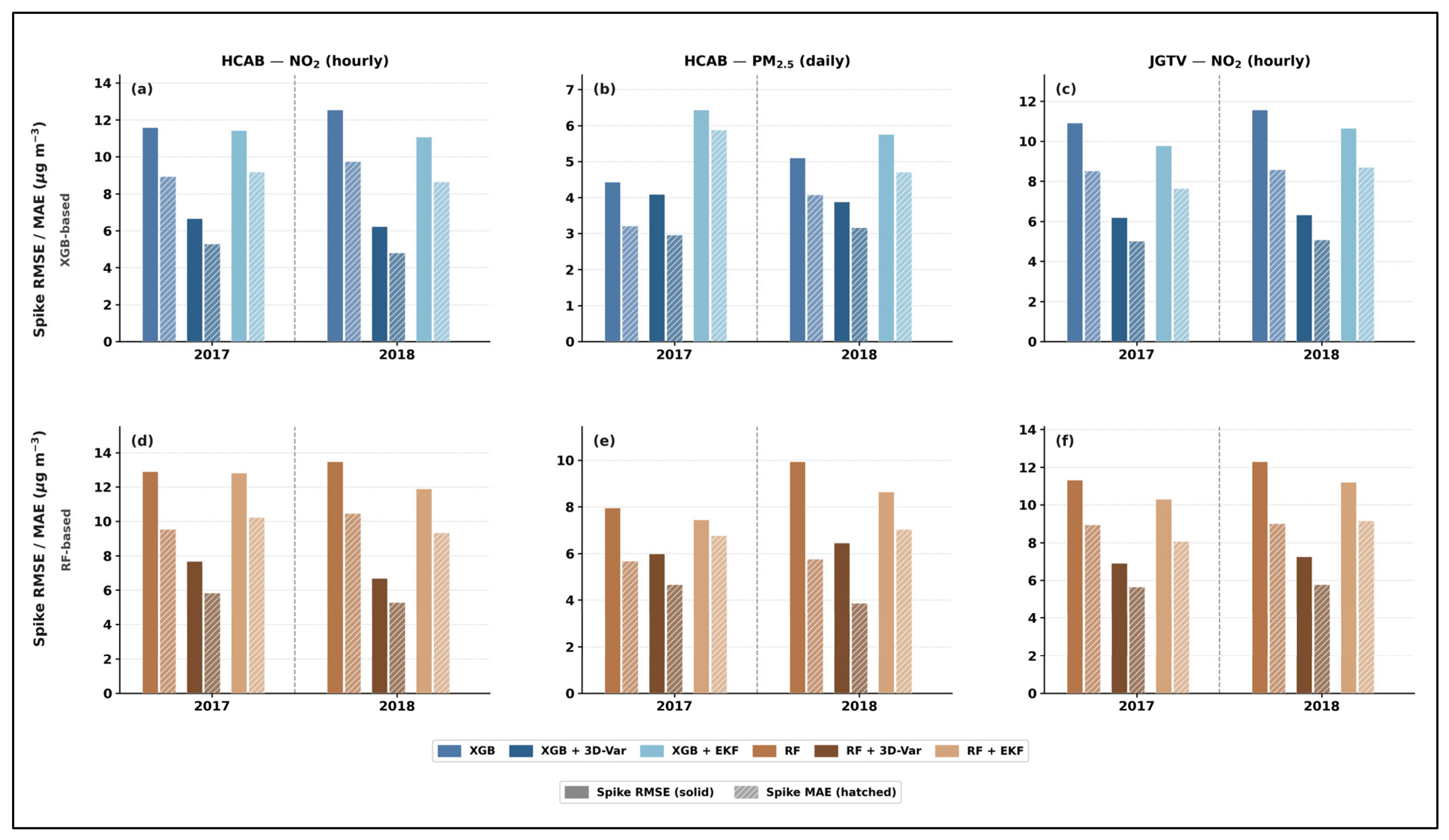
Both DA methods reduced spike errors substantially relative to their respective ML baselines. For HCAB NO2 in 2018, XGB + 3D-Var reduced spike RMSE from 12.5 to 6.1 µg/m3, a reduction of 51%, while XGB + EKF reduced it to 10.8 µg/m3, a reduction of 14% (Figure 5a). The pattern is similar for RF, where RF + 3D-Var reduced spike RMSE from 13.4 to 6.7 µg/m3 and RF + EKF reduced it to 11.9 µg/m3 (Figure 5d). These results confirm that 3D-Var is considerably more effective than EKF at reducing errors during spike events. This difference arises from the nature of spike episodes. During a spike, the observed concentration rises sharply above the ML background prediction, producing a large innovation. The fixed-gain 3D-Var immediately applies a proportional correction at each step, tracking the observed concentration closely throughout the episode. The EKF, by contrast, must propagate its error covariance through the spike, and its gain may not respond quickly enough to the sudden shift in prediction error, particularly at the onset of the episode.
At JGTV NO2, XGB + 3D-Var reduced spike RMSE from 11.5 to 6.3 µg/m3 in 2018, while XGB + EKF reached 10.6 µg/m3 (Figure 5c). RF + 3D-Var achieved 7.4 µg/m3 and RF + EKF 11.1 µg/m3 (Figure 5f). The relative advantage of 3D-Var over EKF is largest at JGTV, likely because JGTV has lower baseline traffic volume and fewer sustained spike episodes, meaning that when spikes do occur, they tend to be more episodic and short-lived, favouring the fixed-gain correction approach.
For daily PM2.5 at HCAB, both DA methods produced more modest spike error reductions. XGB + 3D-Var reduced spike RMSE from 5.1 to 3.8 µg/m3 in 2018, while XGB + EKF achieved 5.6 µg/m3, slightly worse than the baseline (Figure 5b). RF + 3D-Var reduced spike RMSE from 10.0 to 6.5 µg/m3, while RF + EKF reached 7.0 µg/m3 (Figure 5e). The EKF’s inability to improve on the XGB baseline for PM2.5 spike events reflects the daily temporal resolution of this series. With only one observation per day, the EKF has fewer opportunities to update its gain and track episodic behaviour. The 3D-Var, operating with a fixed gain calibrated on training residuals, is more stable under these conditions.
Across all configurations and pollutant-site combinations, 3D-Var consistently achieved the lowest spike RMSE and MAE, making it the preferred method for applications where peak episode accuracy is the primary concern. The case study analysis in Section 3.5 examines a specific high-error episode in detail, illustrating how the two DA methods behave differently during a sustained spike period.
3.5. Case Study: May 2018 Episode
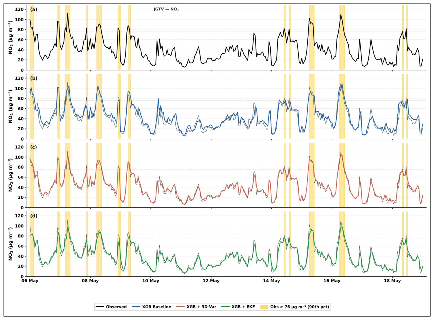
To examine model behaviour during a sustained high-error period, a two-week case study was conducted for the episode from 6 to 19 May 2018. This window was selected as the 14-day period in 2018 with the highest XGB baseline RMSE for HCAB NO2, where the episode RMSE reached 14.0 µg/m3 compared to the full-year baseline of 9.5 µg/m3. The selected episode, therefore, represents the most challenging prediction period in the independent test year. The same window is used for all three pollutant-site combinations to allow direct comparison across sites and pollutants. Figure 6, Figure 7 and Figure 8 show the observed and modelled time series for HCAB NO2, HCAB PM2.5, and JGTV NO2, respectively, for XGB-based configurations. The equivalent RF-based figures are provided in Appendix A (Figure A7, Figure A8 and Figure A9).
At HCAB NO2, the episode is characterised by repeated short-duration spikes above the 90th percentile threshold of 88.5 µg/m3, concentrated in the first half of the episode (6 to 9 May) and again around 14 to 17 May (Figure 6). The XGB baseline captures the general diurnal structure and the broad seasonal level reasonably well, but it consistently underestimates the magnitude of individual spikes and smooths out the sharp peaks that characterise the highest-concentration hours. This behaviour is typical of tree-based ML models trained on long historical records, where rare high-concentration events are diluted by the much larger volume of moderate-concentration observations, causing the model to learn a prediction that is biased toward typical rather than extreme conditions.
XGB + 3D-Var tracks the observed concentrations substantially more closely throughout the episode (Figure 6c). The innovation, the difference between the observation and the ML background, is large during spike hours, and the fixed-gain correction pulls the analysis toward the observed value at each step. The result is a time series that follows both the rising and falling edges of individual spikes with considerably greater fidelity than the baseline. XGB + EKF also improves on the baseline but responds more slowly to the onset of spike events and shows a tendency to lag behind the observed concentrations during the most rapid rises (Figure 6d). This lag reflects the EKF’s sequential error covariance propagation, which requires several time steps to fully adjust its gain following a sudden change in prediction error. The thin dark grey reference line in panels (b), (c), and (d) reproduces the observed record, making the departure of each model from the observations directly visible.
Figure 6.
Time series of observed and modelled hourly NO2 concentrations at the HCAB street site during the selected case study episode (6–19 May 2018), corresponding to the 14-day window with the highest XGBoost baseline RMSE in the 2018 independent test year. Panel (a) shows the observed concentrations. Panels (b), (c), and (d) show the XGB baseline, XGB + 3D-Var, and XGB + EKF model outputs, respectively; the thin dark grey line in each panel reproduces the observed record for visual reference. Amber shading indicates hours where observed NO2 exceeded the 90th percentile training threshold (88.5 µg m−3). The horizontal dotted line marks this spike threshold.
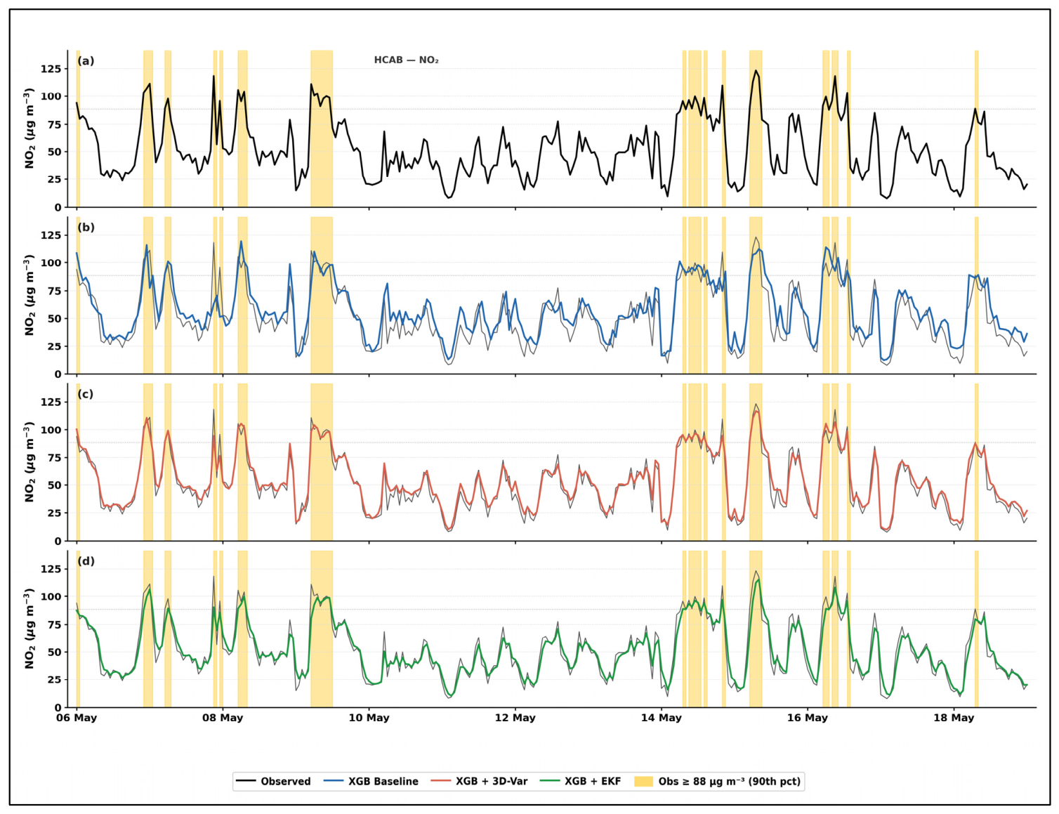
At HCAB PM2.5, the episode shows a more gradual concentration pattern consistent with daily averaging (Figure 7). No observations exceed the 28.5 µg/m3 spike threshold during this window, confirming that the selected episode is primarily a NO2 episode driven by traffic and street canyon ventilation conditions rather than a PM2.5 event. The XGB baseline overestimates PM2.5 concentrations throughout the episode, consistent with the positive MBE reported in Section 3.1. XGB + 3D-Var and XGB + EKF both reduce this overestimation and track the observed daily cycle more closely, with 3D-Var achieving tighter agreement, particularly during the modest concentration rise in the second half of the episode.
At JGTV NO2, the episode pattern broadly mirrors HCAB but with lower absolute concentrations and somewhat fewer spike exceedances above the 75.8 µg/m3 threshold (Figure 8). The XGB baseline again underestimates peak concentrations, and both DA methods improve on this. XGB + 3D-Var achieves notably lower errors during the spike periods around 7 to 9 May and 14 to 16 May, while XGB + EKF shows similar lag behaviour as observed at HCAB.
Figure 7.
Time series of observed and modelled daily PM2.5 concentrations at the HCAB street site during the same case study episode (6–19 May 2018) as Figure 6. Panel (a) shows the observed concentrations. Panels (b), (c), and (d) show the XGB baseline, XGB + 3D-Var, and XGB + EKF model outputs, respectively; the thin dark grey line reproduces the observed record for reference. No observed PM2.5 concentrations exceeded the 90th percentile training threshold (28.5 µg m−3) during this episode, indicating that the selected window represents a NO2 pollution episode rather than a PM2.5 event.
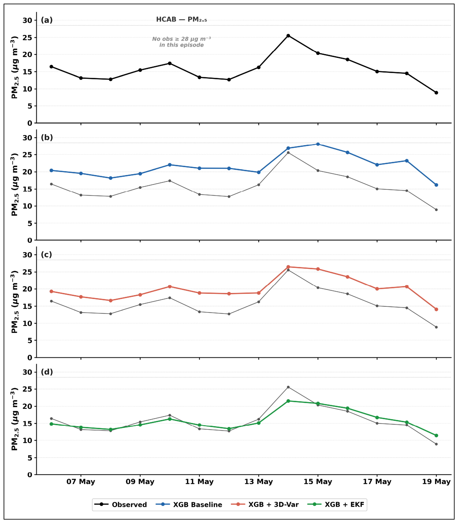
Figure 8.
Time series of observed and modelled hourly NO2 concentrations at the JGTV street site during the same case study episode (6–19 May 2018) as Figure 6. Panel (a) shows the observed concentrations. Panels (b), (c), and (d) show the XGB baseline, XGB + 3D-Var, and XGB + EKF model outputs, respectively; the thin dark grey line reproduces the observed record for reference. Amber shading indicates hours where observed NO2 exceeded the 90th percentile training threshold (75.8 µg m−3).
The RF-based case study results for all three pollutant-site combinations are shown in Figure A7, Figure A8 and Figure A9. The RF baseline shows broadly similar behaviour to XGB, reasonable mean-level prediction with underestimation of peak concentrations, consistent with the slightly higher baseline RMSE reported in Section 3.1. RF + 3D-Var achieves comparable improvement to XGB + 3D-Var, while RF + EKF shows the same lag behaviour at spike onset. This consistency across both ML models reinforces the conclusion that the performance differences observed in this case study are driven by the DA method rather than the choice of ML background.
Taken together, the case study results illustrate the practical value of DA correction at the street level. During the most challenging prediction period of the independent test year, 3D-Var reduced episode RMSE by more than 50% relative to the ML baseline, transforming a model that frequently misses peak concentrations into one that tracks observed spikes with substantially greater accuracy. This level of improvement has direct relevance for air quality warning systems, where accurate prediction of high-concentration hours is critical for protecting public health.
3.6. Synthesis and Comparison with the Literature
The results of this study demonstrate that tree-based ML models can predict street-level NO2 and PM2.5 with meaningful accuracy across multi-year periods at Copenhagen traffic sites, and that both 3D-Var and EKF post-processing corrections deliver substantial and consistent improvements over the ML baseline. This section positions the findings in relation to the broader literature and highlights the unique contributions of the approach adopted in this study.
The baseline XGB and RF performance reported in this study compares favourably with published results from comparable settings. Zhang et al. [48] applied XGB, RF, and LSTM to improve 1-to-3-day deterministic air pollution forecasts at urban traffic and background sites in Stockholm, Sweden, the most geographically and climatically comparable published study to this work. Using a combination of meteorological forecasts and deterministic model output as predictors, their best configurations achieved RMSE reductions of 20 to 40% over raw deterministic forecasts for NO2 at traffic sites. Our XGB baseline RMSE values of 9.5 µg/m3 for HCAB NO2 and 7.4 µg/m3 for JGTV NO2 in 2018 are broadly consistent with this range, noting that our models predict directly from measured concentrations and traffic data rather than from deterministic model output, making the tasks not directly equivalent. Zaman et al. [13], using RF for PM2.5 prediction across Malaysia with ground-based observations, reported R2 values in the range 0.70 to 0.85 depending on site and season, which aligns with our RF baseline R2 of 0.75 to 0.85 across pollutant-site combinations. Méndez et al. [25], in a comprehensive review of ML algorithms for air quality forecasting, identify XGB and RF as consistently among the top-performing methods for tabular, station-based prediction tasks, with the performance advantage of XGB over RF being modest but reproducible across diverse datasets, precisely the pattern we observe here.
The DA results are more novel and require more careful contextualisation, as comparable street-level applications are rare. The closest published analogue remains Lu et al. [32], who combined LSTM with 3D-Var for PM2.5 forecasting in China and demonstrated that the hybrid system substantially outperformed the standalone LSTM. They reported RMSE reductions of approximately 30 to 50% for PM2.5 after assimilation, broadly consistent with our 3D-Var PM2.5 improvements of approximately 30% for both XGB and RF. However, their system operated at the city scale with the ML model serving as a surrogate for a CTM, whereas our application corrects ML predictions directly at individual street monitoring stations, a methodologically distinct and computationally simpler approach. Huang et al. [33], combining a nudging DA scheme with an extremely randomised tree model applied to CTM emission adjustment in China, reported PM2.5 RMSE reductions from 24.4 to 10.0 µg/m3, a reduction of approximately 59% in a single episode. Our 3D-Var RMSE reductions of 57% for HCAB NO2 and 29% for HCAB PM2.5 in 2018 are of comparable magnitude for NO2, while the PM2.5 improvements are smaller because our baseline PM2.5 errors are already substantially lower in absolute terms.
Cai et al. [24] developed a hybrid ConvLSTM-EnKF system for spatiotemporal PM2.5 forecasting across China, demonstrating that periodically assimilating real-time observations into a data-driven model reduced accumulated forecast error significantly and enabled operational forecasts up to one month ahead with spatially averaged RMSE below 20 µg/m3. Their work demonstrates the growing interest in hybrid DA-ML architectures operating directly on data-driven models rather than CTMs, which is the same methodological territory this study occupies. The key difference is spatial scale: their system covers a large regional domain, while we operate at individual street stations. At the station scale, the simpler scalar 3D-Var formulation we apply is sufficient and avoids the computational overhead of ensemble-based methods.
The relative performance of 3D-Var versus EKF in this study adds to a small but growing body of comparative DA literature. Dash et al. [49] compared 3D-Var, EnKF (Ensemble Kalman Filter), and EnSRF (Ensemble Square Root Filter) for PM2.5 prediction in East Asia using the CMAQ model and found that ensemble-based methods generally outperformed 3D-Var, particularly for predictions extending beyond 24 h, where the fixed background error covariance of 3D-Var became a limiting factor.
Djalalova et al. [50] applied Kalman filtering combined with analogue forecasting as a post-processing correction to CMAQ PM2.5 forecasts across 570 monitoring sites in the contiguous United States, achieving MAE reductions of 44 to 52% and correlation improvements of 13 to 30% over the raw CMAQ output across a full year. Their study reinforces two findings directly relevant to ours: first, that Kalman filter-based post-processing consistently outperforms simple running-mean bias subtraction and delivers improvements that are robust across all seasons; second, that the magnitude of improvement is largest in winter when model bias is greatest, precisely the season in which our ML baseline errors are also highest at the Copenhagen street sites. While their approach applied KF to a CTM background rather than an ML background, the correction mechanism is mathematically equivalent to the scalar 3D-Var and EKF formulations used here, and the performance gains are of comparable magnitude to those we report for NO2 and PM2.5.
Wang et al. [51] provide a systematic overview of KF variants and their atmospheric data assimilation applications, emphasising that EKF is well suited to low-dimensional, single-station correction tasks where the error structure is approximately Gaussian, a setting directly analogous to ours. Our finding that EKF achieves near-zero MBE while 3D-Var retains small residual bias is consistent with the EKF’s recursive bias-tracking mechanism described in this literature [51]. The finding that 3D-Var outperforms EKF in overall RMSE at our sites is consistent with Dash et al.’s observation [49] that fixed-gain variational corrections are competitive or superior when the prediction error structure is stationary, while ensemble or adaptive methods offer greater benefit when errors evolve dynamically.
Tučkus et al. [34] demonstrated similar findings in the DyNA framework applied to Italian monitoring networks, where DA consistently reduced forecast errors across sites and pollutants, with the magnitude of improvement depending on baseline model performance and site-specific characteristics. Their work reinforces the general conclusion emerging from this study: DA post-processing is a robust and practically accessible way to improve station-based ML predictions, regardless of the specific ML model used as the background.
A key finding that is largely absent from the existing literature is the explicit evaluation of DA performance during spike events. Most published ML and DA studies report only full-period aggregate metrics, which can mask substantial underperformance during the high-concentration episodes that are most consequential for public health [22,25]. Our results show that 3D-Var reduces spike RMSE by up to 51% for HCAB NO2, while EKF achieves only 14% reduction, making the choice of DA method highly consequential for applications that prioritise episode accuracy. This finding has direct relevance for air quality warning systems and regulatory exceedance assessment, representing a methodological contribution that extends beyond the specific context of Copenhagen.
Geographically, Copenhagen’s street sites have received very limited attention in the ML modelling literature, despite the availability of one of the longest high-quality continuous measurement records in Northern Europe. The results presented here, covering 17 years of training data and two full independent evaluation years, demonstrate that tree-based ML models calibrated on long observational records can generalise well across annual cycles, seasonal transitions, and changing emission environments. This multi-year evaluation scope is substantially longer than the majority of published street-level ML studies, which typically assess model performance over single years or shorter periods [24,25,48]. The model results also reveal stable and reproducible temporal patterns across the full evaluation period. The consistent seasonal cycle, with higher NO2 and PM2.5 concentrations in cold months driven by reduced boundary layer mixing and stable atmospheric conditions, together with the diurnal and weekly concentration patterns captured by the rush-hour and day-of-week features, confirms that the key drivers of street-level pollution at these Copenhagen sites are well represented by the feature set and remain consistent across years.
4. Strengths and Limitations
This section discusses the main strengths of this study and acknowledges its limitations.
The most notable strength of this study is its multi-year evaluation scope. With training data spanning up to 17 years and two fully independent evaluation years, this is one of the longest temporal evaluations of ML-based street-level air quality prediction reported in the peer-reviewed literature. Most comparable studies assess model performance over single years or short episodes [24,25,48]. The extended scope allows the models to be tested across multiple seasonal cycles, varying meteorological regimes, and gradual changes in the emission environment, providing a more demanding and realistic assessment of generalisation ability than short-horizon evaluations.
A second strength is the systematic and consistent evaluation design. Two ML models, two DA methods, and three pollutant-site combinations were all evaluated under identical conditions across the same training, validation, and test periods. This parallel structure allows direct and fair comparison between XGB and RF, and between 3D-Var and EKF, without confounding differences in data preparation or evaluation period. The inclusion of explicit spike event metrics, which most published ML and DA studies omit, adds a further dimension of policy-relevant evaluation that is directly connected to regulatory threshold exceedances and public health protection [22,25].
A third strength is the computational simplicity of the framework. The DA correction requires only the ML model output and the observed concentration at the same station. No spatial covariance structure, ensemble, adjoint model, or emission inventory is needed. Q, R, and K are estimated entirely from training residuals, and the correction itself requires a single arithmetic operation per time step. This makes the framework straightforward to implement and maintain in an operational monitoring context, wherever long-term ground observations are available. It should be noted, however, that the simultaneous availability of quality-assured pollutant, meteorological, and traffic data used in this study reflects the well-established infrastructure of the Danish National Air Quality Monitoring Programme, which may not be universally available at all urban monitoring sites. Similarly, while the scalar DA formulation is mathematically simple, careful attention to error variance estimation and the stationarity assumption underlying the fixed-gain correction is required for reliable application in other settings.
This study also has important limitations that should be acknowledged. First, the analysis is limited to two street sites in a single Northern European city. While Copenhagen provides a well-monitored and representative urban traffic environment, the generalisability of the results to cities with different street canyon geometries, traffic compositions, climatic conditions, or emission profiles has not been tested. Results from cities with higher baseline concentrations, more complex topography, or stronger secondary aerosol formation may differ from those reported here.
Second, the DA parameters Q, R, and K are estimated from training period residuals and held fixed throughout the evaluation. This assumes that the error structure of the ML model is approximately stationary over time. In practice, substantial changes in traffic volume, fleet composition, or urban infrastructure, such as the 2010 street layout change at HCAB noted in Section 3.2, can alter the model error structure in ways that the fixed-gain correction cannot fully accommodate. A fully adaptive DA system that recalibrates its parameters continuously would be more robust to such non-stationarities, at the cost of added complexity.
Third, the DA correction at each station is applied independently, with no spatial propagation of the analysis increment to neighbouring locations. In a network of closely spaced monitoring stations, observations at one site carry information about nearby concentrations that is not exploited here. Spatial DA methods that propagate corrections across a network could potentially deliver additional improvements, particularly during episodes when a pollution plume affects multiple sites simultaneously.
Fourth, PM2.5 data were available only as daily averages at HCAB. This limits the temporal resolution of the PM2.5 analysis relative to the hourly NO2 analysis and means that the DA correction for PM2.5 operates on a much sparser observation sequence, 363 daily values in 2018 compared to 8766 hourly values for NO2. The lower number of DA update steps reduces the EKF’s ability to converge and adapt, which may partly explain its weaker performance relative to 3D-Var for PM2.5.
5. Conclusions
This study applied XGBoost and Random Forest to predict hourly NO2 and daily PM2.5 at two traffic-dominated street sites in Copenhagen, Denmark, across an evaluation period spanning two independent years. Both models produced meaningful predictions, with XGB achieving RMSE values of 9.5 µg/m3 for HCAB NO2 and 7.4 µg/m3 for JGTV NO2 in the 2018 independent test year, and R2 values of 0.81 and 0.88, respectively. RF performed slightly worse in all configurations. Both models showed a systematic positive bias and reduced accuracy during high-concentration spike events, reflecting the well-known difficulty of tree-based models in resolving rare extreme episodes from long historical training records. These results confirm that tree-based ML models can generalise well across multi-year periods at street level when trained on rich observational records combining traffic, meteorology, and temporal features.
Applying 3D-Var and EKF as post-processing corrections to both ML models produced consistent and substantial improvements across all pollutant-site combinations and both evaluation years. Three-dimensional variational assimilation reduced RMSE by approximately 57% for hourly NO2 and 30% for daily PM2.5 relative to the XGB baseline in 2018, while EKF achieved reductions of approximately 45% for NO2 with near-complete elimination of systematic bias. For spike events, 3D-Var reduced spike RMSE by up to 51% for HCAB NO2, while EKF achieved only 14%, a finding with direct relevance for air quality warning systems and regulatory exceedance assessment. Overall, 3D-Var is the preferred method where overall accuracy and spike performance are the primary concern, while EKF is the preferred choice where eliminating systematic bias is the priority, for example, in long-term exposure assessment.
The DA correction framework developed here is computationally lightweight, requires no spatial covariance structure or ensemble, and is fully calibrated from residuals in the training period. It is agnostic to the choice of background model. The same correction can, in principle, be applied to any deterministic prediction at a monitoring station, whether from a tree-based machine-learning model, a neural network, or a physics- and chemistry-based dispersion model such as OSPM, ADMS-Urban, or AERMOD. As such, the framework is not intended to replace existing dispersion modelling approaches but to serve as a practical complement, reducing the systematic biases and random errors that persist in deterministic street-level air quality predictions. This provides a practical route to improved operational forecasting at street level wherever long-term ground observations are available, directly supporting urban air quality agencies, public health authorities, and city planners in obtaining timely concentration estimates for exposure assessment, compliance monitoring, and targeted emission reduction planning.
6. Outlook and Future Work
Future work should focus on three directions. First, the framework should be tested at additional urban sites and cities with different street canyon geometries, traffic compositions, and meteorological conditions to assess its generalisability beyond the Copenhagen context. Second, the approach should be extended to physics- and chemistry-based dispersion models such as OSPM, AERMOD, and ADMS-Urban as the background field, allowing DA post-processing to correct systematic biases in deterministic street and city-scale air quality predictions. Third, testing the framework in a true operational forecasting setting, with rolling DA parameter recalibration and real-time correction on consecutive forecast horizons, would establish its practical readiness for integration into urban air quality monitoring and early warning systems. Fourth, while this study deliberately focused on tree-based ML models as robust and interpretable baselines, future work could explore neural network architectures as background fields for the DA correction, building on the extensive existing literature on deep learning for air quality forecasting [48]. Finally, future work should focus on translating improved spike event prediction into actionable warning frameworks and policy response protocols, bridging the gap between forecasting and practical urban environmental management.
Author Contributions
Conceptualization, methodology, data curation, quality assurance, software, validation, formal analysis, investigation, visualization, resources, supervision, writing—original draft preparation, writing—review and editing, J.K.; data curation and quality assurance, writing—review and editing, R.K. and C.N. All project supervision and administration were carried out by J.K. All authors have read and agreed to the published version of the manuscript.
Funding
This research received no external funding.
Institutional Review Board Statement
Not applicable.
Informed Consent Statement
Not applicable.
Data Availability Statement
The data generated and the code developed during this study that support the reported results and analysis are not publicly archived but are available upon reasonable request. Researchers interested in accessing the dataset or the code used for model development and data assimilation are encouraged to contact the corresponding author directly by email.
Acknowledgments
During the preparation of this manuscript, the authors used the following tools for the purposes described. Web of Science, Scopus, and Google Scholar were used for systematic literature search and screening. Scite AI (https://scite.ai, institutional subscription) (accessed on 4 February 2026) and Perplexity AI (https://www.perplexity.ai, free tier) (accessed on 4 February 2026) were used to assist with literature discovery, research gap identification, and synthesis of relevant studies. Microsoft Copilot (standard institutional subscription) (accessed on 4 March 2026) was used for text rephrasing and restructuring of selected passages. The authors have reviewed and edited all outputs from these tools and take full responsibility for the content of this publication.
Conflicts of Interest
The authors declare no conflicts of interest.
Abbreviations
The following abbreviations are used in this manuscript:
| AQD | Air Quality Directive |
| CTM | Chemical Transport Model |
| DA | Data Assimilation |
| EC | European Commission |
| EEA | European Environment Agency |
| EKF | Extended Kalman Filter |
| EU | European Union |
| GIS | Geographic Information System |
| HCAB | Hans Christian Andersens Boulevard |
| HCO | Hans Christian Oersted |
| JGTV | Jagtvej |
| LVS | Low Volume Sampling |
| MAE | Mean Absolute Error |
| MBE | Mean Bias Error |
| MinMax | Min-Max Normalisation |
| ML | Machine Learning |
| NO2 | Nitrogen Dioxide |
| PM | Particulate Matter |
| PM2.5 | Particulate Matter with aerodynamic diameter less than 2.5 µm |
| R2 | Coefficient of Determination |
| RF | Random Forest |
| RMSE | Root Mean Square Error |
| WHO | World Health Organization |
| XGB | Extreme Gradient Boosting |
| 3D-Var | Three-Dimensional Variational Assimilation |
Appendix A
This appendix provides supplementary figures supporting the data description, model development, and results presented in the main text. Figure A1, Figure A2 and Figure A3 show the daily variation in pollutant concentrations alongside traffic and meteorological variables for the 2017 validation year at the HCAB and JGTV monitoring sites, supporting Section 3.2. Figure A4, Figure A5 and Figure A6 present scatter density plots for RF-based model configurations in 2018 and XGB and RF configurations in 2017, complementing Figure 4 in Section 3.1. Figure A7, Figure A8 and Figure A9 present case study time series for RF-based model configurations during the May 2018 episode, equivalent to Figure 6, Figure 7 and Figure 8 in Section 3.5. Figure A10, Figure A11, Figure A12 and Figure A13 present full-year time series for XGB and RF across the 2017 validation year and 2018 independent test year, supporting Section 3.1, Section 3.2, Section 3.3, Section 3.4 and Section 3.5.
Figure A1 shows NO2, traffic, and meteorological conditions at HCAB for 2017. Street and background NO2 concentrations follow a clear seasonal cycle, with higher values in winter and lower values during summer. Vehicle counts remain relatively stable throughout the year, while wind speed, temperature, and humidity show the expected seasonal patterns for a Northern European urban environment.
Figure A2 shows the equivalent data for PM2.5 at HCAB. The PM2.5 series is characterised by episodic peaks in late winter and early spring, followed by a sustained period of lower concentrations through summer and a modest increase in autumn. Background PM2.5 follows a broadly similar pattern, though peak values are lower, consistent with the role of local traffic in elevating street-level concentrations.
Figure A3 shows NO2, traffic, and meteorological data for 2017 at JGTV. Concentrations at this site are lower than at HCAB, reflecting the lower traffic volume, but the seasonal pattern is broadly similar. Wind conditions and temperature follow the same annual cycle as observed at HCAB, consistent with the proximity of the two sites within the same city.
Figure A1.
Daily NO2, traffic, and meteorological variables for 2017 at HCAB. Panels show street NO2 (µg/m3), background NO2 (µg/m3), daily vehicle counts (vehicles/day), wind speed (m/s), wind direction (degrees), temperature (°C), and relative humidity (%), from January to December 2017.
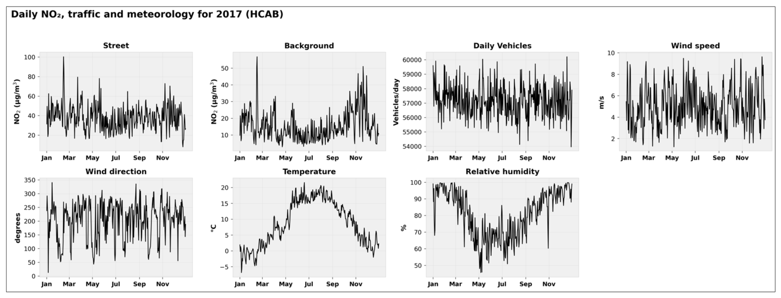
Figure A2.
Daily PM2.5, traffic, and meteorological variables for 2017 at HCAB. Layout follows Figure A1.
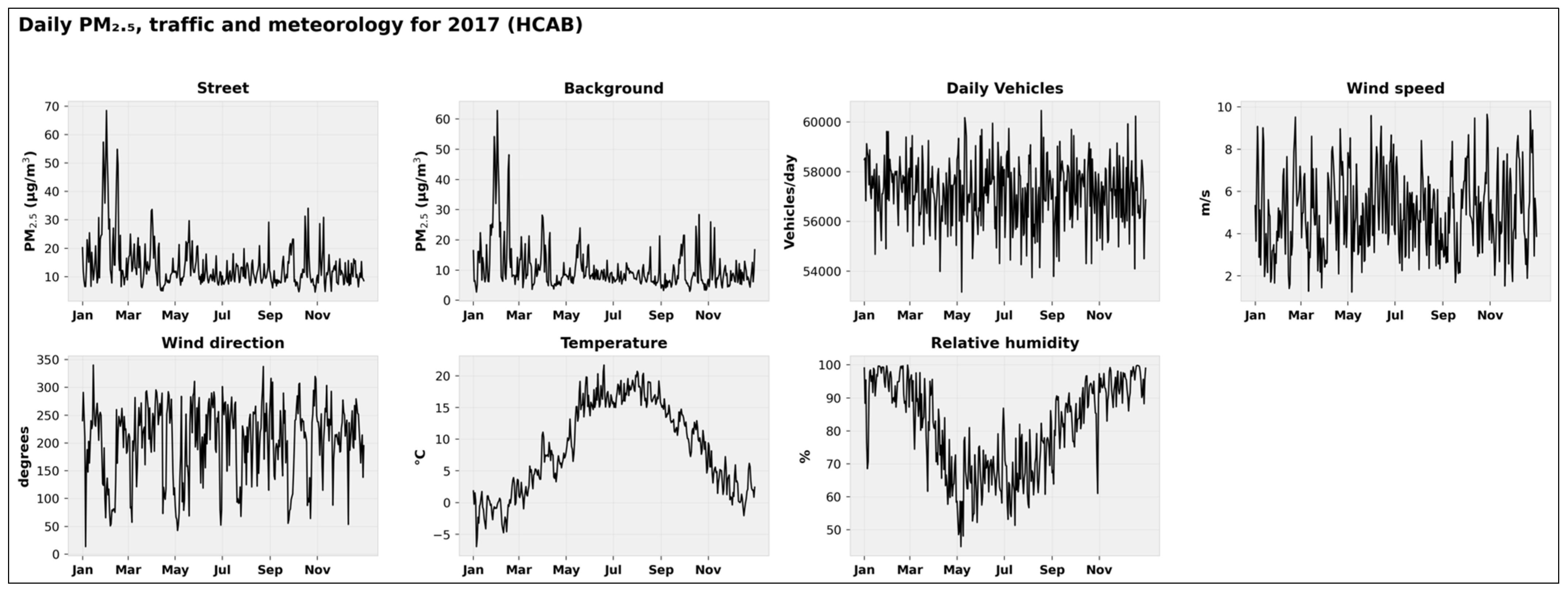
Figure A3.
Daily NO2, traffic, and meteorological variables for 2017 at JGTV. Layout follows Figure A1.
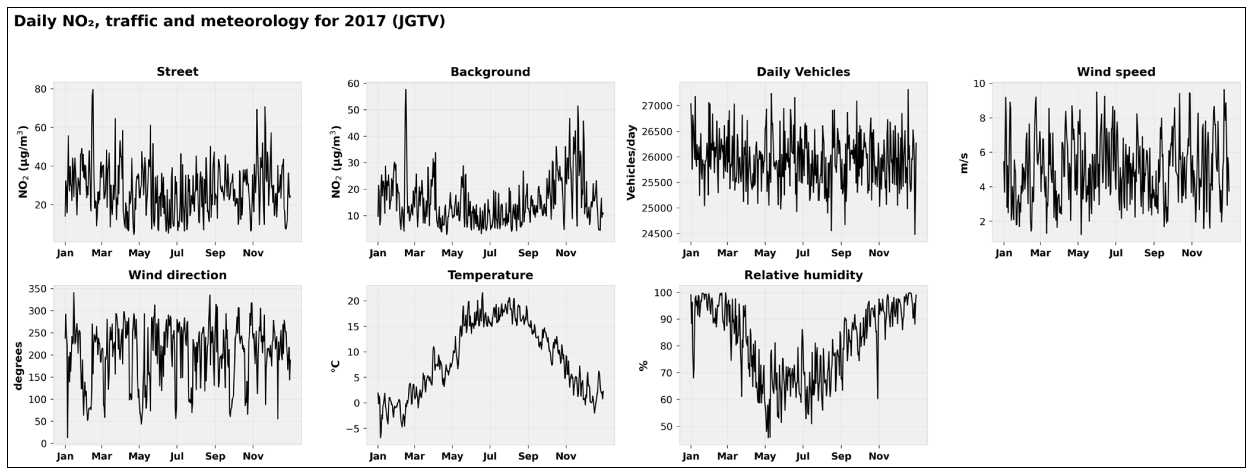
Figure A4 shows scatter density plots for all RF-based model configurations for the 2018 independent test year. The layout follows Figure 4, with rows corresponding to RF baseline (a–c), RF + 3D-Var (d–f), and RF + EKF (g–i), and columns corresponding to HCAB NO2, HCAB PM2.5, and JGTV NO2. The patterns are broadly consistent with the XGB results shown in Figure 4. The RF baseline shows slightly wider scatter than XGB, reflecting the modest performance gap between the two ML models discussed in Section 3.1. Both DA-corrected RF configurations show substantially tighter clustering around the 1:1 reference line, with RF + 3D-Var achieving marginally better performance than RF + EKF, consistent with the main text findings.
Figure A4.
Hexbin scatter density plots of observed versus modelled concentrations for the 2018 independent test year using Random Forest-based model configurations. Layout and notation follow Figure 5. Rows correspond to the RF baseline model (a–c), RF combined with 3D-Var data assimilation (d–f), and RF combined with the Extended Kalman Filter (g–i). Columns correspond to HCAB NO2 hourly concentrations (N = 8766), HCAB PM2.5 daily concentrations (N = 363), and JGTV NO2 hourly concentrations (N = 8766). The dashed line indicates the 1:1 reference. Performance metrics (RMSE, R2, MBE) are annotated in each panel in µg m−3.
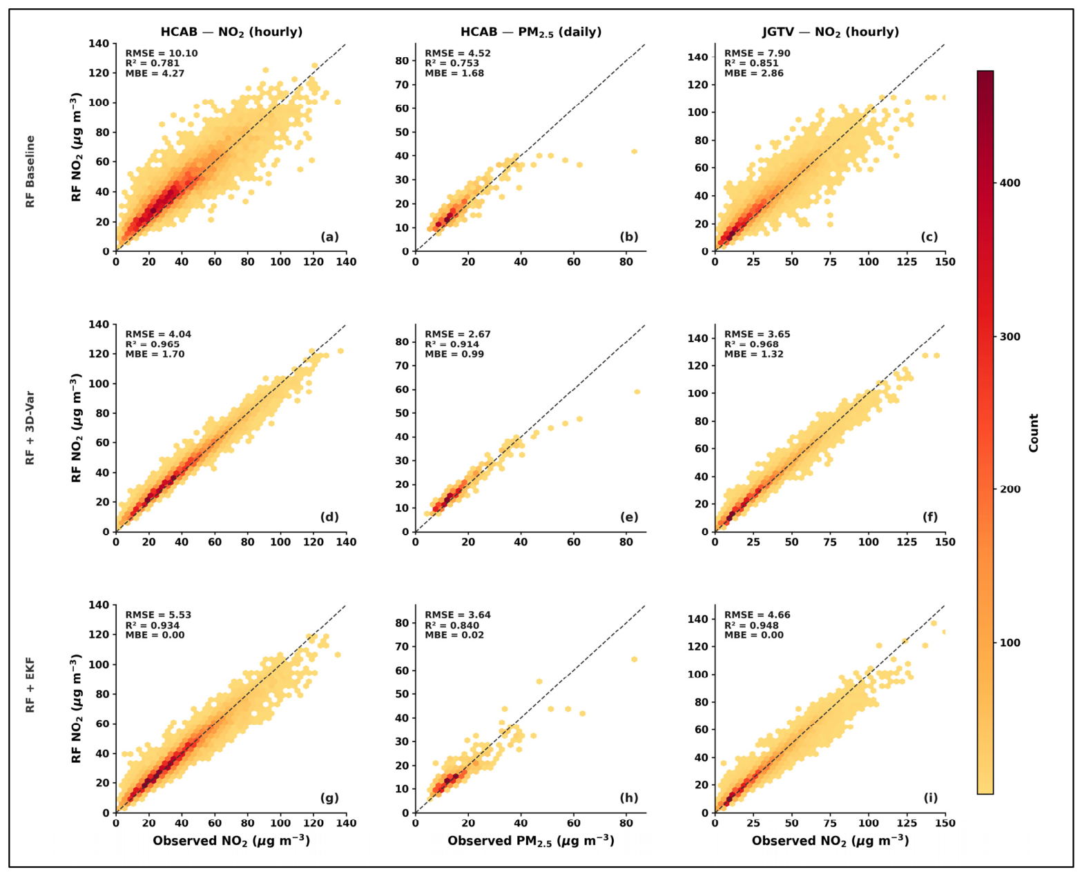
Figure A5 shows scatter density plots for all XGB-based model configurations for the 2017 validation year. Performance patterns are broadly similar to those observed in 2018, confirming that the results generalise across both evaluation years. The slightly lower scatter for some configurations in 2017 compared to 2018 reflects year-to-year differences in meteorological conditions and concentration distributions rather than any fundamental change in model behaviour.
Figure A5.
Hexbin scatter density plots of observed versus modelled concentrations for the 2017 validation year using XGBoost-based model configurations. Layout, notation, and axis scales follow Figure 5. Rows correspond to the XGB baseline model (a–c), XGB combined with 3D-Var data assimilation (d–f), and XGB combined with the Extended Kalman Filter (g–i). Columns correspond to HCAB NO2 hourly concentrations (N = 8766), HCAB PM2.5 daily concentrations (N = 363), and JGTV NO2 hourly concentrations (N = 8766). The dashed line indicates the 1:1 reference. Performance metrics (RMSE, R2, MBE) are annotated in each panel in µg m−3.
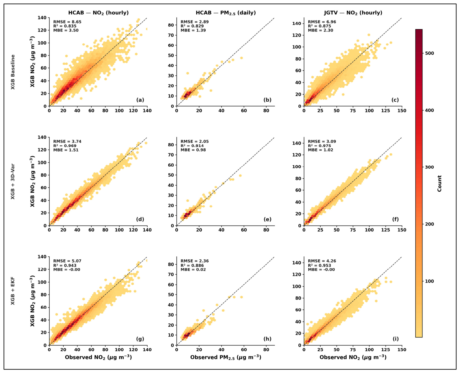
Figure A6 shows scatter density plots for all RF-based model configurations for the 2017 validation year, equivalent to Figure A5 for RF. The RF baseline shows modestly wider scatter than XGB in 2017, consistent with the 2018 results. Both DA methods produce comparable improvements relative to their respective RF baselines, with 3D-Var again outperforming EKF in terms of overall RMSE and R2, while EKF achieves near-zero MBE across all configurations.
Figure A6.
Hexbin scatter density plots of observed versus modelled concentrations for the 2017 validation year using Random Forest-based model configurations. Layout, notation, and axis scales follow Figure 5. Rows correspond to the RF baseline model (a–c), RF combined with 3D-Var data assimilation (d–f), and RF combined with the Extended Kalman Filter (g–i). Columns correspond to HCAB NO2 hourly concentrations (N = 8766), HCAB PM2.5 daily concentrations (N = 363), and JGTV NO2 hourly concentrations (N = 8766). The dashed line indicates the 1:1 reference. Performance metrics (RMSE, R2, MBE) are annotated in each panel in µg m−3.
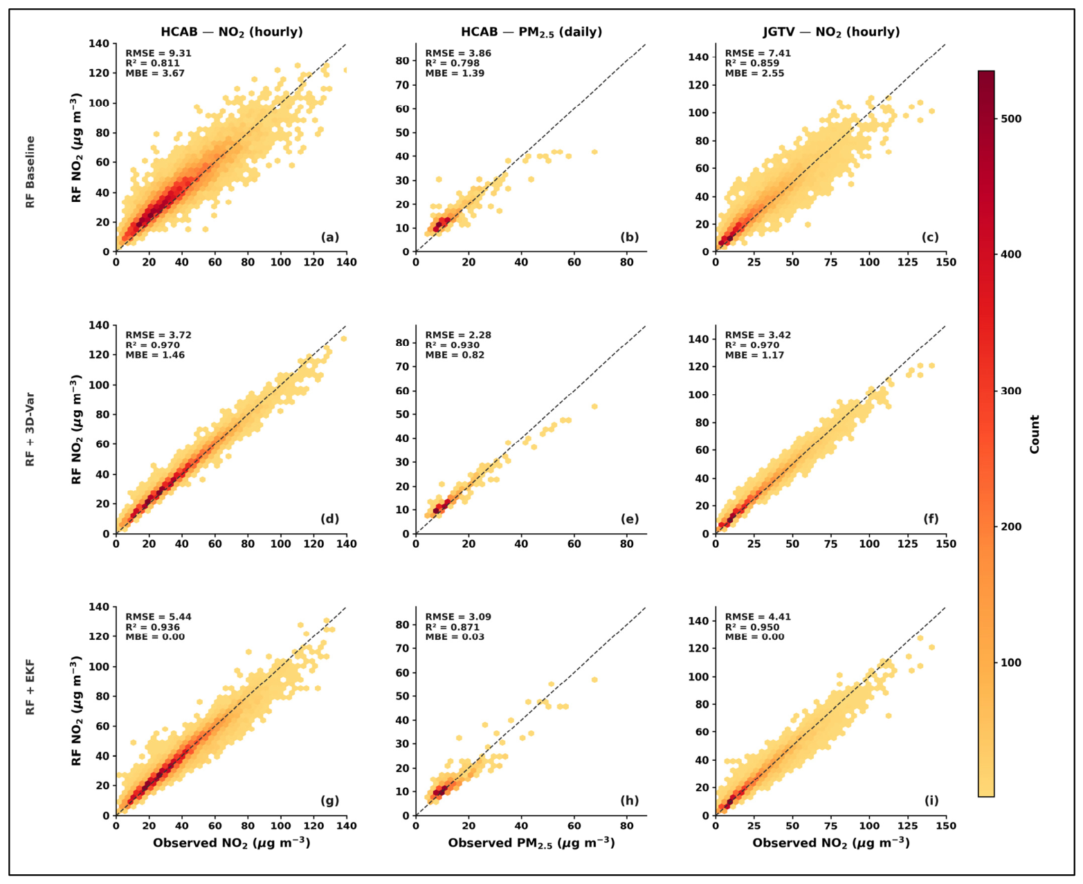
Figure A7 shows the case study time series for RF-based model configurations at HCAB NO2 during the 6 to 19 May 2018 episode. The RF baseline shows a similar pattern to the XGB baseline in Figure 6, with reasonable mean-level prediction but underestimation of individual spike magnitudes. RF + 3D-Var substantially reduces these errors, closely tracking the observed concentrations during spike periods. RF + EKF also improves on the baseline but shows the same lag behaviour at spike onset as its XGB equivalent, consistent with the sequential nature of the EKF correction.
Figure A7.
As in Figure 6, but using Random Forest-based model configurations. Panel (a) shows the observed HCAB NO2 data, while Panels (b), (c), and (d) show the RF baseline, RF + 3D-Var, and RF + EKF outputs, respectively. The thin dark grey line in each panel reproduces the observed record for reference. Amber shading indicates hours where observed NO2 exceeded 88.5 µg m−3.
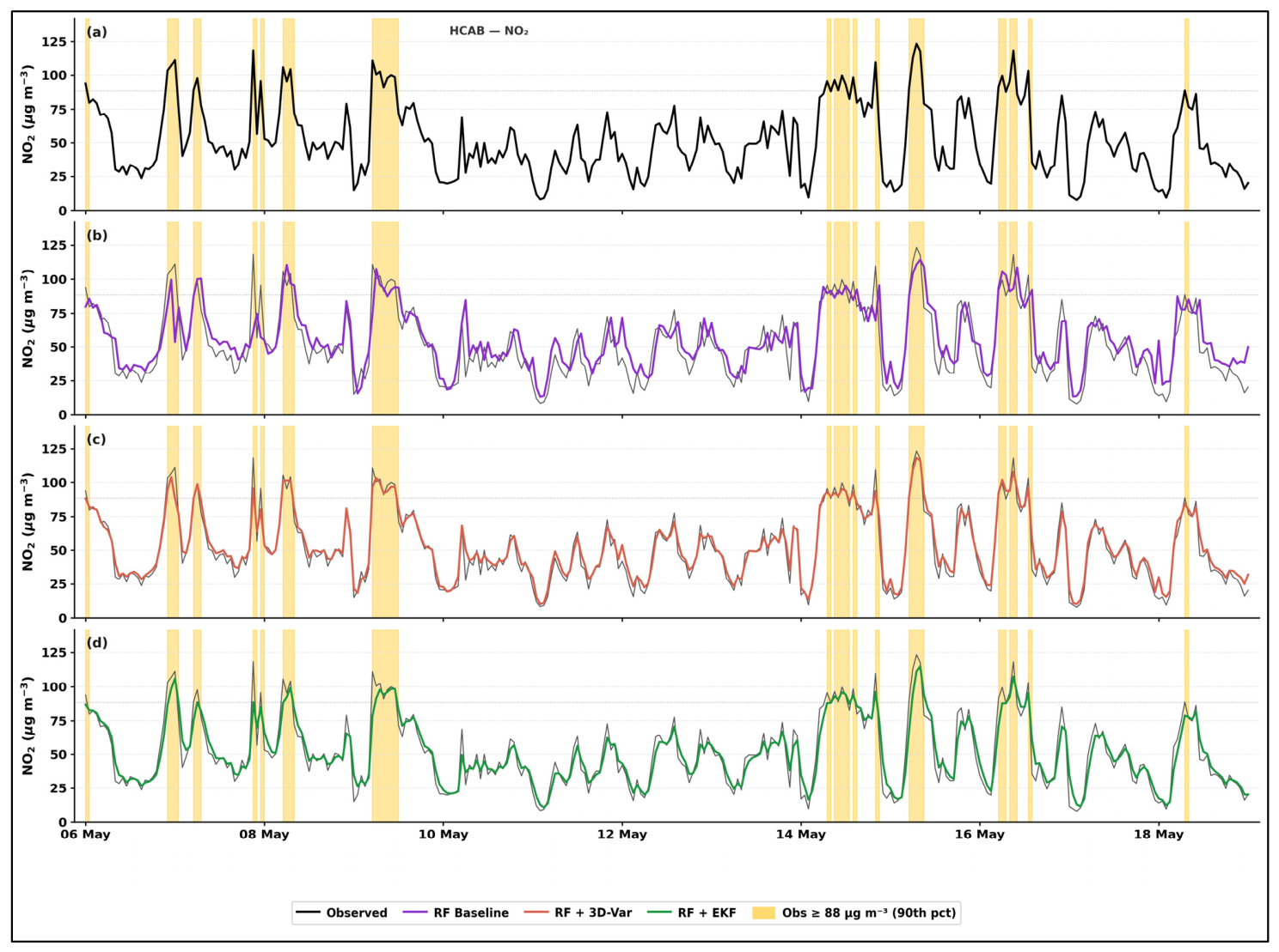
Figure A8 shows the case study time series for RF-based model configurations at HCAB PM2.5 during the same episode. As noted in Section 3.5, no PM2.5 observations exceed the spike threshold during this window. The RF baseline overestimates concentrations throughout, consistent with the positive MBE reported in Section 3.1. Both RF + 3D-Var and RF + EKF reduce this overestimation, with RF + 3D-Var achieving closer agreement with the observed daily pattern.
Figure A9 shows the case study time series for RF-based model configurations at JGTV NO2 during the same episode. The patterns are consistent with Figure 8 for XGB, with lower absolute concentrations than HCAB and fewer spike exceedances. RF + 3D-Var achieves the lowest errors during spike periods, while RF + EKF improves on the baseline but with a tendency to lag behind rapid concentration rises.
Figure A8.
As in Figure 7, but using Random Forest-based model configurations. Panel (a) shows the observed HCAB PM2.5 data while Panels (b), (c), and (d) show the RF baseline, RF + 3D-Var, and RF + EKF outputs, respectively. The thin dark grey line reproduces the observed record for reference. No observed PM2.5 concentrations exceeded the spike threshold (28.5 µg m−3) during this episode.
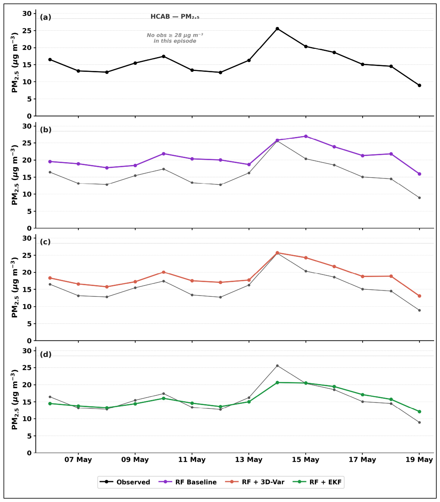
Figure A9.
As in Figure 8, but using Random Forest-based model configurations. Panel (a) shows the observed JGTV NO2 data, while Panels (b), (c), and (d) show the RF baseline, RF + 3D-Var, and RF + EKF outputs, respectively. The thin dark grey line reproduces the observed record for reference. Amber shading indicates hours where observed NO2 exceeded 75.8 µg m−3.
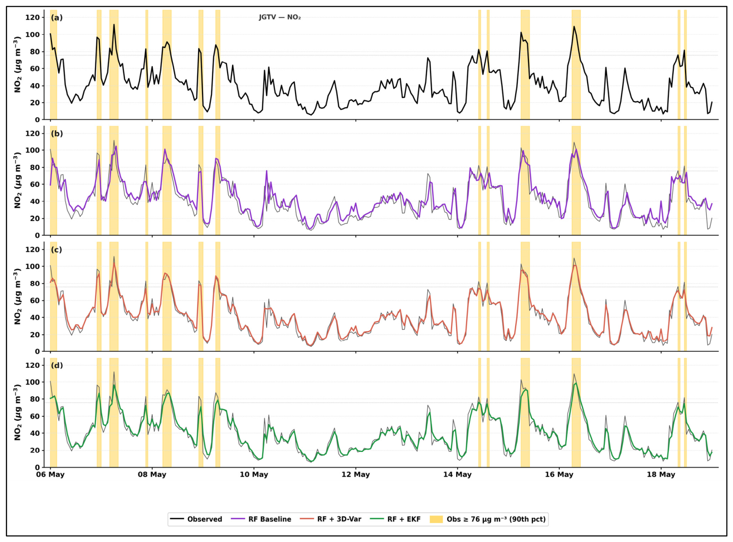
Figure A10 shows full-year time series for XGB-based model configurations for the 2017 validation year across all three pollutant-site combinations. The four rows correspond to observed concentrations, XGB baseline, XGB + 3D-Var, and XGB + EKF. The seasonal structure of NO2, higher in winter and lower in summer, is visible in all rows. The DA-corrected rows show notably tighter agreement with the observed record, particularly during winter months when concentrations are highest and baseline errors are largest. The dashed black line in the model rows reproduces the observed record as a visual reference.
Figure A10.
Full-year time series of observed and modelled concentrations for the 2017 validation year using XGBoost-based model configurations. Rows correspond to observed concentrations (a1–a3), XGB baseline (b1–b3), XGB + 3D-Var (c1–c3), and XGB + EKF (d1–d3). Columns correspond to HCAB NO2 hourly (left), HCAB PM2.5 daily (centre), and JGTV NO2 hourly (right). In panels (b1–b3), (c1–c3), and (d1–d3), the dashed black line reproduces the observed record as a visual reference. The dotted horizontal line in each panel marks the 90th percentile spike threshold (HCAB NO2: 88.5 µg m−3; HCAB PM2.5: 28.5 µg m−3; JGTV NO2: 75.8 µg m−3). The elevated PM2.5 concentrations visible in January–February 2017 reflect a genuine high-pollution episode observed at the HCAB site. Note that the XGB PM2.5 series contains N = 334 days due to outlier removal applied during preprocessing, compared to N = 365 for RF.
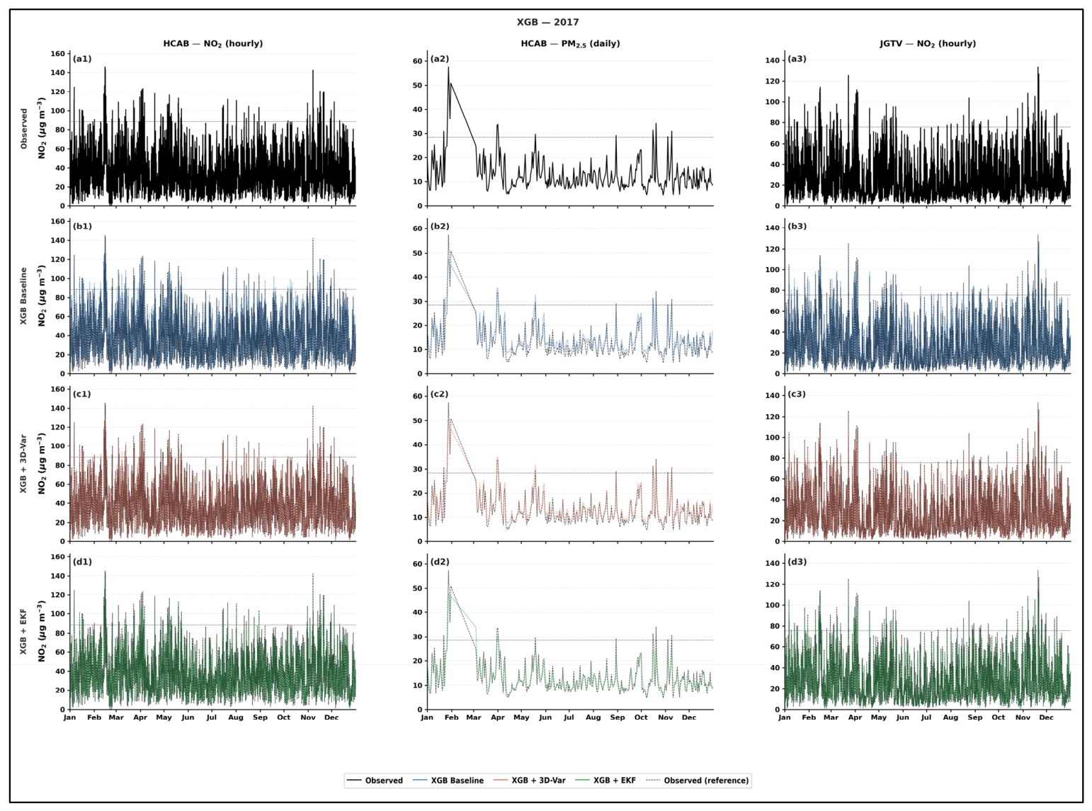
Figure A11 shows the full-year time series for XGB-based model configurations for the 2018 independent test year. The layout follows Figure A10. The seasonal patterns and the relative improvement from DA correction are consistent with those observed in 2017, confirming the generalisability of the results across both evaluation years. The January to February period shows elevated PM2.5 concentrations consistent with the high-pollution episode noted in Section 3.3.
Figure A11.
As in Figure A10, but for the 2018 independent test year using XGBoost-based model configurations. Rows correspond to observed concentrations (a1–a3), XGB baseline (b1–b3), XGB + 3D-Var (c1–c3), and XGB + EKF (d1–d3). Columns correspond to HCAB NO2 hourly (left), HCAB PM2.5 daily (centre), and JGTV NO2 hourly (right). The dashed black line in panels (b1–b3), (c1–c3), and (d1–d3) show the observed record for reference. Elevated PM2.5 concentrations are visible in January–February and October–November 2018, consistent with seasonal heating and stagnant atmospheric conditions typical of the Copenhagen urban environment.
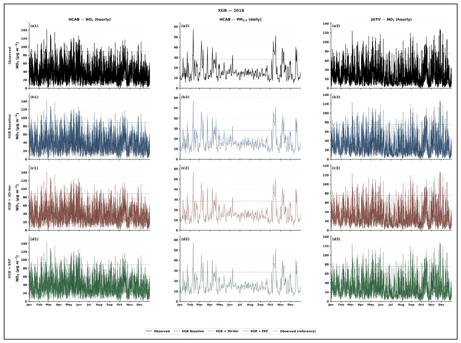
Figure A12 shows the full-year time series for RF-based model configurations for the 2017 validation year. The layout follows Figure A10. RF baseline errors are modestly larger than their XGB equivalents, consistent with the RMSE differences reported in Section 3.1. Both DA methods produce comparable improvements relative to the RF baseline, with 3D-Var again achieving lower overall errors than EKF.
Figure A12.
Full-year time series of observed and modelled concentrations for the 2017 validation year using Random Forest-based model configurations. Layout and notation follow Figure A10. Rows correspond to observed concentrations (a1–a3), RF baseline (b1–b3), RF + 3D-Var (c1–c3), and RF + EKF (d1–d3). The dashed black line in panels (b1–b3), (c1–c3), and (d1–d3) show the observed record for reference. The RF PM2.5 series contains N = 365 days, as no outlier removal was applied to the RF pipeline for this pollutant.
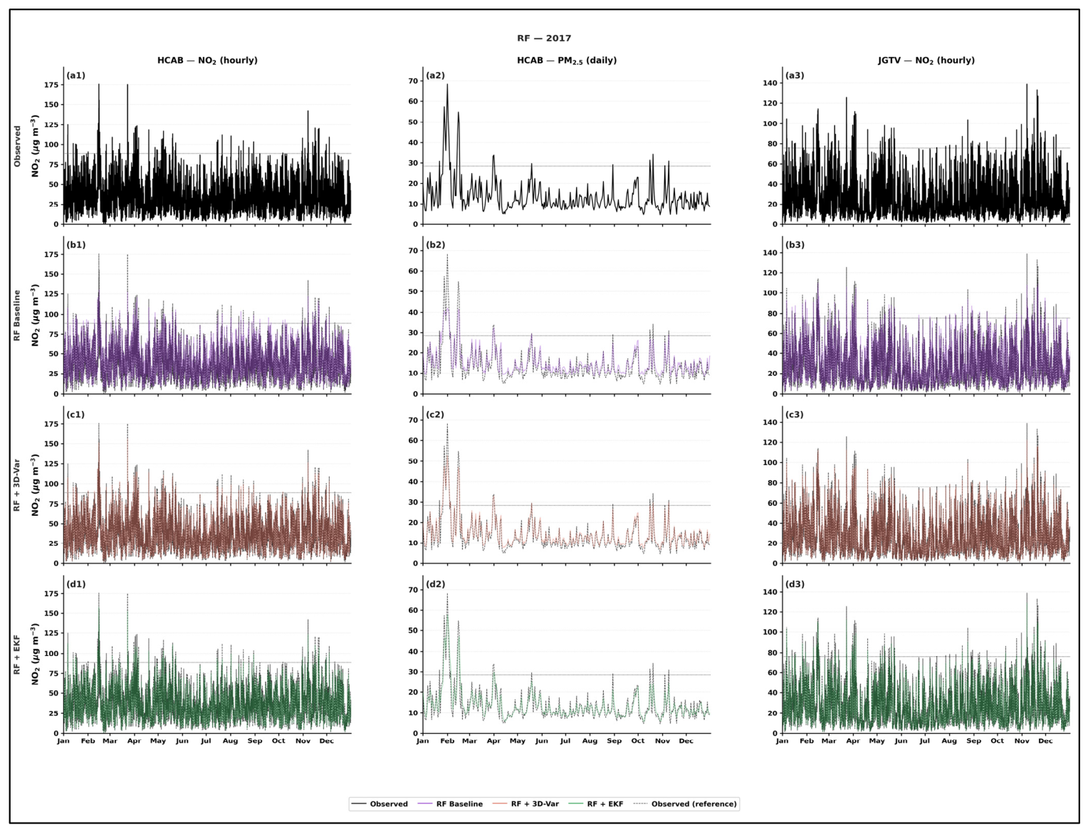
Figure A13 shows the full-year time series for RF-based model configurations for the 2018 independent test year. The layout follows Figure A10. The elevated PM2.5 concentrations visible in January to February 2018 reach higher peak values in the RF series compared to the XGB series, reflecting the retention of extreme values that were removed during XGB preprocessing. Both DA methods reduce errors throughout the year, with 3D-Var being the more effective correction across all three pollutant-site combinations.
Figure A13.
As in Figure A12, but for the 2018 independent test year using Random Forest-based model configurations. Rows correspond to observed concentrations (a1–a3), XGB baseline (b1–b3), XGB + 3D-Var (c1–c3), and XGB + EKF (d1–d3). Columns correspond to HCAB NO2 hourly (left), HCAB PM2.5 daily (centre), and JGTV NO2 hourly (right). The dashed black line in panels (b1–b3), (c1–c3), and (d1–d3) show the observed record for reference. The elevated PM2.5 episode visible in January–February 2018 reaches higher peak concentrations in the RF series compared to Figure A11, reflecting the retention of extreme values that were removed during XGB preprocessing.
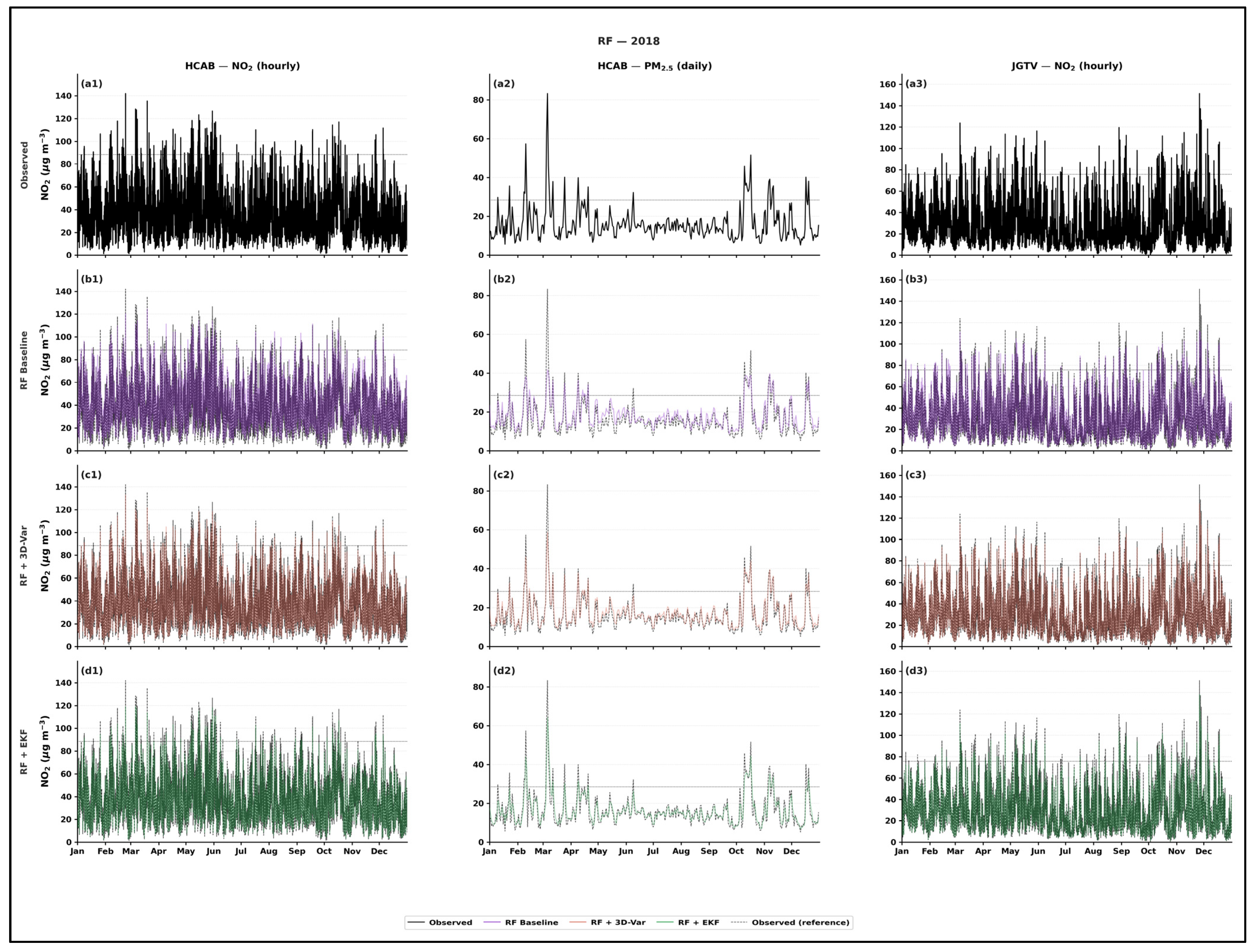
References
- European Commission. Directive (EU) 2024/2881 of the European Parliament and of the Council of 11 April 2024 on Ambient Air Quality and Cleaner Air for Europe. Official Journal of the European Union. 2024. Available online: https://eur-lex.europa.eu/legal-content/EN/TXT/?uri=CELEX%3A32024L2881 (accessed on 4 February 2026).
- World Health Organization. WHO Global Air Quality Guidelines: Particulate Matter (PM2.5 and PM10), Ozone, Nitrogen Dioxide, Sulfur Dioxide and Carbon Monoxide. 2021. Available online: https://www.who.int/publications/i/item/9789240034228 (accessed on 4 February 2026).
- Zhang, J.; Chen, G.; Wei, S.; Li, W.; Lip, G.Y.; Lin, H. Impact of air pollution and multimorbidity on the risk of incident atrial fibrillation. Heart 2025, 112, 318–325. [Google Scholar] [CrossRef] [Scilit] [PubMed]
- Zhang, Z.; Zhu, D.; Cui, B.; Ding, R.; Shi, X.; He, P. Association between particulate matter air pollution and lung cancer. Thorax 2020, 75, 85–87. [Google Scholar] [CrossRef] [Scilit] [PubMed]
- Pan, K.; Lin, F.; Huang, K.; Zeng, S.; Guo, M.; Cao, J.; Xi, Q. The effect of short-term exposure to air pollution on the admission of ischemic stroke and its interaction with meteorological factors. Public Health 2025, 239, 103–111. [Google Scholar] [CrossRef] [Scilit] [PubMed]
- European Environment Agency. Premature Deaths Due to Exposure to Fine Particulate Matter in Europe. 2024. Available online: https://www.eea.europa.eu/en/analysis/indicators/health-impacts-of-exposure-to (accessed on 4 February 2026).
- De Guzman, R.; Schiller, J. Air pollution and its impact on cancer incidence, cancer care and cancer outcomes. BMJ Oncol. 2025, 4, e000535. [Google Scholar] [CrossRef] [Scilit] [PubMed]
- Krecl, P.; Harrison, R.; Johansson, C.; Targino, A.; Beddows, D.; Ellermann, T.; Ketzel, M. Long-term trends in nitrogen oxides concentrations and on-road vehicle emission factors in Copenhagen, London and Stockholm. Environ. Pollut. 2021, 290, 118105. [Google Scholar] [CrossRef] [Scilit] [PubMed]
- Khan, J.; Kakosimos, K.; Raaschou-Nielsen, O.; Brandt, J.; Jensen, S.S.; Ellermann, T.; Ketzel, M. Development and performance evaluation of new AirGIS, a GIS based air pollution and human exposure modelling system. Atmos. Environ. 2019, 198, 102–121. [Google Scholar] [CrossRef] [Scilit]
- Taj, T.; Poulsen, A.H.; Ketzel, M.; Geels, C.; Brandt, J.; Christensen, J.H.; Raaschou-Nielsen, O. Long-term residential exposure to air pollution and Hodgkin lymphoma risk among adults in Denmark: A population-based case-control study. Cancer Causes Control 2021, 32, 935–942. [Google Scholar] [CrossRef] [Scilit] [PubMed]
- Kamara, A.; Harrison, R. Analysis of the air pollution climate of a central urban roadside supersite: London, Marylebone Road. Atmos. Environ. 2021, 258, 118479. [Google Scholar] [CrossRef] [Scilit]
- Lin, H.X.; Jin, J.; van den Herik, H.J. Air quality forecast through integrated data assimilation and machine learning. In Proceedings of the 11th International Conference on Agents and Artificial Intelligence, Prague, Czech Republic, 19–21 February 2019; SciTePress: Setúbal, Portugal, 2019; pp. 787–793. [Google Scholar] [CrossRef] [Scilit]
- Zaman, N.A.F.K.; Kanniah, K.D.; Kaskaoutis, D.G.; Latif, M.T. Evaluation of machine learning models for estimating PM2.5 concentrations across Malaysia. Appl. Sci. 2021, 11, 7326. [Google Scholar] [CrossRef] [Scilit]
- Muthukumar, P.; Cocom, E.; Nagrecha, K.; Comer, D.; Burga, I.; Taub, J.; Pourhomayoun, M. Predicting PM2.5 atmospheric air pollution using deep learning with meteorological data and ground-based observations and remote-sensing satellite big data. Air Qual. Atmos. Health 2022, 15, 1221–1234. [Google Scholar] [CrossRef] [Scilit] [PubMed]
- Zhalehdoost, A.; Taleai, M. Unravelling the importance of spatial and temporal resolutions in modeling urban air pollution using a machine learning approach. Sci. Rep. 2025, 15, 27708. [Google Scholar] [CrossRef] [Scilit] [PubMed]
- Su, Y. Prediction of air quality based on gradient boosting machine method. In Proceedings of the 2020 International Conference on Big Data and Informatization Education, Zhangjiajie, China, 24–26 April 2020; IEEE: Piscataway, NJ, USA, 2020; pp. 395–397. [Google Scholar] [CrossRef] [Scilit]
- Chen, Z.Y.; Zhang, T.H.; Zhang, R.; Zhu, Z.M.; Yang, J.; Chen, P.Y.; Guo, Y. Extreme gradient boosting model to estimate PM2.5 concentrations with missing-filled satellite data in China. Atmos. Environ. 2019, 202, 180–189. [Google Scholar] [CrossRef] [Scilit]
- Yagmur Aydin, N.; Aydin, I. Estimation of ground-level NO2 concentrations over megacities using Sentinel-5P and machine learning models: A case study of Istanbul. Int. Arch. Photogramm. Remote Sens. Spat. Inf. Sci. 2025, 48, 303–308. [Google Scholar] [CrossRef] [Scilit]
- Ding, W.; Qie, X. Prediction of air pollutant concentrations via random forest regressor coupled with uncertainty analysis—A case study in Ningxia. Atmosphere 2022, 13, 960. [Google Scholar] [CrossRef] [Scilit]
- Qin, X.; Huu, T.; Hofman, J.; Bonet, E.; Manna, V.; Deligiannis, N.; Philips, W. Fine-grained urban air quality mapping from sparse mobile air pollution measurements and dense traffic density. Remote Sens. 2022, 14, 2613. [Google Scholar] [CrossRef] [Scilit]
- Stafoggia, M.; Johansson, C.; Glantz, P.; Renzi, M.; Shtein, A.; de Hoogh, K.; Kloog, I.; Davoli, M.; Michelozzi, P.; Bellander, T. A random forest approach to estimate daily particulate matter, nitrogen dioxide, and ozone at fine spatial resolution in Sweden. Atmosphere 2020, 11, 239. [Google Scholar] [CrossRef] [Scilit]
- Sulaimon, I.; Alaka, H.; Olu-Ajayi, R.; Ahmad, M.; Ajayi, S.; Hye, A. Effect of traffic data set on various machine-learning algorithms when forecasting air quality. J. Eng. Des. Technol. 2022, 22, 1030–1056. [Google Scholar] [CrossRef] [Scilit]
- Gerges, F.; Llaguno-Munitxa, M.; Zondlo, M.; Boufadel, M.; Bou-Zeid, E. Weather and the city: Machine learning for predicting and attributing fine scale air quality to meteorological and urban determinants. Environ. Sci. Technol. 2024, 58, 6313–6325. [Google Scholar] [CrossRef] [Scilit] [PubMed]
- Cai, S.; Fang, F.; Tang, X.; Zhu, J.; Wang, Y. A hybrid data-driven and data assimilation method for spatiotemporal forecasting: PM2.5 forecasting in China. J. Adv. Model. Earth Syst. 2024, 16, e2023MS003789. [Google Scholar] [CrossRef] [Scilit]
- Méndez, M.; Merayo, M.G.; Núñez, M. Machine learning algorithms to forecast air quality: A survey. Artif. Intell. Rev. 2023, 56, 10031–10066. [Google Scholar] [CrossRef] [Scilit] [PubMed]
- Nguyen, C.V.; Soulhac, L. Data assimilation methods for urban air quality at the local scale. Atmos. Environ. 2021, 253, 118366. [Google Scholar] [CrossRef] [Scilit]
- Ma, X.; Liu, H.; Peng, Z. Improving WRF-Chem PM2.5 predictions by combining data assimilation and deep-learning-based bias correction. Environ. Int. 2025, 195, 109199. [Google Scholar] [CrossRef] [Scilit] [PubMed]
- He, X.; Zang, Z.; Li, Y.; Liu, N.; Hu, Y.; Liu, L.; You, W. Inversion of a near-real-time China gridded hourly SO2 emission inventory using deep learning combined with 3D-variational assimilation. Geophys. Res. Lett. 2025, 52, e2024GL114375. [Google Scholar] [CrossRef] [Scilit]
- Hermanns, A.; Lange, A.C.; Kowalski, J.; Fuchs, H.; Franke, P. Data clustering to optimise the representativity of observational data in air quality data assimilation: A case study with EURAD-IM (version 5.9.1 DA). EGUsphere 2025, 2025, 1–23. [Google Scholar] [CrossRef] [Scilit]
- Metia, S.; Nguyen, H.A.; Ha, Q.P. IoT-enabled wireless sensor networks for air pollution monitoring with extended fractional-order Kalman filtering. Sensors 2021, 21, 5313. [Google Scholar] [CrossRef] [Scilit] [PubMed]
- De Ridder, K.; Kumar, U.; Lauwaet, D.; Blyth, L.; Lefebvre, W. Kalman filter-based air quality forecast adjustment. Atmos. Environ. 2012, 50, 381–384. [Google Scholar] [CrossRef] [Scilit]
- Lu, X.; Sha, Y.H.; Li, Z.; Huang, Y.; Chen, W.; Chen, D.; Fung, J.C.H. Development and application of a hybrid long-short term memory–three dimensional variational technique for the improvement of PM2.5 forecasting. Sci. Total Environ. 2021, 770, 144221. [Google Scholar] [CrossRef] [Scilit] [PubMed]
- Huang, C.; Niu, T.; Wu, H.; Qu, Y.; Wang, T.; Li, M.; Li, R.; Liu, H. A data assimilation method combined with machine learning and its application to anthropogenic emission adjustment in CMAQ. Remote Sens. 2023, 15, 1711. [Google Scholar] [CrossRef] [Scilit]
- Tučkus, N.; D’Elia, I.; Chinnici, M.; Arcucci, R. Dynamic neural assimilation: A deep learning and data assimilation model for air quality predictions. Discov. Appl. Sci. 2024, 6, 176. [Google Scholar] [CrossRef] [Scilit]
- Zang, Z.; You, W.; Ye, H.; Liang, Y.; Li, Y.; Wang, D.; Yan, P. 3DVAR aerosol data assimilation and evaluation using surface PM2.5, Himawari-8 AOD and CALIPSO profile observations in the North China. Remote Sens. 2022, 14, 4009. [Google Scholar] [CrossRef] [Scilit]
- Lai, X.; Yang, T.; Wang, Z.; Chen, P. IoT implementation of Kalman filter to improve accuracy of air quality monitoring and prediction. Appl. Sci. 2019, 9, 1831. [Google Scholar] [CrossRef] [Scilit]
- Dai, Y.; Cai, X.; Zhong, J.; MacKenzie, A. Chemistry, street canyon geometry, and emissions effects on NO2 “hotspots” and regulatory “wiggle room”. npj Clim. Atmos. Sci. 2022, 5, 102. [Google Scholar] [CrossRef] [Scilit]
- Cheng, B.; Ma, Y.; Feng, F.; Zhang, Y.; Shen, J.; Wang, H.; Cheng, Y. Influence of weather and air pollution on concentration change of PM2.5 using a generalized additive model and gradient boosting machine. Atmos. Environ. 2021, 255, 118437. [Google Scholar] [CrossRef] [Scilit]
- Ellermann, T.; Nygaard, J.; Nøjgaard, J.K.; Nordstrøm, C.; Brandt, J.; Christensen, J.; Ketzel, M.; Massling, A.; Jensen, S.S. The Danish Air Quality Monitoring Programme. Annual Summary for 2017; Danish Centre for Environment and Energy: Roskilde, Denmark, 2018; Available online: http://dce2.au.dk/pub/SR281.pdf (accessed on 4 February 2026).
- Department of Environmental Science, Aarhus University. Measuring Stations. 2025. Available online: https://envs.au.dk/en/research-areas/air-pollution-emissions-and-effects/the-monitoring-program/measuring-stations (accessed on 4 February 2026).
- Wikipedia. H.C. Andersens Boulevard (Copenhagen, Denmark). 2025. Available online: https://da.wikipedia.org/wiki/H.C._Andersens_Boulevard (accessed on 4 February 2026).
- Department of Environmental Science, Aarhus University. Measuring Methods. 2025. Available online: https://envs.au.dk/en/research-areas/air-pollution-emissions-and-effects/the-monitoring-program/measuring-methods (accessed on 4 February 2026).
- Ellermann, T.; Nygaard, J.; Nøjgaard, J.K.; Nordstrøm, C.; Brandt, J.; Christensen, J.; Ketzel, M.; Massling, A.; Jensen, S.S. The Danish Air Quality Monitoring Programme. Annual Summary for 2018; Danish Centre for Environment and Energy: Roskilde, Denmark, 2020; Available online: https://dce2.au.dk/pub/SR360.pdf (accessed on 4 February 2026).
- Jensen, S.S.; Plejdrup, M.S.; Hillig, K. GIS-Based National Road and Traffic Database 1960–2020; Technical Report No. 151; Danish Centre for Environment and Energy, Aarhus University: Roskilde, Denmark, 2019; Available online: http://dce2.au.dk/pub/TR151.pdf (accessed on 4 February 2026).
- Scikit-Learn Developers. Isolation Forest Example. 2025. Available online: https://scikit-learn.org/stable/auto_examples/ensemble/plot_isolation_forest.html (accessed on 4 February 2026).
- Wikipedia. Isolation Forest. 2025. Available online: https://en.wikipedia.org/wiki/Isolation_forest (accessed on 4 February 2026).
- Scikit-Learn Developers. MinMaxScaler. 2025. Available online: https://scikit-learn.org/stable/modules/generated/sklearn.preprocessing.MinMaxScaler.html (accessed on 4 February 2026).
- Zhang, Z.; Johansson, C.; Engardt, M.; Stafoggia, M.; Ma, X. Improving 3-day deterministic air pollution forecasts using machine learning algorithms. Atmos. Chem. Phys. 2024, 24, 807–851. [Google Scholar] [CrossRef] [Scilit]
- Dash, U.K.; Park, S.Y.; Song, C.H.; Yu, J.; Yumimoto, K.; Uno, I. Performance comparisons of the three data assimilation methods for improved predictability of PM2.5: Ensemble Kalman filter, ensemble square root filter, and three-dimensional variational methods. Environ. Pollut. 2023, 322, 121099. [Google Scholar] [CrossRef] [Scilit] [PubMed]
- Djalalova, I.; Delle Monache, L.; Wilczak, J. PM2.5 analog forecast and Kalman filter post-processing for the Community Multiscale Air Quality (CMAQ) model. Atmos. Environ. 2015, 108, 76–87. [Google Scholar] [CrossRef] [Scilit]
- Wang, B.; Sun, Z.; Jiang, X.; Zeng, J.; Liu, R. Kalman filter and its application in data assimilation. Atmosphere 2023, 14, 1319. [Google Scholar] [CrossRef] [Scilit]
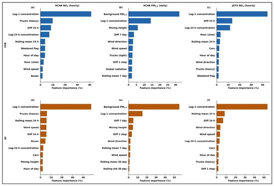
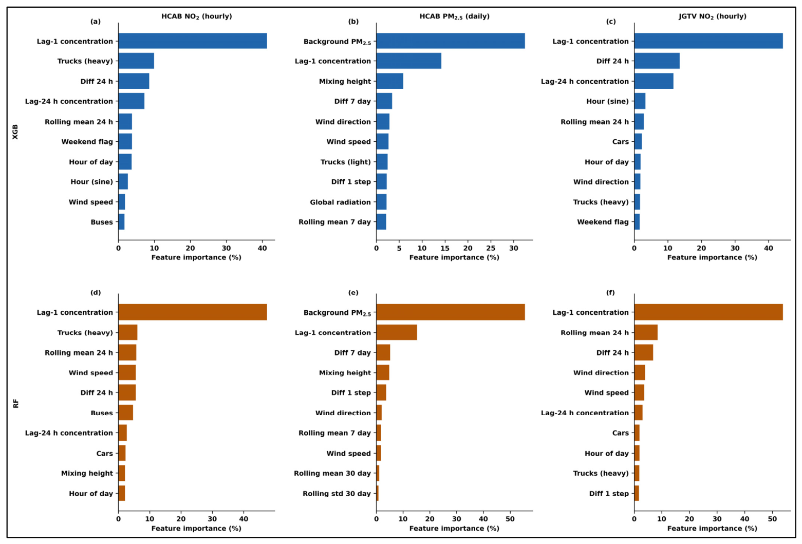

Disclaimer/Publisher’s Note: The statements, opinions and data contained in all publications are solely those of the individual author(s) and contributor(s) and not of MDPI and/or the editor(s). MDPI and/or the editor(s) disclaim responsibility for any injury to people or property resulting from any ideas, methods, instructions or products referred to in the content. |
© 2026 by the authors. Licensee MDPI, Basel, Switzerland. This article is an open access article distributed under the terms and conditions of the Creative Commons Attribution (CC BY) license.