Research on VLF Ionospheric Propagation Method Based on the Dynamic Stratification Transmission Matrix

Abstract

To address the poor computational efficiency of traditional fixed-stratification methods in very low frequency (VLF) ionospheric propagation modeling, this paper proposes a dynamic stratification algorithm. First, filtering optimization is applied to the electron density, and dynamic adaptive stratification is implemented in the vertical direction. By establishing a nonlinear mapping relationship between the electron density gradient and the stratification thickness, the algorithm integrates dynamic ionospheric stratification with a hybrid regularization algorithm for the transmission matrix. Specifically, Singular Value Decomposition (SVD) and dynamic truncation techniques are employed to process the transmission matrix, effectively resolving the numerical ill-posedness in regions with abrupt ionospheric changes. This enables high-precision calculation of reflection coefficients in the 3–30 kHz frequency band. By tuning parameters such as the reference stratification thickness and adjustment factors, an optimized stratification model and an algorithm quality evaluation coefficient are obtained. The simulation results demonstrate that, compared with fixed stratification, the proposed algorithm achieves an average relative error of 4.7% for the reflection coefficient in the VLF range while improving computational efficiency by more than 50%. This provides a promising approach for efficient and high-precision prediction of VLF wave propagation.

1. Introduction

Very low frequency (VLF, 3–30 kHz) electromagnetic waves exhibit unique propagation characteristics—enabling long-distance transmission over thousands of kilometers via the ionosphere-surface waveguides. They have long played an irreplaceable role in submarine communications, geological exploration, and space weather monitoring [1,2,3]. The interaction mechanism between VLF waves and the ionosphere is complex, where propagation characteristics significantly influenced by vertical gradient variations in the ionospheric electron density profile.

Since 1950, the layered ionospheric transmission matrix algorithm has undergone sustained development, becoming the core analytical method for addressing magnetoionic anisotropic propagation problems. In the 1920s, British physicist Oliver Heaviside and American scientist Arthur Kennelly first proposed the existence of the ionosphere, explaining long-distance radio propagation phenomena [4]. During the 1950s–1960s, Wait systematized VLF wave propagation theory by introducing waveguide mode theory, which treats the Earth’s surface and the ionosphere as waveguide boundaries within which VLF waves propagate via multiple modes, laying the theoretical groundwork for subsequent transmission matrix methods [5,6,7,8]. Early ionospheric models represented the ionosphere as a single or double layer (D region, E region), ignoring gradient variations, with VLF reflection dominated primarily by the low-altitude D region (60–90 km). Later, in the 1960s–1980s, Budden and Barron proposed treating the ionosphere as a layered medium and solving the boundary-matching problem of Maxwell’s equations in each layer using matrix methods [9]; Wait and Spies further developed a segmented homogeneous layered model of the ionospheric vertical profile, linking layer solutions through propagation matrices (or chain matrices) [10,11]. In 1971, Pappert et al. pioneered the use of matrix methods to compute VLF waveguide modes, improving computational efficiency and marking the shift from theoretical research to engineering applications [12]. Entering the 1980s–2000s, with advances in ionospheric sounding and the adoption of high-performance computing, researchers developed more refined ionospheric profile models and enhanced the computational efficiency and stability of numerical algorithms such as transmission matrices. Key developments included the introduction of the International Reference Ionosphere (IRI) [13,14,15], numerical optimizations of transmission matrix algorithms (e.g., impedance matrix method, adaptive layering) [16,17,18], hybrid algorithms combining transmission matrix with waveguide mode theory and parallel computing techniques [19,20], as well as satellite data assimilation and experimental validation [21,22]. These advances significantly improved the accuracy of VLF propagation prediction and provided reliable theoretical tools for fields such as space weather and lightning detection. From the 2000s to the present, as application scenarios have grown more complex, traditional models face limitations—such as neglecting abrupt terrain variations, equatorial anomaly gradient effects, and transient disturbances—making it difficult to handle rapidly evolving events like solar flares and geomagnetic storms [23,24]. Current VLF research is moving toward multi-physics coupling and real-time prediction, including integrating high-performance computing and artificial intelligence algorithms into transmission matrix modeling [25], refining the understanding of dynamic ionospheric disturbance mechanisms [26,27], and expanding into emerging application areas [28,29].

In summary, despite the progress made in the aforementioned studies, several unresolved issues remain in the VLF transmission matrix algorithms for ionospheric stratification. Current VLF transmission matrix algorithms predominantly employ fixed ionospheric stratification models for computation [30,31]; although existing studies have focused on enhancing computational efficiency and robustness [16,17,32], the coupling mechanism between dynamic ionospheric stratification strategies and transmission matrix algorithms remains unexplored. Moreover, no explicit correlation model has been established between the physical characteristics of ionospheric profiles and stratification thickness—for instance, the horizontal stratification thickness is typically fixed at 0.1–1 km without in-depth dynamic adjustment based on parameters such as electron density [30,33]. In addition, existing transmission matrix algorithms exhibit high computational complexity; they tend to display ill-posed characteristics in regions of sudden ionospheric parameter changes, leading to unstable numerical solutions [9,34], and the absence of certain predefined constraints results in slow iterative convergence.

To address these challenges, this paper proposes an optimized transmission matrix algorithm under dynamic stratification that incorporates ionospheric dynamic layering strategies into the VLF transmission matrix algorithms. By constructing a nonlinear mapping function between electron density gradients and stratification thickness, it achieves adaptive vertical stratification (dynamic densification or sparsification) and establishes a parametric correlation model linking electron density and stratification thickness. Subsequently, an SVD-regularized transmission matrix synthesis methodis designed to resolve the ill-posed numerical instability problem in the E–F region valley (approximately 120–150 km altitude), which is characterized by a local minimum in electron density and steep vertical gradients that pose numerical challenges for transmission matrix methods. Optimal parameter presets are determined through parameter sensitivity analysis (e.g., reference thickness, adjustment factors), balancing computational efficiency and accuracy to provide high-precision predictions of VLF propagation characteristics in complex ionospheric environments.

2. Theoretical Analysis

2.1. Dynamic Stratification Transmission Matrix Algorithm

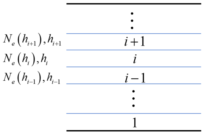
First, electron density gradient analysis is performed. The ionosphere is vertically stratified with fixed layers, where the center height of the i-th layer is denoted as hi (i = 1, 2, 3) and the corresponding electron density at that height is Ne(i), as shown in Figure 1.

The Savitzky–Golay filter [35] is employed to optimize the electron density data. Common methods for processing electron density data include statistical and moving average methods, digital filters, curve fitting, and functional modeling. Here, the Savitzky–Golay filtering method (hereinafter referred to as the S–G filtering method) is adopted to perform filtering and fitting on the electron density data sequence. The principle of the S–G filtering method involves performing polynomial least squares fitting within a sliding window. Its main advantage lies in effectively smoothing noise while preserving the local shape and peaks of the signal to the greatest extent possible. Moreover, it is relatively simple and computationally efficient, making it particularly suitable for data such as electron density profiles that contain both smoothly varying backgrounds and sharp peaks [36,37]. The fundamental formulation is as follows:

$${\widehat{N}}_e\left(i\right)={\displaystyle \sum _{k=-m}^m{c}_k\cdot N_e\left(i+k\right)}$$

(1)

where ${\widehat{N}}_e\left(i\right)$ is the filtered electron density value at height of h_i, c_k represents the filtering coefficients, determined by least squares fitting, which reflect the contribution weights of neighboring points to the current point, m is the half-window size (total number of points in the window = 2m + 1).

Subsequently, the central difference method is employed to obtain the electron density gradient as follows:

$$\nabla N_e\left(i\right)={\displaystyle \frac{{\widehat{N}}_e\left(i+1\right)-{\widehat{N}}_e\left(i-1\right)}{h_{i+1}-h_{i-1}}}$$

(2)

Then, physical constraints are imposed on the layer thickness. To ensure the physical plausibility of the numerical model, a constraint is applied to the minimum layer thickness. According to the plasma quasi-neutrality condition, the characteristic scale of the system should be much larger than the Debye length to maintain the quasi-neutrality assumption [38,39,40]. When the ionospheric stratification model is regarded as a continuum model, each layer should be treated as a fluid element satisfying the quasi-neutrality condition, and thus the layer thickness must be much greater than the Debye length. The Debye length is given by the following formula:

$${\lambda }_D=\sqrt{{\displaystyle \frac{{\epsilon }_0{k}_B{T}_e}{N_e{e}^2}}}$$

(3)

where ε₀ is the vacuum permittivity, k_B is the Boltzmann constant, T_e is the electron temperature, N_e is the electron density, e is the electron charge. When the layer thickness is three times to the Debye length, the electrostatic potential of Debye shielding is given by:

$$\varphi \left(3{\lambda }_D\right)\propto {\displaystyle \frac{1}{3{\lambda }_D}}{e}^{-3}\approx {\displaystyle \frac{1}{3{\lambda }_D}}\times 0.0498$$

(4)

This means that the perturbation potential has attenuated by approximately 95% at 3λ_D, indicating that the shielding effect is relatively complete from a physical perspective and the electrostatic influence can be neglected. Therefore, the minimum layer thickness is set to 3λ_D, we have:

$$d_{\min }=3{\lambda }_D=3\sqrt{{\displaystyle \frac{{\epsilon }_0{k}_B{T}_e}{N_e{e}^2}}}$$

(5)

In grid-based numerical methods such as the Finite-Difference Time-Domain (FDTD) method, it is necessary to reduce the artificial error introduced by numerical discretization—namely, numerical dispersion. It is generally required that the grid cell size of Δ is much smaller than the minimum wavelength of λ_min [41]. Based on the relationship between wavelength, frequency, and relative permittivity, we have:

$$\Delta \ll {\lambda }_{\min }={\displaystyle \frac{c}{f_{\max }\sqrt{{\epsilon }_r}}}$$

(6)

where c is the speed of light in vacuum, f_max is the maximum frequency, ε_r is the relative permittivity of the ionosphere.

According to the commonly adopted empirical rule [41,42,43], at least 10 sampling points per wavelength are ensured. Therefore, the maximum allowable thickness in this model is set to λ_min, yielding:

$$d_{\max }={\displaystyle \frac{{\lambda }_{\min }}{10}}={\displaystyle \frac{c}{10f_{\max }\sqrt{{\epsilon }_r}}}$$

(7)

In summary, the physical constraint range for the layer thickness is:

$$d_{\min }\le d_i\le d_{\max }$$

(8)

Next, the layer thickness is calculated. Traditional uniform layering presents inherent trade-offs between computational efficiency and accuracy, whereas adaptive mesh refinement (AMR) is a standard method to address such issues, whose core principle is to dynamically adjust the grid resolution according to the intensity of field quantity variations [44,45]. Following this general principle, this paper designs a gradient-driven adaptive layering strategy for the ionospheric electron density profile. This strategy is implemented through an exponential function to ensure that the layer thickness varies smoothly with the electron density gradient. The layer thickness follows the formula below:

$$d_i=d_0\cdot \exp \left(-\alpha \cdot \left|\nabla N_e\left(i\right)\right|\right)$$

(9)

where d₀ is the reference thickness and α is the adjustment factor that controls the sensitivity to the gradient; both parameters can be determined through numerical experiments combined with traditional empirical knowledge. This formula ensures that in critical regions with large electron density gradients (such as the F-region peak), thin layers (high resolution) are automatically adopted, while thick layers (low resolution) are used in regions with small gradients. This is consistent with the practice of using non-uniform grids in ionospheric modeling to capture rapid variations. This approach can be regarded as an application of physics-based mesh generation techniques to one-dimensional problems, achieving a smooth and continuous variation of grid size with the gradient through an exponential function.

2.2. Hybrid Regularization of Transmission Matrix

First, the single-layer transmission matrix is analyzed. Assume the ionospheric transmission matrix for the i-th is T_i (a 4 × 4 matrix). Tikhonov regularization [46,47] preprocessing is applied to Ti. In the modeling of electromagnetic wave propagation in the ionosphere based on the transmission matrix method, the stability of numerical computation and the physical plausibility of the solution are critical to ensuring model accuracy. In this paper, Tikhonov regularization preprocessing is introduced for the single-layer transmission matrix of T_i, primarily to address ill-posedness and ensure numerical stability.

The behavior of the ionospheric transmission matrix of T_i strongly depends on the local plasma parameters and the wave propagation characteristics. Under specific frequency and incidence angle conditions, the matrix of T_i^HT_i (where T_i^H denotes the conjugate transpose) may become ill-conditioned or even singular, characterized by an excessively high condition number or the presence of zero singular values. Directing to inverse of T_i^HT_i would render the numerical solution highly sensitive to small perturbations in the matrix elements and input parameters, thereby introducing significant numerical errors and potentially causing divergence in the computation process. To mitigate this issue, this study employs Tikhonov regularization to construct the preconditioning matrix T_i^pre:

$$T_i^{pre}={\left(T_i^H{T}_i+\gamma I\right)}^{-1}{T}_i^H$$

(10)

where γ is the regularization strength parameter and I is the identity matrix. The introduction of the regularization term of γI is equivalent to applying a positive shift to the singular value spectrum of T_i^HT_i. This significantly improves the condition number of the matrix, ensuring the numerical stability of its inversion, and enables the algorithm to maintain robustness even under complex ionospheric conditions.

To optimize the regularization effect, the regularization strength parameter γ is designed in conjunction with the physical characteristics of the model, adopting the following adaptive strategy:

$$\gamma ={\displaystyle \frac{{10}^{-3}}{\sqrt{d_i}}}$$

(11)

where d_i is the thickness of the i-th layer. This design enables the regularization strength to be dynamically adjusted according to the layer thickness: for thin layers (d_i is small), where the transmission matrix contributes relatively weakly to the overall solution, a smaller regularization strength is adopted to ensure solution accuracy; for thick layers (d_i is large), a stronger regularization constraint is applied to prioritize numerical stability. The coefficient 10⁻³ is determined by sensitivity analysis of the matrix condition number. When the regularization coefficient γ ranges from 10⁻⁴ to 10⁻², the condition number of the transmission matrix decreases from 10⁶ to 10², and the error in the reflection coefficient becomes stable. The value of 10⁻³ achieves an optimal balance between numerical stability and physical fidelity, and this parameter is universally applicable in the 3–30 kHz VLF band.

Then, SVD and dynamic truncation are performed. To further address the ill-conditioned behavior of the ionospheric transmission matrix preconditioning matrix of T_i^pre in transition layers such as the E–F region, and to ensure numerical stability, this paper further applies SVD and truncation to T_i^pre. The first step is to perform SVD decomposition on T_i^pre:

$$T_i^{pre}=U_i{\sum }_i{V}_i^H,{\sum }_i=diag\left({\sigma }_1,{\sigma }_2,{\sigma }_3,{\sigma }_4\right)$$

(12)

where U_i, V_i are the unitary matrix which satisfy to U_i*U_i^H = I and V_i*V_i^H = I; and ${\sum }_i$ is a diagonal matrix containing the singular values of ϭ_k (arranged in descending order).

A dynamic truncation threshold of ϭ_k(di) is set based on the layer thickness.

$${\sigma }_{th}\left(d_i\right)=\max \left({10}^{-4}{\sigma }_{\max },{\displaystyle \frac{d_0}{d_i}}\cdot {10}^{-5}{\sigma }_{\max }\right)$$

(13)

where σ_max is the maximum singular value obtained from the decomposition of the transmission matrix for the i-th layer, d₀ is the thickness of reference and d_i is the actual thickness of the i-th layer. This threshold design achieves a balance between stability and physical fidelity through two constraints, with parameter values validated by numerical sensitivity experiments. Specifically, the fixed base term 10⁻⁴σ_max provides a uniform lower bound for truncation across all layer thicknesses. A comparison of three truncation levels (10⁻³σ_max, 10⁻⁴σ_max, and 10⁻⁵σ_max) shows that 10⁻⁴σ_max effectively filters numerical noise, preventing matrix condition number deterioration caused by retaining excessively small singular values, while avoiding over-truncation of valid modes, thus ensuring the basic numerical stability and physical fidelity of the algorithm in thick layers. The dynamic adjustment term d_id₀⋅10⁻⁵σ_max introduces an inverse proportional relationship with layer thickness. When the ionospheric gradient changes sharply and the layer is automatically refined (d_i ≪ d₀), this term increases significantly, automatically raising the truncation threshold as the layer thickness decreases to adopt a more aggressive truncation strategy for thin layers. This design specifically targets numerically ill-conditioned thin layers such as the ionospheric E–F transition region, significantly improving the algorithm’s robustness in critical regions by actively filtering unstable high-frequency mode components. Taking the maximum of the two terms ensures that the truncation threshold is neither too low to be affected by noise nor too high to lose physical information, achieving adaptive regularization across the entire ionospheric altitude range.

Finally, all singular values smaller than the threshold σ_th(d_i) are set to zero to obtain the corrected singular value matrix ${\sum }_i^{reg}$, and the final regularized transmission matrix is reconstructed as:

$$T_i^{reg}=U_i{\sum }_i^{reg}{V}_i^H$$

(14)

The total transmission matrix of T_total is obtained by multiplying all regularized transmission matrices in sequence, from which the ionospheric reflection and transmission characteristics can be calculated.

$$T_{total}={\displaystyle \prod _{i=1}^N{T}_i^{reg}}$$

(15)

Here, N denotes the total number of vertical stratifications in the ionosphere.

2.3. Algorithm Quality Evaluation Function

In traditional transmission matrix algorithms for very low frequency (VLF) ionospheric propagation modeling, performance is often prioritized along a single dimension. For example, fixed stratification is adopted to simplify calculations and ensure engineering efficiency, at the expense of accuracy in regions with sharp electron density variations [48]; alternatively, overly fine stratification is used to enhance physical fidelity and reduce reflection coefficient calculation errors [49], while neglecting the impact of a sharp increase in computational load on real-time engineering applications (such as submarine communication link planning and space weather warnings). In essence, such approaches lack a synergistic consideration of the dual requirements of accuracy and efficiency.

To balance the relationship between physical accuracy and engineering efficiency in very low frequency (VLF) ionospheric propagation modeling, this paper defines an algorithm quality evaluation coefficient of Q to achieve a normalized quantitative evaluation of “accuracy–efficiency”. On one hand, this coefficient takes the average relative error of the reflection coefficient as the accuracy core, ensuring that the evaluation captures the essential physics of propagation; on the other hand, it incorporates the efficiency dimension by introducing the ratio of computation time and an efficiency weight coefficient, thereby avoiding a sharp drop in efficiency caused by excessive layer refinement in pursuit of higher accuracy. To objectively evaluate the quality coefficient of each algorithm, the computation time for fixed stratification with a uniform layer thickness of 1 km is taken as the time efficiency benchmark T_base. The calculation results from extremely fine fixed stratification with a uniform layer thickness of 0.1 km are defined as the reference true value R_ref of the reflection coefficient. For the algorithm to be evaluated, the quality evaluation coefficient Q is defined as:

$$Q=1-\left(\eta \cdot {\displaystyle \frac{T}{T_{base}}}+\left(1-\eta \right)\cdot \epsilon \right)$$

(16)

where T is the total computation time of the algorithm to be evaluated, η is the efficiency weight coefficient ranging from 0 to 1, which can be adjusted according to the preference between computational efficiency and accuracy in practical application scenarios. A larger η lays more stress on efficiency, whereas a smaller one attaches greater importance to accuracy. Specifically, η = 0.2 applies to engineering scenarios prioritizing accuracy with due consideration of efficiency, such as submarine communication and space weather early warning, and η = 0.8 is suitable for rapid prediction scenarios that prioritize efficiency and permit moderate errors.

To verify the robustness of the evaluation metric, this paper further performs sensitivity analysis. The results are shown in

Table 1. Quality evaluation coefficients for fixed and dynamic layering algorithms under different efficiency weight coefficients η.

η	Fixed-Layer Algorithm Q1	Dynamic-Layer Algorithm Q2
0	0.946	0.970
0.2	0.757	0.776
0.5	0.473	0.485
0.8	0.189	0.194
1	0	0

. When η = 1, the Q values of both algorithms are 0, because the evaluation completely ignores accuracy and only considers efficiency, while both algorithms have the same number of layers and computational efficiency, resulting in no difference. Under the remaining η values (η = 0, 0.2, 0.5, 0.8), the Q value of the dynamic layering algorithm is consistently higher than that of the fixed layering algorithm. The results demonstrate that the proposed algorithm achieves steady superiority under various trade-offs between accuracy and efficiency, exhibiting good universality.

ε is the mean relative error of the reflection coefficient, which is calculated as:

$$\epsilon ={\displaystyle \frac{1}{N}}{\displaystyle \sum _{i=1}^N\left|\frac{R_i-R_{ref}}{R_{ref}}\right|}$$

(17)

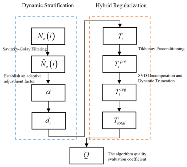
where N is the number of frequency sampling points. R_i is the reflection coefficient at the i-th frequency point; R_ref is the reference true value of the reflection coefficient. A larger value of the evaluation coefficient Q indicates better overall performance of the algorithm in terms of the “accuracy–efficiency” trade-off. The flowchart of the dynamic layering transmission matrix algorithm is shown in Figure 2.

3. Simulation and Validation

3.1. Algorithm Comparison

The algorithm in [31] has been proven to have reliable computational precision and accuracy within a propagation range of 2000 km for very low frequency (VLF) electromagnetic waves. This paper will conduct comparative calculations between Algorithm 2 (the proposed method) and Algorithm 1 (the method in [31]) within the same range of 2000 km, in order to verify the accuracy and efficiency of the proposed algorithm.

For clarity, the two algorithms compared in this section are defined as follows:

Algorithm 1 (Fixed-layer algorithm): The ionosphere is divided into fixed vertical layers with a uniform thickness of 1 km, and the classical transfer matrix algorithm as described in Ref. [31] is adopted.

Algorithm 2 (Proposed dynamic layering algorithm): The ionosphere is processed using the dynamic stratification method described in Section 2, with reference thickness d₀ = 1 km, adjustment factor α = 1.5, and hybrid regularization of the transmission matrix as described in Section 2.2).

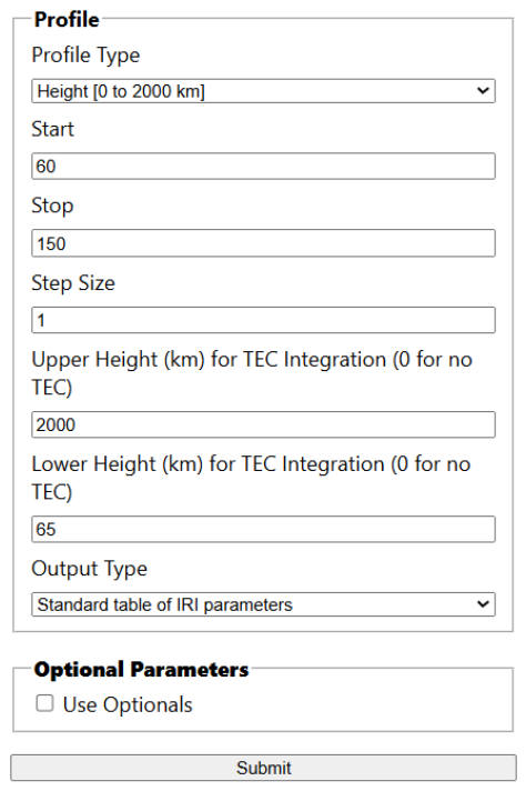
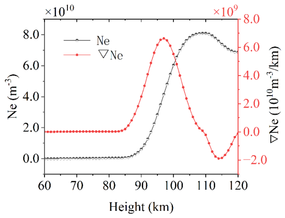
Using the International Reference Ionosphere (IRI-2020) model, ionospheric parameters were calculated for a mid-latitude region (29.0° N, 121.0° E) at 08:00 on January 1, 2024, representing winter daytime conditions under moderate solar activity (F10.7 = 131.2). The IRI-2020 model was configured with the following input parameters: geographic location (latitude 29.0° N, longitude 121.0° E), date (1 January 2024), time (08:00 local time), and solar activity level (F10.7 = 131.2). The output parameter extracted from IRI-2020 is the electron density profile N_e(h). The specific parameter settings include an altitude range of 60–120 km with a step size of 1 km. The frequency sweep ranges from 3 kHz to 30 kHz (VLF band) with a step size of 0.5 kHz, achieving full-band coverage. The date 1 January 2024 was chosen as a representative date for winter daytime conditions at mid-latitudes under moderate solar activity (F10.7 = 131.2), providing a baseline validation under quiescent ionospheric conditions without major solar or geomagnetic disturbances. The resulting ionospheric electron density and corresponding gradient are shown in Figure 3 and Figure 4.

Figure 4 shows that the electron density remains relatively stable in the D region (60–80 km). The maximum gradient in the D–E transition region (80–100 km) is $0.66\times {10}^{10}{\mathrm{m}}^{-3}/\mathrm{km}$, and the maximum gradient in the F layer (100–120 km) is $0.48\times {10}^{10}{\mathrm{m}}^{-3}/\mathrm{km}$. The maximum gradient in the D–E transition region is 1.4 times that in the F layer. The electron density varies significantly across different altitude ranges. Using the International Reference Ionosphere, specifically for the D layer (60–80 km), which plays a critical role in VLF wave attenuation and reflection, the 1 km sampling resolution ensures adequate capture of the steep vertical gradients in this region.

The traditional fixed-layer algorithm is compared with the dynamic layering algorithm proposed in this section. In the vertical fixed-layer method, the ionosphere is divided into fixed layers in the vertical direction, with a layer thickness of 1 km, and the classical transfer matrix algorithm [31] is adopted. In the dynamic layering transfer matrix algorithm, the reference thickness of d₀ is taken as 1 km and the adjustment factor of α is taken as 1.5. The ionosphere is processed with dynamic layering, and the original transfer matrix is subjected to hybrid regularization.

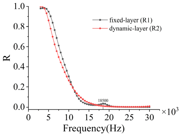
The results of the two algorithms are shown in Figure 5. When both the fixed layer thickness and the dynamic reference thickness are set to 1 km, Figure 5 shows that the reflection coefficients obtained by the two algorithms (since the polarization conversion effect of the ionosphere on VLF electromagnetic waves is not significant, only the reflection coefficients for the same polarization are considered) exhibit a high degree of agreement, consistent with theoretical expectations. Since the calculation results of the fixed-layer method have been proven to be reliable within this propagation range, it can be concluded that the calculation results of the dynamic layering algorithm are also reliable. It is particularly noteworthy that the reflection coefficient curve obtained with the fixed-layer method shows a small spurious fluctuation around 18.5 kHz, which may be caused by factors such as coherent superposition effects or numerical dispersion. In contrast, the dynamic layering algorithm eliminates this fluctuation, resulting in a smoother curve that better conforms to the actual wave propagation behavior.

To further comprehensively evaluate the performance of the two algorithms, the algorithm quality evaluation coefficient defined in Equation (16) is used for quantitative comparison. The mean relative error of Algorithm 1 is calculated to be 5.4%, and that of Algorithm 2 is 3.0%. In terms of computational efficiency, both algorithms have the same number of layers and their computation times are essentially identical. Taking an efficiency weight coefficient of η is 0.2, with emphasis on accuracy evaluation, the quality evaluation coefficient (Q₁) of Algorithm 1 is calculated to be 0.757, and that of Algorithm 2 (Q₂) is 0.776. The results show that the quality evaluation coefficient of the dynamic layering algorithm is significantly better than that of the fixed layering algorithm, verifying its advantage in comprehensive “accuracy–efficiency” performance.

3.2. Calculation Example

To verify the correctness of this method, we applied it to a practical example from reference [31] and compared the calculated results with both the measured statistical values collected during summer noontime over the past three years (2022–2024) and those from reference [31].

In this case, the latitude and longitude of the launch point are N37.38° and E112.12°, respectively, and those of the receiving point are N18.20° and E109.02°. The distance between the launch point and the receiving point is approximately 2000 km. The transmission power is 50 kW, the transmitting antenna efficiency is 40%, the frequency is 17 kHz, and the time is summer noon (12:00). This summer noontime case complements the winter daytime case presented in Section 3.1, providing validation under different seasonal conditions. We established observation points every 200 km within the range of 600–1600 km.

According to public reports, the propagation region of very-low-frequency electromagnetic waves can be roughly divided into three zones: the ground wave mode zone (0–400 km), the sky wave mode zone (400–1600 km), and the waveguide mode zone. In the sky wave propagation region, the dominant hop mode of electromagnetic waves is the one-hop mode.

The ionosphere exhibits non-uniformity in both the horizontal and vertical directions, but deriving and calculating while considering both aspects is challenging. Referring to the ionospheric statistical data from the ITU, we found that the non-uniformity of the ionosphere varies dramatically in the vertical direction, while it exhibits gradual variation in the horizontal direction. Therefore, we currently only consider the vertical non-uniformity of the ionosphere. Of course, this means that our algorithm cannot accurately calculate electromagnetic wave propagation over long distances. Based on our calculations and actual measurement experience, the current calculation results of our algorithm demonstrate acceptable accuracy within the range of 500–1600 km. The current validation is based on mid-latitude, daytime conditions (winter in Section 3.1 and summer in Section 3.2). The performance of the proposed algorithm under other geographic locations (e.g., equatorial, high-latitude), diurnal variations, and seasonal conditions requires further investigation.

3.2.1. Dynamic Layering Reference Thickness Selection

Reference [31] adopts a fixed ionospheric layering mode with a layer thickness of 1 km and a total of 60 layers. For the dynamic layering algorithm, the total number of layers N and the reference thickness of d₀ obey a power-law relationship $N\approx 61\cdot d_0^{-1.2}$, and its nonlinear scaling characteristic stems from an adaptive response to the electron density gradient. Compared with fixed layering, dynamic layering reduces the number of layers by 58% when d₀ = 3 km, while maintaining the ability to resolve key physical processes through local refinement in the transition region (layer thickness reduced to 1.2–1.8 km). The average relative error of the reflection coefficient over the entire frequency band is 4.7%, which still meets the accuracy requirement of ITU-R P.684 for VLF propagation models (error < 5%). Based on an error-cost trade-off analysis, it is recommended to select d₀ = 3 km as the optimal parameter value. Under this setting, the computational efficiency is improved by more than 50% while ensuring adequate resolution in the transition region.

3.2.2. Adjustment Factor Selection

According to the definition of Equation (9), the tuning factor α controls the sensitivity of the layer thickness to the electron density gradient: a larger α results in a finer layer thickness (smaller physical thickness) in regions with a large gradient; when α = 0, the method degenerates to a fixed-layer approach where the gradient does not affect the layer thickness.

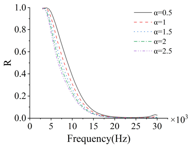
Figure 6 illustrates the influence of different adjustment factor α values on the variation of the reflection coefficient with frequency in the dynamic layering algorithm. It can be observed that for all α values, the reflection coefficient decreases monotonically with increasing frequency, which is consistent with the physical expectation for VLF wave propagation in the ionosphere (enhanced penetration at higher frequencies).

When α is between 0 and 1, the reflection coefficient curve is generally higher, particularly deviating significantly from the results for α = 1 in the low-frequency band (3–10 kHz). This is because an excessively small α leads to insufficient response of the layer thickness to the electron density gradient, resulting in inadequate refinement in regions with a large gradient, such as the D–E layer transition zone. This reduces the resolution of ionospheric parameter variations and produces a non-physical “over-reflection” artifact. When α is between 1 and 1.5, the curve converges to a reasonable range and transitions smoothly across the frequency band. Within this interval, the α value is sufficient to achieve adequate resolution in regions with a large gradient while avoiding numerical issues associated with excessive refinement, reflecting a good balance between accuracy and efficiency for the dynamic layering approach. When α exceeds 2, the reflection coefficient curve continues to shift downward, but the differences between the curves become very small, indicating that the calculation results tend toward stability.

When α is between 0 and 1, the reflection coefficient curves are generally higher, with a significant deviation from the mid-to-high frequency results especially in the low-frequency range (3–10 kHz), indicating that the algorithm insufficiently responds to the electron density gradient, leading to excessive reflection. When α is between 1 and 1.5, the curves converge to a reasonable range with smooth transitions across frequency bands, reflecting a balance between accuracy and efficiency achieved by dynamic layering. When α exceeds 2, the reflection coefficient is systematically reduced, possibly due to numerical dissipation introduced by excessive refinement in the transition region (overly small layer thickness).

The sensitivity analysis of α (Figure 6) demonstrates that the reflection coefficient of the dynamic layering algorithm is significantly regulated by the α value, with the optimal operating range being 1 < α < 1.5, where the reflection curves demonstrate good agreement with frequency monotonicity. Compared to α = 1.5, α = 1 achieves a comparable level of accuracy while requiring fewer total layers and higher computational efficiency. Therefore, a value of α = 1 is recommended for subsequent model development.

3.2.3. Calculation Result

To benchmark the proposed algorithm, the traditional ITU-R P.372-11 method is included for comparison. ITU-R P.372-11 is an internationally recognized recommendation for radio noise measurement and prediction, which provides empirical formulas for VLF propagation field strength estimation based on long-term statistical data. Although widely used in engineering practice due to its simplicity, this method does not account for the anisotropic and vertically inhomogeneous characteristics of the ionosphere, which limits its accuracy under complex ionospheric conditions. Therefore, comparing our dynamic stratification method against this traditional approach serves to demonstrate the advancement and necessity of the proposed model.

Table 2. Comparison of input parameters and model specifications for different methods.

Parameter	ITU-R P.372-11	Fixed-Layer Method [31]	Proposed Method
Ionospheric model	Empirical formula	IRI-2020	IRI-2020
Stratification strategy	Not applicable	Fixed (1 km)	Dynamic
Number of layers	Not applicable	60	Varies (reduced > 50%)
Frequency range	3–30 kHz	3–30 kHz	3–30 kHz
Anisotropy considered	No	Yes	Yes
Vertical non-uniformity	Not considered	Yes	Yes

summarizes the key parameters and model specifications for each method.

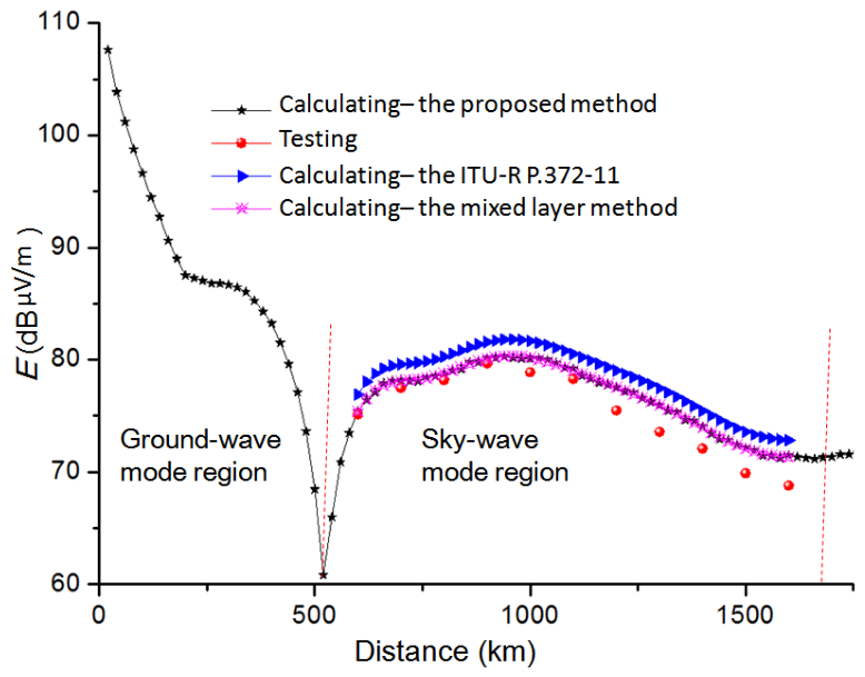
Figure 7 presents a comparison of sky-wave field strength values of VLF electromagnetic waves in the 500–1600 km range, obtained by different methods and actual measurements. In the figure, black stars represent the calculation results of the method proposed in this paper, pink stars represent the calculation results using the method from reference [31] (fixed layering algorithm), and blue triangles represent the values calculated by the traditional ITU-R P.372-11 method. The red dots in Figure 7 denote the measured statistical values in this area. Figure 7 shows that, compared with the measured data, the accuracy of the ionospheric layering matrix algorithm is much higher than that of the traditional ITU-R P.372-11 method. The results obtained by the proposed dynamic ionospheric layering method are in good agreement with those of the fixed ionospheric layering method, also demonstrating low efficiency high computational accuracy. Moreover, compared with the fixed layering method, the proposed method significantly reduces the number of layers, leading to a substantial improvement in computational efficiency, making it more suitable for engineering applications that require high-precision and complex ionospheric calculations.

4. Conclusions

From the perspective of balancing calculation accuracy and efficiency in engineering computations, this paper derives a dynamic layering matrix method for the ionosphere based on the full wave method, and establishes a more efficient anisotropic ionospheric model. Through calculation and verification, appropriate dynamic layering methods and rules for the ionosphere are determined. Comparative analysis results show that within the range of 500–1500 km, the calculation results obtained by the proposed method are in close agreement with measured data, providing a reliable reference for engineering calculations within this distance range. Moreover, compared with the fixed layering matrix method, the proposed method significantly improves computational efficiency. At present, because this method only considers the vertical non-uniformity of the ionosphere, it can ensure calculation accuracy within the 500–1500 km range. The proposed dynamic stratification method represents a step toward intelligent ionospheric modeling for radio applications, with potential integration with machine learning techniques for real-time VLF propagation prediction. Additionally, future work will systematically evaluate the algorithm’s performance under varying ionospheric conditions, including different latitudes, local times, and seasons. In future work, we will further improve the method by fully taking into account the horizontal non-uniformity of the ionosphere and the curvature of the Earth.

References

1. Rodger, C.J.; Werner, S.; Brundell, J.B.; Lay, E.H.; Thomson, N.R.; Holzworth, R.H.; Dowden, R.L. Detection efficiency of the VLF World-Wide Lightning Location Network (WWLLN): Initial case study. Ann. Geophys. 2006, 24, 3197–3214. [Google Scholar] [CrossRef]
2. Hayakawa, M. VLF/LF Radio Sounding of Ionospheric Perturbations Associated with Earthquakes. Sensors 2007, 7, 1141–1158. [Google Scholar] [CrossRef]
3. Barr, R.; Jones, D.L.; Rodger, C.J. ELF and VLF radio waves. J. Atmos. Sol.-Terr. Phys. 2000, 62, 1689–1718. [Google Scholar] [CrossRef]
4. Kennelly, A. On the Elevation of the Electrically Conducting Strata of the Earth Atmosphere. Electr. World Eng. 1902, 39, 473. [Google Scholar]
5. Wait, J.R. Electromagnetic Waves in Stratified Media; Pergamon Press: Oxford, UK, 1962. [Google Scholar]
6. Wait, J.R. Mode conversion and refraction effects in the Earth-ionosphere waveguide for VLF radio waves. J. Geophys. Res. 1968, 73, 3537–3548. [Google Scholar] [CrossRef]
7. Wait, J.R. On the mode theory of V.L.F. ionospheric propagation. Geofis. Pura E Appl. 1957, 37, 103–115. [Google Scholar]
8. Wait, J.R. On the theory of VLF propagation for a step model of the nonuniform earth–ionosphere wave guide. Can. J. Phys. 1968, 46, 1979–1983. [Google Scholar] [CrossRef]
9. Budden, K.G. The Propagation of Radio Waves: The Theory of Radio Waves of Low Power in the Ionosphere and Magnetosphere; Cambridge University Press: Cambridge, UK, 1988. [Google Scholar]
10. Wait, J.R. Characteristics of the earth-ionosphere waveguide for VLF radio waves. Radio Sci. 1964, 68D, 417–432. [Google Scholar]
11. Wait, J.R.; Spies, K.P. Height-Gain for VLF Radio Waves. Electromagn. Waves Stratif. Media 1970, 67D, 379–389. [Google Scholar] [CrossRef]
12. Pappert, R.A.; Snyder, R.R. Numerical Results for VLF Mode Conversion in the Earth-Ionosphere Waveguide. Radio Sci. 1971, 6, 239–254. [Google Scholar]
13. Bilitza, D. International Reference Ionosphere 1990. Planet. Space Sci. 1992, 40, 544. [Google Scholar]
14. Gulyaeva, T.L.; Titheridge, J.E. Advanced specification of electron density and temperature in the IRI ionosphere–plasmasphere model. Adv. Space Res. 2006, 38, 2587–2595. [Google Scholar] [CrossRef]
15. Reinisch, B.W.; Nsumei, P.; Huang, X.; Bilitza, D. Combining Satellite and Ground Observations for IRI-related Plasmasphere-Ionosphere Modeling. Adv. Space Res. 2006, 38, 2571–2578. [Google Scholar]
16. Pappert, R.A.; Ferguson, J.A. VLF/LF mode conversion model calculations for air to air transmissions in the earth-ionosphere waveguide. Radio Sci. 1986, 21, 551–558. [Google Scholar]
17. Ferguson, J.A.; Snyder, F.P. Approximate VLF/LF waveguide mode conversion model: Computer applications: FASTMC and BUMP. Radio Sci. 1980, 15, 975–985. [Google Scholar] [CrossRef]
18. Pan, W.Y. Propagation of Long, Very Long and Extremely Long Waves; University of Electronic Science and Technology of China Press: Chengdu, China, 2004. [Google Scholar]
19. Cummer, S.A. Lightning and Ionospheric Remote Sensing Using VLF/ELF Radio Atmospherics. Ph.D. Thesis, Stanford University, Redwood City, CA, USA, 1997. [Google Scholar]
20. Berenger, J.P. An effective FDTD scheme for the propagation of VLF-LF radiowaves in the Earth-Ionosphere waveguide. In Proceedings of the Radio Science Meeting, Memphis, TN, USA, 6–11 July 2014. [Google Scholar]
21. Nina, A.M.; Radovanović, M.M.; Milovanović, B.M.; Kovačević, A.; Bajčetić, J.; Popović, L.Č. Low ionospheric reactions on tropical depressions prior hurricanes. Adv. Space Res. 2017, 60, 1866–1877. [Google Scholar] [CrossRef]
22. Graf, K.L.; Lehtinen, N.G.; Spasojevic, M.; Cohen, M.B.; Marshall, R.A.; Inan, U.S. Analysis of experimentally validated trans-ionospheric attenuation estimates of VLF signals. J. Geophys. Res. Space Phys. 2013, 118, 2708–2720. [Google Scholar]
23. Kabirzadeh, R.; Marshall, R.A.; Inan, U.S. Early/fast VLF events produced by the quiescent heating of the lower ionosphere by thunderstorms. J. Geophys. Res. Atmos. 2017, 122, 7582–7593. [Google Scholar] [CrossRef]
24. Salut, M.M.; Cohen, M.B.; Ali, M.A.M.; Graf, K.L.; Cotts, B.R.T.; Kumar, S. On the Relationship Between Lightning Peak Current and Early VLF Perturbations. J. Geophys. Res. Atmos. 2013, 118, 7272–7282. [Google Scholar] [CrossRef]
25. Raissi, M.; Perdikaris, P.; Karniadakis, G.E. Physics-Informed Neural Networks: A Deep Learning Framework for Solving Forward and Inverse Problems Involving Nonlinear Partial Differential Equations. J. Comput. Phys. 2019, 378, 686–707. [Google Scholar] [CrossRef]
26. Pu, Y.; Chen, Y.; Dong, Y.; Zhang, K.; Wang, F.; Xi, X. Prediction of the Diurnal Variation of VLF Waves in Earth-Ionosphere Waveguide Based on BPNN-TL Method. IEEE Trans. Antennas Propag. 2025, 24, 38–42. [Google Scholar]
27. Hayakawa, M.; Kasahara, Y.; Nakamura, T.; Muto, F.; Horie, T.; Maekawa, S.; Hobara, Y.; Rozhnoi, A.A.; Solovieva, M.; Molchanov, O.A. A statistical study on the correlation between lower ionospheric perturbations as seen by subionospheric VLF/LF propagation and earthquakes. J. Geophys. Res. 2011, 115, A09305. [Google Scholar]
28. Hayakawa, M.; Hobara, Y. Current status of seismo-electromagnetics for short-term earthquake prediction. Geomat. Nat. Hazards Risk 2010, 1, 115–155. [Google Scholar]
29. Arriola, A.; Otiniano, L.; Vega, J.; Samanes, J. Development of a VLF receiver based on Red Pitaya for space weather studies. J. Atmos. Sol.-Terr. Phys. 2024, 260, 106–117. [Google Scholar] [CrossRef]
30. Yin, W.; Wei, B.; Zhang, S. Full-wave method for the analysis of the radiation characteristics of a VLF source in the atmosphere. Results Phys. 2019, 15, 102682. [Google Scholar] [CrossRef]
31. Zhao, L.; Zhan, Z.; Zhang, Z.; Feng, H. Analysis of VLF Electromagnetic Scattering in Lower Anisotropic Ionosphere Based on Transfer Matrix. Atmosphere 2024, 15, 1396. [Google Scholar] [CrossRef]
32. Lehtinen, N.; Inan, U. Emission of ELF/VLF Waves by a Modulated Electrojet upwards into the Ionosphere and into the Earth-Ionosphere Waveguide. In AGU Fall Meeting Abstracts; Wiley: Hoboken, NJ, USA, 2007. [Google Scholar]
33. Yang, J.; Li, Q.; Wang, J.; Hao, S. Influence of Artificial Ionospheric Disturbances on VLF Wave Propagation in Earth-Ionosphere Waveguide. Chin. J. Geophys. 2017, 60, 463–469. [Google Scholar]
34. Chen, J.; Yang, J.; Li, Q.; Yan, Y.; Hao, S.; Wang, C.; Wu, J.; Xu, B.; Xu, T.; Che, H.; et al. ELF/VLF Wave Radiation Experiment by Modulated Ionospheric Heating Based on Multi-Source Observations at EISCAT. Atmosphere 2022, 13, 228. [Google Scholar] [CrossRef]
35. Savitzky, A.; Golay, M.J.E. Smoothing and Differentiation of Data by Simplified Least Squares Procedures. Anal. Chem. 1964, 36, 1627–1639. [Google Scholar] [CrossRef]
36. Osei-Poku, L.; Tang, L.; Chen, W.; Chen, M. Evaluating Total Electron Content (TEC) Detrending Techniques in Determining Ionospheric Disturbances during Lightning Events in A Low Latitude Region. Remote Sens. 2021, 13, 4753. [Google Scholar] [CrossRef]
37. Ren, X.; Li, Y.; Mei, D.; Zhu, W.; Zhang, X. Improving topside ionospheric empirical model using FORMOSAT-7/COSMIC-2 data. J. Geod. 2023, 97, 30. [Google Scholar] [CrossRef]
38. Goldston, R.J. Introduction to Plasma Physics; CRC Press: Boca Raton, FL, USA, 2020. [Google Scholar]
39. Boyd, T.J.M.; Sanderson, J.J. The Physics of Plasmas; Cambridge University Press: Cambridge, UK, 2003. [Google Scholar]
40. Birdsall, C.K.; Langdon, A.B. Plasma Physics via Computer Simulation; CRC Press: Boca Raton, FL, USA, 2018. [Google Scholar]
41. Taflove, A.; Hagness, S.C.; Piket-May, M. Computational Electromagnetics: The Finite-Difference Time-Domain Method. In The Electrical Engineering Handbook; CRC Press: Boca Raton, FL, USA, 2005; pp. 629–670. [Google Scholar]
42. Wang, L.X.; Chen, J.; Mou, C.H. Hybrid optimization algorithm of FDTD/TDPO based on sparse sampling. Chin. J. Radio Sci. 2024, 39, 846–851. [Google Scholar] [CrossRef]
43. Wei, B.; Dong, Y.; Wang, F.; Li, C.Z. A Modified Node Algorithm for Dispersive Thin Layers Based on Shift Operator Finite-Difference Time-Domain Method. Acta Phys. Sin. 2010, 59, 2443–2450. [Google Scholar]
44. Lalgudi Gopalakrishnan, G.; Schmidt, M. Ionospheric Electron Density Modelling Using B-Splines and Constraint Optimization. Earth Planets Space 2022, 74, 143. [Google Scholar] [CrossRef]
45. Berger, M.J.; Colella, P. Local Adaptive Mesh Refinement for Shock Hydrodynamics. J. Comput. Phys. 1989, 82, 64–84. [Google Scholar] [CrossRef]
46. Morozov, V.A. Regularization of incorrectly posed problems and the choice of regularization parameter. USSR Comput. Math. Math. Phys. 1966, 6, 242–251. [Google Scholar] [CrossRef]
47. Willoughby, R.A. Solutions of ill-posed problems (AN Tikhonov and VY Arsenin). Siam Rev. 1979, 21, 266. [Google Scholar] [CrossRef]
48. Ma, X.; Yan, W.; Hu, Z.; Yuan, J.; Yang, C.; Zhou, X.; Hua, Y.; Li, S. Phase Variation Model of VLF Timing Signal Based on Waveguide Mode Theory. Electronics 2025, 14, 2885. [Google Scholar] [CrossRef]
49. Meng, X.; Qiu, S.; Ji, Y. Grounded electrical source ground–airborne transient electromagnetic modelling with fictitious wave field methods. J. Earth Syst. Sci. 2020, 129, 130. [Google Scholar] [CrossRef]
Figure 1. Schematic diagram of ionospheric layering.
Atmosphere 17 00648 g001
Figure 2. The schematic diagram of the dynamic stratification transmission matrix algorithm.
Atmosphere 17 00648 g002
Figure 3. Data export interface of the IRI-2020 model.
Atmosphere 17 00648 g003
Figure 4. Electron density and its gradient variation in the ionosphere (60–120 km) over a specific region.
Atmosphere 17 00648 g004
Figure 5. Reflection coefficient versus frequency curves under fixed-layer and dynamic-layer algorithms.
Atmosphere 17 00648 g005
Figure 6. Reflection coefficient versus frequency curves under different tuning factors.
Atmosphere 17 00648 g006
Figure 7. Comparison between theoretical calculations and actual measurement statistics at noon (12:00) in summer with a frequency of 17 kHZ.
Atmosphere 17 00648 g007