


Abstract
Glacial ice cores are evidence of past environmental conditions through gases and particulate matter trapped within the drilled material. The Central Andes in the South American region are highly sensitive to climate changes; a long record of temperature and precipitation variability can be found in relation to massive ice caps. Available oxygen isotope data from three glacial ice cores from Nevados Sajama, Huascaran and Illimani (Peru and Bolivia) drilled over the last decades in the Central Andes are revisited to investigate climate variability over the past seven millennia, a period characterized globally by remarkable climatic stability. The analysis revealed statistically significant millennial- and centennial-scale periodicities in the isotope records ranging from centennial to millennial timescales. These cycles have periods of 1.3, 0.87, 0.67, 0.46, and 0.25 kiloyears (ka). A series of regional temperature minima and maxima are also identified. This variability in the Andean climate during the mid and late Holocene is interpreted as being strongly controlled by changes in solar activity, in particular, the forcing of “grand solar minima” is recognized. Likewise, less frequent climate changes could be correlated with Bond cycles and increased or decreased activity of the Atlantic Meridional Overturning Circulation (also known as AMOC or the thermohaline), among other climate forcings such as volcanic activity.
1. Introduction
Recent studies highlight the alarming rate at which Andean glaciers are retreating. Estimates indicate that the retreat rates are approximately 35% higher (0.7 m per year) retreat than the global average over the last decade [1]. Caro et al. [2] showed an increase of 12% in annual glacier melt in the Andean catchments driven by a 0.4 °C increase in temperature and a 9% reduction in precipitation. This rapid loss underscores the urgency of understanding past climate patterns to improve projections of future change.
The Central Andes of South America have experienced significant climatic shifts during the Holocene period [3,4,5]. Lacustrine sediment cores have revealed aridity and precipitation changes in the Central Andes, suggesting that climate variability plays a major role occurring at centennial to millennial timescales [6,7].
These phenomena are also well documented in glacial ice cores drilled at high elevations, where no significant anthropogenic influences have occurred and representative regional climatic conditions, particularly temperature, are preserved. The trapped air bubbles and particulate matter within the ice cores preserve a record of past gas variability [8] or even anthropic activities [9]. The water content of each layer in the ice cores could have an amount of stable isotopes (18O and deuterium, D) which preserve representative regional atmospheric conditions [10,11].
Thirty years of proxy data in the Central Andes have shed light on key aspects of regional climate evolution at the end of the Pleistocene and the Pleistocene–Holocene transition [12,13,14], as well as during the last millennia (e.g., Eichler et al. [15]). This research suggests that the Holocene and Pleistocene evolution was related to abrupt climate changes, particularly significant changes in temperature and precipitation.
However, the results obtained for these time intervals have led to limited attention to the more recent part of the record, particularly the interval between 7000 years BP (Before Present) and the last two millennia. While many studies address the possible causes of the cold periods from 8.2 to 7.5 ka (onset of the mid Holocene) [16,17,18], the period following 7.5 ka has received relatively little attention in the scientific literature. This interval, characterized by relative climatic stability on a global scale, exhibits significant variability in the stable isotope records of Andean glacial ice. This variability may have influenced the rise and fall of ancient civilizations in South America during the mid and late Holocene [19,20], or ecological changes such as glacier advances and retreats [21].
By reviewing the stable isotope data series with statistical techniques, such as the Lomb–Scargle spectral analysis [22], hidden periodicities and variability of the so-called “stable interval” of the mid and late Holocene can be analyzed. Lomb–Scargle periodogram has proven to be effective in the analysis of climate patterns [23,24] linking modern meteorological periodicities to regional atmospheric configurations.
The aim of this work is to re-analyze the palaeoclimate variability based on the available data. Specifically, this study reconstructs the palaeotemperatures since the last 7 ka The mid- and late-Holocene climate variability is therefore inferred from stable oxygen isotope stratigraphy in three ice cores drilled in the Central Andes of Peru and Bolivia (two based on δ18O and one on deuterium δD). The three ice cores are representative of Andean summits, where temperature and precipitation are consistently low. These ice records have been previously reviewed by Ramirez et al. [14] who analyzed the Pleistocene–Holocene interval. They reported similar climate variability of at least two of the cores, Nevado Huascarán and Nevado Illimani, whereas Nevado Sajama reflects more localized conditions influenced by humid phases, at least for the Pleistocene period.
Some novel aspects can be derived from reviewing the three ice cores. Despite differences in elevation, accumulation rates, and local climatic influences, the Illimani, Sajama, and Huascarán cores exhibit coherent multi-centennial to millennial-scale temperature variability during the last 7 ka during periods of reduced humidity at Nevado Sajama.
Study Area
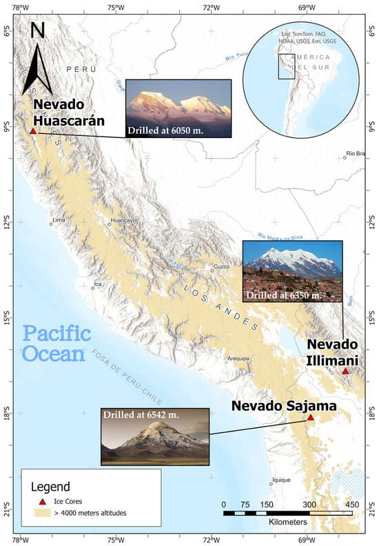
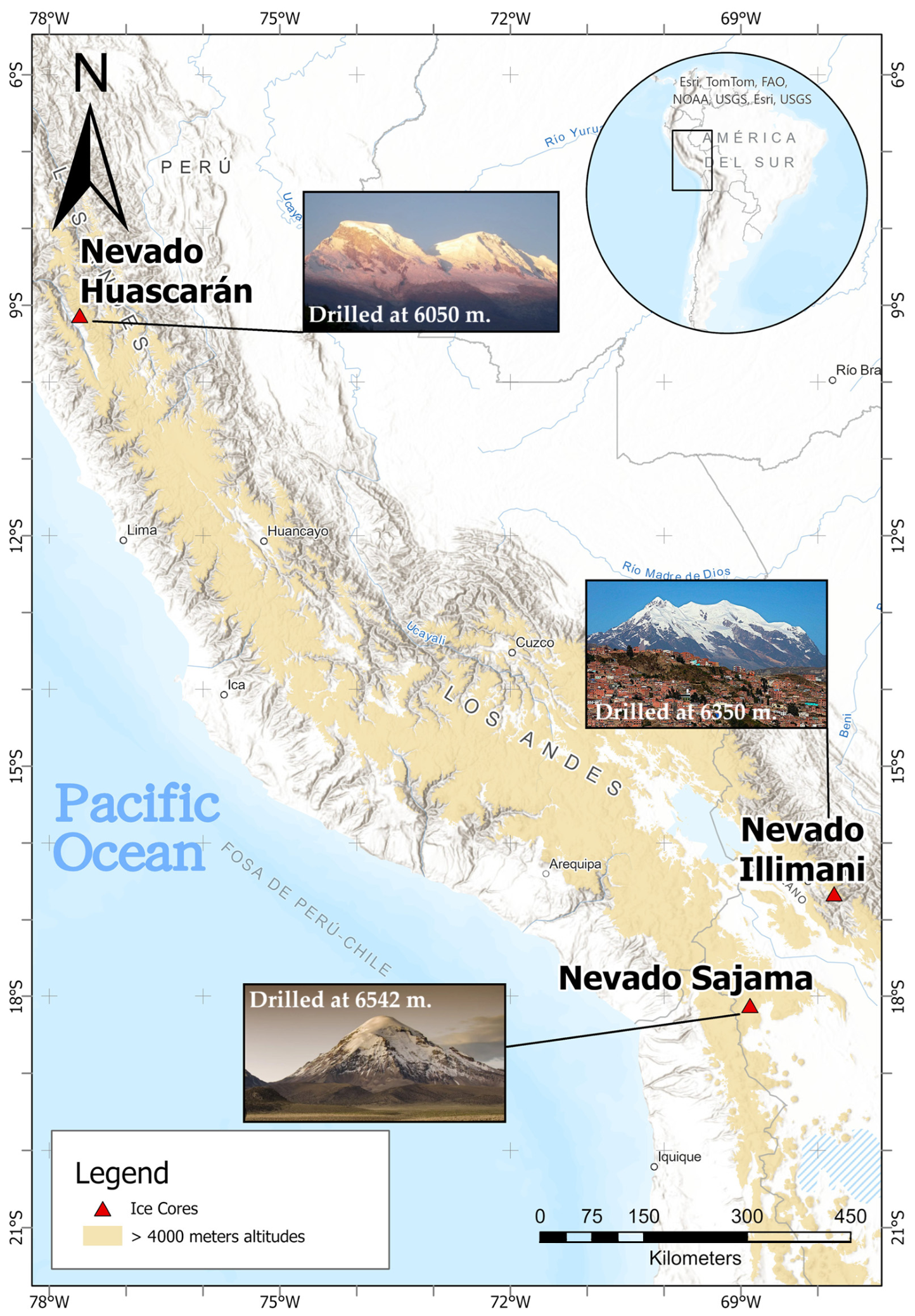
The analyzed ice cores are located in the Central Andes mountains (Figure 1) of Peru and Bolivia. This region extends from Huancabamba (Peru) at 5° S to the Colorado River basin in the north of the province of Neuquén (Argentina), at 30° S. This section of the Andes contains some of the highest peaks in the range, including the Nevado Huascarán (the 5th highest peak in the Andes with 6757 m) and Nevado Sajama (15th highest peak in the Andes with 6542 m).
Figure 1.
Geographic location of the analyzed ice cores. Coordinates in the main text.
In this context, some ice cores were drilled between 1995 and 2003 in glacial ice caps. The Huascarán ice core was drilled in the Cordillera Blanca of Peru (9°16′9.46″ S, 77°29′50.64″ W; 6050 m above sea level), while the Sajama core was drilled in the Central Volcanic Zone of Bolivia (18°6′39.96″ S, 68°53′0.24″ W; 6542 m above sea level). The information is complemented by the stable hydrogen isotope series from the Illimani core that was drilled in the Cordillera Real of Bolivia (16°37′51.24″ S, 67°47′29.40″ W; 6350 m a.s.l.). These records are representative of past temperatures at high altitudes of the Central Andes, as they were all drilled at altitudes above 6000 m a.s.l. as oxygen and deuterium signals in summit ice core records are always related to temperatures more than changes in precipitation [25].
The climate of the Central Andes, as a high mountain system, is strongly influenced by the altitude modification of temperature, its tropical position and the Andean barrier to moisture fluxes from the Amazon basin and Pacific Ocean. Slope orientation and proximity to the Pacific Ocean exert a key influence on aridity [26]. Solid or liquid precipitation is mainly related to changes in latitude of the Intertropical Convergence Zone (ITCZ) [27] and to El Niño-Southern Oscillation pattern [28]. Above 5500–6000 m, lower accumulated annual precipitation and permanent snow cover allow lower temperatures than would be expected based solely on altitudinal lapse rates [26].
Throughout the Pleistocene and Holocene periods, the described climatic patterns and forcings have exhibited relative variability. Evidence indicates that, in the Central Andes of Peru and Bolivia, the last glacial advance or Last Glacial Maximum occurred at around 34 ka, with the retreat period beginning around 21 ka [29]. Rather than a single existing LGM period across the entire Central Andes mountains, many authors have considered the possibility of having local maxima for different sub-regions (e.g., Bromley et al. [30], Blard et al. [31]). These local-LGM phases were also driven by multiple factors such as a global cooling of 3–6 °C [32] or a further southward shift of the Intertropical Convergence Zone [33].
2. Materials and Methods
The data from the Huascarán and Sajama cores were extracted from the National Oceanic and Atmospheric Administration (NOAA, Washington, DC, USA) repository. These data correspond to the work of Thompson et al. [12,13]. The Illimani data were taken from Ramírez et al. [14].
The three ice cores span from 25,000 to 18,000 years BP, covering the end of the Pleistocene and the whole Holocene (Table 1). In this work, a time interval from 7000 years to the present was selected in order to consider a relatively understudied interval, the Holocene epoch.
Table 1.
Characteristics of the three ice cores analyzed.
The number of samples used in each of the records were 82 samples (of a total of 252) in the case of Nevado Sajama ice core, 82 samples (of a total of 193) for Nevado Huascarán and 143 samples (of a total of 213) in the Nevado Illimani ice core.
2.1. Stable Isotopes in Ice as Indicators of Palaeotemperatures
The ratio of stable oxygen isotopes δ18O and hydrogen δD in glacial ice reflects the isotopic composition of precipitation over the duration of snowfall and, from this, palaeotemperatures can be estimated (e.g., Martín-Chivelet and Muñoz-García [34], or McDermott [35]). The study of δ18O (and δD) stratigraphy allowed the analysis of relative temperature variations in the intervals considered.
An important consideration is the resolution of the age models on which the time series of these cores are based. Ice exhibits plastic behavior, and layer counting (annual stratigraphy), whether visual or geochemical, can only be applied to the most recent levels (the last few centuries). Furthermore, 14C dating of organic remains trapped in the ice, and correlation with other better-dated records allowed for a more refined dating of the late Pleistocene levels. However, most of the Holocene ice records (between 3.3 and 9.7 ka in the case of Sajama and essentially the entire Holocene record in the case of Huascarán) were dated using a mathematical age model. In the case of Illimani, the published age model was based on the correlation of major events (such as the Younger Dryas, 11.7 ka) with the Sajama record [14]. The minimum error estimated for all age models was ±200 years. This significant limitation must be considered in intercomparisons between the series from the three records.
While the level of uncertainty of ±200 years had a limited impact on millennial-scale periodicities, such as those close to the characteristic periodicity of Bond cycles, it may partially blur or shift shorter-period signals on the order of a few hundred years. For this reason, correlations involving centennial-scale cycles and their alignment with solar or oceanic forcings were interpreted cautiously, whereas the consistency of longer-period variability between independent records supports the robustness of the millennial-scale climate signals identified in this study.
As the three revisited ice cores were drilled at high altitudes (above 6000 m) the palaeotemperatures could be representative of high-elevation Andean conditions. To the authors’ knowledge, no other proxies or cores were found at these altitudes in the Central Andes region. High altitude ice cores are representative of glacier feeding areas, which exhibit distinct climatic characteristics due to permanent snow, and summit climate dynamics. As these ice cores were drilled in those glacier feeding areas, the palaeoprecipitation and palaeotemperature signals can be preserved with minimal post-depositional alteration [36].
2.2. Statistical Preprocessing
To simplify the visual and statistical comparison of the paleoclimate series, the procedure involved removing long-term trends (“detrending”) superimposed on variability on a centennial or millennial scale. To achieve this, a linear fit was used in the case of Sajama and a second-order polynomial fit in Huascarán.
The type of detrending applied to each of the records was selected by measuring the similarity to a linear trend or to a first- or second-order polynomial trend. Similarity is assessed using the software RStudio (version 4.5.2.), from the astsa package [37] for the polynomial exploration and the “lm” function that is included in base R. According to the similarity of each record, the detrending was performed in the PAST software [38], a statistical application usually used in palaeoclimatology in order to pre-process data records and to support data interpretation [39,40].
2.3. Palaeoclimatic Periodicities
A spectral analysis of the Illimani, Huascarán and Sajama time series was also performed to identify possible periodic elements in climate variability. For this purpose, the PAST software [38] was again used, which works with the Lomb periodogram algorithm [22], which allows the calculation of spectral diagrams from time series with non-equidistant values. The aim was to process the detrended data series in order to find possible cycles that could be hidden to the unaided eye.
Spectral analysis techniques represent an optimal statistical approach for decomposing and identifying underlying periodicities in data series [22]. These techniques have been successfully applied in the field of Earth sciences and, more generally, in research related to solar periodicity [41,42] or modern climatology like El Niño-Southern Oscillation patterns (ENSO; [43]) or Bolivian Altiplano precipitation [44]. It has also been used for addressing the periodicities behind the global glacier retreat during the last deglaciation [45].
The formula on which the Lomb–Scargle periodogram is based is shown in Equations (1) and (2).
where is defined by:
The values m and s2 were estimates of the mean and variance of the data, {z(t1), z(t2), …, z(tN)}, and wj is the angular frequency (radians per unit time). The variable ƒj = wj/(2π) was the frequency in cycles per unit time of the sample. The parameter τ made the estimator of Equation (1), I(wj), independent of time. This estimator I(wj) is the Lomb–Scargle periodogram for the frequency wj.
The analysis also showed a minimum significance or spectral power for each period of the data series, which is indicative of the frequency with which each of the periodicities occurs and is referenced as a p-value. The PAST software estimated significance using randomization tests (Monte Carlo/permutation test), an empirical test, not theoretical. The Monte Carlo approach was based on the analyzed data series, while the software was being requested to calculate a power spectrum through P(f). The spectrum was given when synthetic-random series were created. The minimum significance, expressed as spectral power, was above 3.1.
The periodicities found were interpreted as cycles of maximum and minimum temperatures. The peaks were correlated between each other and compared with climate forcings or climate patterns.
Unlike classical Fourier-based methods that require evenly sampled data or interpolation, the Lomb–Scargle spectral analysis was selected because it is particularly well suited for paleoclimate time series derived from ice core records. These records are commonly unevenly spaced due to variable accumulation rates, layer thinning with depth, and age-model uncertainties.
2.4. Palaeoclimatic Patterns and Forcings
Both spectral analysis and visual correlation were compared with palaeoclimate drivers’ data records. These drivers or forcing series were obtained from literature research and NOAA. The climate forcings selected for comparisons were:
- Glaciomarine sediments: indicative of freshwater entrances in the North Atlantic and also referred to as Bond cycles [46].
- Solar irradiation: Steinhilber et al. [47] created a global estimation of the solar irradiation obtained from the geomagnetic field with 10Be analysis.
- Holocene volcanic activity: data obtained regarding to Volcanic Explosivity Index (VEI) values of 6 and 7 and located in low latitudes (<15°). These data were obtained from the Smithsonian volcanic institution.
All the comparisons of climatic drivers were used during visual correlation, but glaciomarine sediments were used also for periodicities’ comparisons.
Main cold and warm episodes were identified as abrupt changes of 18O or deuterium, understanding “abrupt” as a change of at least twice the mean value of the three previous samples. For clarity, the identified cold and warm episodes were numbered sequentially from the oldest (Episode VI) to the most recent (Episode I) in Table 2 and Table 3. Cold and warm phases were described separately but presented in chronological order, allowing direct comparison between the three ice core records.
Table 2.
Warm episodes identified according to each of the Andean data series. Episode denomination is indicated in the header.
Table 3.
Cold episodes identified according to each of the Andean data series. Episode denomination is indicated in the header.
3. Results
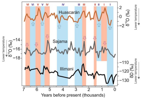
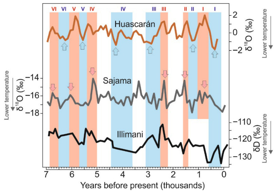
The Sajama and Huascarán δ18O series (Figure 2), which also includes the δD record from the Illimani ice core, showed significant variability during the mid and late Holocene. The heaviest δ18O values corresponded to higher temperatures and vice versa, allowing the identification of alternating centennial-scale warming and cooling intervals in each series (Figure 2), as well as a series of episodes of relative minimum and maximum temperatures. A comparative analysis of the series allowed the detection of patterns of common variability.
Figure 2.
Stable isotopes (δ18O and δD) data series from the Illimani, Sajama and Huascarán ice cores. Blue arrows indicate main cold episodes, while red arrows indicate maximum temperature episodes. Red and blue columns express correlated events.
3.1. Overview of Isotope Variability
The δ18O and δD records from the Sajama, Huascarán, and Illimani ice cores exhibit multi-centennial to millennial-scale variability throughout the last 7 ka. Periods of relatively enriched isotope values generally correspond to intervals interpreted as warm phases, while depleted values are associated with colder intervals. Although the three series show broadly similar long-term patterns, their degree of coherence varies. Sajama and Huascarán display clearer and more internally consistent structures, whereas Illimani shows greater dispersion and weaker alignment, likely reflecting differences in resolution and the limitations inherent to the digitized version of the dataset.
3.2. Correlation of Ice Core Records
The δ18O values range from 2 to −2 in Huascarán ice cap, whereas those from Sajama range from −14 to −18. In the case of Nevado Illimani, the δDeuterium values range from −110 to −130. All the three records showed a relative variability during the 7 ka analyzed.
A tentative correlation of the local climatic maxima and minima was therefore established, assuming that the ice cores in the study area should have been essentially contemporaneous. Therefore, the small lags between them were attributed to the age-model uncertainties.
A total of six climatic maxima and six minima common in at least Nevado Sajama and Nevado Huascarán were identified (Figure 2, Table 2 and Table 3). Climate variability during the mid and late Holocene was marked by recurrent cold and warm episodes in both regions, demonstrating that short-term variability was established during this interval.
Warm episodes are located approximately at 6.8–6.4 ka, 6.0–5.6 ka, 5.4–5.0 ka, 2.5–2.2 ka, 1.6–1.4 ka, and 0.7–0.4 ka, showing regional consistency although with slight variations between cores. Cold episodes appear near 6.6–5.9 ka, 5.7–5.2 ka, 4.0–3.6 ka, 2.7–2.6 ka, ~1.4–1.2 ka, and 0.3–0.1 ka.
Regarding the warming events, all the six identified episodes were contemporaneous for Nevado Huascarán, Nevado Sajama and Nevado Illimani. Usually, these events were alternated in sequence, except between ~4.2 and ~1.2 ka, where two cold episodes are present (~4.2–2.9 ka) followed by warm episodes (~2.2–1.9 ka). There was only a period between 5 and 2.5 ka that showed a relative stability or “deep valley” with no warm periods.
Additionally, cold events showed a broader range of values under the adopted event-definition criteria. Some similarities were found between cold events’ time ranges, but at least for the 5.9 ka and 4.0 ka event, the time frame of the duration could be even greater. In the case of Nevado Illimani, this ice core did not exhibit strong synchronicity with the rest of the records, even lacking one of the episodes, such as the 1.4–1.2 ka (Episode II). The three analyzed records exhibited a similar decreasing trend.
3.3. Spectral Analysis
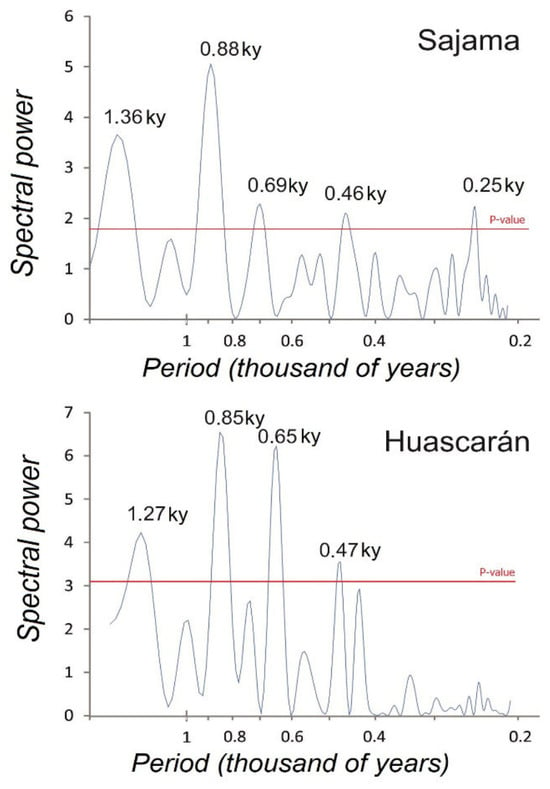
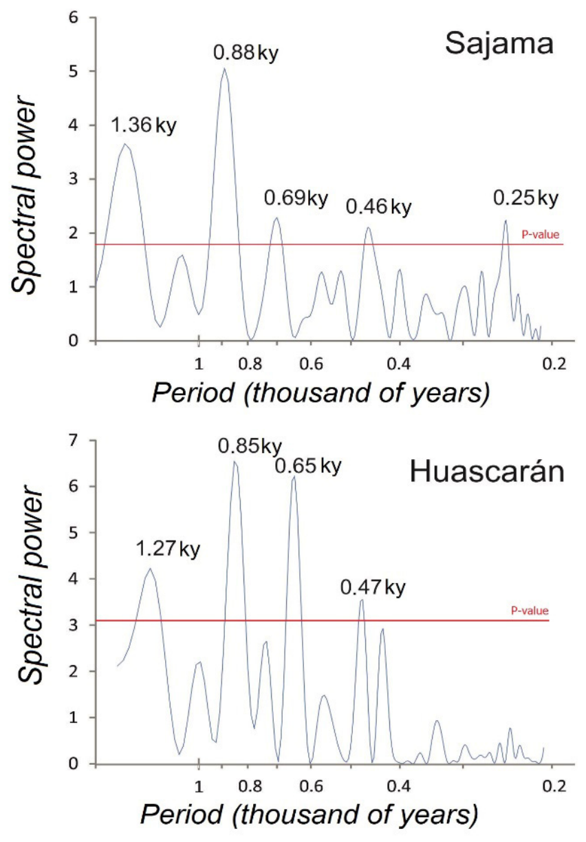
The results of the spectral analysis of the two records with the highest number of samples, represented in the spectral diagrams (Figure 3), showed notable similarities. Spectral maxima were detected around 1.3, 0.87, 0.67, 0.46, and 0.25 kiloyears, although the latter presents a very low level of significance in Huascarán. Therefore, identified cycles represent millennial-scale variability (1.3 and 0.87 ka) and centennial scales (0.67, 0.46 and 0.25 ka).
Figure 3.
Spectral diagrams of the oxygen isotopes data series derived from Andean ice cores. The most significant spectral peaks are indicated in thousands of years.
Then, the most clearly defined peaks occur in the millennial band, particularly around 1.3 ka, where both records exhibit a well-developed spectral signal. Additional peaks are observed at sub-millennial frequencies, although their amplitudes vary slightly between the two datasets.
The minimum significance was above 3.1 for the Nevado Huascarán and 1.85 for the Nevado Sajama data records. Nevado Illimani records returned multiple errors during the tests as all the periodicities were below the p-value (or did not exceed the significance threshold), which was stipulated as value 2.6.
Unfortunately, deuterium levels from the Nevado Illimani record were not accessible on the bibliography or any record website. Even so, a digitization procedure by picking points was applied in order to transfer the data of the graphic shown in the Ramírez et al. [14] paper into an Excel® dataset. Digitization was performed with WebPlotDigitize® software, version 4. The results of the spectral analysis showed no valid periodicities as all of them were below significance or p-values. Therefore, Illimani is not used to support any spectral interpretations, and periodicity-based conclusions draw exclusively on Sajama and Huascarán.
4. Discussion
On the one hand, the identification of essentially contemporaneous climate minima and maxima (within the margins of error) in the three ice cores analyzed were essential to understand the common climate patterns in Central Andes summits. On the other hand, the significant coincidences in cyclicity revealed by the spectral analysis highlighted the supraregional nature of climate changes during the mid and late Holocene.
To discuss the possible origin of these climate changes, the Andean records were compared with well-established climate-forcing and climate-pattern time series. Specifically, the comparisons included the total solar irradiance series [47], volcanic activity periods and relative activity series of the thermohaline circulation in the North Atlantic (records of glacioderived deposits in the North Atlantic, [46]).
It is important to note that the identified relationships are based on qualitative comparisons between proxy records and external forcing series. Although consistent patterns are observed, and statistical methods, such as spectral analysis, are applied, further research is needed, limiting the ability to establish robust causal links. Therefore, the proposed mechanisms should be interpreted as plausible hypotheses rather than definitive conclusions.
Although the present study relies on correlation analyses between Andean ice core records and large-scale climate forcings, several physically based mechanisms are proposed to explain how solar variability and changes in North Atlantic Ocean circulation may influence temperature variability in the tropical Andes.
4.1. Possible Regional Synchronicity
The broadly contemporaneous cold and warm phases identified across the three ice cores raise the possibility that Central Andean climate fluctuations during the mid and late Holocene were regionally coherent rather than locally confined. This, however, remains a hypothesis.
The periodicities near 1.3 ka detected in the Sajama and Huascarán spectral analyses are broadly consistent with millennial-scale variability documented elsewhere, but their attribution to mechanisms such as Bond-like cycles should be treated as tentative. The correlations drawn with external forcings rest partly on visual alignment rather than formal statistical testing and must, therefore, be understood as possible associations rather than demonstrated causal links. Such relationships likely reflect a combination of climatic processes and should be assessed in light of the chronological uncertainties inherent to both records.
Although no statistically significant periodicities were identified in the Illimani series, the temporal alignment of major isotopic excursions with those observed in Sajama and Huascarán suggests that it retains a coherent signal at the centennial-to-millennial scale. Illimani provides an independent line of evidence supporting the timing of major climatic events identified in the other cores.
4.2. Warm and Cold Episodes
Nevado Huascarán and Nevado Illimani have been shown to exhibit similar climate variability during the Pleistocene and Holocene periods. Ramirez et al. [14] described the paleoclimate variations as similar, but differing from Nevado Sajama, which was possibly influenced by local conditions such as increases in moisture and precipitation. In contrast, this research has found a good correlation for the mid–late Holocene period, suggesting that local conditions were not the primary driver during the mid and late Holocene in Nevado Sajama as aridity was gaining presence. On the contrary, general South American atmospheric dynamics and teleconnections with interhemispheric processes may be behind Holocene climate variability.
At a local scale it is also possible to observe some coincidences between the cold and warm episodes identified in this study and other research. A possible strong synchronicity of all the three ice cores records here analyzed was observed, with six common cold and warm episodes. These records also exhibited a similar decreasing trend, indicating that even though the Holocene is a warm period there was a progressive cooling before human influence.
Some of the identified episodes, such as the cold episode V, match cold conditions as marked by Weng et al. [48] in palynological analysis from La Compuerta lake at 3950 m elevation, and located at 230 km north-west to the Huascaran glacier. This record also indicated conditions coincident with warm episode IV at 5.0 ka.
The paleoclimatic research in Nussloch, Germany, [49] also identified a 4.2 ka potential anomaly that could match the cold episode IV (4.0–3.9 ka) registered in the Central Andes ice cores revisited here.
The cold episode IV matches perfectly, as well, with glacier advances in the same study area. Cordillera Blanca may have experienced glacier readvances at 4 ka while the Nevado Sajama may have advances around the 4.4 ka [12]. The advances support the cold episode IV, as some other episodes could be missing in the glacier record after geomorphological eroding of longest advances or during the Little Ice Age.
Glacier advances could not exactly match warm or cold episodes if temperature or precipitation changes are gradual rather than abrupt. Glaciers respond to climate forcing with inherent time lags and integrate temperature and precipitation changes over their response times. Therefore, gradual or short-lived climatic variations may produce delayed, muted, or even no discernible geomorphological response in the glacier record [50,51].
Dry conditions [52] and a lack of glacier readvances are also coincident with a halt in climate variability between the ~1.5 ka cold episode II and the warm episode I during 0.4–0.7 ka. The cold episode I was coincident with the regional expression of the Little Ice Age described for the Central Andes [53,54].
4.3. Bond Cycles and Their Relationship with Andean Climatology
The AMOC (Atlantic Meridional Overturning Circulation or thermohaline current) velocity is closely related to the meltwater flux that is naturally introduced in the North Atlantic area through iceberg calving and terrestrial runoff [55]. These processes occur in cyclic “pulses” known as Heinrich Events, if the temporal scale ranges between 7 and 10 ka. or Dansgaard–Oeschger or Bond cycles if it occurs each 1.5 ka. While Dansgaard-Oeschger events are related to the Pleistocene period, Bond cycles are often referred to as Holocene phenomena [56].
It is known that changes in the velocity of the thermohaline current (or a possible shut-off) can modify the interhemispheric energy balance, resulting in short-term global temperature variations. Slowing periods in the AMOC are closely related to rapid climate changes in abrupt cooling detected for the North Atlantic, but also for some other interconnected regions [57].
As tropical Atlantic sea surface temperatures influence the large-scale atmospheric circulation, tropical eastern Pacific climate could be linked to AMOC [58]. Thermohaline circulation weakening is also a modulator of the Pacific El Niño pattern [59]. Many authors concluded a direct relationship between ENSO or the Central Andes present temperatures [60] and Holocene palaeotemperatures [61].
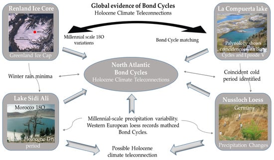
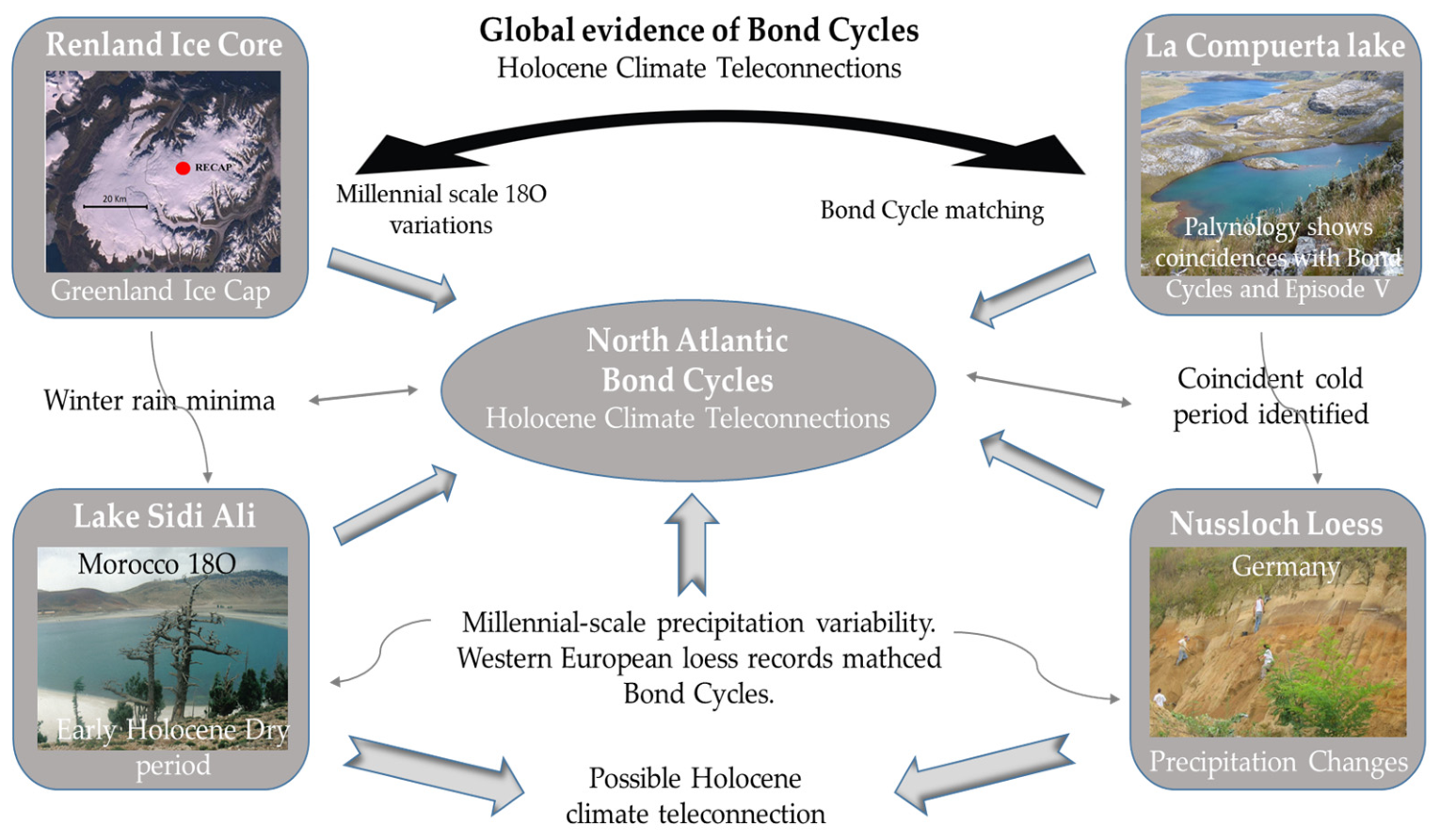
The previously mentioned Bond cycles have been identified in different records sampled worldwide (Figure 4), suggesting a possible Holocene teleconnection with the North Atlantic. The Renland ice core record (east central Greenland coast) showed climate variabilities in δ18O levels that were matched to a millennial-scale cycle in line with Bond cycles [62].
Figure 4.
Relationship between Bond cycles and oxygen isotopes records.
Zielhofer et al. [63] found a noticeable lack of winter rain in the western Mediterranean during the Early Holocene through δ18O records in Lake Sidi Ali (Morocco). The rainfall minima coincided with Bond events while the opposite situation was found for the Late Holocene.
Records of the western European loess cores in the previously mentioned Nussloch region (Germany) also matched North Atlantic variability, as they showed millennial scale changes in precipitation. This variability was linked to Bond cycles [49]. This could be an example of teleconnections between distant climate forcings.
Links between North Atlantic Bond cycles and Aegean Sea climate fluctuations (eastern Mediterranean) were also identified through spectral analysis of Ti/Al (Titanium/Aluminum) and Zr/Si (Zircon/Silica) records from a sediment core [64]. Among others, this research found a 1200-year periodicity, closely related to the variability identified here in the Central Andes.
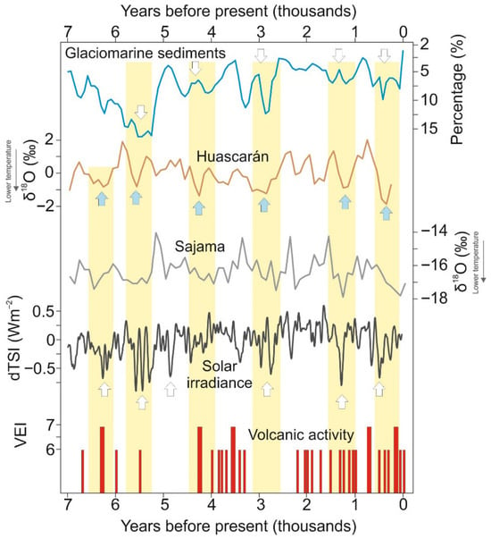
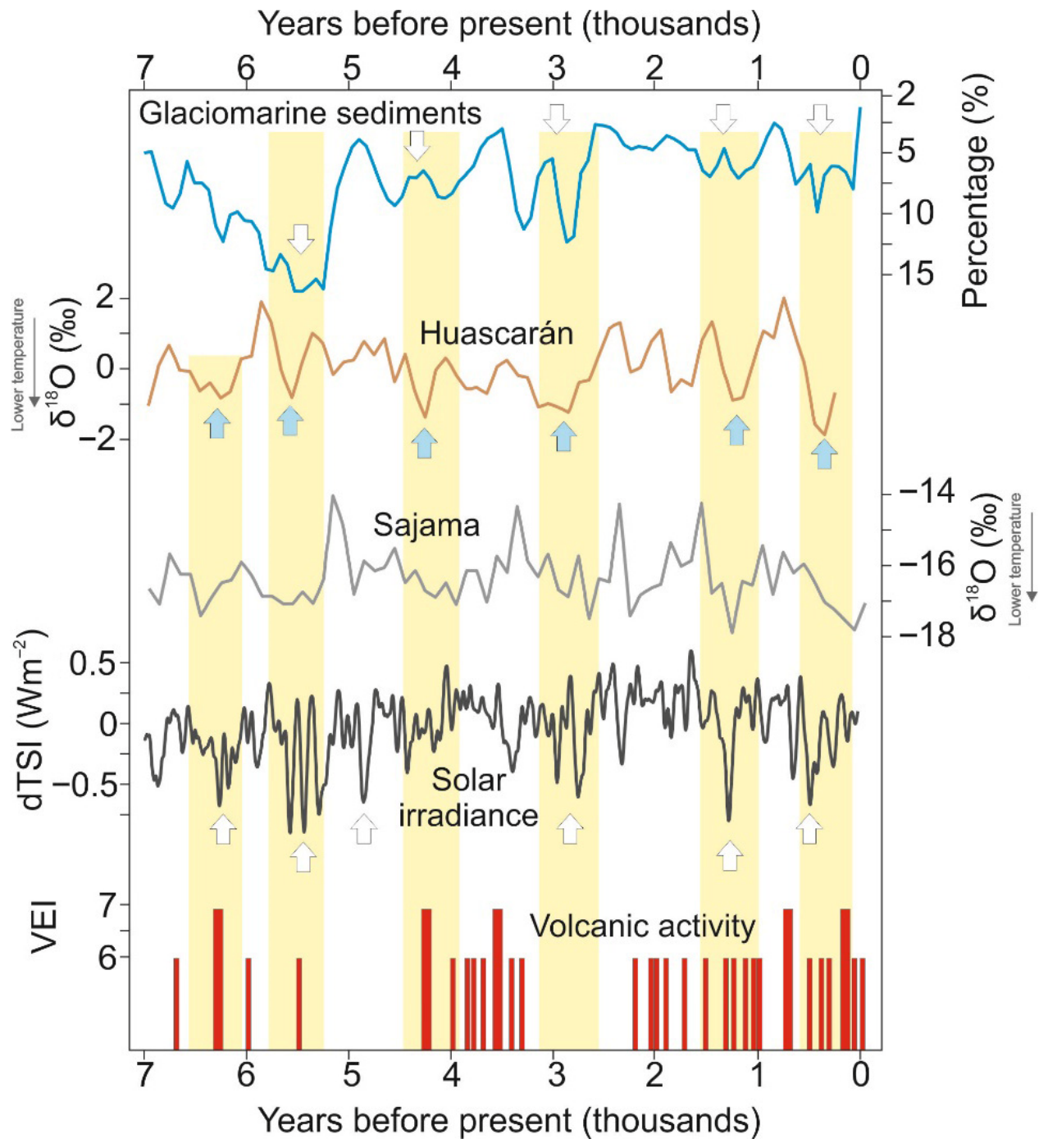
Knowing that the thermohaline current exerts an interhemispheric influence [57,65], possible teleconnections with the study area are expected. Glacial deposits derived from the North Atlantic showed the existence of five maxima, all of which correspond well with the Andean climatic minima identified in this study (Figure 5). The glacial deposits in the North Atlantic are direct evidence of the thermohaline circulation, and the good correlation of all the maxima in the glaciomarine record with 5 in 6 of the cold events in the three ice records is unlikely to be coincidental. This research could also provide additional statistical evidence through the similarity of periodicities, the similarity between periodicity cycles. Nevado Sajama and Nevado Huascarán both exhibit periodicities of approximately 1.3 ka. In parallel, the periodicities recognized in the spectral analysis could be interpreted as connected to the global climate cycles related to the AMOC as climate forcing. Specifically, the cycles defined by the longest periods (around 1.3 ka.) are close to the average length of Bond cycles, 1.5 ka. based on the recurrence of glacioderived deposits in the Atlantic and associated with changes in thermohaline circulation.
Figure 5.
Comparison of the stable isotopes data series from Sajama and Huascarán ice cores with glaciomarine deposits of the Northern Atlantic (values expressed as percentage of hematite grains; arrows indicate maxima corresponding to major iceberg discharge events in the Atlantic, Bond et al. [31]), with sun activity reconstruction (arrows indicating big solar minima; Steinhilber et al. [30]) and volcanic activity (Volcanic Explosivity Index > 6) data from Smithsonian Institution Archives [66]. Yellow columns expressing correlation.
As previously mentioned, the AMOC is a key climate forcing for its role in energy distribution between hemispheres. Spectral analysis points to a possible external control in the Huascarán and Sajama records, while the correlation analysis suggests that this influence may extend to all three ice cores. Variations in solar irradiance can modify large-scale atmospheric circulation and the meridional energy balance, leading to temperature changes in high-elevation tropical regions.
In parallel, variations in the strength of the Atlantic Meridional Overturning Circulation affect interhemispheric heat transport, influencing tropical Atlantic sea surface temperatures and atmospheric circulation patterns. Modeling and paleoclimate studies have shown that AMOC slowdowns can propagate to the tropical Pacific through atmospheric teleconnections, modulating ENSO-like variability (e.g., Timmermann et al., [58]). Since ENSO exerts a strong control on air temperature over the Central Andes, particularly at high elevations, these teleconnection pathways provide a physically consistent framework linking high-latitude forcings with the supraregional temperature variability observed in the Andean ice core records.
Beyond these teleconnections, the transmission of high-latitude forcings to the Central Andes is likely mediated by changes in the mean state of the tropical atmosphere, including shifts in the position and intensity of the Hadley circulation and the Intertropical Convergence Zone. Bond cycles may induce shifts in the ITCZ and Hadley circulation by modifying the hemispheric heat gradient [67,68]. Such circulation adjustments affect upper-tropospheric temperature gradients and lapse rates, which are particularly relevant for high-elevation regions where ice cores are drilled [69,70]. Climate modeling and paleoclimate evidence indicate that these atmospheric reorganizations can produce coherent temperature anomalies across tropical mountain regions without requiring abrupt local forcing, providing a plausible mechanism for the synchronous temperature variability recorded in the Nevado Sajama, Nevado Huascarán, and Nevado Illimani ice cores [71,72].
In this context, the aforementioned period of climatic stability between 5 and 2.5 ka or “deep valley”, coincides with ENSO events that were less frequent or weaker than at present between ~5000 and 3000 years ago [73,74]. It may be possible to establish a relationship between the weakening of Bond cycles and the lower frequency of ENSO events. The weakening of the AMOC could lead to a cooler tropical Pacific Ocean, strengthening the Walker circulation and resulting in weaker ocean–atmosphere coupling. This, in turn, leads to a 30% decrease in ENSO variability and a lower number of extreme events. This transmission mechanism was observed in climate models that predicted a weakening of the AMOC [75]. However, other models observed the opposite situation, where a weakening of the thermohaline would change the Pacific SST, weakening the trade winds and thus increasing the variability of ENSO events [76]. Thus, the state of the AMOC can be considered to modulate ENSO to some extent, but it does not control its phase.
Regarding the Little Ice Age (LIA) event in the Central Andes, this period (0.3–0.1 ka) is defined as an abrupt cooling by many authors [71], indicating that the climate drivers behind the onset of this event should therefore involve rapidly acting forcing. Given that the solar minima forcing is a somewhat gradual climate forcing, the LIA event could have been driven by volcanic eruptions, but also by other rapidly acting forcings, such as an AMOC slowdown.
The glaciomarine sediment record analyzed in this research showed a decrease also coincident with the onset and duration of the LIA event. A classic hypothesis proposed that a change in global thermohaline circulation accompanied the LIA.
However, Broecker [77] emphasized that this remained speculative and required more evidence. Recently, the possible influence of the AMOC circulation on the LIA event has also been addressed by some research as surface AMOC/subpolar gyre changes could have amplified both Medieval warmth and LIA cooling, at least for the North Atlantic sector [78], whereas other authors do not directly attribute the LIA to AMOC variability, but consider a freshwater input from the Labrador Current due to a thickening of the Arctic sea ice [79]. Further research is needed to assess the role of the AMOC in the Little Ice Age.
Some authors have questioned the actual existence of Bond cycles, suggesting that climate changes may result from multiple interacting causes rather than solely from meltwater forcing [80]. As these melting pulses could be the key triggering factor for the abrupt changes in the Early Holocene, some other changes for the Late Holocene could be caused by a combination of mechanisms such as volcanic patterns, orbital insolation or solar activity [81,82,83].
4.4. Comparison with Volcanic Activity
Regarding Holocene volcanic activity, a moderate correlation has been observed. The 4.0 ka cold event shows a reasonable temporal correspondence with the Cerro Blanco eruption in 4.3–4.2 ka [65] but also with a low activity of the AMOC as seen in the glacioderived sediments. Also, the 6.4–5.9 ka cold event could not be explained by the AMOC activity due to the high levels of glaciomarine sediments. On the contrary, the Kikai eruption at 6.4 ka and a deep solar minimum correlates with the drop in δ18O values in Sajama and Huascarán.
The 0.2 ka cold event, or the Little Ice Age event, could be somehow related to grand solar minima, as indicated globally by Owens et al. [84] and Wanner et al. [85]. As well, there is strong evidence that this event could be initiated and maintained by an increase in the volcanic activity based on several sulfur-rich eruptions (e.g., Samalas 1257 A.D., Kuwae 1452 A.D., Huaynaputina 1600 A.D. or Tambora 1815 A.D.; [86,87,88,89]).
Overall, the results highlighted coherent patterns between Andean climate variability and large-scale forcings; however, these relationships should be interpreted as hypotheses that require further quantitative testing.
4.5. Solar Activity and Its Relationship with Andean Climatology
In this research, shorter-period cycles of 0.69 and 0.25 ka could tentatively correspond to solar cycles of comparable duration [90,91].
Comparison of δ18O records from ice cores with forcing factor records (Figure 4) suggests a strong influence of solar activity on the three Central Andes ice cores. The major solar minima that mark the studied interval generally correspond well with episodes of minimum temperatures in the Central Andes. Solar irradiance is the main driver for climatic circulation on Earth [47] and the paleoclimatic influence of solar activity has been widely documented [92,93].
The Tropical Andes have been found to be very sensitive to even small changes in solar radiative forcing. Reduced solar activity in the Andes led to the Little Ice Age with a temperature decline of −3.2 °C (±1.4 °C) at least for the Venezuelan Andes [56,57]. Unfortunately, there is still a lack of high-resolution data at shorter timescales to indicate the solar influence on past temperatures, as existing records lack sufficient accuracy and resolution [94].
In the Laguna Comercocha of the Peruvian Andes, changes in solar activity have been linked to precipitation patterns through the modification of the South American Summer Monsoon intensity [95]. Therefore, either directly through reduced radiative forcing or indirectly through modifications of large-scale atmospheric circulation, solar forcing could be a key factor for the middle and late Holocene variability, as revealed in the three reviewed ice cores.
From all these findings, it can be deduced that the combined (and possibly interconnected) influence of solar activity and thermohaline circulation could exert a certain influence on climatic variations in the Southern Hemisphere, particularly in the Central Andes.
4.6. Modern Implications on Climate Variability
The millennial-scale climate variability identified in Central Andean ice core records provides long-term context for understanding the magnitude and drivers of the current phase of glacier retreat. In contrast to the Holocene cold and warm episodes discussed here—many of which were associated with gradual changes in solar forcing, ocean circulation, or episodic volcanic activity—the present warming is characterized by an unprecedented rate of temperature increase driven primarily by anthropogenic greenhouse gas emissions [96].
Recent research [21,97] emphasizes that while past glacier fluctuations were often linked to natural forcing mechanisms and regional hydroclimatic reorganizations, the current warming trajectory exceeds Holocene background variability in both speed and spatial coherence.
Current climate change differs from the mid and late Holocene variability as the rate of warming in recent decades has been accelerating [98]. In contrast, past climate changes appear to have been gradual, or, when rapid, the change could have occurred from millennial to centennial timescales [99,100].
From a forward-looking perspective, accelerated deglaciation under continued global warming may have implications not only for regional water resources but also for large-scale climate feedbacks. Sustained meltwater input from rapidly shrinking glaciers and ice masses could contribute to changes in ocean salinity and stratification, particularly if future warming leads to enhanced freshwater fluxes into key oceanic regions. Bond cycles during the Holocene are generally interpreted as internally driven, quasi-periodic responses of the climate system to freshwater perturbations and ocean circulation changes. The present-day magnitude and forcing context of meltwater release could favor a slowdown in the AMOC circulation. This scenario is not merely theoretical and has been discussed in recent studies.
Although many researchers indicate that the AMOC monitoring period is still too short to robustly detect an anthropogenic signal (as it began in 2004 [101]), new research has detected a possible 15% weakening of the thermohaline circulation since the mid-20th century [102]. The AMOC could be weaker today than at any other period in the last millennium, showing a rapid decline since the 20th century [103].
Nevertheless, the paleoclimatic evidence reviewed in this study highlights the sensitivity of the climate system to cryosphere–ocean interactions, suggesting that continued glacier loss could act as a modulating factor on future ocean circulation variability that may have no direct analogue in the Holocene, due to the increasing and constant introduction of meltwater in the ocean. The current situation is unlikely to be comparable to Bond cycles, given that these events were gradual and made from different periodic pulses of meltwater.
4.7. Shortcomings and Future Work
A series of shortcomings must be taken into consideration. Working with ancient climate records, even if complete, faces several challenges. First, the uncertainty of dating each of the ice layers could be within an error of ±200 years. This introduces a range of estimated ages that could affect the correlation between events at shorter timescales and should be considered when addressing this research.
Secondly, δ18O and δD estimations may reflect both temperature and precipitation variability. When precipitation remains relatively stable over time, temperature reconstructions are generally more reliable, and temperatures can be more reliable. As Nevado Sajama and Illimani were relatively arid regions during the Holocene, the uncertainty could be low. Nevado Huascarán may have experienced greater precipitation variability. However, temperatures composed the main variability during the mid and late Holocene.
Future work should revisit high-mountain Holocene records worldwide to assess the extent of Bond-cycle influence. Particular attention will be given to South America and Central Andes, as climate patterns remain relatively consistent. Identifying teleconnections between different hemispheric climate systems remains a key research objective. Assessing other palaeoclimate proxies, such as paleolake sediments, paleolake levels or cave speleothems should also be prioritized.
In future research, the AMOC weakening and its ENSO relationship will be addressed, aiming to determine whether Bond cycles may have influenced the ENSO variability during past Holocene periods. However, this analysis remains challenging, as El Niño events and Bond cycles do not occur on the same temporal scale.
Future research should focus on refining age models and increasing temporal resolution through additional high-altitude ice core drilling and multi-proxy approaches, as well as integrating these paleoclimate records with climate model simulations. Coupling proxy data with Holocene and future climate simulations would help to better quantify the mechanisms linking solar variability, ocean circulation, and tropical Andean temperature changes, and to assess how these natural modes of variability may interact with ongoing anthropogenic warming.
5. Conclusions
The results of this study provide valuable insights into long-term climate variability affecting high-elevation tropical regions, where instrumental records are scarce.
The main cold and warm episodes in the climate evolution of the Central Andes over the last seven millennia (mid to late Holocene) have been identified using available data from glacial ice cores collected in the area over the past few decades. The temporal resolution achieved in this study is unprecedented in the Holocene palaeoclimatology of the region. Therefore, spectral analysis techniques have been shown to be a powerful tool for understanding the relationship between climate forcings and palaeoclimatic variables.
A review of stable isotopes from ice core records from Nevado Huascarán (Peru), Nevado Sajama (Bolivia) and Nevado Illimani (Bolivia) showed a possible high degree of climatic synchronicity for the whole considered period (last 7 ka). Shared periodicities are most clearly expressed in the Sajama and Huascarán records, though the available evidence tentatively extends this pattern to all three ice cores. As in many other regions, late and middle Holocene variability of the Central Andes may be related to multiple direct and indirect forcings rather than a single driver.
After spectral analysis, periodicities of 1300 years in the palaeotemperatures have been identified. Shorter periodicities of 0.87, 0.69, 0.46, and 0.25 ka were also detected. The longest periodicity identified, 1.3 ka, suggests that Bond-cycle events may influence palaeotemperatures in the Central Andes, while shorter cycles such as 0.69 and 0.25 ka may correspond to solar activity. Mechanistically, high-latitude climate changes may influence the study area through modifications in the interhemispheric energy balance, shifts in the Hadley circulation, and latitudinal shifts of the Intertropical Convergence Zone.
Correlation analysis conducted on the ice-core records also showed the relationship between minimum temperature episodes and minima in solar activity. Also, warm and cold episodes have been identified as contemporaneous with nearby regions, including other parts of the Andes (also in the Central Andes).
Overall, the climate variability is interpreted as related to major changes in volcanic and solar activity during the Holocene, as well as long-term variations in thermohaline circulation (Bond cycles).
Author Contributions
Conceptualization, N.B.L.; Data curation, A.F.-S. and E.P.-C.; Formal analysis, A.F.-S.; Investigation, A.F.-S. and W.L.N.-C.; Methodology, A.F.-S. and J.A.Á.A.; Project administration, H.V.N.; Resources, D.Á.M.P.; Software, A.F.-S. and J.A.Á.A.; Supervision, W.L.N.-C., H.V.N. and D.Á.M.P.; Validation, J.A.Á.A.; Visualization, N.B.L. and W.L.N.-C.; Writing—original draft, A.F.-S.; Writing—review and editing, J.A.Á.A., N.B.L., W.L.N.-C., H.V.N. and D.Á.M.P. All authors have read and agreed to the published version of the manuscript.
Funding
This research received no external funding.
Institutional Review Board Statement
Not applicable.
Informed Consent Statement
Not applicable.
Data Availability Statement
Links to publicly archived datasets analyzed https://www.ncei.noaa.gov/access/paleo-search/ (accessed on 12 January 2024).
Acknowledgments
Authors want to thank the editorial board and anonymous reviewers for their appreciated comments. The team would also like to thank Korean Friendship Association for the precious support while researching.
Conflicts of Interest
Author Néstor Bernal López was employed by the company Tragsatec. The remaining authors declare that the research was conducted in the absence of any commercial or financial relationships that could be construed as a potential conflict of interest.
Abbreviations
The following abbreviations are used in this manuscript:
| ITCZ | Inter Tropical Convergence Zone |
| ENSO | El Niño Southern Oscillation |
| N. | Nevado |
| BP | Before Present |
| Ka | Kiloanni (one thousand years) |
References
- Azoulay, A. Message from Ms Audrey Azoulay, Director-General of UNESCO, on the Occasion of World Day for Glaciers and World Water Day, 21 and 22 March 2025. UNESCO Online, 22 March 2025. Available online: https://unesdoc.unesco.org/ark:/48223/pf0000393199 (accessed on 20 April 2025).
- Caro, A.; Condom, T.; Rabatel, A.; Champollion, N.; García, N.; Saavedra, F. Hydrological Response of Andean Catchments to Recent Glacier Mass Loss. Cryosphere 2024, 18, 2487–2507. [Google Scholar] [CrossRef] [Scilit]
- Grosjean, M.; Santoro, C.M.; Thompson, L.G.; Núñez, L.; Standen, V.G. Mid-Holocene climate and culture change in the South Central Andes. In Climate Change and Cultural Dynamics; Elsevier: Amsterdam, The Netherlands, 2007; pp. 51–115. [Google Scholar] [CrossRef] [Scilit]
- Guédron, S.; Delaere, C.; Fritz, S.C.; Tolu, J.; Sabatier, P.; Devel, A.-L.; Heredia, C.; Vérin, C.; Alves, E.Q.; Baker, P.A. Holocene variations in Lake Titicaca water level and their implications for sociopolitical developments in the central Andes. Proc. Natl. Acad. Sci. USA 2023, 120, e2215882120. [Google Scholar] [CrossRef] [Scilit]
- Orellana, H.; Latorre, C.; García, J.-L.; Lambert, F. Spatial analysis of paleoclimate variations based on proxy records in the south-central Andes (18°–35° S) from 32 to 4 ka. Quat. Sci. Rev. 2023, 313, 108174. [Google Scholar] [CrossRef] [Scilit]
- Nunnery, J.A.; Fritz, S.C.; Baker, P.A.; Salenbien, W. Lake-level variability in Salar de Coipasa, Bolivia during the past ~40,000 yr. Quat. Res. 2019, 91, 881–891. [Google Scholar] [CrossRef] [Scilit]
- Sae-Lim, J.N.; Konecky, B.L.; Hutchings, J.A.; Michelutti, N.; Grooms, C.; Vuille, M.; Castañeda, I.S.; Smol, J.P. Biomarker evidence for arid intervals during the past ~1,800 years in the central Andean highlands. Earth Planet. Sci. Lett. 2025, 662, 119407. [Google Scholar] [CrossRef] [Scilit]
- Jouzel, J.; Masson-Delmotte, V. Deep ice cores: The need for going back in time. Quat. Sci. Rev. 2010, 29, 3683–3689. [Google Scholar] [CrossRef] [Scilit]
- Eichler, A.; Gramlich, G.; Kellerhals, T.; Tobler, L.; Rehren, T.; Schwikowski, M. Ice-core evidence of earliest extensive copper metallurgy in the Andes 2700 years ago. Sci. Rep. 2017, 7, 41855. [Google Scholar] [CrossRef] [Scilit] [PubMed]
- Jouzel, J.; Alley, R.B.; Cuffey, K.M.; Dansgaard, W.; Grootes, P.; Hoffmann, G.; Johnsen, S.J.; Koster, R.D.; Peel, D.; Shuman, C.A.; et al. Validity of the temperature reconstruction from water isotopes in ice cores. J. Geophys. Res. 1997, 102, 26471–26487. [Google Scholar] [CrossRef] [Scilit]
- Johnsen, S.J.; Dahl-Jensen, D.; Gundestrup, N.; Steffensen, J.P.; Clausen, H.B.; Miller, H.; Masson-Delmotte, V.; Sveinbjörnsdottir, A.E.; White, J. Oxygen isotope and palaeotemperature records from six Greenland ice-core stations: Camp Century, Dye-3, GRIP, GISP2, Renland and NorthGRIP. J. Quat. Sci. 2001, 16, 299–307. [Google Scholar] [CrossRef] [Scilit]
- Thompson, L.G.; Mosley-Thompson, E.; Davis, M.E.; Lin, P.N.; Henderson, K.A.; Cole-Dai, J.; Bolzan, J.F.; Liu, K.B. Late Glacial Stage and Holocene Tropical Ice Core Records from Huascarán, Peru. Science 1995, 269, 46–50. [Google Scholar] [CrossRef] [Scilit]
- Thompson, L.G.; Davis, M.E.; Mosley-Thompson, E.; Sowers, T.A.; Henderson, K.A.; Zagorodnov, V.S.; Lin, P.-N.; Mikhalenko, V.N.; Campen, R.K.; Bolzan, J.F.; et al. A 25,000 Year Tropical Climate history from Bolivian Ice Cores. Science 1998, 282, 1858–1864. [Google Scholar] [CrossRef] [Scilit] [PubMed]
- Ramirez, E.; Hoffmann, G.; Taupin, J.D.; Francou, B.; Ribstein, P.; Caillon, N.; Ferron, F.A.; Landais, A.; Petit, J.R.; Pouyaud, B.; et al. A new Andean deep ice core from Nevado Illimani (6350 m), Bolivia. Earth Planet. Sci. Lett. 2003, 212, 337–350. [Google Scholar] [CrossRef] [Scilit]
- Eichler, A.; Gramlich, G.; Kellerhals, T.; Tobler, L.; Schwikowski, M. Pb pollution from leaded gasoline in South America in the context of a 2000-year metallurgical history. Sci. Adv. 2015, 1, e1400196. [Google Scholar] [CrossRef] [Scilit]
- Wang, N. Evidence for cold events in the early Holocene from the Guliya ice core, Tibetan Plateau, China. Chin. Sci. Bull. 2002, 47, 1422. [Google Scholar] [CrossRef] [Scilit]
- Parker, S.E.; Harrison, S.P. The timing, duration and magnitude of the 8.2 ka event in global speleothem records. Sci. Rep. 2022, 12, 10542. [Google Scholar] [CrossRef] [Scilit]
- Alley, R.B.; Mayewski, P.A.; Sowers, T.; Stuiver, M.; Taylor, K.C.; Clark, P.U. Holocene climatic instability: A prominent, widespread event 8200 yr ago. Geol 1997, 25, 483–486. [Google Scholar] [CrossRef] [Scilit]
- Toohey, J.L.; Murphy, M.S.; Chirinos Ogata, P.; Stagg, S.G.; Garcia-Putnam, A. A monumental stone plaza at 4750 B.P. in the Cajamarca Valley of Peru. Sci. Adv. 2024, 10, eadl0572. [Google Scholar] [CrossRef] [Scilit]
- Sokolovsky, V. The oldest civilization in South America? Phenomenon of Norte Chico: Approaches and research problems. Latinskaia Am. 2022, 15, 68. [Google Scholar] [CrossRef] [Scilit]
- Gorin, A.L.; Shakun, J.D.; Jones, A.G.; Kennedy, T.M.; Marcott, S.A.; Goehring, B.M.; Zoet, L.K.; Jomelli, V.; Bromley, G.R.M.; Mateo, E.I.; et al. Recent tropical Andean glacier retreat is unprecedented in the Holocene. Science 2024, 385, 517–521. [Google Scholar] [CrossRef] [Scilit] [PubMed]
- Lomb, N.R. Least-squares frequency analysis of unequally spaced data. Astrophys. Space Sci. 1976, 39, 447–462. [Google Scholar] [CrossRef] [Scilit]
- Akdi, Y.; Gölveren, E.; Ünlü, K.D.; Yücel, M.E. Modeling and forecasting of monthly PM2.5 emission of Paris by periodogram-based time series methodology. Environ. Monit. Assess. 2021, 193, 622. [Google Scholar] [CrossRef] [Scilit]
- Álvarez Aldegunde, J.A.; Fernández Sánchez, A.; Saba, M.; Quiñones, E.; Úbeda, J. Analysis of PM2.5 and Meteorological Variables Using Enhanced Geospatial Techniques in Developing Countries: A Case Study of Cartagena de Indias City (Colombia). Atmosphere 2022, 13, 506. [Google Scholar] [CrossRef] [Scilit]
- Martín Chivelet, J. Cambios Climáticos: Una Aproximación al Sistema Tierra, 1st ed.; Mundo Vivo; Libertarias: Madrid, Spain, 1999. [Google Scholar]
- Fernández-Sánchez, A. El Cambio Climático en los Andes Tropicales: Análisis de la Variabilidad, Patrones y Peligrosidad Fluvial en las Cordilleras Blanca, Huallanca, Huayhuash y Raura (Perú). Ph.D. Thesis, Complutense University of Madrid, Madrid, Spain, 2026. [Google Scholar]
- Yuan, S.; Chiang, H.-W.; Liu, G.; Bijaksana, S.; He, S.; Jiang, X.; Imran, A.M.; Wicaksono, S.A.; Wang, X. The strength, position, and width changes of the intertropical convergence zone since the Last Glacial Maximum. Proc. Natl. Acad. Sci. USA 2023, 120, e2217064120. [Google Scholar] [CrossRef] [Scilit] [PubMed]
- Sulca, J.; Takahashi, K.; Espinoza, J.-C.; Vuille, M.; Lavado-Casimiro, W. Impacts of different ENSO flavors and tropical Pacific convection variability (ITCZ, SPCZ) on austral summer rainfall in South America, with a focus on Peru. Int. J. Climatol. 2018, 38, 420–435. [Google Scholar] [CrossRef] [Scilit]
- Smith, J.A.; Seltzer, G.O.; Farber, D.L.; Rodbell, D.T.; Finkel, R.C. Early Local Last Glacial Maximum in the Tropical Andes. Science 2005, 308, 678–681. [Google Scholar] [CrossRef] [Scilit] [PubMed]
- Bromley, G.R.M.; Schaefer, J.M.; Winckler, G.; Hall, B.L.; Todd, C.E.; Rademaker, K.M. Relative timing of last glacial maximum and late-glacial events in the central tropical Andes. Quat. Sci. Rev. 2009, 28, 2514–2526. [Google Scholar] [CrossRef] [Scilit]
- Blard, P.-H.; Lavé, J.; Farley, K.A.; Fornari, M.; Jiménez, N.; Ramirez, V. Late local glacial maximum in the Central Altiplano triggered by cold and locally-wet conditions during the paleolake Tauca episode (17–15ka, Heinrich 1). Quat. Sci. Rev. 2009, 28, 3414–3427. [Google Scholar] [CrossRef] [Scilit]
- Kull, C.; Imhof, S.; Grosjean, M.; Zech, R.; Veit, H. Late Pleistocene glaciation in the Central Andes: Temperature versus humidity control—A case study from the eastern Bolivian Andes (17°S) and regional synthesis. Glob. Planet. Change 2008, 60, 148–164. [Google Scholar] [CrossRef] [Scilit]
- Mey, J.; D’Arcy, M.K.; Schildgen, T.F.; Egholm, D.L.; Wittmann, H.; Strecker, M.R. Temperature and precipitation in the southern Central Andes during the last glacial maximum, Heinrich Stadial 1, and the Younger Dryas. Quat. Sci. Rev. 2020, 248, 106592. [Google Scholar] [CrossRef] [Scilit]
- Martín-Chivelet, J.; Muñoz García, M.B. Estratigrafía de isótopos de oxígeno: Reconstruyendo la variabilidad climática del pasado. Enseñ. Cienc. Tierra 2015, 23, 160–170. [Google Scholar]
- McDermott, F. Palaeo-climate reconstruction from stable isotope variations in speleothems: A review. Quat. Sci. Rev. 2004, 23, 901–918. [Google Scholar] [CrossRef] [Scilit]
- Davis, M.E.; Thompson, L.G.; Mosley-Thompson, E.; Lin, P.N.; Mikhalenko, V.N.; Dai, J. Recent ice-core climate records from the Cordillera Blanca, Peru. Ann. Glaciol. 1995, 21, 225–230. [Google Scholar] [CrossRef] [Scilit]
- Shumway, R.H.; Stoffer, D.S. Time Series Analysis and Its Applications: With R Examples; Springer Texts in Statistics; Springer Nature: Cham, Switzerland, 2025. [Google Scholar] [CrossRef] [Scilit]
- Hammer, O.; Harper, D.A.T.; Ryan, P.D. PAST: Paleontological Statistics Software Package for Education and Data Analysis. Palaeontol. Electron. 2001, 4, 9. [Google Scholar]
- Gutiérrez-Rodríguez, J.; Barbosa, A.M.; Martínez-Solano, Í. Present and past climatic effects on the current distribution and genetic diversity of the Iberian spadefoot toad (Pelobates cultripes): An integrative approach. J. Biogeogr. 2017, 44, 245–258. [Google Scholar] [CrossRef] [Scilit]
- Bartolomé, M.; Moreno, A.; Sancho, C.; Cacho, I.; Stoll, H.; Haghipour, N.; Belmonte, Á.; Spötl, C.; Hellstrom, J.; Edwards, R.L.; et al. Reconstructing hydroclimate changes over the past 2500 years using speleothems from Pyrenean caves (NE Spain). Clim. Past 2024, 20, 467–494. [Google Scholar] [CrossRef] [Scilit]
- Zhu, F.R.; Jia, H.Y. Lomb–Scargle periodogram analysis of the periods around 5.5 year and 11 year in the international sunspot numbers. Astrophys. Space Sci. 2018, 363, 138. [Google Scholar] [CrossRef] [Scilit]
- Zhao, X.; Soon, W.; Velasco Herrera, V.M. Evidence for Solar Modulation on the Millennial-Scale Climate Change of Earth. Universe 2020, 6, 153. [Google Scholar] [CrossRef] [Scilit]
- Froyland, G.; Giannakis, D.; Lintner, B.R.; Pike, M.; Slawinska, J. Spectral analysis of climate dynamics with operator-theoretic approaches. Nat. Commun. 2021, 12, 6570. [Google Scholar] [CrossRef] [Scilit] [PubMed]
- Canedo-Rosso, C.; Uvo, C.B.; Berndtsson, R. Precipitation variability and its relation to climate anomalies in the Bolivian Altiplano. Int. J. Climatol. 2019, 39, 2096–2107. [Google Scholar] [CrossRef] [Scilit]
- Shakun, J.D.; Clark, P.U.; He, F.; Lifton, N.A.; Liu, Z.; Otto-Bliesner, B.L. Regional and global forcing of glacier retreat during the last deglaciation. Nat. Commun. 2015, 6, 8059. [Google Scholar] [CrossRef] [Scilit]
- Bond, G.; Kromer, B.; Beer, J.; Muscheler, R.; Evans, M.N.; Showers, W.; Hoffmann, S.; Lotti-Bond, R.; Hajdas, I.; Bonani, G. Persistent Solar Influence on North Atlantic Climate During the Holocene. Science 2001, 294, 2130–2136. [Google Scholar] [CrossRef] [Scilit] [PubMed]
- Steinhilber, F.; Beer, J.; Fröhlich, C. Total solar irradiance during the Holocene. Geophys. Res. Lett. 2009, 36, 2009GL040142. [Google Scholar] [CrossRef] [Scilit]
- Weng, C.; Bush, M.B.; Curtis, J.H.; Kolata, A.L.; Dillehay, T.D.; Binford, M.W. Deglaciation and Holocene climate change in the western Peruvian Andes. Quat. Res. 2006, 66, 87–96. [Google Scholar] [CrossRef] [Scilit]
- Rousseau, D.D.; Antoine, P.; Hatté, C.; Lang, A.; Zöller, L.; Fontugne, M.; Ben Othman, D.; Luck, J.M.; Moine, O.; Labonne, M.; et al. Abrupt millennial climatic changes from Nussloch (Germany) Upper Weichselian eolian records during the Last Glaciation. Quat. Sci. Rev. 2002, 21, 1577–1582. [Google Scholar] [CrossRef] [Scilit]
- Jóhannesson, T. The Response Time of Glaciers in Iceland to Changes in climate. Ann. Glaciol. 1986, 8, 100–101. [Google Scholar] [CrossRef] [Scilit]
- Huston, A.; Siler, N.; Roe, G.H.; Pettit, E.; Steiger, N.J. Understanding drivers of glacier-length variability over the last millennium. Cryosphere 2021, 15, 1645–1662. [Google Scholar] [CrossRef] [Scilit]
- Solomina, O.; Jomelli, V.; Kaser, G.; Ames, A.; Berger, B.; Pouyaud, B. Lichenometry in the Cordillera Blanca, Peru: ‘Little Ice Age’ moraine chronology. Glob. Planet. Change 2007, 59, 225–235. [Google Scholar] [CrossRef] [Scilit]
- Jomelli, V.; Grancher, D.; Brunstein, D.; Solomina, O. Recalibration of the yellow Rhizocarpon growth curve in the Cordillera Blanca (Peru) and implications for LIA chronology. Geomorphology 2008, 93, 201–212. [Google Scholar] [CrossRef] [Scilit]
- Rabatel, A.; Machaca, A.; Francou, B.; Jomelli, V. Glacier recession on Cerro Charquini (16° S), Bolivia, since the maximum of the Little Ice Age (17th century). J. Glaciol. 2006, 52, 110–118. [Google Scholar] [CrossRef] [Scilit]
- Wang, Z.; Mysak, L.A. Ice Sheet-Thermohaline Circulation Interactions in a Climate Model of Intermediate Complexity. J. Oceanogr. 2001, 57, 481–494. [Google Scholar] [CrossRef] [Scilit]
- Sakai, K.; Peltier, W.R. A Dynamical Systems Model of the Dansgaard–Oeschger Oscillation and the Origin of the Bond Cycle. J. Clim. 1999, 12, 2238–2255. [Google Scholar] [CrossRef] [Scilit]
- Rahmstorf, S. Thermohaline ocean circulaion. Encycl. Quat. Sci. 2006, 5, 191. [Google Scholar]
- Timmermann, A.; Okumura, Y.; An, S.-I.; Clement, A.; Dong, B.; Guilyardi, É.; Hu, A.; Jungclaus, J.; Renold, M.; Stocker, T.F.; et al. The Influence of a Weakening of the Atlantic Meridional Overturning Circulation on ENSO. J. Clim. 2007, 20, 4899–4919. [Google Scholar] [CrossRef] [Scilit]
- Williamson, M.S.; Collins, M.; Drijfhout, S.S.; Kahana, R.; Mecking, J.V.; Lenton, T.M. Effect of AMOC collapse on ENSO in a high resolution general circulation model. Clim. Dyn. 2018, 50, 2537–2552. [Google Scholar] [CrossRef] [Scilit]
- Good, P.; Boers, N.; Boulton, C.A.; Lowe, J.A.; Richter, I. How might a collapse in the Atlantic Meridional Overturning Circulation affect rainfall over tropical South America? Clim. Resil. 2022, 1, e26. [Google Scholar] [CrossRef] [Scilit]
- Jomelli, V.; Swingedouw, D.; Vuille, M.; Favier, V.; Goehring, B.; Shakun, J.; Braucher, R.; Schimmelpfennig, I.; Menviel, L.; Rabatel, A.; et al. In-phase millennial-scale glacier changes in the tropics and North Atlantic regions during the Holocene. Nat. Commun. 2022, 13, 1419. [Google Scholar] [CrossRef] [Scilit]
- Hughes, A.G.; Jones, T.R.; Vinther, B.M.; Gkinis, V.; Stevens, C.M.; Morris, V.; Vaughn, B.H.; Holme, C.; Markle, B.R.; White, J.W.C. High-frequency climate oscillations in the Holocene from a coastal-dome ice core in east central Greenland. Clim. Past 2020, 16, 1369–1386. [Google Scholar] [CrossRef] [Scilit]
- Zielhofer, C.; Köhler, A.; Mischke, S.; Benkaddour, A.; Mikdad, A.; Fletcher, W.J. Western Mediterranean hydro-climatic consequences of Holocene ice-rafted debris (Bond) events. Clim. Past 2019, 15, 463–475. [Google Scholar] [CrossRef] [Scilit]
- Noti, A.; Geraga, M.; Lourens, L.J.; Iliopoulos, I.; Vlachopoulos, A.G.; Papatheodorou, G. Imprints of Holocene aridity variability in the Aegean Sea and interconnections with north-latitude areas. Holocene 2024, 34, 1036–1050. [Google Scholar] [CrossRef] [Scilit]
- Manabe, S.; Stouffer, R.J. The role of thermohaline circulation in climate. Tellus B 1999, 51, 91–109. [Google Scholar] [CrossRef] [Scilit]
- Smithsonian Institution; Smithsonian Institution Archives. Holocene Volcano List. Available online: https://volcano.si.edu/volcanolist_holocene.cfm (accessed on 15 January 2024).
- Schneider, T.; Bischoff, T.; Haug, G.H. Migrations and dynamics of the intertropical convergence zone. Nature 2014, 513, 45–53. [Google Scholar] [CrossRef] [Scilit]
- Chiang, J.C.H.; Bitz, C.M. Influence of high latitude ice cover on the marine Intertropical Convergence Zone. Clim. Dyn. 2005, 25, 477–496. [Google Scholar] [CrossRef] [Scilit]
- Vuille, M.; Carey, M.; Huggel, C.; Buytaert, W.; Rabatel, A.; Jacobsen, D.; Soruco, A.; Villacis, M.; Yarleque, C.; Timm, O.E.; et al. Rapid decline of snow and ice in the tropical Andes—Impacts, uncertainties and challenges ahead. Earth-Sci. Rev. 2018, 176, 195–213. [Google Scholar] [CrossRef] [Scilit]
- Bradley, R.S.; Vuille, M.; Diaz, H.F.; Vergara, W. Threats to Water Supplies in the Tropical Andes. Science 2006, 312, 1755–1756. [Google Scholar] [CrossRef] [Scilit] [PubMed]
- Vuille, M.; Francou, B.; Wagnon, P.; Juen, I.; Kaser, G.; Mark, B.G.; Bradley, R.S. Climate change and tropical Andean glaciers: Past, present and future. Earth-Sci. Rev. 2008, 89, 79–96. [Google Scholar] [CrossRef] [Scilit]
- Thompson, L.G.; Mosley-Thompson, E.; Brecher, H.; Davis, M.; León, B.; Les, D.; Lin, P.-N.; Mashiotta, T.; Mountain, K. Abrupt tropical climate change: Past and present. Proc. Natl. Acad. Sci. USA 2006, 103, 10536–10543. [Google Scholar] [CrossRef] [Scilit] [PubMed]
- Chen, S.; Hoffmann, S.S.; Lund, D.C.; Cobb, K.M.; Emile-Geay, J.; Adkins, J.F. A high-resolution speleothem record of western equatorial Pacific rainfall: Implications for Holocene ENSO evolution. Earth Planet. Sci. Lett. 2016, 442, 61–71. [Google Scholar] [CrossRef] [Scilit]
- Zhang, Z.; Leduc, G.; Sachs, J.P. El Niño evolution during the Holocene revealed by a biomarker rain gauge in the Galápagos Islands. Earth Planet. Sci. Lett. 2014, 404, 420–434. [Google Scholar] [CrossRef] [Scilit]
- Orihuela-Pinto, B.; Santoso, A.; England, M.H.; Taschetto, A.S. Reduced ENSO Variability due to a Collapsed Atlantic Meridional Overturning Circulation. J. Clim. 2022, 35, 5307–5320. [Google Scholar] [CrossRef] [Scilit]
- Hu, A.; Meehl, G.A. Response of Global SSTs and ENSO to the Atlantic and Pacific Meridional Overturning Circulations. J. Clim. 2022, 35, 49–72. [Google Scholar] [CrossRef] [Scilit]
- Broecker, W.S. Was a change in thermohaline circulation responsible for the Little Ice Age? Proc. Natl. Acad. Sci. USA 2000, 97, 1339–1342. [Google Scholar] [CrossRef] [Scilit]
- Wanamaker, A.D.; Butler, P.G.; Scourse, J.D.; Heinemeier, J.; Eiríksson, J.; Knudsen, K.L.; Richardson, C.A. Surface changes in the North Atlantic meridional overturning circulation during the last millennium. Nat. Commun. 2012, 3, 899. [Google Scholar] [CrossRef] [Scilit] [PubMed]
- Moreno-Chamarro, E.; Zanchettin, D.; Lohmann, K.; Jungclaus, J.H. An abrupt weakening of the subpolar gyre as trigger of Little Ice Age-type episodes. Clim. Dyn. 2017, 48, 727–744. [Google Scholar] [CrossRef] [Scilit]
- Wanner, H.; Butikofer, J. Holocene bond cycles: Real or imaginary? Geografie 2008, 113, 338–350. [Google Scholar] [CrossRef] [Scilit]
- Schulz, M.; Paul, A. Holocene climate variability on centennial-to-millennial time scales: 1 Climate records from the North-Atlantic realm. In Climate Development and History of the North Atlantic Realm; Wefer, G., Berger, W.H., Behre, K.-E., Jansen, E., Eds.; Springer: Berlin, Germany, 2002; Volume 1, pp. 41–54. [Google Scholar]
- Moros, M.; Andrews, J.T.; Eberl, D.D.; Jansen, E. Holocene history of drift ice in the northern North Atlantic: Evidence for different spatial and temporal modes. Paleoceanography 2006, 21, 2005PA001214. [Google Scholar] [CrossRef] [Scilit]
- Ditlevsen, P.D.; Andersen, K.K.; Svensson, A. The DO-climate events are probably noise induced: Statistical inverstigation of the claimed 1470 years cycle. Clim. Past 2007, 3, 129–134. [Google Scholar] [CrossRef] [Scilit]
- Owens, M.J.; Lockwood, M.; Hawkins, E.; Usoskin, I.; Jones, G.S.; Barnard, L.; Schurer, A.; Fasullo, J. The Maunder minimum and the Little Ice Age: An update from recent reconstructions and climate simulations. J. Space Weather Space Clim. 2017, 7, A33. [Google Scholar] [CrossRef] [Scilit]
- Wanner, H.; Pfister, C.; Neukom, R. The variable European Little Ice Age. Quat. Sci. Rev. 2022, 287, 107531. [Google Scholar] [CrossRef] [Scilit]
- Helama, S.; Stoffel, M.; Hall, R.J.; Jones, P.D.; Arppe, L.; Matskovsky, V.V.; Timonen, M.; Nöjd, P.; Mielikäinen, K.; Oinonen, M. Recurrent transitions to Little Ice Age-like climatic regimes over the Holocene. Clim. Dyn. 2021, 56, 3817–3833. [Google Scholar] [CrossRef] [Scilit]
- Miller, G.H.; Geirsdóttir, Á.; Zhong, Y.; Larsen, D.J.; Otto-Bliesner, B.L.; Holland, M.M.; Bailey, D.A.; Refsnider, K.A.; Lehman, S.J.; Southon, J.R.; et al. Abrupt onset of the Little Ice Age triggered by volcanism and sustained by sea-ice/ocean feedbacks. Geophys. Res. Lett. 2012, 39, 2011GL050168. [Google Scholar] [CrossRef] [Scilit]
- Robock, A.; Zambri, B. The Causes of the Little Ice Age. In Proceedings of the EGU General Assembly Conference Abstracts, Vienna, Austria, 4–13 April 2018; p. 8917. Available online: https://ui.adsabs.harvard.edu/abs/2018EGUGA..20.8917R (accessed on 11 March 2026).
- Slawinska, J.; Robock, A. Impact of Volcanic Eruptions on Decadal to Centennial Fluctuations of Arctic Sea Ice Extent during the Last Millennium and on Initiation of the Little Ice Age. J. Clim. 2018, 31, 2145–2167. [Google Scholar] [CrossRef] [Scilit]
- Asensio Ramos, A. Extreme value theory and the solar cycle. Astron. Astrophys. 2007, 472, 293–298. [Google Scholar] [CrossRef] [Scilit]
- Komitov, B. About the Possible Solar Nature of the ~200 yr (de Vries/Suess) and ~2000–2500 yr (Hallstadt) Cycles and Their Influences on the Earth’s Climate: The Role of Solar-Triggered Tectonic Processes in General ‘Sun–Climate’ Relationship. Atmosphere 2024, 15, 612. [Google Scholar] [CrossRef] [Scilit]
- Carozza, J.-M.; Carozza, L.; Valette, P.; Llubes, M.; Py, V.; Galop, D.; Danu, M.; Ferdinand, L.; David, M.; Sévègnes, L.; et al. The subfossil tree deposits from the Garonne Valley and their implications on Holocene alluvial plain dynamics. C. R. Géosci. 2014, 346, 20–27. [Google Scholar] [CrossRef] [Scilit]
- Brehm, N.; Bayliss, A.; Christl, M.; Synal, H.-A.; Adolphi, F.; Beer, J.; Kromer, B.; Muscheler, R.; Solanki, S.K.; Usoskin, I.; et al. Eleven-year solar cycles over the last millennium revealed by radiocarbon in tree rings. Nat. Geosci. 2021, 14, 10–15. [Google Scholar] [CrossRef] [Scilit]
- Versteegh, G.J.M. Solar Forcing of Climate. 2: Evidence from the Past. Space Sci. Rev. 2005, 120, 243–286. [Google Scholar] [CrossRef] [Scilit]
- Schittek, K.; Wowrek, J.; Käuffer, N.; Reindel, M.; Mächtle, B. Solar forcing as driver for late Holocene rainfall intensity in the Peruvian Andes. Quat. Int. 2025, 718, 109647. [Google Scholar] [CrossRef] [Scilit]
- IPCC. Climate Change 2021: The Physical Science Basis. Contribution of Working Group I to the Sixth Assessment Report of the Intergovernmental Panel on Climate Change; Intergovernmental Panel on Climate Change, Cambridge (UK) and New York (USA); Cambridge University Press: Cambridge, UK; New York, NY, USA, 2021. [Google Scholar] [CrossRef] [Scilit]
- Hussain, S.A.; Tan, L.; Kathayat, G.; Hussain, A.; Widory, D. Climate change during the Holocene in South Asia: A review study of Pakistan. Quat. Sci. Rev. 2025, 352, 109203. [Google Scholar] [CrossRef] [Scilit]
- Copernicus Climate Change Service (C3S). European State of the Climate 2024; Copernicus Climate Change Service (C3S): Bonn, Germany, 2025. [Google Scholar] [CrossRef]
- Kaufman, D.; McKay, N.; Routson, C.; Erb, M.; Davis, B.; Heiri, O.; Jaccard, S.; Tierney, J.; Dätwyler, C.; Axford, Y.; et al. A global database of Holocene paleotemperature records. Sci. Data 2020, 7, 115. [Google Scholar] [CrossRef] [Scilit]
- Marcott, S.A.; Shakun, J.D.; Clark, P.U.; Mix, A.C. A Reconstruction of Regional and Global Temperature for the Past 11,300 Years. Science 2013, 339, 1198–1201. [Google Scholar] [CrossRef] [Scilit]
- Srokosz, M.A.; Bryden, H.L. Observing the Atlantic Meridional Overturning Circulation yields a decade of inevitable surprises. Science 2015, 348, 1255575. [Google Scholar] [CrossRef] [Scilit] [PubMed]
- Caesar, L.; Rahmstorf, S.; Robinson, A.; Feulner, G.; Saba, V. Observed fingerprint of a weakening Atlantic Ocean overturning circulation. Nature 2018, 556, 191–196. [Google Scholar] [CrossRef] [Scilit] [PubMed]
- Caesar, L.; McCarthy, G.D.; Thornalley, D.J.R.; Cahill, N.; Rahmstorf, S. Current Atlantic Meridional Overturning Circulation weakest in last millennium. Nat. Geosci. 2021, 14, 118–120. [Google Scholar] [CrossRef] [Scilit]

Disclaimer/Publisher’s Note: The statements, opinions and data contained in all publications are solely those of the individual author(s) and contributor(s) and not of MDPI and/or the editor(s). MDPI and/or the editor(s) disclaim responsibility for any injury to people or property resulting from any ideas, methods, instructions or products referred to in the content. |
© 2026 by the authors. Licensee MDPI, Basel, Switzerland. This article is an open access article distributed under the terms and conditions of the Creative Commons Attribution (CC BY) license.