


Abstract
Accurate cloud detection is an important preprocessing step for subsequent remote sensing data processing. Traditional threshold cloud detection methods have a complex process and require a large number of threshold tests. In recent years, deep learning has been widely applied to cloud detection. However, annotating training datasets for deep learning models typically requires substantial human effort and time investment. Consequently, there are few existing manually annotated cloud detection datasets, and MODIS cloud detection datasets are particularly scarce. To overcome this limitation, we proposed a cloud detection method that combines radiative transfer simulations with deep learning. We first produced a simulated cloud detection dataset using a radiative transfer model and some existing remote sensing products, and then proposed a neural network for training the cloud detection model. Compared with other deep learning models for cloud detection, our method has achieved satisfactory results on the simulated dataset overall. Furthermore, we conducted cloud detection experiments on real satellite imagery. For comparative analysis, we trained other deep learning models on a real satellite image dataset and compared their performance with that of models trained on our simulated dataset. The cloud detection results on real satellite images demonstrate that the models trained on the simulated dataset we proposed achieve performance comparable to those trained on real remote sensing datasets. Specifically, for MODIS data, we compared our results with the official MODIS cloud mask product, MOD35. The results indicate that our method achieves lower false detection rates on mixed surfaces of snow and bare land.
1. Introduction
Clouds cover more than 50% of the earth’s surface and have a significant impact on the atmospheric radiation balance and climate change [1,2]. Clouds affect energy transfer by obstructing radiation between the sun and the earth, causing information loss or blurring in cloud areas and reducing the accuracy of subsequent surface remote sensing products. Accurate cloud detection is fundamental to climate change research [3], enabling the calculation of radiation budgets, monitoring of cloud cover, and retrieval of cloud parameters. Many quantitative retrievals based on remote sensing imagery require the prior removal of cloud effects [4]. For instance, in vegetation monitoring, cloud contamination severely compromises the accuracy of the NDVI (Normalized Difference Vegetation Index) [5]. In land cover change detection, clouds and their shadows may lead to misclassification [6]. Ocean color remote sensing is highly sensitive to atmospheric conditions, where the presence of clouds can introduce significant errors. Furthermore, thermal infrared data used for monitoring sea surface temperature must be computed exclusively on cloud-free pixels [7]. Therefore, before using remote sensing data for the quantitative inversion of clouds, land surfaces, oceans, etc., high-precision cloud detection is a necessary preprocessing step to ensure the reliability of subsequent inversion products.
Current widely used cloud detection methods can be categorized into threshold-based methods and machine learning-based methods. Threshold-based cloud detection methods select different thresholds in different spectral bands to recognize cloud targets according to the difference in spectral characteristics between clouds and ground objects. Figure 1 shows the differences in apparent reflectance between clouds and typical ground objects derived from AVIRIS (Airborne Visible/Infrared Imaging Spectrometer) hyperspectral data. The APOLLO (AVHRR Processing scheme Over cLouds, Land and Ocean) algorithm [8] and CLAVR (Clouds from the Advanced Very High Resolution Radiometer) algorithm [9] developed for NOAA/AVHRR data, as well as the global cloud cover detection algorithm in the International Satellite Cloud Climatology Project (ISCCP) [10], are some of the classic threshold-based methods. Irish et al. designed a series of spectral threshold tests based on the spectral differences between clouds and objects in the bands of Landsat and proposed an algorithm for automatic cloud cover estimation for Landsat TM and ETM+ data [11,12]. Oreopoulos et al. proposed a cloud detection method for Landsat ETM+ images based on the LTK (Luo Trishchenko Khlopenkov) [13] MODIS cloud detection method, utilizing blue band, red band, near-infrared band and shortwave infrared band [14]. Zhu et al. proposed a cloud and cloud shadow detection method called Fmask (Function of mask), which establishes multiple cloud probability models based on the characteristics of clouds in different spectral band combinations to distinguish between clouds and clear sky [15]. This method can adapt to Landsat data in different environments. Due to its high accuracy and simplicity, Fmask has become the most widely used Landsat cloud detection algorithm and has been applied by the USGS (U.S. Geological Survey) in the production of Landsat satellite cloud mask products [16,17]. Wei et al. proposed a dynamic threshold method for detecting clouds in MODIS and Landsat imagery that simulates the relationship between apparent reflectance and surface reflectance under different conditions through radiative transfer [18].
Figure 1.
Reflection spectra of clouds and typical surfaces from AVIRIS data.
The improvement in computing power and the development of machine learning technology have led to the increasing application of machine learning algorithms such as random forests, support vector machines, and neural networks in cloud detection. Cloud detection methods based on machine learning can utilize spectral reflectance, spatial texture, and contextual information within the imagery to train cloud detection models and reduce the workload of threshold testing compared to traditional threshold methods. D. Mazzoni et al. constructed a pixel classifier based on support vector machine for MISR multi-angle sensor data in 2007, using spectral information, angle information and texture information from the MISR data to distinguish between clouds and clear sky [19]. Yuan et al. proposed a cloud detection method based on image features. The method first performed superpixel segmentation on the image, then used support vector machines to distinguish cloud and non-cloud regions preliminarily, and thereafter used the GrabCut algorithm to extract accurate cloud masks [20]. Wei et al. first selected cloud and cloudless pixels based on the world’s land cover types to construct a database. They then used spectral bands of different land types to calculate spectral indices as training data for the random forest model to train the preliminary cloud detection model. Finally, they employed the SEEDS (Superpixels Extracted via Energy Driven Sampling) method to process the preliminary results to obtain the final cloud detection results [21]. There are also some neural network-based methods, including multi-scale convolutional feature fusion (MSCFF) proposed by Li et al. [22], CDnet proposed by Yang et al. [23], multi-modal cloud detection method based on CNN proposed by Michal et al. [24], and multifeature fusion for cloud detection network (MFFCD-Net) proposed by Li et al. [25].
Snow-covered areas pose significant challenges in cloud detection tasks—for instance, high-latitude regions and high-altitude areas. When the underlying surface is a mixture of snow and other surface types, the reflected signal received by the sensor is complex. In particular, surfaces composed of snow and bare land are very difficult to distinguish from clouds because their spectral characteristics are very similar. Due to the above difficulties, threshold-based methods require a large number of spectral bands as input, and the cloud identification process is very complex and difficult to understand. Thus, threshold-based methods take a lot of time to develop. While machine learning methods and deep learning methods do not require a large number of threshold tests, they do require highly accurate labeled training datasets. Sun et al. proposed a cloud detection method that utilizes AVIRIS hyperspectral data to simulate imagery for different satellite sensors, thereby generating training datasets suitable for various satellite sensors [26]. They trained a cloud detection model using a backpropagation neural network based on the dataset and achieved satisfactory cloud detection results. However, their method still requires the manual interpretation of AVIRIS hyperspectral data to obtain ground-truth cloud masks. Data labeling is a time-consuming and laborious task, and it is difficult to ensure that the labeled datasets can cover most of the surface types and cloud optical depths. The drawbacks limit the scope of application of the learning-based methods to some extent. In this study, we propose a cloud detection method combining radiative transfer and deep learning called RTCD (Radiative Transfer-based Cloud Detection), which enables the automated generation of cloud detection datasets without the need for manual interpretation. This method utilizes surface reflectance products and cloud products to generate a simulated dataset for cloud detection. Here is what our method needs to generate simulated datasets:
- A radiative transfer model. The radiative transfer model is used to simulate the apparent reflectance in different spectral bands.
- Spatial continuous multispectral surface reflectance product and spatial continuous cloud optical depth product. The spatial continuity of surface reflectance products and cloud optical depth products preserves the texture information of the underlying surfaces and clouds, thereby enabling the simulated images to more authentically reproduce satellite images.
This paper is organized as follows. Section 2 describes the process of creating the simulated dataset, presents sample images from the dataset, and elaborates on the neural network we designed for it. Section 3 presents the experimental results of different methods on the simulated dataset and real remote sensing imagery, evaluates the accuracy of the methods, and then analyzes the impact of the dual-decoder design. Section 4 summarizes the results of different methods, analyzes their strengths and weaknesses, and discusses the reasons behind them. Section 5 concludes the work and contributions of this paper, and suggests potential directions for future research.
2. Cloud Detection Method
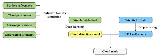
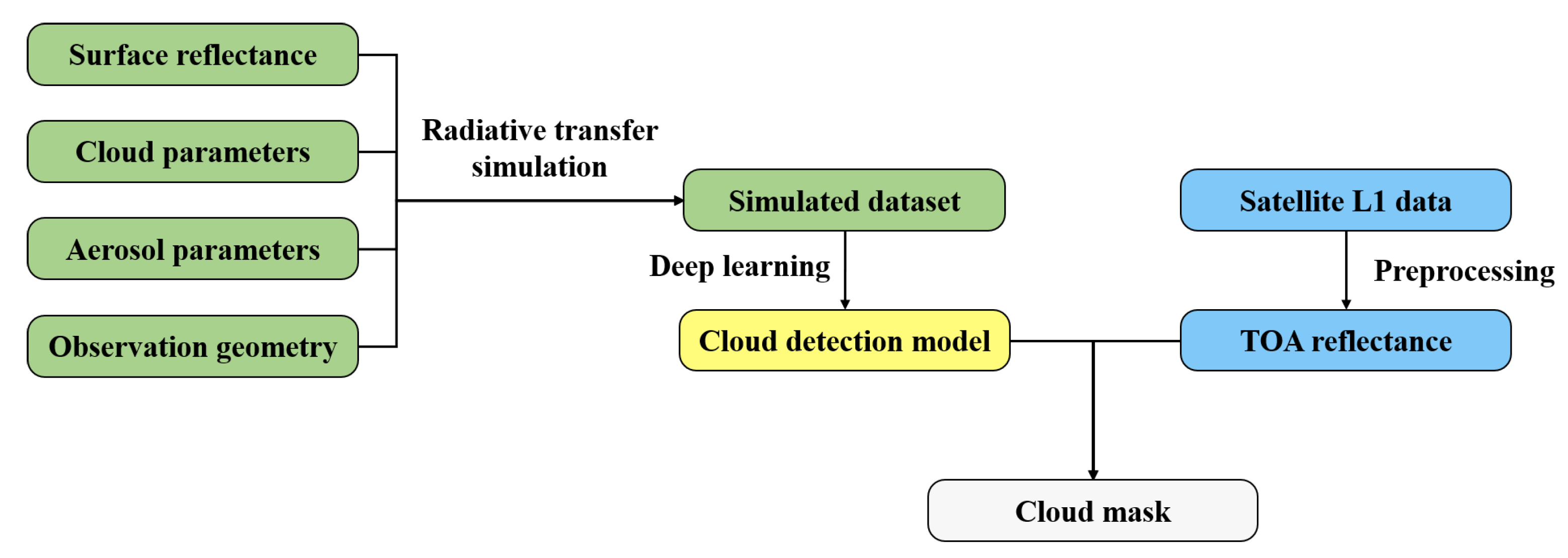
In this section, we provide a detailed introduction to the RTCD method workflow, including the radiative transfer model, the data required for simulation, dataset construction, and the design of the neural network. The flowchart of the RTCD method is shown in Figure 2. The cloud phase includes ice clouds and water clouds, while the aerosol types comprise rural, oceanic, and tropospheric aerosols.
Figure 2.
Flowchart of the RTCD method.
2.1. Radiative Transfer Model
In this paper, we used SBDART (Santa Barbara DISORT Atmospheric Radiative Transfer, https://github.com/paulricchiazzi/SBDART, accessed on 13 March 2026) to simulate the apparent reflectance under given inputs. SBDART is a software developed by Ricchiazzi et al. [27] for calculating parallel plane radiation transfer under clear and cloudy conditions. SBDART can simulate radiative transfer in cloudy atmospheres and has a wide range of applications, such as cloud optical depth [28] and aerosol radiative forcing [29,30]. Therefore, SBDART is well-suited to meet the requirements of this study. The radiative transfer equation under the condition of plane-parallel at a given wavelength is [31]
where is the radiance of the radiation along the direction at . is the cosine of the polar angle, is the azimuthal angle, and is the optical depth calculated downwards from the top of the atmosphere. S is the source function:
where is the single-scattering albedo and is the phase function, which describes the probability distribution of a photon being scattered from incident direction into direction . is the source term for a parallel beam striking a non-emitting medium from direction , .
Since SBDART does not directly output the apparent reflectance, we use the following formula to calculate the apparent reflectance:
where I is the radiance at the top of the atmosphere simulated by the radiative transfer model under given inputs, and is the solar irradiance at the top of the atmosphere, which can be obtained from the output of the radiative transfer model. is the cosine of the user-defined solar zenith angle.
2.2. Surface Reflectance
In order to make our simulated dataset closer to reality, it is crucial to obtain spatially continuous surface reflectance. During the training of cloud detection models, the model learns the deep semantic features of the clear sky surfaces or the clouds. The contextual information and texture features of the whole image provided by the spatially continuous reflectance are crucial for the accuracy of cloud detection. In order to obtain the required surface reflectance for the experiment, we used the MOD09A1 surface reflectance product, which is synthesized from MODIS data every eight days and provides seven bands of surface reflectance after atmospheric correction. MOD09A1 can be applied to aerosol quantitative retrieval [32,33], carbon emission and environmental monitoring [34], and land cover classification [35], demonstrating its strong versatility. Therefore, we selected it as the surface reflectance product for this study.
2.3. Cloud
Consistent with the principle for selecting the surface reflectance product, we use the MODIS cloud product (MOD06) as the input cloud parameters for the simulated data to simulate the contextual and textural information in real remote sensing data as fully as possible.
2.4. Simulation Results
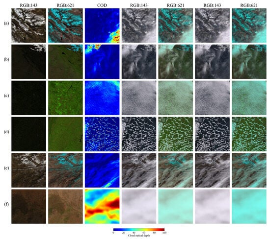
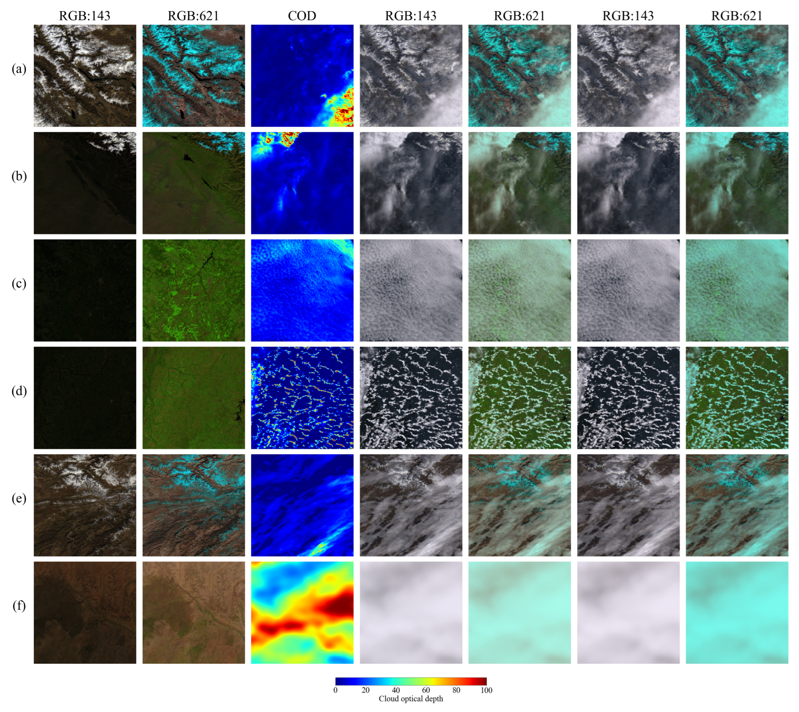
The data we select from MOD09A1 covers various surface types include bare land, vegetation, snow, and mixtures of different surface types. We combine them with different cloud optical depths to generate a simulated dataset. The range of each parameter is shown in Table 1. Figure 3 shows some of the simulated images. It should be noted that we not only display the false-color images synthesized from MOD09A1 bands 6, 2, and 1 used for training the neural network, but also present, for comparison, the true-color images synthesized from MOD09A1 bands 1, 4, and 3 (with wavelength ranges of 0.620–0.670 m, 0.545–0.565 m, and 0.459–0.479 m, corresponding to the red, green, and blue bands, respectively). The underlying surface types in the pictures include snow, bare land and vegetation.
Table 1.
Parameters and their ranges in the simulated data.
Figure 3.
Figures (a–f) present the simulation results. The images contain some typical types of underlying surfaces and cloud types. The underlying surface types include snow, bare land, vegetation, and water. The cloud types include thick clouds, thin clouds, and broken clouds. From left to right: True-color images composed of MOD09A1 bands 1, 4, and 3; false color images composed of MOD09A1 bands 6, 2, and 1; cloud optical depths; true-color images composed of MOD09A1 bands 1, 4, and 3 when clouds are in the liquid phase; false-color images composed of MOD09A1 bands 6, 2, and 1 when clouds are in the liquid phase; true-color image composed of MOD09A1 bands 1, 4, and 3 when clouds are in the ice phase; false-color image composed of MOD09A1 bands 6, 2, and 1 when clouds are in the ice phase.
2.5. Training of the Cloud Detection Models
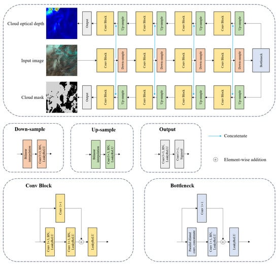
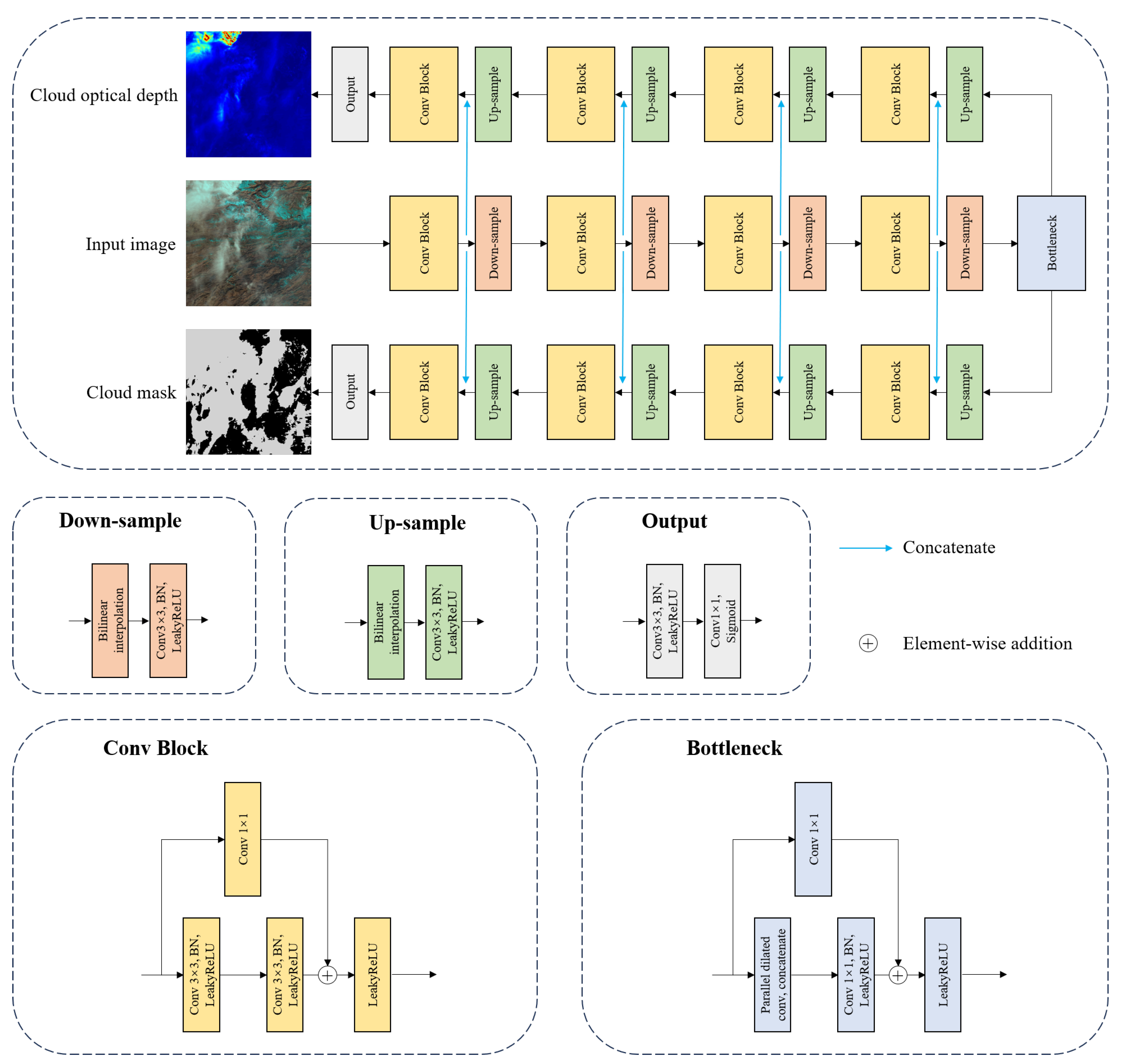
In this study, we treated cloud detection as an image segmentation task. Pixels in the remote sensing images are classified into two categories: cloud and cloud-free. Some of the simulated images are presented in Figure 3. We proposed a specialized network architecture, as illustrated in Figure 4. The network employs a dual-decoder design: two task-specific decoders share a common encoder, facilitating the cross-task sharing of low-level features.
Figure 4.
The network architecture used in this study. Black arrows represent the outputs and inputs of the modules, while rectangles of different colors denote different modules.
In terms of the loss function, we adopted a multi-task framework that includes losses for cloud mask prediction and cloud optical depth (COD) prediction. The total loss is the weighted sum of the two component losses:
where and are weighting coefficients. The cloud mask loss combines Binary Cross-Entropy (BCE) loss and Dice loss:
where denotes the ground-truth binary label, represents the predicted probability for pixel i, and N is the total number of pixels.
The COD loss incorporates four components:
They are introduced below.
The L1 reconstruction loss measures the pixel-wise absolute difference between the predicted COD and the ground truth:
where and denote the predicted and ground-truth COD values at pixel i, respectively. This loss component ensures accurate value estimation at each pixel location while being robust to outliers compared to L2 loss.
To preserve fine edge structures and boundaries in the COD prediction, we introduce the gradient edge loss:
To capture structural discrepancies across different spatial scales, we employ the Laplacian pyramid decomposition loss:
where denotes the k-th level of the Laplacian pyramid decomposition. is the scale-dependent weighting factor. K represents the total number of pyramid levels. and represent the ground-truth COD and predicted COD respectively. This multi-scale approach enables the model to simultaneously learn both fine-grained local details and global structural patterns.
To specifically address false-positive predictions in cloud-free regions, we incorporate a background-aware Binary Cross-Entropy loss:
where denotes the set of pixel indices belonging to the background region in the ground truth. This loss term penalizes non-zero predictions in areas where the ground truth indicates completely cloud-free conditions, thereby significantly suppressing the network’s prediction errors in non-cloud regions. In the experiments conducted in this paper, we set the ratio : to 20:1, the ratio : to 1:1, and the ratio ::: to 10:5:1:10.
3. Experimental Results and Analysis
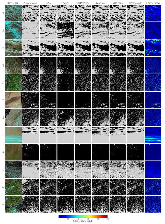
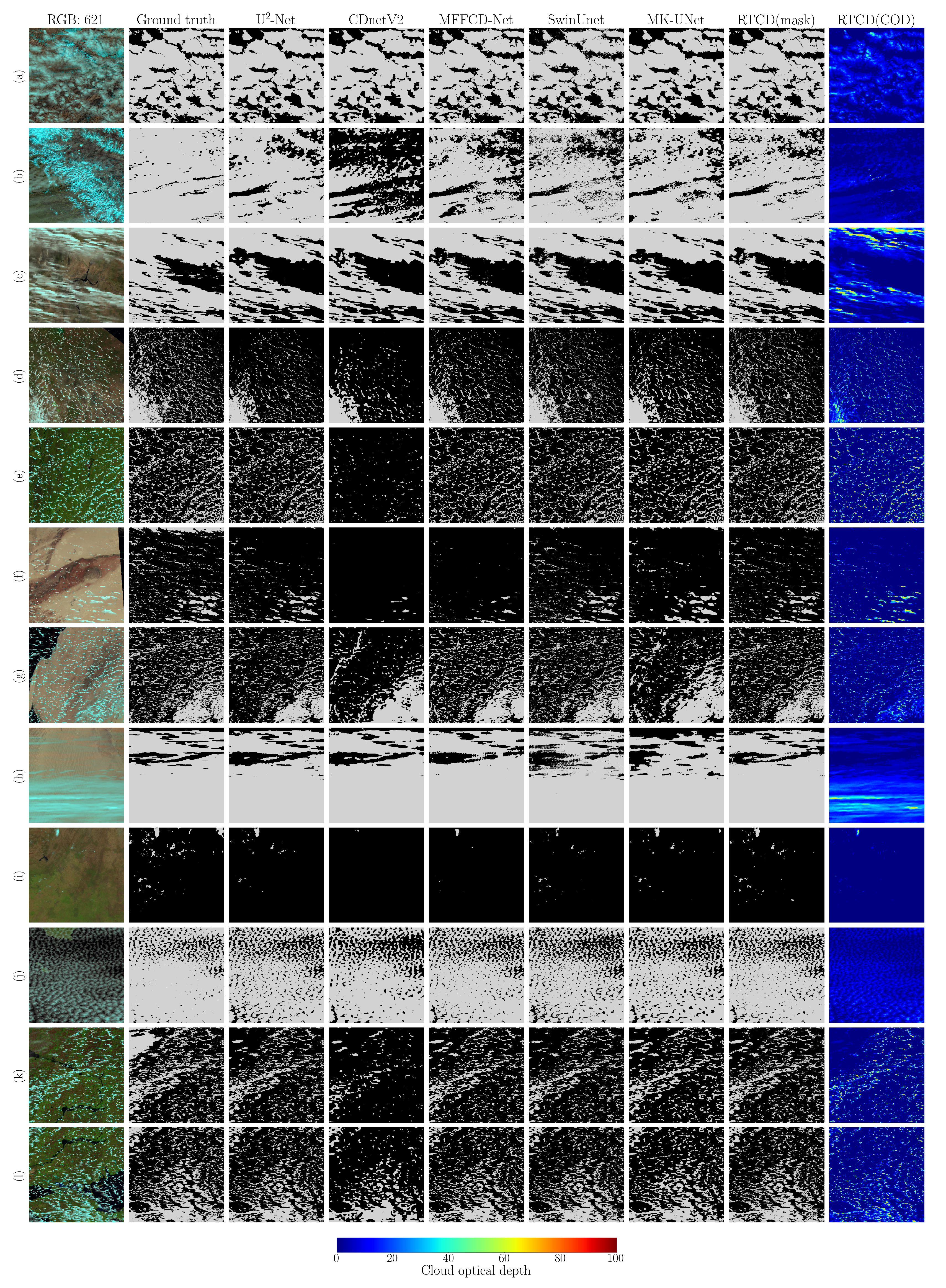
In this section, we conducted cloud detection experiments on both the simulated dataset and real satellite imagery (MODIS, MERSI-RM) using different methods and performed a comparative analysis of the results. We selected -Net [36], CDnetV2 [37], MFFCD-Net [25], SwinUnet [38], and MK-UNet [39] as the networks for training the cloud detection models on the simulated dataset. It should be noted that we trained Net, CDnetV2, MFFCD-Net, SwinUnet, and MK-UNet not only on our simulated dataset but also on the Landsat 8 CCA (Cloud Cover Assessment) dataset [16,40] for comparative analysis. The results of networks trained on this dataset are marked with an asterisk (*) after the network name in the figures and tables of the paper. The network we proposed was not trained on this dataset because the dataset does not contain cloud optical depth information. Some of the results are shown in Figure 5, and quantitative accuracy assessments are presented in Table 3.
Figure 5.
Figures (a–l) present the results on the simulated data. The images contain some typical types of underlying surfaces and cloud types. The underlying surface types include snow, bare land, vegetation, and water. The cloud types include thick clouds, thin clouds, and broken clouds. For all cloud detection results, light gray represents clouds, and black represents clear sky. “RGB: 621” represents false-color image composed of MOD09A1 bands 6, 2, and 1; “Ground truth” represents manually annotated cloud mask; the other columns represent the outputs of different neural networks. It should be noted that “RTCD(COD)” represents the cloud optical depth generated by the RTCD method.
We selected some MODIS images and MERSI-RM images to validate the cloud detection performance of different methods on real satellite imagery. The spectral bands of the data we used are shown in Table 2. These images, along with their corresponding cloud detection results, are provided in Figure 6 and Figure 7, and quantitative accuracy assessments are presented in Tables 4 and 5.
Table 2.
Spectral bands of the data used.
Figure 6.
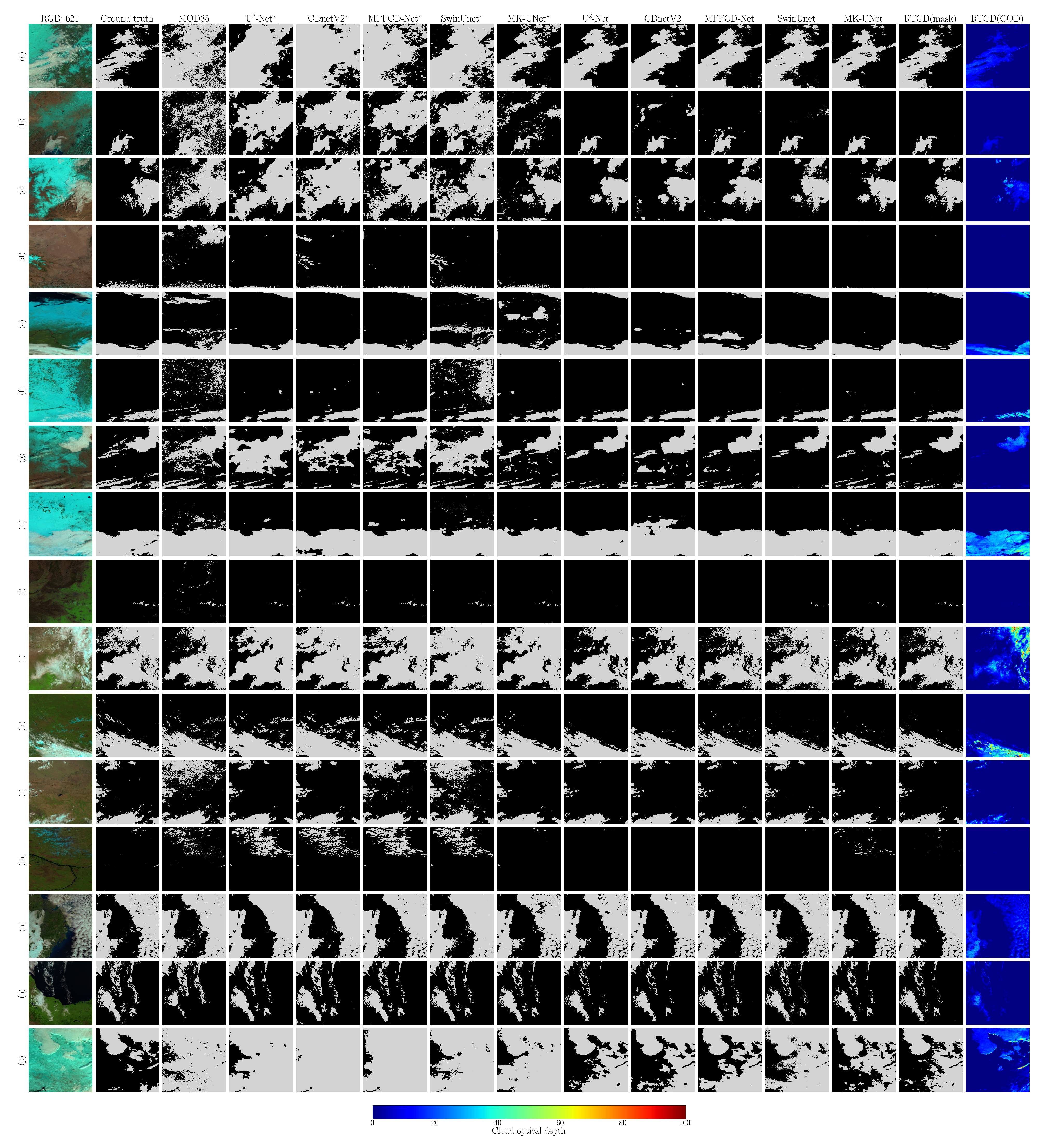
Figures (a–p) present the results on MODIS data. For all cloud detection results, light gray represents clouds and black represents clear sky. “RGB: 621” represents false-color image composed of MODIS bands 6, 2, and 1; “Ground truth” represents manually annotated cloud mask; “MOD35” represents the MODIS cloud mask product (MOD35), where light gray represents “cloudy” and black represents “uncertain clear”, “probably clear”, and “confident clear”; the other columns represent the outputs of different neural networks. Those marked with an asterisk (*) indicate that the neural network was trained on the Landsat 8 CCA dataset, while those without an asterisk were trained on the simulated dataset. It should be noted that “RTCD(COD)” represents the cloud optical depth generated by the RTCD method.
Figure 7.
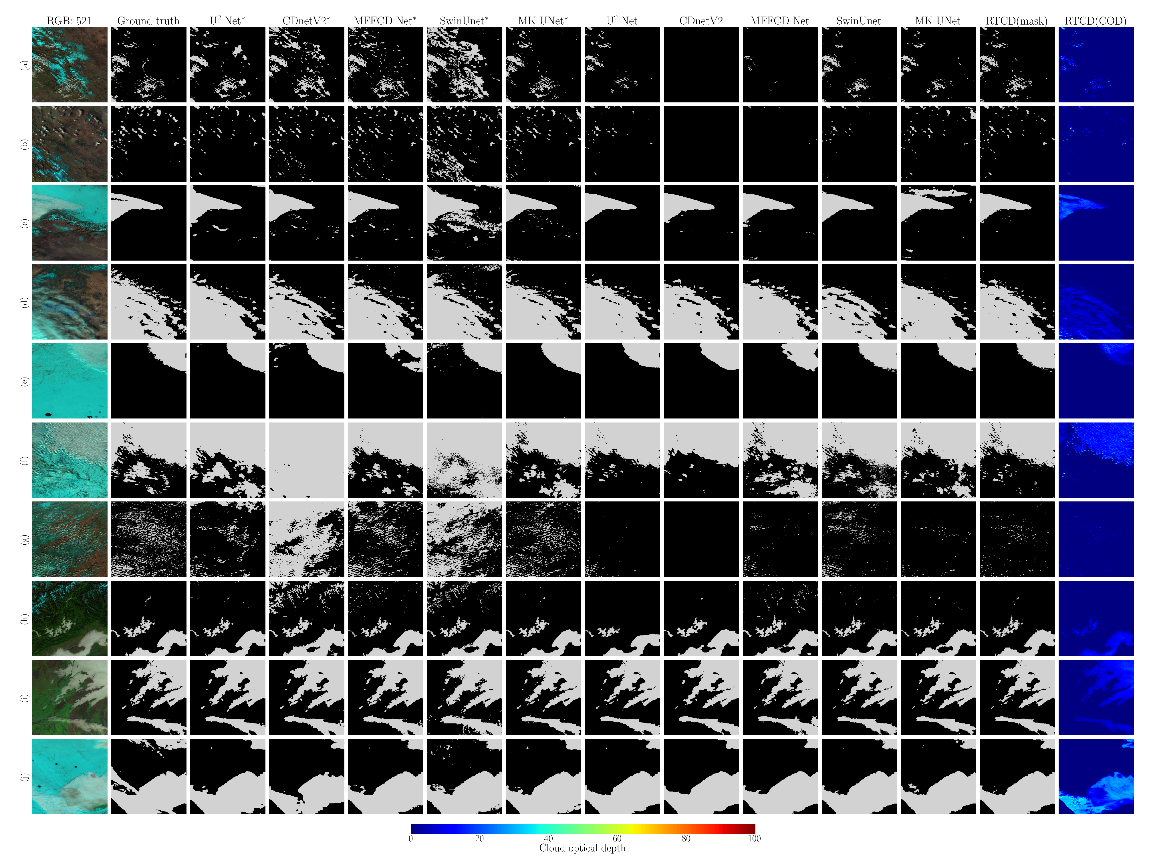
Figures (a–j) present the results on MERSI-RM data. For all cloud detection results, light gray represents clouds and black represents clear sky. “RGB: 521” represents false-color image composed of MERSI-RM bands 5, 2, and 1; “Ground truth” represents manually annotated cloud mask; The other columns represent the outputs of different neural networks. Those marked with an asterisk (*) indicate that the neural network was trained on the Landsat 8 CCA dataset, while those without an asterisk were trained on the simulated dataset. It should be noted that “RTCD(COD)” represents the cloud optical depth generated by the RTCD method.
3.1. Evaluation Metrics
We manually annotated cloud masks on MODIS data and MERSI-RM data as ground truth for comparison with the experimental results of different methods. We select the hit rate, missing rate, error rate, and F1 score as the cloud detection accuracy evaluation metrics, which are defined as follows:
where
and
True positive (TP) represents the number of pixels classified as cloudy by both the reference mask and the cloud detection result. True negative (TN) represents the number of pixels classified as clear by both the reference mask and the cloud detection result. False positive (FP) represents the number of pixels classified as clear by the reference mask but classified as cloudy by the cloud detection result. False negative (FN) represents the number of pixels classified as cloudy by the reference data but classified as clear by the cloud detection result. Table 3, Table 4 and Table 5 show the quantitative accuracy evaluation of different methods on the simulated data, MODIS data, and MERSI-RM data respectively.
When calculating the missing rate, error rate, and F1 score, the value of the denominator may be zero, which leads to meaningless results. We adopt the following criterion to handle such cases: if the denominator for the missing rate or error rate is zero, we return a value of 0. A zero denominator in the missing rate or error rate indicates that their numerator (FN or FP) is also zero, meaning that no cloud pixels were falsely detected as clear sky, or no clear sky pixels were falsely detected as clouds. Thus, the missing rate or error rate is set to 0. The F1 score is calculated based on precision and recall. If the denominator of precision or recall is zero, this implies that their numerator (TP) is also zero, indicating that no cloud pixels were correctly detected. In this case, the F1 score is set to 0.
3.2. Experimental Results on the Simulated Data
We first evaluated the performance of different networks on the simulated dataset, which consists of 1000 training images and 900 test images. The cloud detection results are summarized in Table 3. As shown in Table 3, our method achieved a hit rate, missing rate, error rate, and F1 score of 97.06%, 5.83%, 0.29%, and 96.84%, respectively, on the simulated dataset. In terms of hit rate, missing rate, and F1 score, our method outperformed the comparative methods, while its error rate ranked second, higher than that of -Net. Examples of cloud detection results on the simulated dataset are illustrated in Figure 5. From Figure 5, it can be observed that clouds over bright surfaces or fragmented clouds are prone to being missed, as particularly evident in Figure 5b,f. Although our method also missed a small number of clouds, the number of missed detections was lower than that of other methods. Misclassifications of surface features as clouds frequently occurred at the boundaries between different land cover types, such as the land-sea interface in the upper-left corner of Figure 5g, whereas our method exhibited almost no false alarms in this region. Overall, our method achieved excellent results across all evaluation metrics and demonstrated the best comprehensive performance among the compared methods.
Table 3.
Quantitative evaluation of cloud detection results of different methods on the simulated data.
3.3. MODIS Experimental Results
Figure 6 shows the cloud detection results on MODIS data. The false-color images are composed of MODIS bands 6, 2, and 1. In the false-color images, clouds appear white or light cyan, while snow appears cyan. MOD35 is the cloud mask product of MODIS. The algorithm for producing this product is described by Ackerman et al. [4] and Frey et al. [41]. In order to evaluate the accuracy of the cloud detection methods, the corresponding MOD35 product was selected for comparison.
Figure 6a–c shows a comparison of the cloud detection results in winter near Northeast China. As can be seen in the images, the surface is a mixture of snow, bare land, and vegetation. The spectral characteristics of this type of surface are very similar to those of cloud and could be misjudged as clouds. This type of surface represents the key and difficult part of the cloud detection tasks. Figure 6d shows the Loess Plateau region of China, with a broken thin cirrus cloud at the bottom of the picture. Figure 6e shows the Ob River Basin. The composition of the underlying surface in this scene includes snow, vegetation, sea water and sea ice. The underlying surface of Figure 6f is snow and vegetation. Figure 6g shows a scene in the north central United States, where the underlying surface consists of snow mixed with bare land, covered by a thin layer of clouds. Figure 6h shows the cloud detection results over northern Kazakhstan, where the surface is almost entirely covered by snow. Figure 6i shows the detection results of thin cirrus clouds near the Taihang Mountains in China. Figure 6j shows the Loess Plateau in China. The clouds in the upper left corner of the picture are thin and broken, and the underlying surface is bare land and vegetation. Figure 6k shows Eastern Siberia. Figure 6l shows Northeast India, where the underlying surface is composed of bare land and vegetation, covered by a small number of thin and broken clouds. Figure 6m shows Lena River Basin. Figure 6n shows Zhejiang Province, China, and the East China Sea. Figure 6o shows the cloud detection results in the southern Gulf of Mexico. Figure 6p shows the cloud detection results over southern Canada, where the underlying surface is almost entirely snow-covered.
Table 4.
Quantitative evaluation of cloud detection results from different methods on MODIS data. Model names marked with an asterisk (*) indicate that the corresponding models were trained on the Landsat 8 CCA dataset.
We can summarize from Figure 6 and Table 4 that our method generally demonstrates higher accuracy than the MOD35 product and other deep learning methods trained on the cloud detection datasets. In some scenarios, our results show a higher missing rate but a lower error rate compared to the MOD35 product. This indicates that, while the MOD35 product has higher sensitivity to clouds, it also misclassifies a large number of bright surfaces, particularly those with mixed snow and bare land, as clouds. However, it should be noted that the MOD35 product occasionally misses cloud pixels. The reason why some deep learning methods, including ours, are less likely to misclassify surfaces mixed with snow and bare land as clouds is that the textural and deep semantic features of these bright surfaces are distinct from those of clouds. These differences can be captured by neural networks to distinguish them from clouds. The accuracy of networks trained on the Landsat 8 CCA dataset is lower than that of networks trained on our simulated dataset. This is primarily because the Landsat 8 CCA dataset contains relatively few mixed surface types of snow and bare land. This limitation results in models trained on this dataset being unable to effectively learn the spectral and textural features of such surfaces, leading to the misclassification of a large number of these surface pixels as clouds.
3.4. MERSI-RM Experimental Results
Figure 7 shows the cloud detection results on MERSI-RM data. The underlying surfaces of the scenes in Figure 7 are mainly composed of snow and bare land. The clouds in Figure 7a,b are broken and scattered, and the underlying surface is an irregular mixture of snow and bare land. The scene shown in Figure 7c is in Northwest China. The area shown in Figure 7d is located in the northern part of the Aral Sea. Figure 7e shows the cloud detection results over southwestern Russia in winter. Figure 7f shows thin and thick clouds covering snow. The area displayed in Figure 7g is located in the southeast of Lake Baikal, with thin and broken clouds. The regions in Figure 7h,i are located in the Qinghai-Tibet Plateau and northern India respectively. The snow-covered area in Figure 7j is located in central and southern Russia and is covered by thin clouds.
The cloud detection results of networks trained on the Landsat 8 CCA dataset exhibit greater instability compared to those of networks trained on the simulated dataset. The reason for this is consistent with the explanation previously provided for the cloud detection results on MODIS imagery, i.e., the Landsat 8 CCA dataset contains relatively few mixed snow and bare land surface types. A more detailed discussion can be found in Section 4.
Table 5.
Quantitative evaluation of cloud detection results from different methods on MERSI-RM data. Model names marked with an asterisk (*) indicate that the corresponding models were trained on the Landsat 8 CCA dataset.
3.5. Ablation Experiment
To validate the impact of the dual-decoder in the proposed network, we conducted an ablation experiment on the simulated dataset. Table 6 presents a comparison of the performance from the ablation experiment. As can be seen from the table, after incorporating the COD branch, the model’s performance in hit rate, missing rate, and F1 score improved. However, the error rate is inferior to the performance when using the cloud mask branch alone. This indicates that the COD branch enhances the model’s sensitivity to clouds but also introduces a higher rate of false positives.
Table 6.
Cloud detection accuracy of the ablation experiments.
4. Discussion
As shown in Table 4 and Table 5, our method demonstrates higher overall detection accuracy compared to the MOD35 product, particularly in snow and bare land areas. This improvement stems from the fact that our algorithm utilizes not only the spectral reflectance characteristics of clouds but also their textural features to distinguish between cloudy and cloud-free regions. In high-altitude or high-latitude regions with extremely low temperatures, the surface is typically composed of bare land or snow. These surfaces exhibit low brightness temperatures and high reflectance, closely resembling the spectral characteristics of clouds. However, their textural features differ significantly from those of clouds. The MOD35 product performs pixel-by-pixel cloud detection and cannot utilize textural features to distinguish between clouds and non-cloud regions; thus, it exhibits high error rates in these areas. Our method, on the other hand, fully leverages textural features, enabling higher accuracy in cloud detection over high-altitude or high-latitude regions. The cloud detection models trained on the Landsat 8 CCA dataset generally show lower cloud detection accuracy on both MODIS and MERSI-RM data compared to the cloud detection models trained on our simulated dataset, especially on the MODIS data. This is because the Landsat 8 CCA dataset encompasses a less diverse range of surface types compared to our simulated dataset. In particular, the L8 CCA dataset lacks a sufficient representation of mixed snow and bare land surfaces, which are prone to being misclassified as clouds and constitute one of the challenging aspects in cloud detection. However, the L8 CCA dataset also offers unique advantages over our simulated dataset, which is elaborated upon subsequently. In the areas with thin cloud cover, such as the scenarios illustrated in Figure 6d and Figure 7g, our method exhibits a higher rate of missed detections for very fragmented clouds compared to MOD35 or cloud detection models trained on the Landsat 8 CCA dataset. Other cloud detection models trained on our simulated dataset also show a similar trend. This is because thin clouds or small, fragmented clouds over surfaces often exhibit spectral reflectance features similar to those of bright surfaces, and the textural features of thin clouds are less pronounced compared to thick clouds. The MOD35 product employs a complex detection process, including visible, infrared, and thermal infrared bands, to perform pixelwise cloud detection on MODIS data. Since thermal infrared bands are highly sensitive to clouds, the MOD35 product can detect more thin clouds. In contrast, our method utilizes only visible and shortwave infrared bands for cloud detection and does not incorporate thermal infrared bands, resulting in relatively weaker detection capability for thin clouds and thus a higher missing rate compared to the MOD35 product. Furthermore, for cloud detection tasks, cloud shadows serve as a crucial indicator for identifying clouds. In the absence of thermal infrared channels, certain extremely thin clouds, such as cirrus clouds, are particularly challenging to distinguish. In such scenarios, cloud shadows play a crucial role in cloud detection, as they are often more discernible than the clouds themselves in remote sensing imagery. Moreover, cloud shadows typically accompany clouds and exhibit a high degree of shape consistency with them. Additionally, cloud shadows and clouds display a distinct spatial relationship, which is governed by observation geometry and the height of the clouds above the ground. In real remote sensing datasets, such as the Landsat 8 CCA dataset, the aforementioned relationship between cloud shadows and clouds is authentically represented. This relationship can be effectively captured by cloud detection models trained on real remote sensing datasets, thereby significantly reducing the missing rate for thin and fragmented clouds. In contrast, although our simulated dataset can accurately replicate the clouds in remote sensing images, it does not incorporate the simulation of cloud shadows. Consequently, cloud detection models trained on our simulated dataset are more prone to missing thin and fragmented clouds compared to those trained on real remote sensing datasets.
5. Conclusions
For most remote sensing applications, cloud detection is a crucial preprocessing step. This study proposed a novel cloud detection method that integrates radiative transfer with deep learning. First, we constructed a cloud detection dataset. Unlike other datasets, our cloud detection dataset is entirely simulation-based rather than manually labeled from real remote sensing cloud images. Specifically, we input existing remote sensing products, such as surface reflectance and cloud optical depth products, into the radiative transfer model to generate simulated images. These remote sensing products and the radiative transfer model are widely used in quantitative remote sensing, ensuring that the simulated remote sensing images have practical physical significance. Subsequently, we proposed a neural network for training a cloud detection model on the simulated dataset. The experimental results on MODIS and MERSI-RM imagery show that our method achieves satisfactory results, particularly in areas with mixed snow and bare land, where its performance is significantly better than that of MOD35, demonstrating the effectiveness of our method.
In conclusion, our method provides a new perspective for cloud detection, particularly for supervised deep learning based approaches. The main contributions of this paper are summarized as follows:
- 1.
- A method for constructing cloud detection datasets based on radiative transfer models, existing surface reflectance products, and cloud optical depth products has been proposed. This approach eliminates the need for the extensive manual labeling of training data, allowing models to be trained on simulated datasets to perform cloud detection tasks. Since surface reflectance products cover the globe and cloud optical depth products include various cloud formations, any combination of surface and cloud types can be utilized to produce corresponding simulated images, significantly increasing the diversity of the dataset.
- 2.
- We trained different neural network models for cloud detection, including -Net, CDnetV2, MFFCD-Net, SwinUnet, MK-Unet, and the network we proposed on the simulated dataset. We evaluated the cloud detection performance of these networks on both simulated images and real satellite images. The experimental results demonstrate that the network we proposed outperforms other networks. Additionally, we compared the results with the networks trained on the Landsat 8 CCA dataset. The experimental results show that the networks trained on our simulated dataset exhibit greater stability. The simulated dataset generation method we proposed partially alleviates the scarcity of cloud detection datasets, especially for specific satellite sensors, such as MODIS.
However, there is still significant room for improvement in our method:
- 1.
- We assume the surface to be Lambertian. In future work, the non-Lambertian reflection characteristics of the surface should also be taken into account. We plan to integrate the MCD43 product, which provides global anisotropic kernel parameters, to characterize the angular dependence of surface reflectance. This approach would make the simulated dataset more realistic.
- 2.
- Cloud shadows. When the solar zenith angle is large, cloud shadows in remote sensing images are often obvious. As is discussed in Section 4, cloud shadows in remote sensing imagery can assist in cloud detection and enhance the model’s ability to detect thin and fragmented clouds. In addition, according to [42], cloud shadows can obscure remote sensing images, making it difficult to utilize these regions for remote sensing retrievals. Current methods for detecting cloud shadows primarily include spectral analysis and deep learning techniques, such as [42,43,44,45]. In future work, we plan to explore feasible methods for simulating cloud shadows, which would not only enhance cloud detection accuracy but also enable the models to detect cloud shadows, thereby providing robust support for subsequent remote sensing products.
- 3.
- In this paper, only the reflection spectral bands were simulated and the thermal infrared bands were not used, which limits our method’s ability to detect extremely thin clouds. Previous cloud detection research has shown that thermal infrared bands also have good cloud detection effectiveness, especially for the detection of high and thin clouds (such as cirrus) [46]. Moreover, the thermal infrared bands also have the ability to detect clouds at night, which can enhance the applicability of our cloud detection method.
Author Contributions
Conceptualization, M.G. and Y.H.; methodology, Z.H. and B.L.; software, Z.H. and B.L.; writing—original draft preparation, Z.H.; investigation, F.Z. and L.L.; data curation, F.Z., L.L. and Z.H.; writing—review and editing, M.G. and Y.H.; funding acquisition, M.G. All authors have read and agreed to the published version of the manuscript.
Funding
This work was funded by the National Key Research and Development Program of China under Grant 2023YFB3905401.
Data Availability Statement
This study analyzed publicly available datasets. The data can be accessed as follows: 1. MODIS data employed in this study is sourced from https://search.earthdata.nasa.gov/ (accessed on 16 September 2025). 2. MERSI-RM data employed in this study is sourced from http://www.nsmc.org.cn/nsmc/cn/home/index.html (accessed on 16 September 2025). 3. Landsat 8 Cloud Cover Assessment dataset employed in this study is sourced from https://landsat.usgs.gov/landsat-8-cloud-cover-assessment-validation-data (accessed on 1 October 2025).
Conflicts of Interest
The authors declare no conflicts of interest.
References
- Harshvardhan; Randall, D.A.; Corsetti, T.G. Earth Radiation Budget and Cloudiness Simulations with a General Circulation Model. J. Atmos. Sci. 1989, 46, 1922–1942. [Google Scholar] [CrossRef] [Scilit]
- King, M.D.; Platnick, S.; Menzel, W.P.; Ackerman, S.A.; Hubanks, P.A. Spatial and Temporal Distribution of Clouds Observed by MODIS Onboard the Terra and Aqua Satellites. IEEE Trans. Geosci. Remote Sens. 2013, 51, 3826–3852. [Google Scholar] [CrossRef] [Scilit]
- Koren, I.; Oreopoulos, L.; Feingold, G.; Remer, L.A.; Altaratz, O. How small is a small cloud? Atmos. Chem. Phys. 2008, 8, 3855–3864. [Google Scholar] [CrossRef] [Scilit]
- Ackerman, S.A.; Strabala, K.I.; Menzel, P.W.; Frey, R.A.; Moeller, C.C.; Gumley, L.; Baum, B.A.; Seemann, S.W.; Zhang, H. Discriminating clear sky from clouds with MODIS. J. Geophys. Res. 1998, 103, 32141–32157. [Google Scholar] [CrossRef] [Scilit]
- Ali, A.; de Bie, C.; Skidmore, A. Detecting long-duration cloud contamination in hyper-temporal NDVI imagery. Int. J. Appl. Earth Obs. Geoinf. 2013, 24, 22–31. [Google Scholar] [CrossRef] [Scilit]
- Pu, W.; Wang, Z.; Liu, D.; Zhang, Q. Optical Remote Sensing Image Cloud Detection with Self-Attention and Spatial Pyramid Pooling Fusion. Remote Sens. 2022, 14, 4312. [Google Scholar] [CrossRef] [Scilit]
- Sakaida, F.; Hosoda, K.; Moriyama, M.; Murakami, H.; Mukaida, A.; Kawamura, H. Sea surface temperature observation by Global Imager (GLI)/ADEOS-II: Algorithm and accuracy of the product. J. Oceanogr. 2006, 62, 311–319. [Google Scholar] [CrossRef] [Scilit]
- Gesell, G. An algorithm for snow and ice detection using AVHRR data An extension to the APOLLO software package. Int. J. Remote Sens. 1989, 10, 897–905. [Google Scholar] [CrossRef] [Scilit]
- Stowe, L.; McClain, E.; Carey, R.; Pellegrino, P.; Gutman, G.; Davis, P.; Long, C.; Hart, S. Global distribution of cloud cover derived from NOAA/AVHRR operational satellite data. Adv. Space Res. 1991, 11, 51–54. [Google Scholar] [CrossRef] [Scilit]
- Rossow, W.B.; Garder, L.C. Cloud Detection Using Satellite Measurements of Infrared and Visible Radiances for ISCCP. J. Clim. 1993, 12, 2341–2369. [Google Scholar] [CrossRef] [Scilit]
- Irish, R.R. Landsat 7 automatic cloud cover assessment. In Proceedings of the Algorithms for Multispectral, Hyperspectral, and Ultraspectral Imagery VI; Shen, S.S., Descour, M.R., Eds.; International Society for Optics and Photonics, SPIE: Bellingham, WA, USA, 2000; Volume 4049, pp. 348–355. [Google Scholar] [CrossRef] [Scilit]
- Irish, R.R.; Barker, J.L.; Goward, S.N.; Arvidson, T. Characterization of the Landsat-7 ETM+ Automated Cloud-Cover Assessment (ACCA) Algorithm. Photogramm. Eng. Remote Sens. 2006, 72, 1179–1188. [Google Scholar] [CrossRef] [Scilit]
- Luo, Y.; Trishchenko, A.P.; Khlopenkov, K.V. Developing clear-sky, cloud and cloud shadow mask for producing clear-sky composites at 250-meter spatial resolution for the seven MODIS land bands over Canada and North America. Remote Sens. Environ. 2008, 112, 4167–4185. [Google Scholar] [CrossRef] [Scilit]
- Oreopoulos, L.; Wilson, M.J.; Várnai, T. Implementation on Landsat Data of a Simple Cloud-Mask Algorithm Developed for MODIS Land Bands. IEEE Geosci. Remote Sens. Lett. 2011, 8, 597–601. [Google Scholar] [CrossRef] [Scilit]
- Zhu, Z.; Woodcock, C.E. Object-based cloud and cloud shadow detection in Landsat imagery. Remote Sens. Environ. 2012, 118, 83–94. [Google Scholar] [CrossRef] [Scilit]
- Foga, S.; Scaramuzza, P.L.; Guo, S.; Zhu, Z.; Dilley, R.D.; Beckmann, T.; Schmidt, G.L.; Dwyer, J.L.; Joseph Hughes, M.; Laue, B. Cloud detection algorithm comparison and validation for operational Landsat data products. Remote Sens. Environ. 2017, 194, 379–390. [Google Scholar] [CrossRef] [Scilit]
- Qiu, S.; Zhu, Z.; He, B. Fmask 4.0: Improved cloud and cloud shadow detection in Landsats 4–8 and Sentinel-2 imagery. Remote Sens. Environ. 2019, 231, 111205. [Google Scholar] [CrossRef] [Scilit]
- Wei, J.; Sun, L.; Jia, C.; Yang, Y.; Zhou, X.; Gan, P.; Jia, S.; Liu, F.; Li, R. Dynamic threshold cloud detection algorithms for MODIS and Landsat 8 data. In Proceedings of the 2016 IEEE International Geoscience and Remote Sensing Symposium (IGARSS), Beijing, China, 10–15 July 2016; pp. 566–569. [Google Scholar] [CrossRef] [Scilit]
- Mazzoni, D.; Garay, M.J.; Davies, R.; Nelson, D. An operational MISR pixel classifier using support vector machines. Remote Sens. Environ. 2007, 107, 149–158. [Google Scholar] [CrossRef] [Scilit]
- Yuan, Y.; Hu, X. Bag-of-Words and Object-Based Classification for Cloud Extraction From Satellite Imagery. IEEE J. Sel. Top. Appl. Earth Obs. Remote Sens. 2015, 8, 4197–4205. [Google Scholar] [CrossRef] [Scilit]
- Wei, J.; Huang, W.; Li, Z.; Sun, L.; Zhu, X.; Yuan, Q.; Liu, L.; Cribb, M. Cloud detection for Landsat imagery by combining the random forest and superpixels extracted via energy-driven sampling segmentation approaches. Remote Sens. Environ. 2020, 248, 112005. [Google Scholar] [CrossRef] [Scilit]
- Li, Z.; Shen, H.; Cheng, Q.; Liu, Y.; You, S.; He, Z. Deep learning based cloud detection for medium and high resolution remote sensing images of different sensors. ISPRS J. Photogramm. Remote Sens. 2019, 150, 197–212. [Google Scholar] [CrossRef] [Scilit]
- Yang, J.; Guo, J.; Yue, H.; Liu, Z.; Hu, H.; Li, K. CDnet: CNN-Based Cloud Detection for Remote Sensing Imagery. IEEE Trans. Geosci. Remote Sens. 2019, 57, 6195–6211. [Google Scholar] [CrossRef] [Scilit]
- Segal-Rozenhaimer, M.; Li, A.; Das, K.; Chirayath, V. Cloud detection algorithm for multi-modal satellite imagery using convolutional neural-networks (CNN). Remote Sens. Environ. 2020, 237, 111446. [Google Scholar] [CrossRef] [Scilit]
- Li, J.; Hu, C.; Sheng, Q.; Wang, B.; Ling, X.; Gao, F.; Xu, Y.; Li, Z.; Molinier, M. A Unified Cloud Detection Method for Suomi-NPP VIIRS Day and Night PAN Imagery. IEEE Trans. Geosci. Remote Sens. 2024, 62, 1–13. [Google Scholar] [CrossRef] [Scilit]
- Sun, L.; Yang, X.; Jia, S.; Jia, C.; Wang, Q.; Liu, X.; Wei, J.; Zhou, X. Satellite data cloud detection using deep learning supported by hyperspectral data. Int. J. Remote Sens. 2020, 41, 1349–1371. [Google Scholar] [CrossRef] [Scilit]
- Ricchiazzi, P.; Yang, S. SBDART: A Research and Teaching Software Tool for Plane-Parallel Radiative Transfer in the Earth’s Atmosphere. Bull. Am. Meteorol. Soc. 1998, 79, 2101–2114. [Google Scholar] [CrossRef] [Scilit]
- Chen, Y.; Chong, K.; Fu, Y. Impacts of distribution patterns of cloud optical depth on the calculation of radiative forcing. Atmos. Res. 2019, 218, 70–77. [Google Scholar] [CrossRef] [Scilit]
- Tiwary, P.; Kukreti, S.; Shridhar, V.; Abhinav, A.; Rana, S.; Arunachalam, K.; Singh, V. Assessment of Black Carbon, optical properties and aerosol radiative forcing at Pranmati basin Himalayan critical zone observatory. Sci. Total Environ. 2024, 933, 173050. [Google Scholar] [CrossRef] [Scilit]
- Shaik, D.S.; Kant, Y.; Mitra, D.; Babu, S.S. Assessment of Aerosol Characteristics and Radiative Forcing Over Northwest Himalayan Region. IEEE J. Sel. Top. Appl. Earth Obs. Remote Sens. 2017, 10, 5314–5321. [Google Scholar] [CrossRef] [Scilit]
- Stamnes, K.; Tsay, S.C.; Wiscombe, W.; Jayaweera, K. Numerically stable algorithm for discrete-ordinate-method radiative transfer in multiple scattering and emitting layered media. Appl. Opt. 1988, 27, 2502–2509. [Google Scholar] [CrossRef] [Scilit]
- Sun, L.; Wei, J.; Jia, C.; Yang, Y.; Zhou, X.; Gan, P.; Liu, F.; Jia, S.; Li, R. A high-resolution global dataset of aerosol optical depth over land from MODIS data. In Proceedings of the 2016 IEEE International Geoscience and Remote Sensing Symposium (IGARSS), Beijing, China, 10–15 July 2016; pp. 5729–5732. [Google Scholar] [CrossRef] [Scilit]
- Wang, X.Q.; Wang, F.; Jia, L.L.; Ding, Y. Retrieval and validation of aerosol optical depth using GF-1 WFV cameras data. Adv. Space Res. 2020, 65, 997–1007. [Google Scholar] [CrossRef] [Scilit]
- Aragão, L.E.; Anderson, L.O.; Fonseca, M.G.; Rosan, T.M.; Vedovato, L.B.; Wagner, F.H.; Silva, C.V.J.; Junior, C.H.L.S.; Arai, E.; Aguiar, A.P.D.; et al. 21st Century drought-related fires counteract the decline of Amazon deforestation carbon emissions. Nat. Commun. 2018, 9, 536. [Google Scholar] [CrossRef] [Scilit] [PubMed]
- Carrão, H.; Gonçalves, P.; Caetano, M. Contribution of multispectral and multitemporal information from MODIS images to land cover classification. Remote Sens. Environ. 2008, 112, 986–997. [Google Scholar] [CrossRef] [Scilit]
- Qin, X.; Zhang, Z.; Huang, C.; Dehghan, M.; Zaiane, O.R.; Jagersand, M. U2-Net: Going deeper with nested U-structure for salient object detection. Pattern Recognit. 2020, 106, 107404. [Google Scholar] [CrossRef] [Scilit]
- Guo, J.; Yang, J.; Yue, H.; Tan, H.; Hou, C.; Li, K. CDnetV2: CNN-Based Cloud Detection for Remote Sensing Imagery with Cloud-Snow Coexistence. IEEE Trans. Geosci. Remote Sens. 2021, 59, 700–713. [Google Scholar] [CrossRef] [Scilit]
- Cao, H.; Wang, Y.; Chen, J.; Jiang, D.; Zhang, X.; Tian, Q.; Wang, M. Swin-Unet: Unet-Like Pure Transformer for Medical Image Segmentation. In Proceedings of the Computer Vision–ECCV 2022 Workshops; Karlinsky, L., Michaeli, T., Nishino, K., Eds.; Springer: Cham, Switzerland, 2023; pp. 205–218. [Google Scholar]
- Rahman, M.M.; Marculescu, R. MK-UNet: Multi-Kernel Lightweight CNN for Medical Image Segmentation. In Proceedings of the 2025 IEEE/CVF International Conference on Computer Vision Workshops (ICCVW), Honolulu, HI, USA, 19–20 October 2025; pp. 1053–1062. [Google Scholar] [CrossRef] [Scilit]
- U.S. Geological Survey. L8 Biome Cloud Validation Masks; U.S. Geological Survey: Reston, VA, USA, 2016. [Google Scholar] [CrossRef]
- Frey, R.A.; Ackerman, S.A.; Liu, Y.; Strabala, K.I.; Zhang, H.; Key, J.R.; Wang, X. Cloud Detection with MODIS. Part I: Improvements in the MODIS Cloud Mask for Collection 5. J. Atmos. Ocean. Technol. 2008, 25, 1057–1072. [Google Scholar] [CrossRef] [Scilit]
- Zhou, X.; Li, S.; Yang, J.; Wan, Y.; Sun, L.; Huang, Z. An Extended Cloud Shadow Detection Algorithm Supported by an A Priori Database. IEEE Trans. Geosci. Remote Sens. 2023, 61, 1–16. [Google Scholar] [CrossRef] [Scilit]
- Zhang, Y.; Guindon, B.; Li, X. A Robust Approach for Object-Based Detection and Radiometric Characterization of Cloud Shadow Using Haze Optimized Transformation. IEEE Trans. Geosci. Remote Sens. 2014, 52, 5540–5547. [Google Scholar] [CrossRef] [Scilit]
- Yan, Z.; Yan, M.; Sun, H.; Fu, K.; Hong, J.; Sun, J.; Zhang, Y.; Sun, X. Cloud and cloud shadow detection using multilevel feature fused segmentation network. IEEE Geosci. Remote Sens. Lett. 2018, 15, 1600–1604. [Google Scholar] [CrossRef] [Scilit]
- Gu, G.; Weng, L.; Xia, M.; Hu, K.; Lin, H. Multipath Multiscale Attention Network for Cloud and Cloud Shadow Segmentation. IEEE Trans. Geosci. Remote Sens. 2024, 62, 1–15. [Google Scholar] [CrossRef] [Scilit]
- Wilson, M.J.; Oreopoulos, L. Enhancing a Simple MODIS Cloud Mask Algorithm for the Landsat Data Continuity Mission. IEEE Trans. Geosci. Remote Sens. 2013, 51, 723–731. [Google Scholar] [CrossRef] [Scilit]



Disclaimer/Publisher’s Note: The statements, opinions and data contained in all publications are solely those of the individual author(s) and contributor(s) and not of MDPI and/or the editor(s). MDPI and/or the editor(s) disclaim responsibility for any injury to people or property resulting from any ideas, methods, instructions or products referred to in the content. |
© 2026 by the authors. Licensee MDPI, Basel, Switzerland. This article is an open access article distributed under the terms and conditions of the Creative Commons Attribution (CC BY) license.