Solar and Anthropogenic Climate Drivers: An Updated Regression Model and Refined Forecast

Abstract

Recently, an attempt was made to quantify the respective solar and anthropogenic influences on the terrestrial climate, and to cautiously predict the global mean temperature over the next 130 years. In a double regression analysis, both the binary logarithm of carbon dioxide concentration and the geomagnetic aa index were used as predictors of the sea surface temperature (SST) since the mid-19th century. The regression results turned out to be sensitive to end effects, leading to a disconcertingly broad range of the climate sensitivity between 0.6 K and 1.6 K per doubling of CO₂ when varying the final year of the data used. The aim of this paper is to significantly narrow down this range. To this end, the correlations between the two predictors and the dependent variable (SST) are analysed in detail. It is demonstrated that the SST can be predicted until around 2000 almost perfectly using only the aa index, whereas for later periods the role of CO₂ increases significantly. Therefore, the weight of the aa index is fixed to its very robust outcome (around 0.04 K/nT) from the single and double regressions up to 1990. The SST data, reduced by the aa contribution thus specified, are then used in a single regression with CO₂ as the only remaining predictor. This results in a significant reduction in the range of CO₂ sensitivity, narrowing it to 1.1–1.4 K. Given the exceptionally high temperatures in recent years, these values are considered a kind of upper limit that could still be subject to downward corrections when future data are incorporated. Based on this estimate, a prediction of the temperature up to the year 2100 is ventured, assuming various constant emission scenarios combined with a linear sink model for atmospheric CO₂ content. The most risky factor in this prediction is the future of the aa index. For its forecast, the results of a recently developed synchronization model of the solar dynamo are tentatively employed.

1. Introduction

The true value of climate sensitivity—the global mean temperature increase for a doubling of CO₂ content in the atmosphere—is of the utmost importance in determining the urgency (or serenity) with which future emissions of this greenhouse gas should be addressed. Yet, the broad range of its most prominent metric—Equilibrium Climate Sensitivity (ECS)—has barely narrowed since the early times of the Charney report [1]. The replacement of the 1.5–4.5 K range, favored throughout the first five IPCC reports, with the new values 2.0–5.0 K [2], can hardly be considered a progress in this respect. For the “very likely” 1.2–2.4 K range of the Transient Climate Response (TCR), which is widely considered to be “more relevant for predicting climate change over the next century” [3], the situation is only slightly better.

One of the most likely reasons for these estimates not improving is the systematic underestimation of the climatic impact of variations in solar activity. This negligence is surprising, given that the significant influence of these variations has long been a well-accepted fact in climate science. A case in point is the solar triggering of Bond events throughout the Holocene, as evidenced by the close correlation between changes in the production rates of cosmogenic nuclides and centennial-to-millennial-scale changes in drift ice proxies [4]. More short-term temperature variations, and their link to solar activity changes since the beginning of the telescope time, were evidenced in [5]. In view of the partly overlapping authorship, it is entertaining to observe how the clear acknowledgment of solar influence in that work gave way to the claimed dominance of CO₂ in the 20th century, when the iconic hockey stick graph [6] was published three years later. While the mathematical issue of “short centering” behind the generation of hockey-stick-shaped curves was thoroughly discussed in [7], less attention was paid to how the steep temperature increase of 0.5 K between 1900 and 1940 could be plausibly explained by a corresponding increase in the binary logarithm of CO₂ of only 0.05. Since this would require a TCR of 10 K, which may seem excessive even to those who advocate high climate sensitivity, it is legitimate to consider other causes besides anthropogenic ones. (Interestingly, these very points had already been addressed in 1938 during the panel debate that followed Callendar’s presentation of his seminal paper [8].)

One of the issues in understanding the role of the sun is the purely known variability of total solar irradiance (TSI) over decadal and centennial timescales. This problem was recently spotlighted by Connolly et al. [9,10] who assessed TSI models with both very low (approximately 1 W/m², e.g., [11]) and very high (approximately 6 W/m², e.g., [12]) variations since the Maunder minimum. They ultimately concluded that “it is still unclear whether the observed warming is mostly human caused, mostly natural or some combination of both” [10]. Evidently, this assessment contradicts the more definite claims of [13,14] that the TSI level of the sun during grand minima was only around 2 W/m² below its more recent maximum level.

As interesting as this TSI variability issue may be, it masks the deeper problem of whether the solar influence on climate predominantly occurs through a bottom-up or top-down mechanism [15,16,17]. Indeed, the focus on TSI variation may be rather misleading if one of the top-down mechanisms were to turn out to be dominant. Among those, the following candidates have been discussed in the literature: the effect of the modulation of cosmic rays by the solar magnetic field on aerosols and clouds [18,19,20,21,22]; downward winds following geomagnetic storms in the polar caps of the thermosphere, penetrating the stratosphere and the troposphere [23]; the impact of the solar wind on global electric currents [24,25]; and the absorption of the strongly varying solar UV radiation by stratospheric ozone, and the subsequent changes of large-scale circulation patterns such as the the stratospheric polar vortex or the tropospheric North Atlantic Oscillation [16,17,26,27,28,29,30].

The latter variant looks particularly interesting in view of the remarkable agreement between the spectral peaks obtained from a 8500-year sediment stack from Lake Lisan [31] with those provided by our synchronized solar dynamo model [32]. This nexus indeed points to a significant solar effect on atmospheric circulation pattern in general, and on the paths of North Atlantic cyclons in particular, as recently discussed in [33,34]. Such mechanisms are, of course, much more complicated (potentially even involving reversals in the correlations between solar activity and atmospheric parameters; see [17]) than a pure bottom-up effect resulting from TSI variations only. What also remains to be understood at this point is the link between the observed widening of the Hadley circulation (and the related poleward shift in midlatitude storm tracks) with the change of the cloud areas representing, respectively, the midlatitude and tropical storm zones. As demonstrated by Tselioudis et al. [35], this area change constitutes the largest contribution to the positive solar absorption trend that may provide “a crucial missing piece in the puzzle of the 21st century increase of the Earth’s solar absorption”. For a discussion of the clouds’ dominant role for the declining outgoing shortwave radiation as the most important contributor for a positive net flux at the top of the atmosphere, see also [36].

In view of those ambiguities, Scafetta [37] proposed to use the TSI just as a possible proxy of a more general total solar activity (TSA) whose climatic impact might well be much stronger than what could be expected from the TSI alone. He found a total solar impact on climate change that is 4–7 times greater than its TSI effect, along with a significantly reduced effect of CO₂. The ECS-range quantified by him was 0.8–1.4 K, with a mean of around 1.1 K. Such low values were also plausibilized in another paper showing that only the low-ECS Global Circulation Models (GCM) can be considered consistent with the surface-based global temperature [38].

With the TSI being deprived of its priority role, I have recently considered the role of the geomagnetic aa index in relation to climate [39]. While inspired by previous work [40,41], this index was not chosen as it fits to certain temperature data (as insinuated in [42]) but because it provides—in contrast to the TSI—an unambiguous proxy of solar activity that has been continuously measured since 1844 (for details concerning a minor correction after a station change in 1957, see [43]).

In a double regression analysis this aa index and the binary logarithm of carbon dioxide concentration were used as predictors of the sea surface temperature (SST) from the middle of the 19th century. Alas, the regression results turned out to be sensitive to end effects, leading to a disconcertingly broad range of the climate sensitivity (of the TCR type) between 0.6 K and 1.6 K per doubling of CO₂ when varying the end year of the utilized data.

The aim of this paper is to refine the findings of [39] by incorporating new data from 2019 to 2024, while retaining the core methodology. In particular, it avoids taking into account additional predictors, such as the influence of volcanoes and the El Niño-Southern Oscillation (ENSO). Although including the latest El Niños might help to mitigate the end effects of the regression, it has also been noted [44] that the unexpectedly steep temperature increase in 2023 was hardly be explainable by ENSO effects, let alone the slowly increasing CO₂. The Hunga volcano’s injection of sulphur aerosols and water vapour into the stratosphere is certainly one possible “culprit” of the sudden warming as the expected time ordering of a cooling effect of aerosols through the first months after eruption and the warming effect of water vapour in the following years [45] fit well to the steep temperature increase in 2023–24, and the slow decline in 2025 [46]. However, since a detailed understanding of the role of stratospheric water vapor in modulating long-term atmospheric chemistry and dynamics is still pending [47,48], I remain agnostic as to the ultimate cause of the sudden warming and simply acknowledge that current models may not accurately reflect all temperature variations over periods of a few years.

How can this problem be coped with when staying in the two-predictor framework? The approach adopted here takes the significant change in the relative shares of the two predictors over time into serious consideration. As will be demonstrated, until the end of the 20th century the aa index alone is essentially sufficient to describe the temperature evolution. In fact, the adjusted $R^2$ value of the single regression including only aa will be shown to be higher than that of the double regression including both aa and CO₂. Since the climate sensitivity on aa, arising both from the double and the single regression until the end of the 20th century, is quite stable over some decades, this value (approximately 0.04 K/nT) will be considered valid for the later decades as well.

Based on this reasoning, I deliberately commit the “statistical sin” of replacing the “correct” double regression with a single regression of the temperature data, which has been reduced by the physically reasonable aa contribution beforehand, on CO₂. This approach prevents the exceptionally high temperatures of recent years from completely ruining the resulting aa sensitivity by forcing it to very low values in the double regression. This way, the climate sensitivity on CO₂ is narrowed to a range of 1.1–1.4 K for the modified single regression, as opposed to 1.75 K for the double regression.

The second part of the paper then provides a provisional forecast of the global mean temperature up to the end of the century. Once again, this will rely on the relevant section of [39], in which the future of the aa index was predicted on the basis of the aforementioned solar dynamo synchronization model, while considering different CO₂ scenarios. However, some new aspects that have emerged since the publication of [39] will be incorporated here. The first one, related to the aa index, relies on the improved trustworthiness of our synchronized solar dynamo model, which by now reproduces both the dominant periods of the Lake Lisan sediment data [31,32] and the dominant period of the solar Quasi-Biennial Oscillation (QBO) [49] with remarkable accuracy. Therefore, unlike in [39], the dominant periods will be fixed beforehand to 193, 90 and 57 years when forecasting the aa index.

Guided by the recent IEA report [50], I will consider constant annual CO₂ emissions of 30, 40 and 50 Gt, and combine these with a simple linear sink model, the plausibility of which has recently been bolstered by the work of Dengler [51,52].

Of the nine models thus assessed, the most plausible one predicts a temperature increase of around 0.6 K by the end of the century compared to the 1961–1990 reference period. The spread around this value, resulting from varying the climate sensitivities and the emission scenarios, amounts to approximately $\pm 0.3$ K.

The paper will end with a summary of the results and some conclusions.

2. Data Base and Methodological Restrictions

As in [39], I perform a double regression of the sea surface temperature data (dependent variable) on the geomagnetic aa index [53] and the binary logarithm of CO₂ (independent variables). This double regression is similar in spirit to that of [54] who used, however, the length of the sunspot cycle and the mean sunspot number as proxies of solar activity. Clearly, including volcanic and ENSO forcings, as in [37,55], could improve the study, especially towards the end of the time period, when El Niño events have a significant impact. Furthermore, the exceptionally steep temperature increase at the end of our database, which may have been caused by the Hunga explosion, might require special consideration. In general, however, the double regression is considered well-justified by the use of moving averages (usually 11 and 23 years), which largely eliminate short-term contributions.

I also refrain from studying possible time lags between the dependent and independent variables, which were shortly discussed in [39] and in more detail in [37].

With all such possible improvements being postponed to future work, the datasets used are essentially the same as in [39], but now with 2024 instead of 2018 as the final year. The starting point is always 1850, except for a later multiple-period fit of the aa index, for which 1844 will be used.

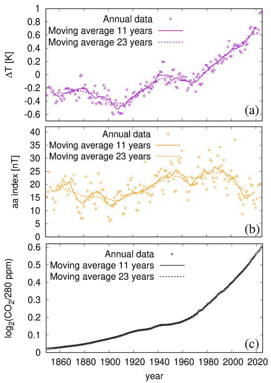
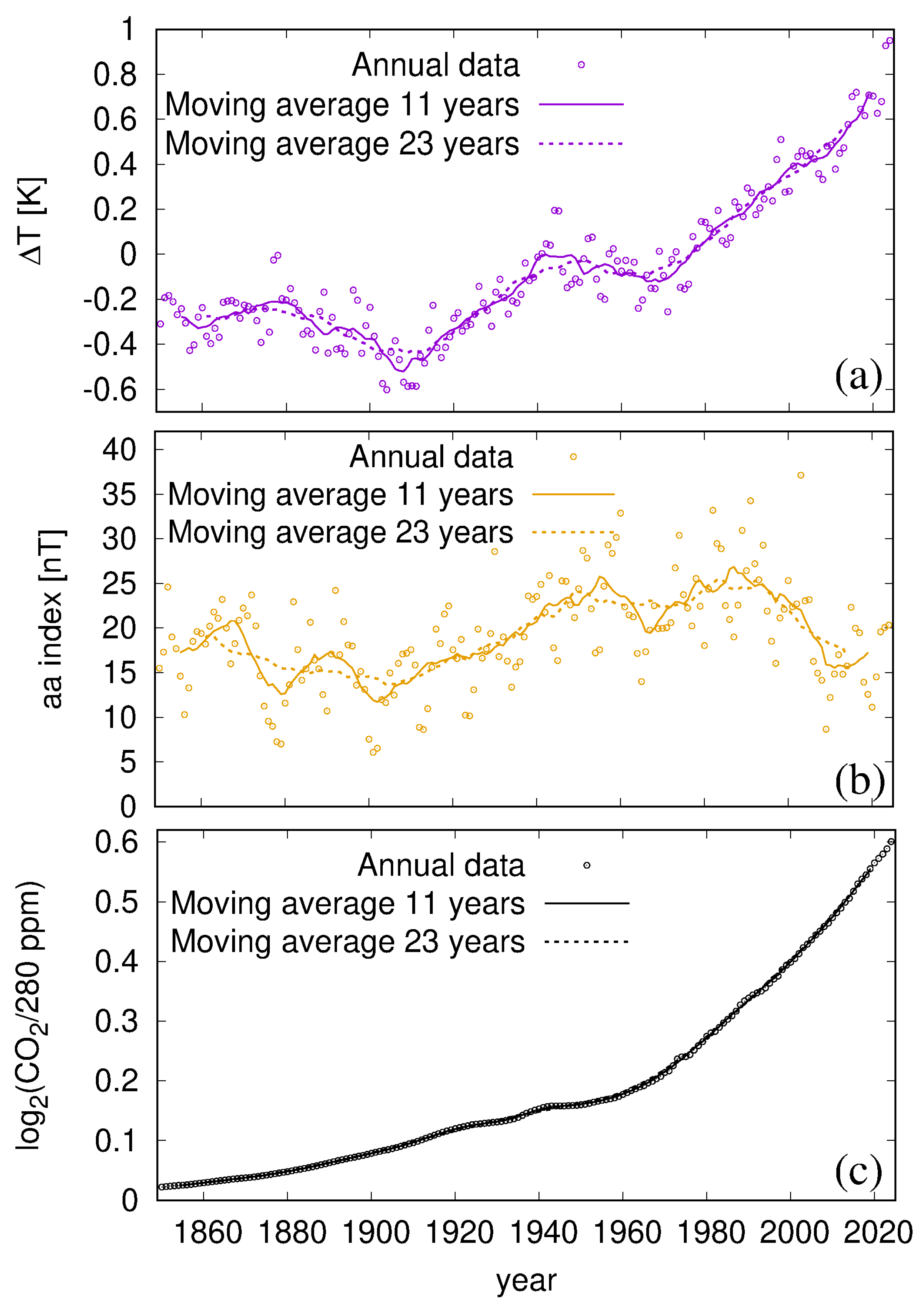
As for the temperature, the Hadley Centre Sea Surface Temperature (HadSST) data are used in the updated version HadSST.4.2.0.0, available from www.metoffice.gov.uk (accessed on 19 January 2026), which provides the sea surface temperature anomaly from 1850 until 2024, relative to the 1961–1990 average. The data are shown as open circles in Figure 1a, alongside two exemplary centred moving averages with moving average windows (MAWs) of 11 years (full line) and 23 years (dashed line). These curves exhibit a typical temporal structure: a slow decline between 1850 and 1905, a sharp rise between 1905 and 1940, and a gradual decline until 1970 followed by a sharp increase until 1998. Looking at the last decades, the first thing to notice is the “hiatus” between 1999 and 2014, followed by some strong El Niño events and finally the sharp increase to almost 1 K in 2023–2024.

Figure 1. Data on the HadSST sea surface temperature anomaly $\Delta T$ (a), the aa index (b), and ${\log }_2$ of the ratio of the CO₂ concentration to the reference value of 280 ppm (c). Centred moving averages with windows of 11 years (full lines) and 23 years (dashed lines) complement the annual data between 1850 and 2024. The sources of the data are described in the text.

The bulk of the aa index data, between 1868–2009, was obtained from the server https://www.ngdc.noaa.gov, accessed on 27 November 2025. As in [41], the early segment between 1844 and 1867 was taken from Nevanlinna and Kataja [56]. The latest segment, between 2010 and 2024, was obtained from www.geomag.bgs.ac.uk, accessed on 27 November 2025. All of the aa index data were averaged annually to provide a homogeneous dataset. Figure 1b shows the annual aa values together with their 11-year and 23-year moving averages. Interestingly, after 1990 the aa index declines while the temperature continues to increase.

The CO₂ data, the binary logarithm of which is shown in Figure 1c, were obtained from https://files.isimip.org and http://gml.noaa.gov/, accessed on 27 November 2025.

3. One Double and Two Single Regressions

As in [39] I will model the temperature (dependent variable) by using the ansatz

$$\Delta T^{\mathrm{model}}=w_{\mathrm{aa}}·\mathrm{aa}+w_{{\mathrm{CO}}_2}·{\log }_2({\mathrm{CO}}_2/280\mathrm{ppm})$$

with the respective weights $w_{\mathrm{aa}}$ and $w_{{\mathrm{CO}}_2}$ for the two independent variables $\mathrm{aa}$ and CO₂, comparing them with the measured data $\Delta T^{\mathrm{meas}}$.

In [39], it was shown that the outcome of the double regression is contingent on the final year of the used data. As for $w_{{\mathrm{CO}}_2}$, a value of 1.6 K was obtained when using 2018 as the end year, and 0.6 K when using 2008. The corresponding sensitivities $w_{\mathrm{aa}}$ were 0.017 K/nT and 0.032 K/nT, respectively.

Apart from potentially unconsidered factors, such as ENSO or the Hunga eruption, this sensitivity to end effects is also due to a high degree of collinearity between the two independent variables, aa and CO₂. This means that quite different combinations of the two weights can potentially produce very similar reconstruction qualities. In Figures 4–6 of [39] this collinearity was visible in the downward-directed ellipses that appear when plotting the fraction of variance unexplained (FVU) in the plane spanned by $w_{\mathrm{aa}}$ and $w_{{\mathrm{CO}}_2}$. Along the long axes of those ellipses the FVU changes only weakly.

In this picture, the strong end effect can be explained as follows: using a year too early means that the CO₂ did not have enough time to be reflected in the temperature curve, resulting in an underestimation of $w_{{\mathrm{CO}}_2}$. By contrast, for late end years, the weight may shift unduly from aa to CO₂, particularly if those final years are particularly hot, for example due to El Niño conditions or other factors.

In the following I will try to disentangle this problem in a systematic way. I start with the standard “statistically correct”, double regression, which is computed for all end years between 1950 and 2024. In parallel, two single regressions are carried out, with either aa or CO₂ as the sole independent variable. I commit this “statistical sin” very consciously (being fully aware of the criticism of [9] by [57]), to see how the results, and their $R^2$ values, compare with those of the “correct” double regression. This comparison will reveal some interesting insights into the dominance of each factor and how it changes over time.

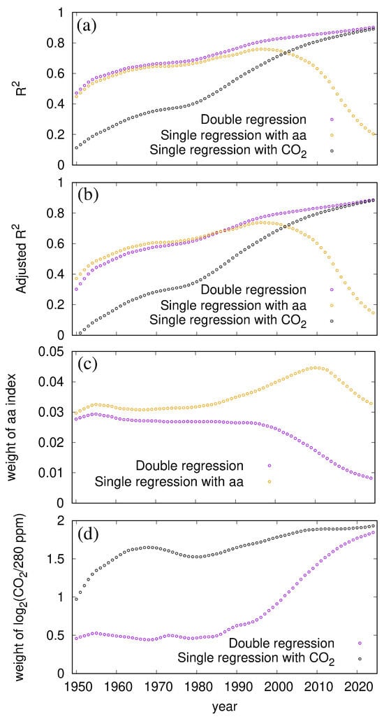
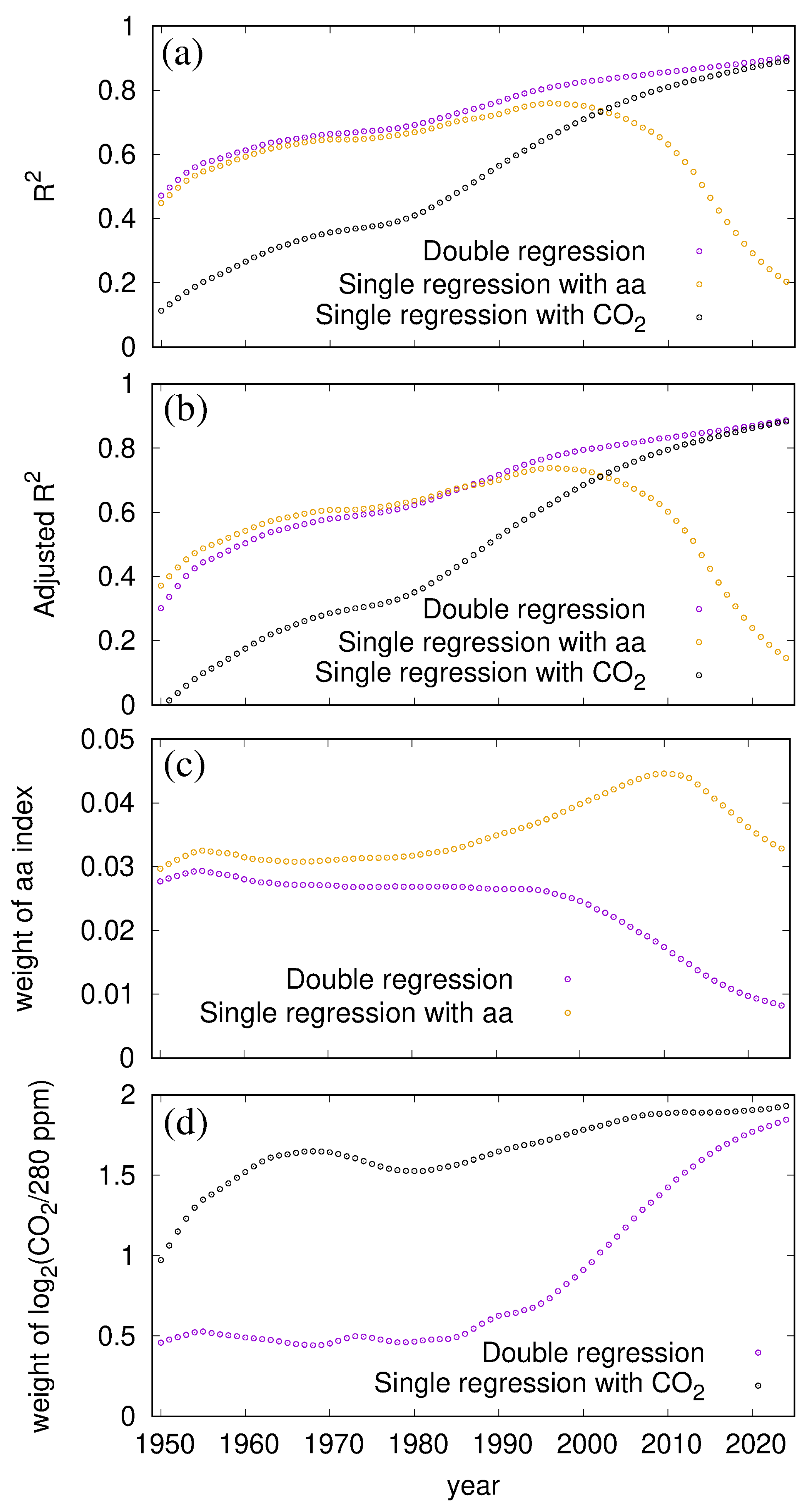
Let us start with an MAW of 11 years, which mainly “irons out” the effect of the Schwabe cycle of the solar dynamo on aa. Figure 2a shows the $R^2$ value for the double regression and the two single regressions on either aa or CO₂. Interestingly, until 1990, the two $R^2$ values for the double regression and the single one on aa are nearly identical, reaching values around 0.7 towards this year. Meanwhile, $R^2$ for the single regression on CO₂ is significantly smaller. Only from the year 2005 onward, the single-regression $R^2$ for CO₂ exceeds that for aa, and approaches that for the double regression in the 2020s. For those late years, we observe a drastic reduction in $R^2$ for the single regression on aa to a very low value of 0.2.

Figure 2. Regression results in dependence on the chosen end year for a moving average window ($\mathrm{MAW}$) of 11 years. (a) $R^2$ for the double regression and the two single regressions with either the aa index or the binary logarithm of CO₂ as the independent variable. (b) The same as (a), but for the adjusted version ${\overline{R}}^2$. (c) The resulting $w_{\mathrm{aa}}$ for the double regression and the single regression with aa as the only independent variable. (d) The resulting $w_{{\mathrm{CO}}_2}$ for the double regression and the single regression with CO₂ as the only independent variable.

Figure 2b shows the adjusted variant of $R^2$, coined ${\overline{R}}^2$, a useful indicator of a model’s true predictive power, which penalizes the addition of irrelevant variables and only increases if a new predictor significantly improves the model’s fit. In our special case, it can be computed as ${\overline{R}}^2=1-(1-R^2)(N_{\mathrm{y}}/\mathrm{MAW}-1)/(N_y/\mathrm{MAW}-1-p)$, where $N_{\mathrm{y}}$ is number of considered years and p the number of explanatory terms (i.e., two for the double and one for the single regression).

While its shape is not significantly different to that of the $R^2$ curve in Figure 2a, it is interesting to note that, until 1985, the ${\overline{R}}^2$ value for the single regression on aa is even higher than that for the double regression. Therefore, it is fair to say that, until this moment, the goodness of fitting $\Delta T$ by aa alone is higher than fitting it by aa and CO₂ jointly.

Figure 2c shows that the resulting weight of aa until this moment is relatively constant (around 0.03 K/nT), with only a minor difference between the double and the single regression. Later, however, the value from the double regression drops to 0.01 K/nT, while the value from the single regression is no longer meaningful in view of the drastically falling $R^2$ value. In contrast, the double regression value for $w_{{\mathrm{CO}}_2}$ remains low at 0.5 K until 1990, after which it increases steeply to reach 1.8 K by the year 2024.

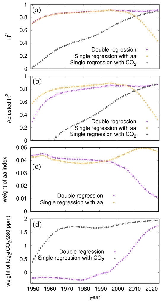
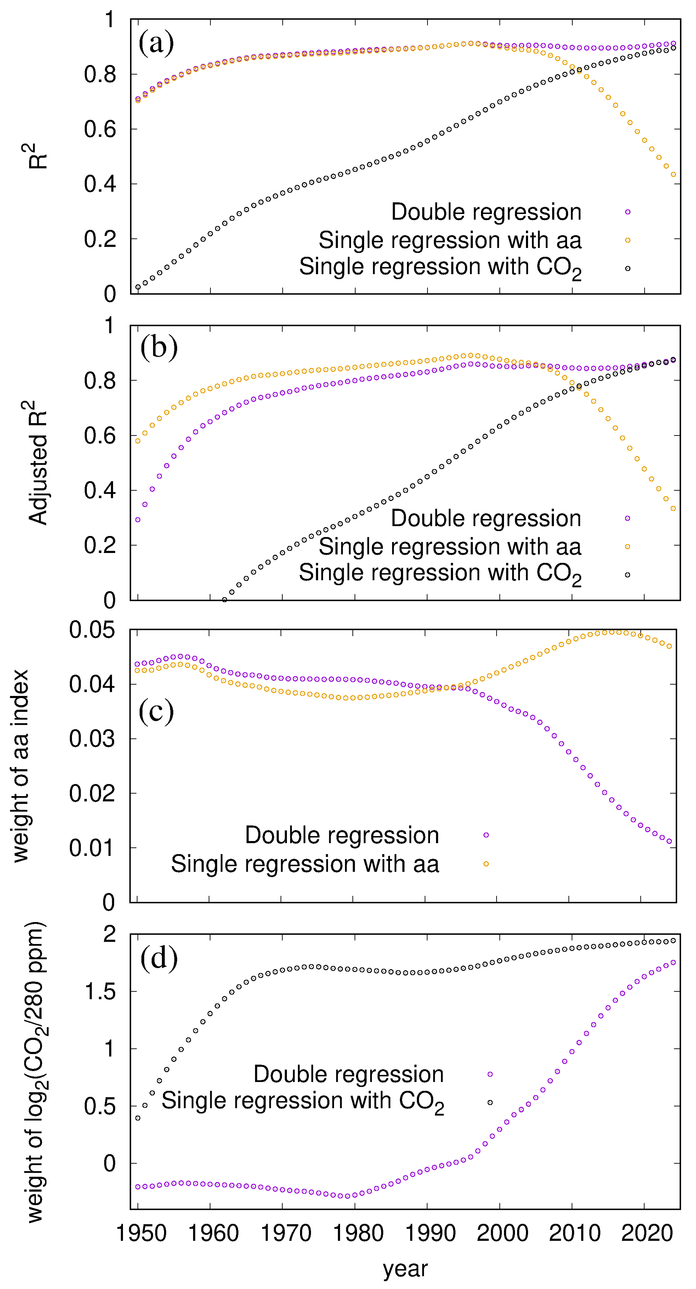
Figure 3 shows the qualitatively similar behavior when an MAW of 23 years is chosen. Here, the ${\overline{R}}^2$ for the single regression on aa remains higher than that for the double regression even until the year 2005. Again one could argue that, until this year, including CO₂ would only worsen the goodness of fit. For this MAW, the long-term result for w_aa is around 0.04 K/nT, while it drops to 0.01 K/nT for the final year 2024. Accordingly, w_CO2 remains close to zero until 2000, after which it increases steeply to reach 1.7 by 2024.

Figure 3. The same as Figure 2, but with an MAW of 23 years. Note that in (b) the adjusted version ${\overline{R}}^2$ formally acquires, for early years, negative values.

Clearly, there is a problem here. On one hand, until the end of the 20th century, $\Delta T$ turns out to be more or less perfectly predicted by aa alone, resulting in a quite stable aa sensitivity of approximately 0.04 K/nT (if we chose an MAW of 23 years for which the ${\overline{R}}^2$ values of approximately 0.9 are higher than those for 11 years). On the other hand, the steep temperature increase over the past decades requires not only an increasing share of CO₂ (which is well understandable in view of its steep increase; see Figure 1c), but also a dramatic decrease of $w_{\mathrm{aa}}$ which is much harder to explain. In our view, the only explanation is that some part of the $\Delta T$ increase over the last years is due to some other effects (beyond CO₂), like ENSO or the Hunga volcano, which are not properly included in our simple model.

Therefore, we must either accept an unreasonably large reduction in the aa sensitivity over the last two decades (compared with its long-term stable average), or attribute some of the recent steep warming to factors other than CO₂ or solar activity.

The second approach will be tentatively pursued in the following (its correctness will ultimately be judged by the temperature development over the next years). Specifically, the long-term result of about 0.03–0.05 K/nT for $w_{\mathrm{aa}}$ will also be used for the later times, for which the double regression would predict a much reduced value. Having thus fixed $w_{\mathrm{aa}}$, one is left with another single regression on CO₂, but this time of a modified $\Delta T$ that is reduced by the aa contribution weighted by the $w_{\mathrm{aa}}$ derived beforehand.

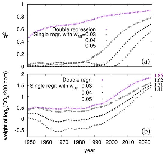
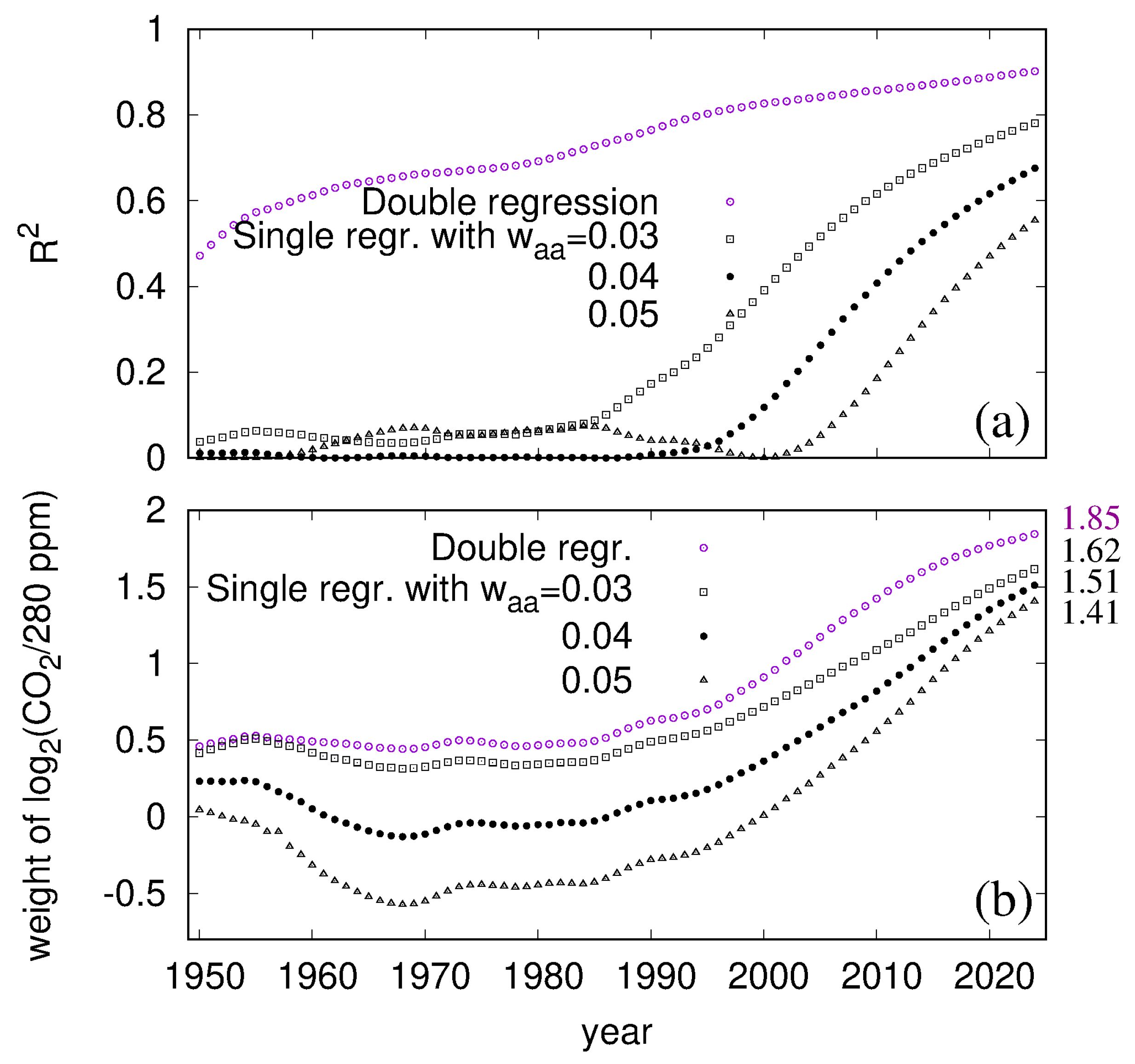
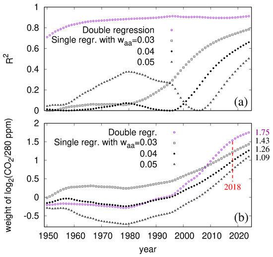
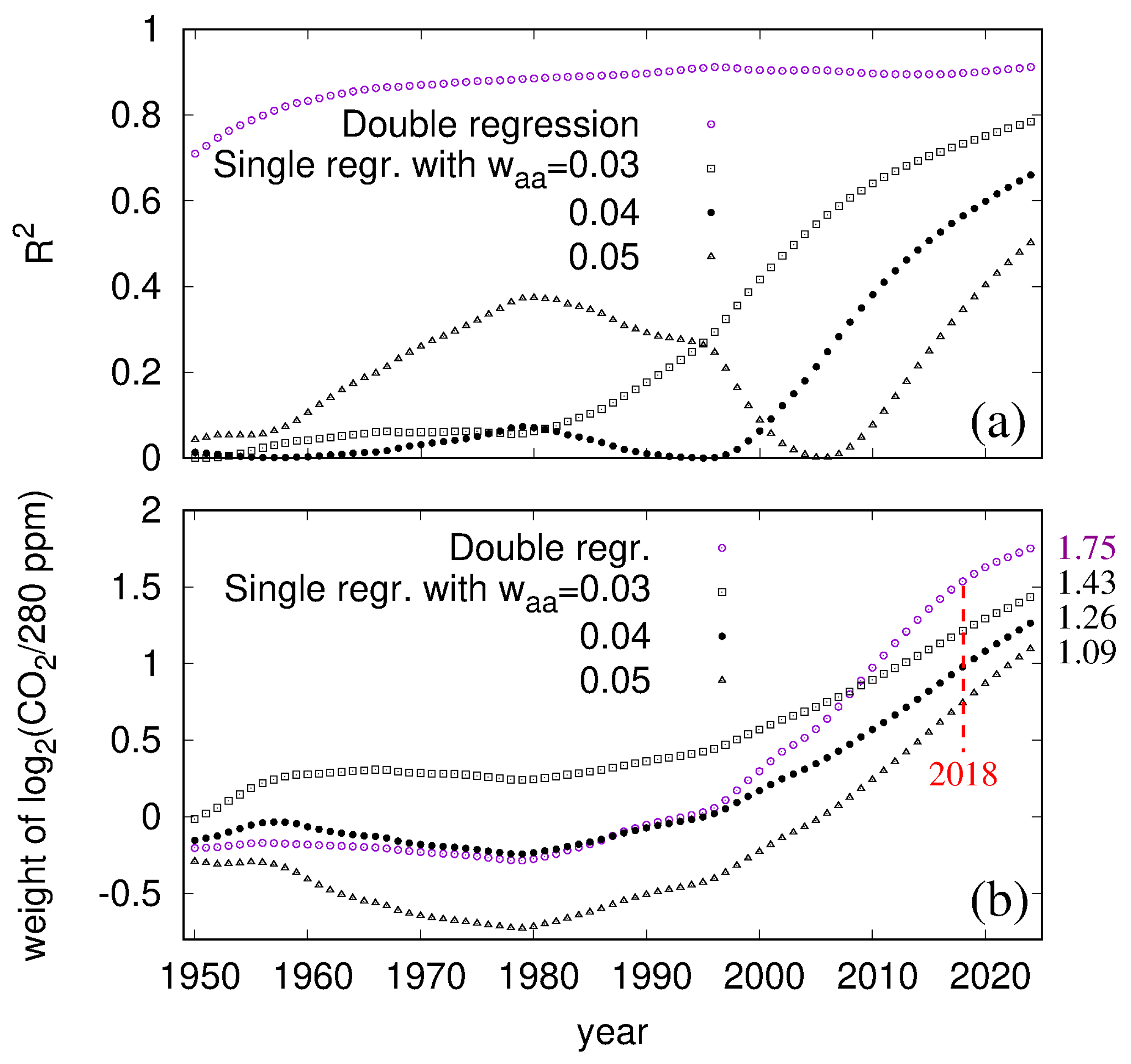
This procedure is illustrated in Figure 4 (for an MAW of 11 years) and Figure 5 (for an MAW of 23 years). Here the violet curves for $R^2$ (a) and $w_{{\mathrm{CO}}_2}$ (b) correspond, respectively, to those from panels (a) and (d) of Figure 2 and Figure 3. The black curves, however, result when first subtracting from $\Delta T$ an aa contribution weighted by a fixed $w_{\mathrm{aa}}$. For the latter we chose a certain variety, ranging from 0.03 K/nT (according to Figure 2c), via 0.04 K/nT (according to Figure 3c) to 0.05 K/nT (the uppermost value in Figure 3c).

Figure 4. Regression results dependent on the chosen end year for a moving average window ($\mathrm{MAW}$) of 11 years. (a) $R^2$ for the double regression (as in Figure 2a) and the three single regressions on the binary logarithm of CO₂ as the independent variable, when subtracting beforehand from $\Delta T$ the aa contribution weighted with three different values of $w_{\mathrm{aa}}$ (0.03 K/nT, 0.04 K/nT, and 0.05 K/nT). (b) The resulting $w_{{\mathrm{CO}}_2}$ for the double regression and the three single regressions.

Figure 5. Same as Figure 4, but for an MAW of 23 years.

Note that constraining $w_{\mathrm{aa}}$ beforehand has a non-trivial impact on the subsequent single regression on CO₂. On one hand, it tends to require less of $w_{{\mathrm{CO}}_2}$ since a larger proportion of the increase between 1850 and 2000 has already been attributed to aa. On the other hand, for the late interval, starting from 1990, even more $w_{{\mathrm{CO}}_2}$ is required to compensate for the strongly negative aa contribution due to the steep aa decline during those years. Obviously, the combined effect of these two tendencies leads to a moderate reduction in the resulting $w_{{\mathrm{CO}}_2}$ compared to the double regression.

The resulting $w_{{\mathrm{CO}}_2}$ values in the final year, 2024, are indicated on the right-hand ordinate axis of Figure 4b (for an MAW of 11 years) and Figure 5b (for an MAW of 23 years). The latter values, 1.09–1.43 K are situated in the upper half of the 0.6–1.6 K range that was predicted in [39]. This upward trend is mostly due to the high temperatures that have been recorded over the past six years. Had we carried out the same procedure based on the previous dataset (up to 2018), we would have obtained a range of 0.8–1.2 K (see the red line in Figure 5b), which lies slightly below the middle of the 0.6–1.6 K interval.

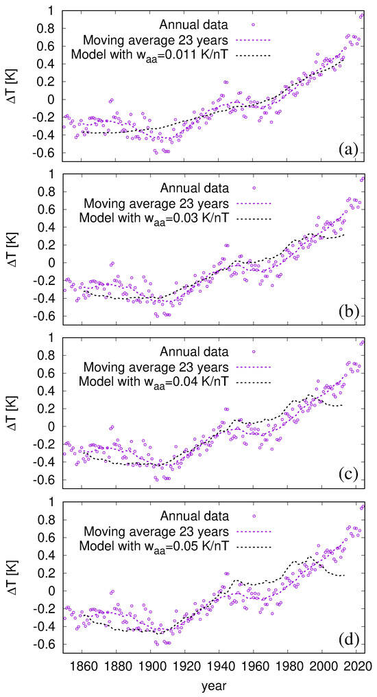
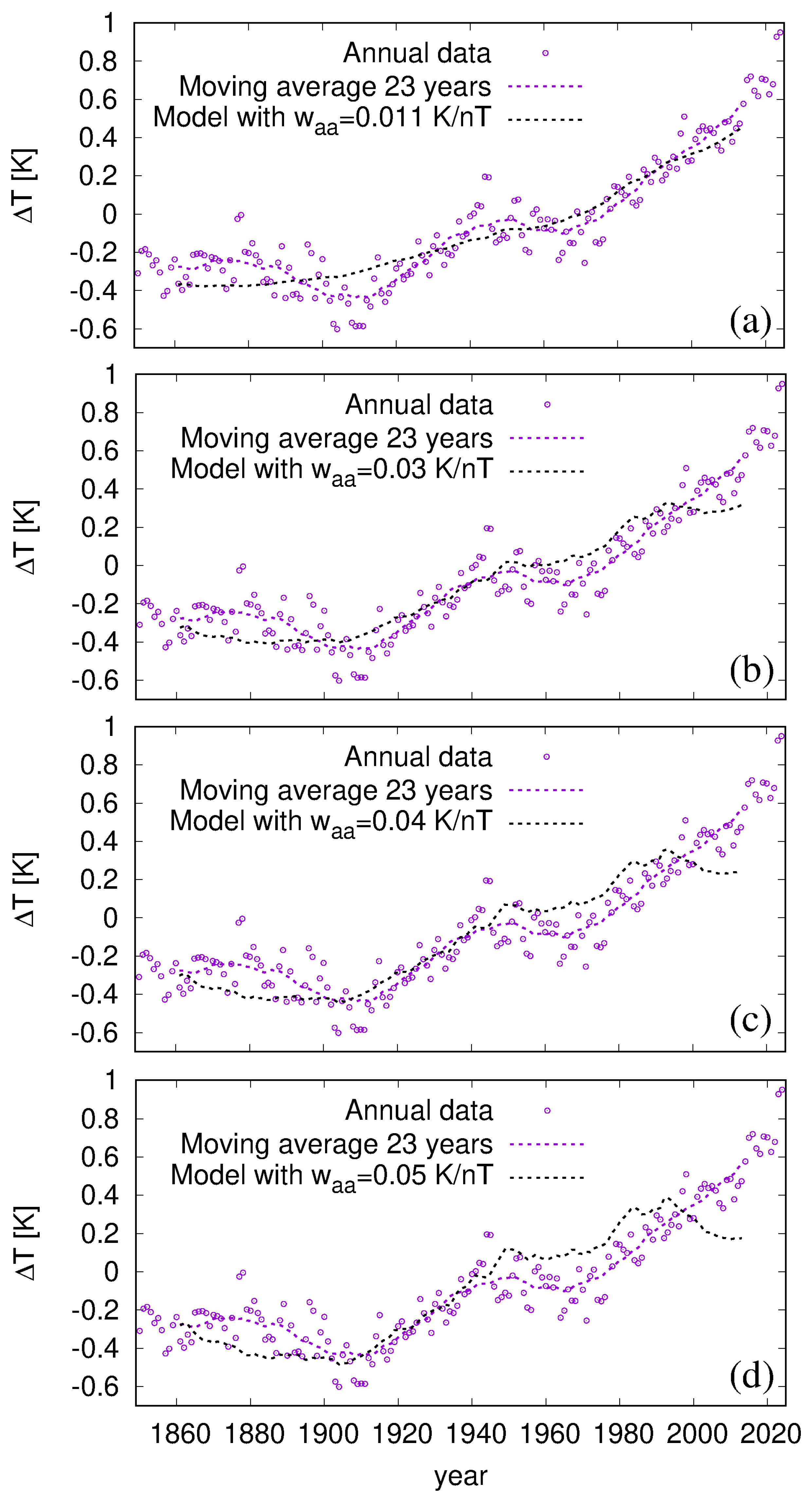
Figure 6 focuses on the MAW of 23 years and illustrates how the resulting combinations of $w_{{\mathrm{CO}}_2}$ and $w_{\mathrm{aa}}$ play out in comparison with the original $\Delta T$ data. Figure 6a shows a reasonable behavior in recent years when the results of the “correct” double regression are chosen, i.e., $w_{\mathrm{aa}}=0.011$ K/nT and $w_{{\mathrm{CO}}_2}=1.75$ K. Obviously, this comes at the cost of barely reflecting the temperature variability between 1850 and the end of the 20th century. This variability is better reflected when accepting for $w_{\mathrm{aa}}$ the long-term outcomes of 0.03 K/nT (b), 0.04 K/nT (c) or 0.05 K/nT (d), together with the corresponding $w_{{\mathrm{CO}}_2}$ values of 1.43 K, 1.26 K and 1.09 K. However, the temperature of the latest years, as might be expected, is becoming less and less accurately represented.

Figure 6. Data of $\Delta T$ and their average with an MAW of 23 years as in Figure 1a, together with reconstructions with different sensitivity parameter combinations. (a) $w_{\mathrm{aa}}=0.011$ K/nT and $w_{{\mathrm{CO}}_2}=1.75$ K, resulting from the double regression until the end year 2024. (b) $w_{\mathrm{aa}}=0.03$ K/nT and $w_{{\mathrm{CO}}_2}=1.43$ K. (c) $w_{\mathrm{aa}}=0.04$ K/nT and $w_{{\mathrm{CO}}_2}=1.26$ K. (d) $w_{\mathrm{aa}}=0.05$ K/nT and $w_{{\mathrm{CO}}_2}=1.09$ K.

4. Predictions

In the preceding section, regression analyses of data from the past 175 years were used to derive a range of plausible combinations of the respective sensitivities on the aa index and the binary logarithm of CO₂. In the following, I will employ these results to forecast the global mean temperature until 2100. While forecasts up to this year are already highly uncertain, any prediction beyond this point would be subject to enormous imponderables with regard to both the future dominant energy technologies (and the resulting emissions) and the variability of the solar dynamo.

4.1. Predicting CO₂

Let us begin by discussing the most plausible evolution of the atmospheric CO₂ concentration $C\left(t\right)$ until 2100. This requires estimates of the time-dependent sources (emissions) $E\left(t\right)$ and the sinks $S\left(t\right)$. Quite generally, $C\left(t\right)$ is governed by the following rate equation:

$${\displaystyle \frac{dC\left(t\right)}{dt}}=E\left(t\right)+S\left(t\right).$$

(1)

Regarding the source term $E\left(t\right)$, I will rely solely on the International Energy Agency’s (IEA) recent forecasts until 2050 [50], rather than considering the wide variety of representative concentration pathways (RCPs) or shared socioeconomic pathways (SSPs). The most reasonable estimates for the current and stated policy scenarios until 2050 were shown in Figures 3.3 and 4.3 of [50]. Remarkably, under the current policies, the emission is expected to remain almost unchanged at around 38 Gt/yr. In a more “optimistic” scenario, the implementation of the stated policies would result in a decrease to 30 Gt/yr. Considering the generally increasing energy demand in parallel with the growing proportion of renewable and nuclear energy, it seems most plausible to assume a relatively constant emission scenario of 40 Gt/yr even until the year 2100. Such an IEA-based scenario is at least much more realistic than the so-called “business as usual” RCP8.5 scenario, which has been thoroughly debunked [58,59]. However, I will also examine values that are slightly lower (30 Gt/yr) or slightly higher (50 Gt/yr), thereby covering a certain plausible range.

Now let us consider the sink term $S\left(t\right)$. It is well known that at present approximately half of the current emissions are absorbed by the oceans and land plants [51], and that this absorption increases as the actual CO₂ concentration diverges further from its pre-industrial equilibrium value $C_{\mathrm{eq}}=280$ ppm. However, the details of this concentration dependence are not well known. Corresponding considerations typically fall under the notion of carbon-concentration feedback. While these feedbacks were initially discussed [60,61] in terms of time-integrated flux changes due to an increase in $C\left(t\right)$ (and corresponding changes due to a temperature increase, a minor effect that is ignored here), the instantaneous version of Boer and Arora [62] appears more understandable and useful. These authors set out from the premise that $S\left(t\right)$ can be expanded in a Taylor series in $C\left(t\right)-C_{\mathrm{eq}}$, i.e., around the equilibrium value $C_{\mathrm{eq}}=280$ ppm, beginning with the linear term. As in [62], here we use the ansatz $S\left(t\right)=B\left(t\right)(C\left(t\right)-C_{\mathrm{eq}})$. Although $B\left(t\right)$ can be considered constant for small values of $C\left(t\right)-C_{\mathrm{eq}}$, it may deviate from this for larger values, which would correspond to terms higher than linear in the Taylor expansion. According to Figure 4 of [62], this deviation depends, in turn, on the emission scenario. While for the unrealistic scenario RCP8.5, $B\left(t\right)$ remains rather constant at approximately −0.04 GtC/(yr ppm), it weakens for the RCP4.5 scenario to values of −0.03 GtC/(yr ppm) or even −0.02 GtC/(yr ppm). Later on, we will consider such modified values of $B\left(t\right)$ as alternative scenarios.

For now, however, we will stick to the constant term and set it to $B=-0.02$ yr⁻¹. This value was chosen based on recent empirical estimations [51,52]. Yet, it is also compatible with the above value of −0.04 GtC/(yr ppm) [62] when considering the equivalence 1 ppm $\widehat{=}$ 2.124 GtC $\widehat{=}$ 7.782 GtCO₂.

Assuming a constant emission term E and a constant value of B, the resulting simple differential equation

$${\displaystyle \frac{dC\left(t\right)}{dt}}=E+B(C\left(t\right)-C_{\mathrm{eq}})$$

(2)

acquires the analytical solution

$$\begin{array}{c}\hfill C\left(t\right)=K\exp \left(B(t-t_0)\right)-(E/B-C_{\mathrm{eq}}),\end{array}$$

(3)

with the integration constant $K=C\left(t_0\right)+(E/B-C_{\mathrm{eq}})$. In the following, $t_0$ will be set to 2024, with $C(t_0=2024)=424.6$ ppm.

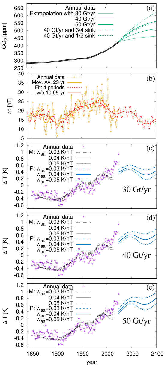
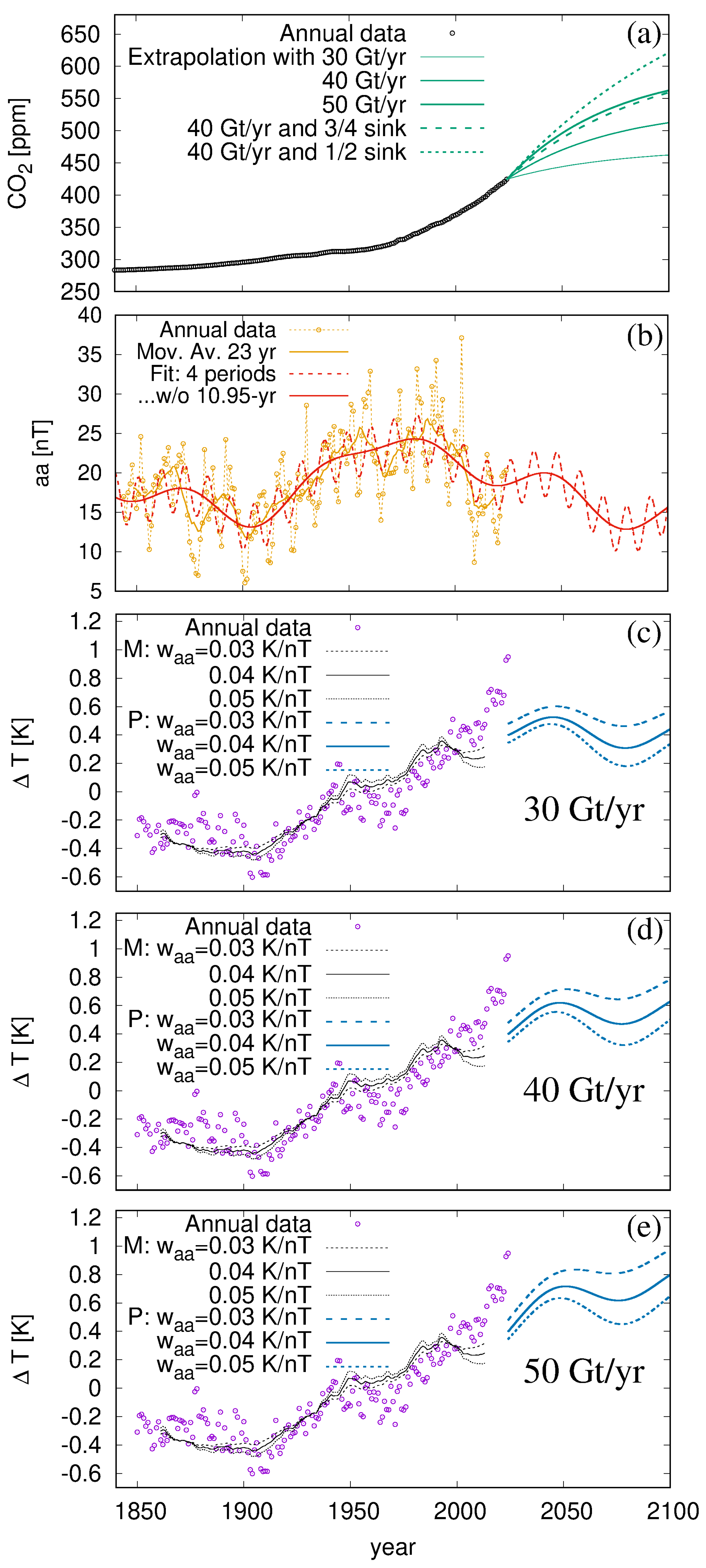
In Figure 7a, the solid green lines show the solutions when setting, in Equation (3), E to either 3.85 ppm/yr $\widehat{=}$ 30 Gt/yr, 5.14 ppm/yr $\widehat{=}$ 40 Gt/yr or 6.43 ppm/yr $\widehat{=}$ 50 Gt/yr, always choosing $B=0.02$ yr⁻¹. As we can see, in the year 2100 the curves terminate at values between 460 ppm and 560 ppm, nearly approaching the respective equilibrium values 473 ppm, 537 ppm and 601 ppm that would result (when setting the r.h.s. of Equation (2) to zero) for annual emissions of 30, 40, and 50 Gt, respectively. Only for the case of 40 Gt/yr two further curves are added, corresponding to the absorption coefficient B being reduced by a factor 3/4 (dashed line) or 1/2 (dotted line), as inspired by Figure 4 of [62]. As can be seen, the curve for 40 Gt/yr with B reduced to 3/4 is very close to the curve for 50 Gt/yr with the full B. Hence, later on I will focus only on the three different emission scenarios, keeping B always fixed at $0.02$ yr⁻¹.

Figure 7. Data until 2024, and forecasts until 2100. (a) CO₂ content according to Equation (3) with sink parameter $B=-0.02$ yr⁻¹ and three annual emission values (30, 40, and 50 Gt), and with two reduced sink terms (only for 40 Gt). (b) Best fit of the aa index by three dominant periods (and a Schwabe-type period of 10.95 years), according to the synchronization model of [32], and its extrapolation until 2100. (c) Temperature data, their modelings (M) according to Figure 6b–d, and predictions (P) for three parameter combinations of $w_{\mathrm{aa}}$ (0.03 K/nT, 0.04 K/nT, and 0.05 K/nT) and $w_{{\mathrm{CO}}_2}$ (1.43 K, 1.26 K and 1.09 K). For the predictions, annual emissions of 30 Gt are assumed. (d) Same as (c), but for 40 Gt. (e) Same as (c), but for 50 Gt.

4.2. Predicting the Solar Dynamo

Having explained the choice of the most plausible CO₂ scenarios until 2100, I now turn to forecasting the aa index. It is well known that the aa index (as well as the sunspot number, with which aa is strongly correlated [63]), is governed by the solar dynamo. Clearly, any forecast of the aa index hinges on predicting the solar dynamo.

As in [39], the aa forecast is based on the synchronized solar dynamo model, which we have corroborated over the last decade [32,49,64,65,66,67,68,69,70,71,72,73]. While this model had been the subject of controversy until recently [74,75], its latest embodiment [32,49,73], which is based on the tidal excitation of magneto-Rossby waves at the solar tachocline, shows remarkable agreement with observations. Firstly, the model provides an extremely accurate representation of the period of the Quasi-Biennial Oscillation (QBO), viz., 1.723 years in the model versus 1.724 years based on observations of ground-level enhancement events [49,76]. Secondly, when also incorporating the spin–orbit coupling effect due to the rosette-shaped motion of the sun around the solar system’s barycenter, the model yields dominant spectral peaks that are in stunning agreement with those of sediment data from Lake Lisan (see Figure 9 in [32]). The latter agreement also points to a significant top-down effect whereby stratospheric–tropospheric coupling influences the trajectories of North Atlantic cyclones [33], which presumably are responsible for the precipitation rates in the Lake Lisan region [31].

Given the model’s ability to explain the three dominant periods, it is recommended that the resulting values for the Suess-de Vries cycle (193 years) and the two Gleissberg-type cycles (57 and 90 years) be employed for fitting the aa index data. To mitigate any end effects, a Schwabe cycle was added as a fourth period. Instead of the theoretical value of 11.07 years resulting from our model [32], the slightly modified value of 10.95 years is used, according to the empirical analysis of [77].

Figure 7b shows the resulting fit of the aa index data, represented by the dashed red line. The long-term part (full red line), with the 10.95 yr contribution subtracted, is then extrapolated until 2100. Evidently, the interplay of one Suess-de Vries and two Gleissberg cycles predicts a shallow maximum around 2045 and a minimum around 2080 which is as deep as the so-called “Gleissberg minimum” around 1900 [78].

4.3. Predicting the Temperature

Using these CO₂ and aa index predictions, I will now attempt to forecast the global mean temperature until 2100. To achieve this, I first assume (full blue line in Figure 7d) a conservative emission scenario with 40 Gt/yr, an aa sensitivity of 0.04 K/nT and a corresponding CO₂ sensitivity of 1.26 K. While in terms of the underlying CO₂ history this combination is similar to the middle scenario shown as the green line in Figure 9d of [39], its higher aa sensitivity leads to a more oscillatory behavior of the temperature curve. Following a slight increase until 2050 and a modest decline until 2080, the temperature reaches 0.6 K in 2100. The dashed and dotted blue lines added in Figure 7d refer to decreased (0.03 K/nT) and increased (0.05 K/nT) values of $w_{\mathrm{aa}}$, combined with the respective values of 1.43 K and 1.09 K for $w_{{\mathrm{CO}}_2}$. Note that the little “jump” between the black and the blue curves is due to the fact that the former originate from applying the respective sensitivities to the measured aa and CO₂ data while the latter rely on an extrapolation of the three-period fit to aa (and a fixed emission rate of CO₂). In either case, the respective end and start points are clearly at odds with the actual data. Meanwhile, however, a significant portion of this discrepancy has been resolved by the temperature decline in 2025 and early 2026, marking a substantial drop from the extreme values recorded in 2023/2024. It remains to be seen whether the gap between the moderately high values of 2015–2022 and the forecast (blue curves) will close in the years to come.

Figure 7c,e shows the corresponding curves for (hypothetical) reductions or enhancements of the annual emissions to 30 Gt or 50 Gt, respectively. Roughly speaking, these emission changes lead to a decrease or increase in the final temperature of around 0.2 K.

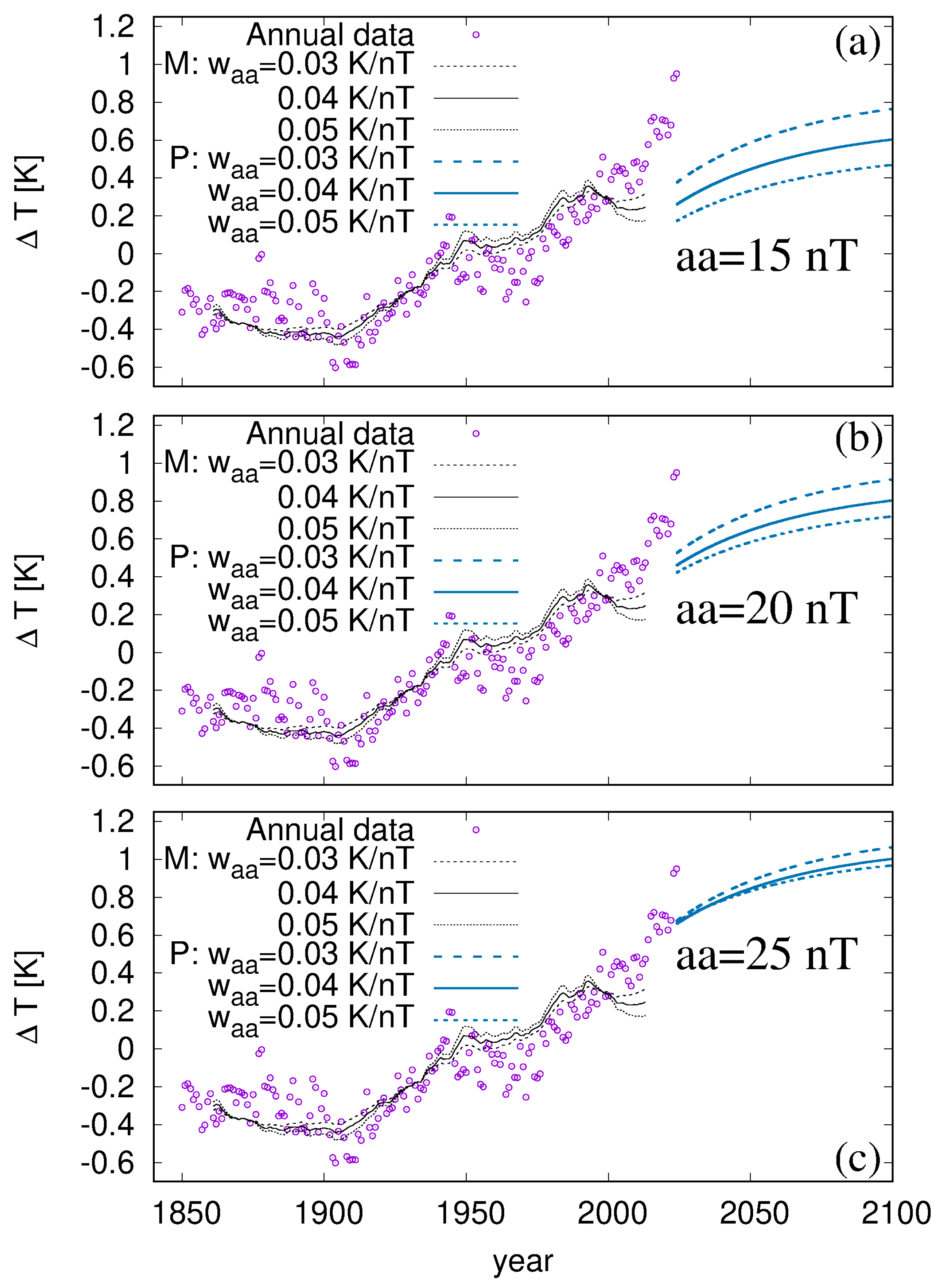
As the aa index prediction appears to be the riskiest, Figure A1 in Appendix A also shows (only for annual emissions of 40 Gt) the forecasts assuming three constant aa values of 15, 20 and 25 nT, which cover the typical aa range of the last 180 years. Rather than exhibiting the typical wiggly behavior with a minimum around 2080, these curves show a monotonic, albeit flattening, increase until 2100. For the highest aa value of 25 nT, this terminates at 0.3 K above the maximum value in Figure 7d.

5. Summary and Discussion

The aim of this work was to update and refine the previous estimate [39] of the influence of solar activity variations and CO₂ on the terrestrial climate, and to improve the global temperature prediction until the end of this century. Having supplemented the underlying dataset with information from the last six years (2019–2024), an attempt was made to narrow the broad range of climate sensitivities (on both the aa index and CO₂ doubling) that had resulted from the double regression in [39]. For two different lengths of the moving average window I have compared the time dependence of the goodness of fit for the “statistically correct” double regression with those for single regressions on aa or CO₂, respectively. It was shown that, until the end of the 20th century, the $R^2$ value of the double regression was almost identical to that obtained using the aa index alone. This indicates that the sun’s impact on climate was the dominant factor up to that point. This result not only contrasts with the original idea of [8] and the subsequent claim of [6] that “(t)he partial correlation with CO₂ indeed dominates over that of solar irradiance for the most recent 200-year interval”, but it also contradicts the more Solomon-like judgment of [79] that “since roughly 1970 the solar influence on climate…cannot have been dominant”. When assessing the adjusted ${\overline{R}}^2$ until 1985 (using an MAW of 11 years) or 2005 (using an MAW of 23 years), the single regression on aa alone yields higher values than the double regression. It was only since the beginning of the 21st century that the contribution of CO₂ has become noticeable and prominent.

Given the remarkable stability of the aa sensitivity resulting from the double and single regressions over the long period between 1950 and 1990, the outcome of around 0.04 K/nT was considered plausible for subsequent decades as well. Based on this reasoning, the CO₂ sensitivity was recalculated by first subtracting the aa contribution (weighted by the aa sensitivity obtained beforehand) from the observed $\Delta T$ and then regressing the remaining $\Delta T$ on CO₂. Although this procedure may appear to be a “statistical sin”, I consider its outcome to be better justified than that of a “correct”, albeit somewhat naive double regression. That way, the CO₂ sensitivity was narrowed down from the ample range of 0.6–1.6 K derived in [39] to 1.1–1.4 K. The alternative double regression would not only have resulted in a moderately enhanced CO₂ sensitivity value of 1.74 K, but also in a dramatically reduced aa sensitivity of 0.011 K/nT. Faced with the choice of either accepting an unreasonably huge reduction in the aa sensitivity over the last two decades (compared with its stable long-term average) or attributing some of the recent steep warming to factors other than CO₂ or the sun, I opted for the latter. While the recent temperature decline until the end of 2025 bodes well for the correctness of this approach, only future data will provide a definite answer. It goes without saying that the method could be improved by including further factors, such as ENSO and volcanic activity, including the barely quantified climatic effects resulting from dramatic events such as the Hunga eruption. Moreover, a great deal of future work will be required to corroborate in detail the climate-relevant mechanisms mentioned in the introduction (TSI, ultraviolet radiation and stratospheric–tropospheric coupling, cosmic rays, etc.), for which the aa index was used as a convenient proxy here.

In the parlance of global circulation models, the derived CO₂ sensitivity should be considered a type of TCR rather than ECS. The obtained range of 1.1–1.4 K lies at the lower end of the values published by the IPCC (1.2–2.4 K) [2], but corresponds reasonably with those of Lewis and Curry [80], and Scafetta [37]. As the values of $\Delta T$ in the final years of the period under consideration were particularly high, it seems likely that including data from the following years will result in a slight decrease of the values. Although it is highly unlikely, we cannot rule out the possibility that the recent rise in temperature is largely due to CO₂. In this case, however, the aa sensitivity would have had to have decreased significantly in recent decades for some unknown reasons.

In the second part of the paper, I have made another attempt to forecast the global temperature until the end of the century based on the sharpened ranges of the two climate sensitivities. In addition to that reduction, I also limited the potential CO₂ history to three variants. All of them rely on constant annual emissions (30, 40 or 50 Gt) over the next few decades (see [50]), and on a simple linear sink model, which I consider most plausible in view of the results of [51,52].

As for the prediction of the aa index, the variety of models of [39] was restricted to a single one comprising the three dominant periods (one Suess-de Vries and two Gleissberg cycles) according to our synchronized solar dynamo model. Although this may seem overly specific, the use of this model was encouraged by the fact that its resulting spectrum corresponds remarkably well with climate-related sediment data from Lake Lisan [31,32].

The combined forecast model yields, for the terminal year 2100, a rather benign temperature increase of approximately 0.6 K, compared to the standard HadSST data reference period (1961–1990). For each emission scenario, the temperature spread between the considered aa sensitivity models was approximately 0.3 K, whereas the corresponding spread between different emission scenarios was around 0.4 K.

Only for the most “pessimistic” parameter combination (assuming high annual emissions of 50 Gt, a low aa sensitivity of 0.03 K/nT, and an accordingly high CO₂ sensitivity of 1.43 K) I obtained a temperature rise to slightly more than 1 K. This essentially corresponds to the extraordinarily high value measured in 2024. For all other parameter combinations we would stay below this value.

When compared with the minimum temperature in the dataset (approximately −0.4 K around 1900), the increase is no greater than 1.5 K. Regardless of the actual relevance of the politically pursued 1.5-degree target, there seems to be no danger of exceeding it if we assume that emissions will remain at current levels. This message would barely change if we replaced the somewhat risky forecast of the aa index with the assumption that it would remain constant at values typical of the last 180 years.

6. Conclusions and Outlook

All forecasts were deliberately restricted until 2100, primarily because of the significant uncertainty surrounding the CO₂ emission scenarios. While neither a huge increase in emission values (as in the former scenario A2 [60] or the recent scenario RCP8.5 [62]), nor a dramatic decrease to an illusory “net zero” regime appears very likely, it would be preposterous to prophesy the energy production landscape in one hundred years’ time.

A similar caveat applies to solar activity. While the dominant periods used here are typical of a regular solar dynamo behavior, we cannot rule out the occurrence of a new grand solar minimum (i.e., the next Bond event) in the centuries to come. Transitions between regular and chaotic regimes of the solar dynamo, termed supermodulation in [81], appear to be non-deterministic [70], although the Bray–Hallstadt cycle (approximately 2300 years) may also play a certain role here [82].

Finally, we should always bear in mind that we are amidst the decline phase of the glacial cycle which is governed by changing insolation conditions, dominated by the Milankovitch cycles. Interestingly, glaciation always occurred when the nutation angle of the Earth decreased below 23°, though deglaciation was sometimes missed when it increased above 23°. This effect was recently discussed by Vinós [83], who also employed it to solve the longstanding 100,000-year problem.

In any case, it is only when considering the ECS, and its century-long relaxation mechanism, that those long-term effects might acquire any relevance. Even assuming annual CO₂ emissions of 30, 40 or 50 Gt, the predicted benign temperature rise until 2100 gives us ample time to develop cost-efficient alternatives to fossil fuels that will not result in an unnecessary reduction in living standards.

References

- Charney, J.; Arakawa, A.; Baker, D.J.; Bolin, B.; Dickinson, R.E.; Goody, R.M.; Leith, C.E.; Stommel, H.M.; Wunsch, C.I. Carbon Dioxide and Climate: A Scientific Assessment; National Academy of Sciences Press: Washington, DC, USA, 1979. [Google Scholar]
- IPCC. Climate Change 2021: The Physical Science Basis. Contribution of Working Group I to the Sixth Assessment Report of the Intergovernmental Panel on Climate Change; Masson-Delmotte, V., Zhai, P., Pirani, A., Connors, S.L., Péan, C., Berger, S., Caud, N., Chen, Y., Goldfarb, L., Gomis, M.I., et al., Eds.; Cambridge University Press: Cambridge, UK, 2021. [Google Scholar]
- Knutti, R.; Rugenstein, M.A.A.; Hegerl, G.C. Beyond equilibrium climate sensitivity. Nat. Geosci. 2017, 10, 727–736. [Google Scholar] [CrossRef] [Scilit]
- Bond, G.; Kromer, B.; Beer, J.; Muscheler, R.; Evans, M.N.; Showers, W.; Hoffmann, S.; Lotti-Bond, R.; Hajdas, I.; Bonani, G. Persistent solar influence on North Atlantic climate during the Holocene. Science 2001, 294, 2130–2136. [Google Scholar] [CrossRef] [Scilit]
- Lean, J.; Beer, J.; Bradley, R. Reconstruction of solar irradiance since 1610: Implications for climate change. Geophys. Res. Lett. 1995, 22, 3195–3198. [Google Scholar] [CrossRef] [Scilit]
- Mann, M.E.; Bradley, R.S.; Hughes, M.K. Global-scale temperature patterns and climate forcing over the past six centuries. Nature 1998, 392, 779–787. [Google Scholar] [CrossRef] [Scilit]
- McIntyre, S.; McKitrick, R. Hockey sticks, principal components, and spurious significance. J. Geophys. Res. 2005, 32, L03710. [Google Scholar] [CrossRef] [Scilit]
- Callendar, G.S. The artificial production of carbon dioxide and its influence on temperature. Q. J. R. Meteorol. Soc. 1938, 64, 223–240. [Google Scholar] [CrossRef] [Scilit]
- Connolly, R.; Soon, W.; Connolly, M.; Baliunas, S.; Berglund, J.; Butler, C.J.; Cionco, R.G.; Elias, A.G.; Fedorov, V.M.; Harde, H.; et al. How much has the Sun influenced Northern hemisphere temperature trends. An ongoing debate. Res. Astron. Astrophys. 2021, 21, 131. [Google Scholar] [CrossRef] [Scilit]
- Connolly, R.; Soon, W.; Connolly, M.; Baliunas, S.; Berglund, J.; Butler, C.J.; Cionco, R.G.; Elias, A.G.; Fedorov, V.M.; Harde, H.; et al. Challenges in the detection and attribution of Northern hemisphere surface temperature trends since 1850. Res. Astron. Astrophys. 2023, 23, 105015. [Google Scholar] [CrossRef] [Scilit]
- Steinhilber, F.; Beer, J.; Fröhlich, C. Total solar irradiance during the Holocene. Geophys. Res. Lett. 2009, 36, L19704. [Google Scholar] [CrossRef] [Scilit]
- Egorova, T.; Schmutz, W.; Rozanov, E.; Shapiro, A.I.; Usoskin, I.; Beer, J.; Tagirov, R.V.; Peter, T. Revised historical solar irradiance forcing. Astron. Astrophys. 2018, 615, A85. [Google Scholar] [CrossRef] [Scilit]
- Yeo, K.L.; Solanki, S.K.; Krivova, N.A.; Rempel, M.; Anusha, L.S.; Shapiro, A.I.; Tagirov, R.V.; Witzke, V. The dimmest state of the Sun. Geophys. Res. Lett. 2020, 47, e2020GL090243. [Google Scholar] [CrossRef] [Scilit]
- Penza, V.; Bertello, L.; Cantoresi, M.; Criscuoli, S.; Lucaferri, L.; Reda, R.; Ulzega, S.; Berrilli, F. Reconstruction of the total solar irradiance during the last millennium. Astrophys. J. 2024, 976, 11. [Google Scholar] [CrossRef] [Scilit]
- Gray, L.J.; Beer, J.; Geller, M.; Haigh, J.D.; Lockwood, M.; Matthes, K.; Cubasch, U.; Fleitmann, D.; Harrison, G.; Hood, L.; et al. Solar influence on climate. Rev. Geophys. 2010, 48, 1–53. [Google Scholar] [CrossRef] [Scilit]
- Georgieva, K.; Kirov, B.; Koucka Knizova, P.; Mosna, Z.; Kouba, D.; Asenovska, Y. Solar influence on atmospheric circulation. J. Atmos. Sol.-Terr. Phys. 2012, 90–91, 15–21. [Google Scholar] [CrossRef] [Scilit]
- Georgieva, K.; Veretenenko, S. Solar influences on the Earth’s atmosphere: Solved and unsolved questions. Front. Astron. Space Sci. 2023, 10, 1244402. [Google Scholar] [CrossRef] [Scilit]
- Svensmark, H.; Friis-Christensen, E. Variations of cosmic ray flux and global cloud coverage—A missing link in solar-climate relationship. J. Atmos. Sol.-Terr. Phys. 1997, 59, 1225–1232. [Google Scholar] [CrossRef] [Scilit]
- Soon, W.H.; Baliunas, S.L.; Posmentier, E.S.; Okeke, P. Variations of solar coronal hole area and terrestrial lower tropospheric air temperature from 1979 to mid-1998: Astronomical forcings of change in earth’s climate? New Astron. 2000, 4, 563–579. [Google Scholar] [CrossRef] [Scilit]
- Shaviv, N.J.; Veizer, J. Celestial driver of Phanerozoic climate? GSA Today 2003, 13, 4–10. [Google Scholar] [CrossRef] [Scilit]
- Svensmark, H.; Enghoff, M.B.; Shaviv, N.J.; Svensmark, J. Increased ionization supports growth of aerosols into cloud condensation nuclei. Nat. Commun. 2017, 8, 2199. [Google Scholar] [CrossRef] [Scilit]
- Svensmark, H.; Svensmark, J.; Enghoff, M.B.; Shaviv, N.J. Atmospheric ionization and cloud radiative forcing. Sci. Rep. 2021, 11, 19668. [Google Scholar] [CrossRef] [Scilit]
- Bucha, V.; Bucha, V., Jr. Geomagnetic forcing of changes in climate and in the atmospheric circulation. J. Atmos. Sol.-Terr. Phys. 1998, 60, 145–169. [Google Scholar] [CrossRef] [Scilit]
- Tinsley, B.A. Influence of solar wind on the global electric current, and inferred effects on cloud microphysics, temperature, and dynamics in the troposphere. Space Sci. Rev. 2000, 94, 231–258. [Google Scholar] [CrossRef] [Scilit]
- Tinsley, B.A. The global atmospheric electric circuit and its effects on cloud microphysics. Rep. Prog. Phys. 2008, 71, 66801–66900. [Google Scholar] [CrossRef] [Scilit]
- Labitzke, K.; van Loon, H. Associations between the 11-year solar cycle, the QBO and the atmosphere. Part 1: The troposphere and stratosphere in the northern hemisphere in winter. J. Atmos. Terr. Phys. 1988, 50, 197–206. [Google Scholar] [CrossRef] [Scilit]
- Haigh, J.D. The role of stratospheric Ozon in modulating the solar radiative forcing of climate. Nature 1994, 370, 544–546. [Google Scholar] [CrossRef] [Scilit]
- Soon, W.H.; Posmentier, E.S.; Baliunas, S.L. Climate hypersensitivity to solar forcing? Ann. Geophys. 2000, 18, 583–588. [Google Scholar] [CrossRef]
- Silverman, V.; Harnik, N.; Matthes, K.; Lubis, S.W.; Wahl, S. Radiative effects of ozone waves on the Northern Hemisphere polar vortex and its modulation by the QBO. Atmos. Chem. Phys. 2018, 18, 6637–6659. [Google Scholar] [CrossRef] [Scilit]
- Veretenenko, S.; Ogurtsov, M.G. Influence of Solar-geophysical factors on the state of the stratospheric polar vortex. Geomagn. Aeron. 2020, 60, 974–981. [Google Scholar] [CrossRef] [Scilit]
- Prasad, S.; Vos, H.; Negendank, J.F.W.; Waldmann, N.; Goldstein, S.L.; Stein, M. Evidence from Lake Lisan of solar influence on decadal- to centennial-scale climate variability during marine oxygen isotope stage 2. Geology 2004, 32, 581–584. [Google Scholar] [CrossRef] [Scilit]
- Stefani, F.; Horstmann, G.M.; Klevs, M.; Mamatsashvili, G.; Weier, T. Rieger, Schwabe, Suess-de Vries: The sunny beats of resonance. Solar Phys. 2024, 299, 51. [Google Scholar] [CrossRef] [Scilit]
- Veretenenko, S.; Dmitriev, P.B.; Dergachev, V. Long-term changes in main trajectories of extratropical cyclones in the North Atlantic and their possible association with solar activity. Geomagn. Aeron. 2023, 63, 953–965. [Google Scholar] [CrossRef] [Scilit]
- Veretenenko, S.; Dmitriev, P.B. Possible influence of solar activity on trajectories of extratropical cyclones in the North Atlantic: An update. Geomagn. Aeron. 2023, 64, 1021–1032. [Google Scholar] [CrossRef] [Scilit]
- Tselioudis, G.; Remillard, J.; Jakob, C.; Rossow, W.B. Contraction of the world’s storm-cloud zones the primary contributor to the 21st century increase in the Earth’s sunlight absorption. Geophys. Res. Lett. 2025, 52, e2025GL114882. [Google Scholar] [CrossRef] [Scilit]
- Dübal, H.-R.; Vahrenholt, F. Radiative energy flux variation from 2001–2020. Atmosphere 2021, 12, 1297. [Google Scholar] [CrossRef] [Scilit]
- Scafetta, N. Empirical assessment of the role of the Sun in climate change using balanced multi-proxy solar records. Geosci. Front. 2023, 14, 101650. [Google Scholar] [CrossRef] [Scilit]
- Scafetta, N. CMIP6 GCM ensemble members versus global surface temperatures. Clim. Dyn. 2023, 60, 3091–3120. [Google Scholar] [CrossRef] [Scilit]
- Stefani, F. Solar and anthropogenic influences on climate: Regression analysis and tentative predictions. Climate 2021, 9, 163. [Google Scholar] [CrossRef] [Scilit]
- Cliver, C.W.; Boriakoff, V.; Feynman, J. Solar variability and climate change: Geomagnetic aa-index and global surface temperature. Geophys. Res. Lett. 1998, 25, 1035–1038. [Google Scholar] [CrossRef] [Scilit]
- Mufti, S.; Shah, G.N. Solar-geomagnetic activity influence on Earth’s climate. J. Atmos. Sol.-Terr. Phys. 2011, 73, 1607–1615. [Google Scholar] [CrossRef] [Scilit]
- Chatzistergos, T.; Amdur, T. Comment on the DOE CWG report, Section 8.3.1: Solar Variability. In Climate Experts’ Review of the DOE Climate Working Group Report; Dessler, A.E., Kopp, R.E., Eds.; ESS Open Archive; American Geophysical Union (AGU): Washington, DC, USA; Wiley: Hoboken, NJ, USA, 2025; pp. 292–305. [Google Scholar]
- Lockwood, M.; Nevanlinna, H.; Barnard, L.; Owens, M.J.; Harrison, R.G.; Rouillard, A.P.; Scott, C.J. Reconstruction of geomagnetic activity and near-Earth interplanetary conditions over the past 167 yr—Part 4: Near-Earth solar wind speed, IMF, and open solar flux. Ann. Geophys. 2014, 32, 383–399. [Google Scholar] [CrossRef] [Scilit]
- Schmidt, G. Why 2023’s heat anomaly is worrying scientists. Nature 2024, 627, 467. [Google Scholar] [CrossRef] [Scilit]
- Zhuo, Z.; Wang, X.; Zhu, Y.; Yu, W.; Bednarz, E.M.; Fleming, E.; Colarco, P.R.; Watanabe, S.; Plummer, D.; Stenchikov, G.; et al. Comparing multi-model ensemble simulations with observations and decadal projections of upper atmospheric variations following the Hunga eruption. Atmos. Chem. Phys. 2025, 25, 13161–13176. [Google Scholar] [CrossRef] [Scilit]
- Vinós, J. The 2023 Climate Event Revealed the Greatest Failure of Climate Science. Available online: https://judithcurry.com (accessed on 8 January 2026).
- Bednarz, E.M.; Butler, A.H.; Wang, X.; Zhuo, Z.; Yu, W.; Stenchikov, G.; Toohey, M.; Zhu, Y. Indirect climate impacts of the Hunga eruption. EGUsphere 2025, 2025, 1–30. [Google Scholar] [CrossRef] [Scilit]
- APARC. The Hunga Volcanic Eruption Atmospheric Impacts Report; Newman, A., Randel, W., Eds.; APARC Report No. 11, WCRP Report No. 10/2025; APARC: Jülich, Germany, 2025. [Google Scholar]
- Stefani, F.; Horstmann, G.M.; Mamatsashvili, G.; Weier, T. Adding further pieces to the synchronization puzzle: QBO, bimodality, and phase jumps. Solar Phys. 2025, 300, 110. [Google Scholar] [CrossRef] [Scilit]
- IEA. World Energy Outlook 2025; IEA: Paris, France, 2025. [Google Scholar]
- Dengler, J.; Reid, J. Emissions and CO2 concentration—An evidence based approach. Atmosphere 2023, 14, 566. [Google Scholar] [CrossRef] [Scilit]
- Dengler, J. Improvements and extension of the linear carbon sink model. Atmosphere 2024, 15, 566. [Google Scholar] [CrossRef] [Scilit]
- Mayaud, P.-N. The aa indices: A 100-year series characterizing the magnetic activity. J. Geophys. Res. 1972, 77, 6870–6874. [Google Scholar] [CrossRef] [Scilit]
- Soon, W.H.; Posmentier, E.S.; Baliunas, S.L. Inference of solar irradiance variability from terrestrial temperature changes, 1880–1993: An astrophysical application of the Sun-climate connection. Astrophys. J. 1996, 472, 891–902. [Google Scholar] [CrossRef] [Scilit]
- Lean, J.L.; Rind, D.H. How natural and anthropogenic influences alter global and regional surface temperatures: 1889 to 2006. Geophys. Res. Lett. 2008, 35, L18701. [Google Scholar] [CrossRef] [Scilit]
- Nevanlinna, H.; Kataja, E. An extension of the geomagnetic activity index series aa for two solar cycles (1844–1868). Geophys. Res. Lett. 1993, 20, 2703–2706. [Google Scholar] [CrossRef] [Scilit]
- Richardson, M.T.; Benestad, R.E. Erroneous use of statistics behind claims of a major solar role in recent warming. Res. Astron. Astrophys. 2022, 22, 125008. [Google Scholar] [CrossRef] [Scilit]
- Hausfather, Z.; Peters, G.P. Emissions—The ‘business as usual’ story is misleading. Nature 2020, 577, 618–620. [Google Scholar] [CrossRef] [Scilit]
- Pielke, R., Jr.; Ritchie, J. Distorting the view of our climate future: The misuse and abuse of climate pathways and scenarios. Energy Res. Soc. Sci. 2021, 72, 101890. [Google Scholar] [CrossRef] [Scilit]
- Friedlingstein, P.; Cox, P.; Betts, R.; Bopp, L.; von Bloh, W.; Brovkin, V.; Cadule, P.; Doney, S.; Eby, M.; Fung, I.; et al. Climate–carbon cycle feedback analysis: Results from the C4MIP model intercomparison. J. Clim. 2006, 19, 3337–3353. [Google Scholar] [CrossRef] [Scilit]
- Zickfeld, K.; Eby, M.; Matthews, H.D.; Schmittner, A.; Weaver, A.J. Nonlinearity of carbon cycle feedbacks. J. Clim. 2011, 24, 4255–4275. [Google Scholar] [CrossRef] [Scilit]
- Boer, G.J.; Arora, V.K. Feedbacks in emission-driven and concentration-driven global carbon budgets. J. Clim. 2013, 26, 3326–3341. [Google Scholar] [CrossRef] [Scilit]
- Cliver, C.W.; Boriakoff, V.; Bounar, K.H. Geomagnetic activity and the solar wind during the Maunder Minimum. Geophys. Res. Lett. 1998, 25, 897–900. [Google Scholar] [CrossRef] [Scilit]
- Weber, N.; Galindo, V.; Stefani, F.; Weier, T. The Tayler instability at low magnetic Prandtl numbers: Between chiral symmetry breaking and helicity oscillations. New J. Phys. 2015, 17, 113013. [Google Scholar] [CrossRef] [Scilit]
- Stefani, F.; Giesecke, A.; Weber, N.; Weier, T. Synchronized helicity oscillations: A link between planetary tides and the solar cycle? Sol. Phys. 2016, 291, 2197–2212. [Google Scholar] [CrossRef] [Scilit]
- Stefani, F.; Giesecke, A.; Weber, N.; Weier, T. On the synchronizability of Tayler-Spruit and Babcock-Leighton type dynamos. Sol. Phys. 2018, 293, 12. [Google Scholar] [CrossRef] [Scilit]
- Stefani, F.; Giesecke, A.; Weier, T. A model of a tidally synchronized solar dynamo. Sol. Phys. 2019, 294, 60. [Google Scholar] [CrossRef] [Scilit]
- Stefani, F.; Giesecke, A.; Seilmayer, M.; Stepanov, R.; Weier, T. Schwabe, Gleissberg, Suess-de Vries: Towards a consistent model of planetary synchronization of solar cycles. Magnetohydrodynamics 2020, 56, 269–280. [Google Scholar] [CrossRef] [Scilit]
- Stefani, F.; Beer, J.; Giesecke, A.; Gloaguen, T.; Seilmayer, M.; Stepanov, R.; Weier, T. Phase coherence and phase jumps in the Schwabe cycle. Astron. Nachr. 2020, 341, 600–615. [Google Scholar] [CrossRef] [Scilit]
- Stefani, F.; Stepanov, R.; Weier, T. Shaken and stirred: When Bond meets Suess-de Vries and Gnevyshev-Ohl. Sol. Phys. 2021, 296, 88. [Google Scholar] [CrossRef] [Scilit]
- Stefani, F.; Beer, J.; Weier, T. No evidence for absence of solar dynamo synchronization. Sol. Phys. 2023, 298, 83. [Google Scholar] [CrossRef] [Scilit]
- Klevs, M.; Stefani, F.; Jouve, L. A synchronized two-dimensional α − Ω-model of the solar synamo. Sol. Phys. 2023, 298, 90. [Google Scholar] [CrossRef] [Scilit] [PubMed]
- Horstmann, G.M.; Mamatsashvili, G.; Giesecke, A.; Zaqarashvili, T.V.; Stefani, F. Tidally forced planetary waves in the tachocline of solar-like stars. Astrophys. J. 2023, 944, 48. [Google Scholar] [CrossRef] [Scilit]
- Nataf, H.-C. Tidally synchronized solar dynamo: A rebuttal. Sol. Phys. 2022, 297, 107. [Google Scholar] [CrossRef] [Scilit]
- Weisshaar, E.; Cameron, R.H.; Schüssler, M. No evidence for synchronization of the solar cycle by a “clock”. Astron. Astrophys. 2023, 671, A87. [Google Scholar] [CrossRef] [Scilit]
- Velasco Herrera, V.M.; Pérez-Peraza, J.; Soon, W.; Márquez-Adame, J.C. The quasi-biennial oscillation of 1.7 years in ground level enhancement events. New Astron. 2018, 60, 7–13. [Google Scholar] [CrossRef] [Scilit]
- Takalo, J. Separating the aa-index into solar and Hale cycle related components using principal component analysis. Solar Phys. 2021, 296, 80. [Google Scholar] [CrossRef] [Scilit]
- Feynman, J.; Ruzmaikin, A. The centennial Gleissberg cycle and its association with extended minima. J. Geophys. Res. Space Phys. 2014, 119, 6027–6041. [Google Scholar] [CrossRef] [Scilit]
- Solanki, S.K.; Krivova, N.A. Can solar variability explain global warming since 1970? J. Geophys. Res. Space Phys. 2003, 108, 1200. [Google Scholar] [CrossRef] [Scilit]
- Lewis, N.; Curry, J. The impact of recent forcing and ocean heat uptake data on estimates of climate sensitivity. J. Clim. 2018, 31, 6051–6071. [Google Scholar] [CrossRef] [Scilit]
- Weiss, N.O.; Tobias, S.M. Supermodulation of the Sun’s magnetic activity: The effects of symmetry changes. Mon. Not. R. Astron. Soc. 2016, 456, 2654–2661. [Google Scholar] [CrossRef] [Scilit]
- Beer, J.; Tobias, S.M.; Weiss, N.O. On long-term modulation of the Sun’s magnetic cycle. Mon. Not. R. Astron. Soc. 2018, 473, 1596–1602. [Google Scholar] [CrossRef] [Scilit]
- Vinós, J. Climate of the Past, Present and Future. A Scientific Debate; Critical Science Press: San Francisco, CA, USA, 2022. [Google Scholar]
Disclaimer/Publisher’s Note: The statements, opinions and data contained in all publications are solely those of the individual author(s) and contributor(s) and not of MDPI and/or the editor(s). MDPI and/or the editor(s) disclaim responsibility for any injury to people or property resulting from any ideas, methods, instructions or products referred to in the content. |
© 2026 by the author. Licensee MDPI, Basel, Switzerland. This article is an open access article distributed under the terms and conditions of the Creative Commons Attribution (CC BY) license.