Time Series Prediction of the AQI in Wuhan City via a Hybrid Prophet–LSTM Model with an Improved PSO Algorithm

Abstract

The air quality index (AQI) depends on the concentrations of six pollutants (PM_2.5, PM₁₀, SO₂, NO₂, O₃, and CO). We propose a hybrid Prophet–LSTM forecasting framework with an improved particle swarm optimization (PSO) algorithm to tune the fusion weight. Prophet captures low–frequency trends and seasonality, while LSTM models residual dynamics; PSO selects weights on a validation subset to avoid test leakage. For the Wuhan PM_2.5 test period (1 January 2021 to 3 May 2021), the PSO–enhanced hybrid achieves an MAE = 11.234 and an RMSE = 15.009, corresponding to 35.82%/35.10% reductions in the MAE/RMSE compared with Prophet and 37.69%/40.55% reductions compared with LSTM; it also improves over the unoptimized Prophet–LSTM by 6.70% (MAE) and 4.48% (RMSE). A Diebold–Mariano test indicates a statistically significant improvement over Prophet (p = 0.001), whereas the difference relative to LSTM is not significant at the 0.05 level (p = 0.248). Additional experiments on PM₁₀, SO₂, CO, NO₂, and O₃ show that the proposed framework achieves the lowest or near–lowest errors in most cases.

1. Introduction

With economic development and social progress, human energy consumption is increasing annually, resulting in many pollutants and increasingly serious air pollution. Generally, the air quality index (AQI) is used to characterize the air quality level, and its value depends on the concentrations of six pollutants in the atmosphere, including PM_2.5, PM₁₀, SO₂, NO₂, CO and O₃. Among these air pollutants, aerosol particles, especially those with an aerodynamic diameter less than or equal to 2.5 μm (PM_2.5), not only cause serious harm to the human body but also cause considerable economic losses to society. Although the governance of PM_2.5 has achieved remarkable results in recent years, the task of emission reduction is still very arduous. Therefore, accurate prediction of pollutant concentrations plays a key role in society and people’s daily activities.

In PM_2.5 forecasting, two broad families of approaches are commonly used: physics–based numerical air quality models and data–driven statistical/machine learning models. Numerical chemical transport models such as CMAQ and WRF–Chem can provide process–level interpretations but rely on emission inventories and meteorological inputs and are computationally expensive for rapid deployment [1,2,3,4,5]. Therefore, this work focuses on an observation–driven time series framework that complements numerical models by providing fast and accurate short–term predictions from routinely monitored pollutant records [6,7,8,9,10]. In contrast, data–driven models learn predictive relationships directly from historical observations and can be implemented efficiently for operational short–term forecasting when complete emission/meteorological fields are unavailable.

In recent years, many scholars have begun to use deep learning models to predict PM_2.5 concentrations [11,12,13]. Yue et al. [14] used BP, CNN and LSTM to train the historical data of Beijing PM_2.5, and the accuracy of the model reached 81%. Chen et al. [15] combined a BP neural network with a genetic algorithm to study the evolution law of PM_2.5 and verified the effectiveness of the model.

Despite the progress of hybrid and optimization–based time series forecasting, two practical limitations remain for daily PM_2.5 prediction. First, many hybrid models combine multiple predictors without explicitly separating low–frequency structure (trend/seasonality) from high–frequency irregular variations, which can lead to either oversmoothed forecasts that miss peaks or overly volatile forecasts that amplify noise. Second, ensemble or fusion weights are often fixed empirically or tuned with limited search strategies, which may not be robust to different periods and can degrade generalizability.

To address these issues, we propose a Prophet–LSTM forecasting framework with an improved PSO–based weighting strategy. The key idea is to model the low–frequency components (trend and seasonality) via Prophet and model the residual dynamics via LSTM so that the framework explicitly captures multiscale temporal behavior rather than fitting the raw series end–to–end. In addition, we use an improved PSO algorithm to optimize the fusion weights between Prophet and LSTM in a data–driven manner, aiming to balance smoothness and responsiveness and to enhance robustness across different test periods. The main contributions of this work are as follows: (i) an explicit decomposition–then–residual learning strategy for daily PM_2.5 forecasting in Wuhan that improves peak tracking while reducing volatility; (ii) an improved PSO–based fusion scheme that provides adaptive weight optimization instead of fixed or manually tuned weights; and (iii) a comprehensive evaluation against Prophet, LSTM, and Prophet–LSTM baselines, together with sensitivity analysis and cross–pollutant generalization experiments.

2. Materials and Methods

This study develops a hybrid forecasting framework for daily air pollutant time series in Wuhan by combining a statistical model (Prophet) and a neural sequence model (LSTM), followed by particle swarm optimization (PSO) to calibrate the fusion weights. Prophet is employed to capture smooth trend shifts and recurrent seasonal components, whereas LSTM is used to learn short–term nonlinear dependencies from sliding–window sequences. The final forecast is obtained via a weighted fusion of Prophet and LSTM outputs, where the weights are selected to minimize the validation error under explicit bound constraints.

2.1. Study Area and Data

The experimental data set is taken from the China Environmental Monitoring Station (http://www.cnemc.cn/ (accessed on 13 December 2025)), and the daily data of PM2.5 concentrations in Wuhan from 1 January 2014 to 3 May 2021, are selected. The total amount of data is 2678, and there are no missing values. We take the historical PM_2.5 data from 1 January 2014 to 30 December 2020 as the training set and the PM_2.5 data from 1 January 2021 to 3 May 2021 as the test set. The training set is used to fit the model parameters, and the test set is used to evaluate the prediction ability of the model. To avoid using test information during model selection, we further split the training period chronologically and take the last 20% of the training timeline as a validation subset. This validation subset is used only for hyperparameter selection and fusion weight tuning, whereas the test set is kept untouched for final evaluation.

Temporal scope justification. We selected the period from 1 January 2014 to 3 May 2021 because it covers multiple full annual cycles and several winter pollution seasons in Wuhan, allowing the model to learn recurrent seasonal patterns (e.g., winter peaks and summer lows) as well as interannual variability under changing meteorological and emission conditions. Using a chronologically separated test period in 2021 mimics a realistic forecasting scenario where future observations are unavailable during model development.

2.2. Data Preprocessing and Experimental Setup

The data set is split into training and test sets in chronological order. Within the training period, we further create a validation subset by taking the last 20% of the training timeline. All model selection steps (including Prophet changepoint selection, LSTM hyperparameter selection, and fusion weight tuning by grid search/PSO) are performed using the training/validation split only. The test set is never used for tuning and is reserved exclusively for final performance reporting.

(1)

Changepoint parameter: We perform a grid search over the changepoint_range in [0.1, 1.0] and select the value that minimizes the MAE on the validation subset. In our experiments, changepoint_range = 0.9 yields the smallest validation MAE.

(2)

LSTM prediction: To capture the error term, this paper considers feature extraction through LSTM. To accelerate LSTM training and stabilize optimization, Wuhan PM_2.5 data are normalized via min–max scaling. The min–max scaling formula is shown in Equation (1):

$${\mathbf{x}}^{\mathbf{j}}={\displaystyle \frac{{\mathbf{x}}^{\mathbf{i}}-{\mathbf{x}}_{\mathbf{m}\mathbf{i}\mathbf{n}}}{{\mathbf{x}}_{\mathbf{m}\mathbf{a}\mathbf{x}}-{\mathbf{x}}_{\mathbf{m}\mathbf{i}\mathbf{n}}}}$$

(1)

Scaling and inverse–scaling procedure: In this study, the min–max scaler is fitted only on the training set to avoid information leakage, and the same scaling parameters are then applied to the test set. The LSTM is trained and produces predictions in the scaled space. Before model fusion and evaluation, the LSTM outputs are inversely transformed back to the original PM_2.5 concentration scale (μg/m³). Prophet is trained and predicts directly on the original scale. Therefore, Prophet outputs, inverse–transformed LSTM outputs, PSO–based fusion outputs, and all reported MAE/RMSE/MSE values are computed consistently on the original concentration scale.

After example analysis, the parameter settings of the LSTM are shown in Table 1a.

Table 1. (a) Parameter selection in LSTM; (b) LSTM sensitivity.

(a)
Hyperparameter Types		Value
Batch size		7
Time step		14
Input size		1
Max epoch		20
Iterations		30
Loss function		Mse
optimizer		Adam
(b)
Time Step	Batch Size	Val MAE	Val RMSE
14	3	9.217482	13.53839
14	7	9.223318	13.39816
14	14	9.465172	13.77143
5	3	9.644144	13.68458
3	3	9.661443	13.60934
7	3	9.956918	13.8203
5	7	10.2721	14.25741
7	14	10.77478	15.36546
7	7	10.92374	14.93052
3	14	11.23604	15.40417
3	7	11.43779	15.15319
5	14	11.55461	15.60542

The LSTM hyperparameters in Table 1a were selected through a sensitivity analysis on a hold–out validation split of the training data, using the same chronological validation subset defined above. We varied the look–back window (time step) and the mini–batch size and compared the validation MAEs and RMSEs. The results indicate that a 14–day lookback window consistently yields lower errors than do shorter windows (3–7 days), suggesting that the PM_2.5 series benefits from incorporating both short–term accumulation effects and longer weekly to biweekly temporal dependencies.

With respect to batch size, the performance differences are relatively small for batch sizes between 3 and 14 when the time step is fixed to 14; we adopt batch size = 7, as it achieves competitive validation MAE while providing the lowest validation RMSE among the tested settings, and it offers stable training behavior. The complete sensitivity results are reported in Table 1b. As shown in Table 1b, the best–performing configuration is time step = 14 and batch size = 7 (lowest RMSE)/3 (lowest MAE). We select the final configuration based on the RMSE as the main indicator.

(3)

Weight setting of the hybrid model: The Prophet model and LSTM model are fused via the weighted average method; that is, the final prediction result of the model is Equation (2), which is identical to Equation (7) and is restated here for clarity:

$$\mathbf{f}\left(\mathbf{x}\right)={\mathbf{w}}_1 \mathbf{\ast } {\mathbf{f}}_1\left(\mathbf{x}\right)+{\mathbf{w}}_2 \mathbf{\ast } {\mathbf{f}}_2\left(\mathbf{x}\right)$$

(2)

where ${\mathbf{f}}_1\left(\mathbf{x}\right)$ and ${\mathbf{f}}_2\left(\mathbf{x}\right)$ represent the prediction results of the Prophet and LSTM models, respectively.

To find the optimal weight coefficient, this paper uses two methods. One is to search for the optimal weight combination via the grid search method. The second uses the improved PSO algorithm to solve the weight value. The two algorithms correspond to two models. In both methods, the fusion weights are selected by minimizing the MAE on the validation subset and are then fixed when the final test–set metrics are reported. The resulting models are the Prophet–LSTM model and the Prophet–LSTM model with improved PSO.

2.3. Prophet

Prophet is a time series prediction model that was opened by Facebook in 2017 [16]. Prophet is widely used in a flexible and simple way, can automatically fill in missing values, and has a very good prediction effect. Prophet uses the time series decomposition method to predict and model the time series. Prophet’s model constitutes Equation (3):

$$\mathbf{y}\left(\mathbf{t}\right)=\mathbf{g}\left(\mathbf{t}\right)+\mathbf{s}\left(\mathbf{t}\right)+\mathbf{h}\left(\mathbf{t}\right)+\mathsf{\epsilon }$$

(3)

where $\mathbf{g}\left(\mathbf{t}\right)$ is the trend term, $\mathbf{s}\left(\mathbf{t}\right)$ is the cycle term, $\mathbf{h}\left(\mathbf{t}\right)$ is the holiday term, and $\mathsf{\epsilon }$ is a random fluctuation term.

(1)

Trend term: The trend term of the Prophet model uses the improved logistic growth function to fit the aperiodic changes in the time series (Equation (4)).

$$\begin{array}{c}\mathbf{g}(\mathbf{t})={\displaystyle \frac{\mathbf{C}\left(\mathbf{t}\right)}{\mathbf{1}+\mathbf{e}\mathbf{x}\mathbf{p}(-(\mathbf{k}+{\mathbf{a}\left(\mathbf{t}\right)}^{\mathbf{T}}\mathsf{\delta }\left)\right)(\mathbf{t}-(\mathbf{m}+{\mathbf{a}\left(\mathbf{t}\right)}^{\mathbf{T}}\left)\mathsf{\gamma }\right)}}\\ \mathbf{a}\left(\mathbf{t}\right)=\left\{\begin{array}{c}\mathbf{1}, \mathbf{t}>{\mathbf{s}}_{\mathbf{j}}\\ \mathbf{0}, \mathsf{otherwise}\end{array}\right.\end{array}$$

(4)

where C represents the capacity of the model, that is, the saturation value of growth, which is a function of time t; $\mathbf{k}+{\mathbf{a}\left(\mathbf{t}\right)}^{\mathbf{T}}\mathsf{\delta }$ represents the growth rate of the model over time; $(\mathbf{m}+{\mathbf{a}\left(\mathbf{t}\right)}^{\mathbf{T}})\mathsf{\gamma })$ represents the offset; ${\mathbf{s}}_{\mathbf{j}}$ represents the mutation point where the growth rate changes during the change in time series; and $\mathsf{\delta }$ represents the change in the growth rate at the mutation point.

(2)

Periodic term: The Prophet model uses a Fourier series to simulate the periodicity of the time series (Equation (5)):

$$\mathbf{s}(\mathbf{t})={\sum }_{\mathbf{n}=1}^{\mathbf{N}}({\mathbf{a}}_{\mathbf{n}}\mathbf{c}\mathbf{o}\mathbf{s}({\displaystyle \frac{2\mathsf{\pi }\mathbf{n}\mathbf{t}}{\mathbf{p}}})+{\mathbf{b}}_{\mathbf{n}}\mathbf{s}\mathbf{i}\mathbf{n}({\displaystyle \frac{2\mathsf{\pi }\mathbf{n}\mathbf{t}}{\mathbf{p}}}))$$

(5)

where $\mathbf{p}$ represents a fixed cycle, N represents the number of cycles to be used in the model, ${\mathbf{a}}_{\mathbf{n}}$, and ${\mathbf{b}}_{\mathbf{n}}$ is the parameter to be estimated.

(3)

Holiday item: The Prophet model regards the impact of different holidays in a year on the trend change in time series as an independent model and sets a separate dummy variable for each model (Equation (6)):

$$\mathbf{h}(\mathbf{t})=\mathbf{Z}(\mathbf{t})\mathbf{k}=\sum _{\mathbf{i}=1}^{\mathbf{L}}{\mathbf{k}}_{\mathbf{i}} \mathbf{\ast } 1_{\{\mathbf{t}\in {\mathbf{D}}_{\mathbf{i}}\}}$$

(6)

where ${\mathbf{k}}_{\mathbf{i}}$ represents the impact of holidays on the predicted value and where ${\mathbf{D}}_{\mathbf{i}}$ represents a dummy variable.

The main advantages of the Prophet model are as follows: it can flexibly adjust the periodicity and make different assumptions about the trend of the time series; there is no need to fill in the missing value; the model automatically processes the missing value; the results that need to be predicted can be obtained in a relatively fast time; and the parameters of the prediction model can be adjusted for different scenarios to improve the model.

2.4. LSTM

LSTM is an improved model based on a traditional recurrent neural network. It has good performance in time series prediction. LSTM has a more refined information transmission mechanism, which can solve the problems of insufficient long–term memory, gradient vanishing or gradient explosion faced by RNNs in practical applications, allowing LSTM to address the long–term dependence problem in time series.

LSTM is adopted to model the short–term nonlinear dynamics that are not fully captured by the smooth trend–seasonal structure learned by Prophet. We formulate daily PM_2.5 forecasting as a one–step–ahead supervised learning task via a sliding window: for each day t, the input is the previous T observations $[{\mathbf{y}}_{\mathbf{t}-\mathbf{T}},\dots ,{\mathbf{y}}_{\mathbf{t}-1}]$, and the target is ${\mathbf{y}}_{\mathbf{t}}$. The lookback length T (time step) controls how much temporal context is used. The LSTM configuration and key training hyperparameters (including the time step and batch size) follow those in Table 1a, and their selection is supported by the sensitivity analysis in Table 1b. The internal gate equations of LSTM follow the standard formulation and are omitted here for brevity (see Hochreiter and Schmidhuber, 1997 [17]).

2.5. PSO–Based Weight Optimization

We use particle swarm optimization (PSO) [18] as a derivative–free method to tune the fusion weight in the Prophet–LSTM hybrid framework. Let ${\widehat{\mathbf{y}}}_{\mathbf{t}}^{\mathbf{P}}$ denote the Prophet one–step–ahead forecast (trend + seasonality) and let ${\widehat{\mathbf{y}}}_{\mathbf{t}}^{\mathbf{L}}$ denote the LSTM one–step–ahead forecast. The final hybrid forecast is computed as a weighted average:

$${\widehat{\mathbf{y}}}_{\mathbf{t}}=\mathsf{\alpha }{\widehat{\mathbf{y}}}_{\mathbf{t}}^{\mathbf{P}}+(1-\mathsf{\alpha }){\widehat{\mathbf{y}}}_{\mathbf{t}}^{\mathbf{L}},\hspace{1em}\mathsf{\alpha }\in \left[\mathrm{0,1}\right].$$

(7)

The weight α is selected by minimizing the validation error (MAE) on a held–out subset of the training period. PSO is employed to search for the optimal α within the bounded interval [0,1].

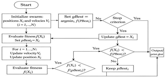
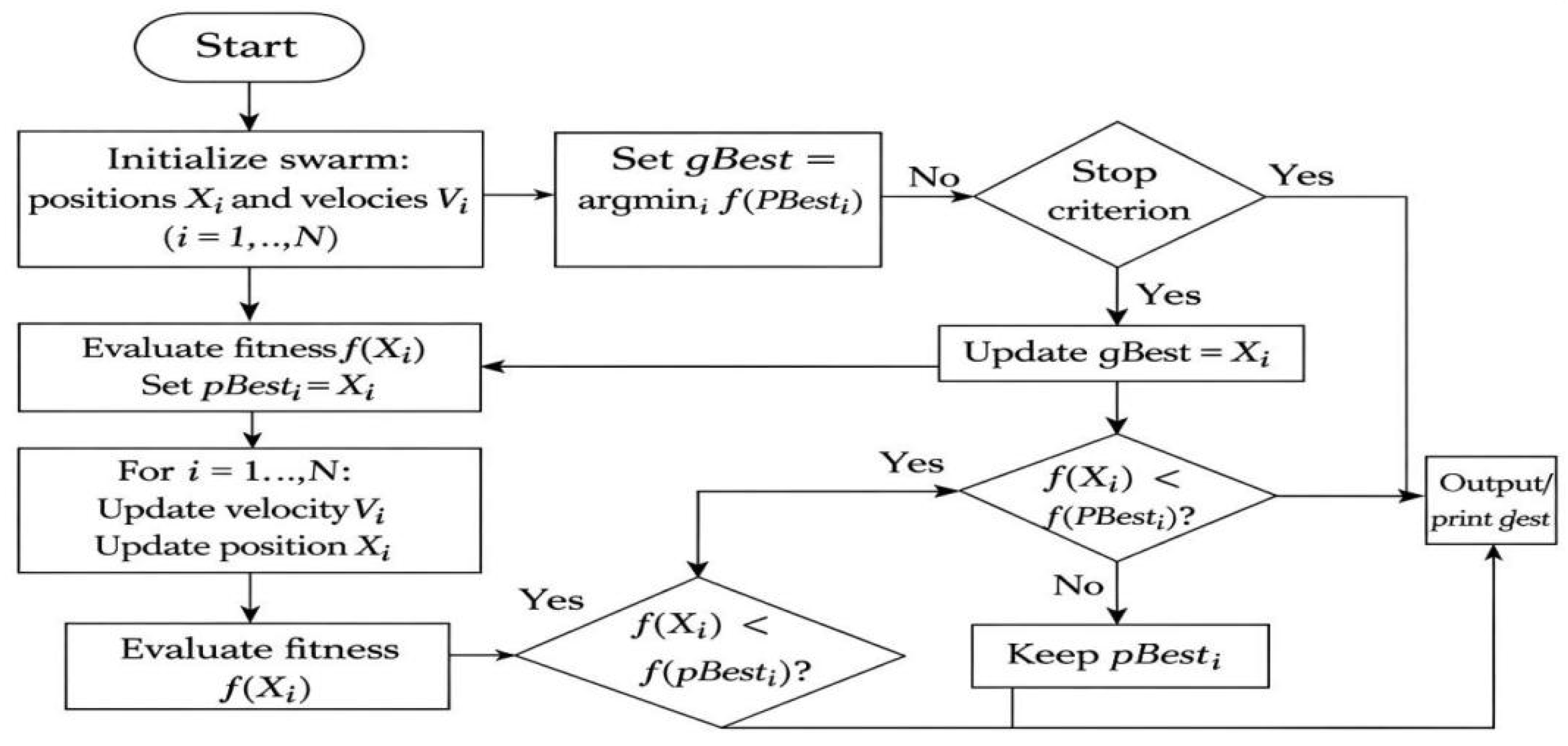
As illustrated in Figure 1, the PSO procedure starts by initializing particle positions and velocities, evaluates each particle’s fitness, and updates personal best (pBest_i) and global best (gBest) iteratively until the stopping criterion is met. In our setting, each particle encodes a candidate fusion weight α∈[0,1]\alpha \in [0,1]α∈[0,1], and the fitness is defined as the validation MAE of the hybrid forecast in Equation (7). The final gBest is then used as the fixed fusion weight for test–set evaluation.

Figure 1. Parameter settings and workflow summary for PSO–based fusion weight optimization.

2.6. Prophet–LSTM Hybrid Framework with PSO–Based Weight Tuning

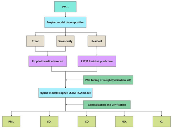
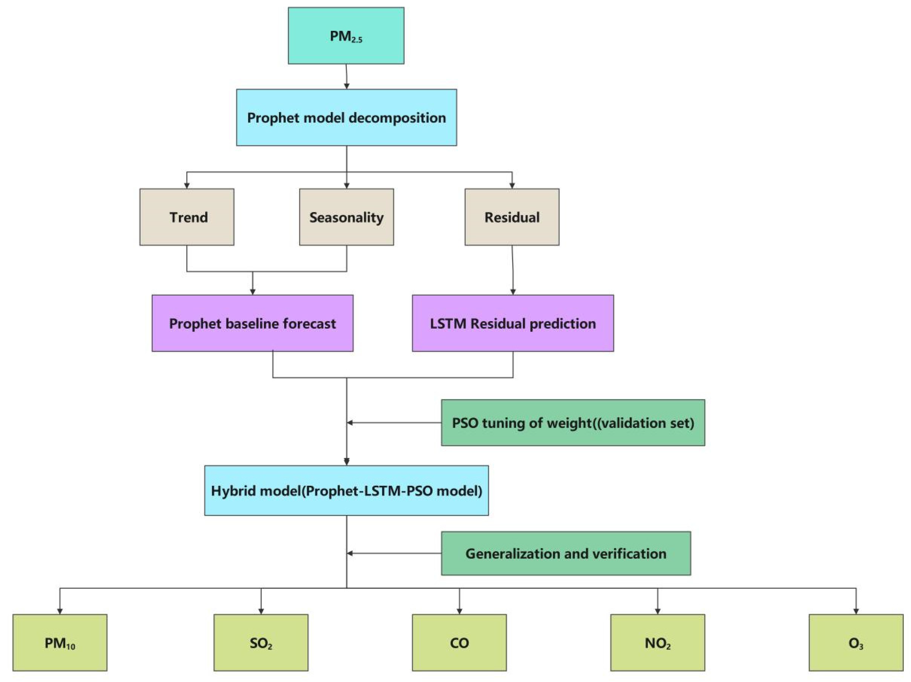
The workflow is summarized in Figure 2. We first fit Prophet on the training period to obtain the baseline one–step–ahead forecast ${\widehat{\mathbf{y}}}_{\mathbf{t}}^{\mathbf{P}}$, which captures low–frequency components (trend and seasonality). In parallel, an LSTM model is trained to produce a one–step–ahead forecast ${\widehat{\mathbf{y}}}_{\mathbf{t}}^{\mathbf{L}}$, which captures short–term nonlinear fluctuations. Finally, the hybrid forecast is computed via Equation (7), where the fusion weight α is tuned on a validation subset via PSO to avoid using test information during model selection. The tuned model is evaluated on the held–out test set via the MAE, MSE, and RMSE.

Figure 2. Framework of the hybrid Prophet–LSTM model with improved PSO.

2.7. Evaluation Metrics

The average absolute error (MAE), root mean square error (RMSE) and mean square error (MSE) are selected to estimate the prediction results of the different models. The smaller the values of the three indicators are, the smaller the prediction error of the model. Their expressions are shown in Equations (8)–(10):

$$\mathbf{M}\mathbf{A}\mathbf{E}={\displaystyle \frac{1}{\mathbf{n}}}\sum _{\mathbf{i}=1}^{\mathbf{n}}\left|\widehat{{\mathbf{y}}_{\mathbf{i}}}-{\mathbf{y}}_{\mathbf{i}}\right|$$

(8)

$$\mathbf{R}\mathbf{M}\mathbf{S}\mathbf{E}=\sqrt{{\displaystyle \frac{1}{\mathbf{n}}}\sum _{\mathbf{i}=1}^{\mathbf{n}}{\left({\mathbf{y}}_{\mathbf{i}}-\widehat{\mathbf{y}}\right)}^2}$$

(9)

$$\mathbf{M}\mathbf{S}\mathbf{E}={\displaystyle \frac{1}{\mathbf{n}}}\sum _{\mathbf{i}=1}^{\mathbf{n}}{\left({\mathbf{y}}_{\mathbf{i}}-\widehat{\mathbf{y}}\right)}^2$$

(10)

where ${\mathbf{y}}_{\mathbf{i}}$ is the true value, $\widehat{{\mathbf{y}}_{\mathbf{i}}}$ is the estimated value, $\mathbf{i}=\mathrm{1,2},\dots ,\mathbf{n}$, and $\mathbf{n}$ is the sample size.

All the MAE/MSE/RMSE values reported in this paper are computed on the original concentration scale. Specifically, for LSTM–based models, predictions are first inverse–transformed back to the original units (e.g., μg·m⁻³ for PM) before calculating the metrics, so that the reported errors retain physical meaning.

Note that the MAE and RMSE are scale dependent; therefore, absolute MAE/RMSE values are not strictly comparable across different pollutants with different numeric ranges.

Rationale for appraisal criteria. MAE and RMSE were chosen because they are widely used and easily interpretable error measures in air quality forecasting: MAE reflects the typical absolute deviation, whereas RMSE penalizes larger episodic errors more strongly, which is important for pollution episodes. The MSE is reported for completeness and consistency with prior hybrid forecasting studies. Since these metrics are scale dependent, we compute them on the original concentration scale after inverse transformation for the LSTM–based outputs to preserve their physical meaning and reproducibility.

3. Results

3.1. Comparison of Results

3.1.1. Experimental Results

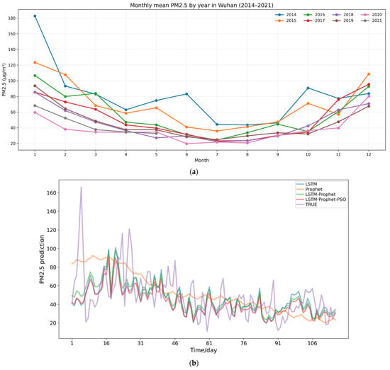
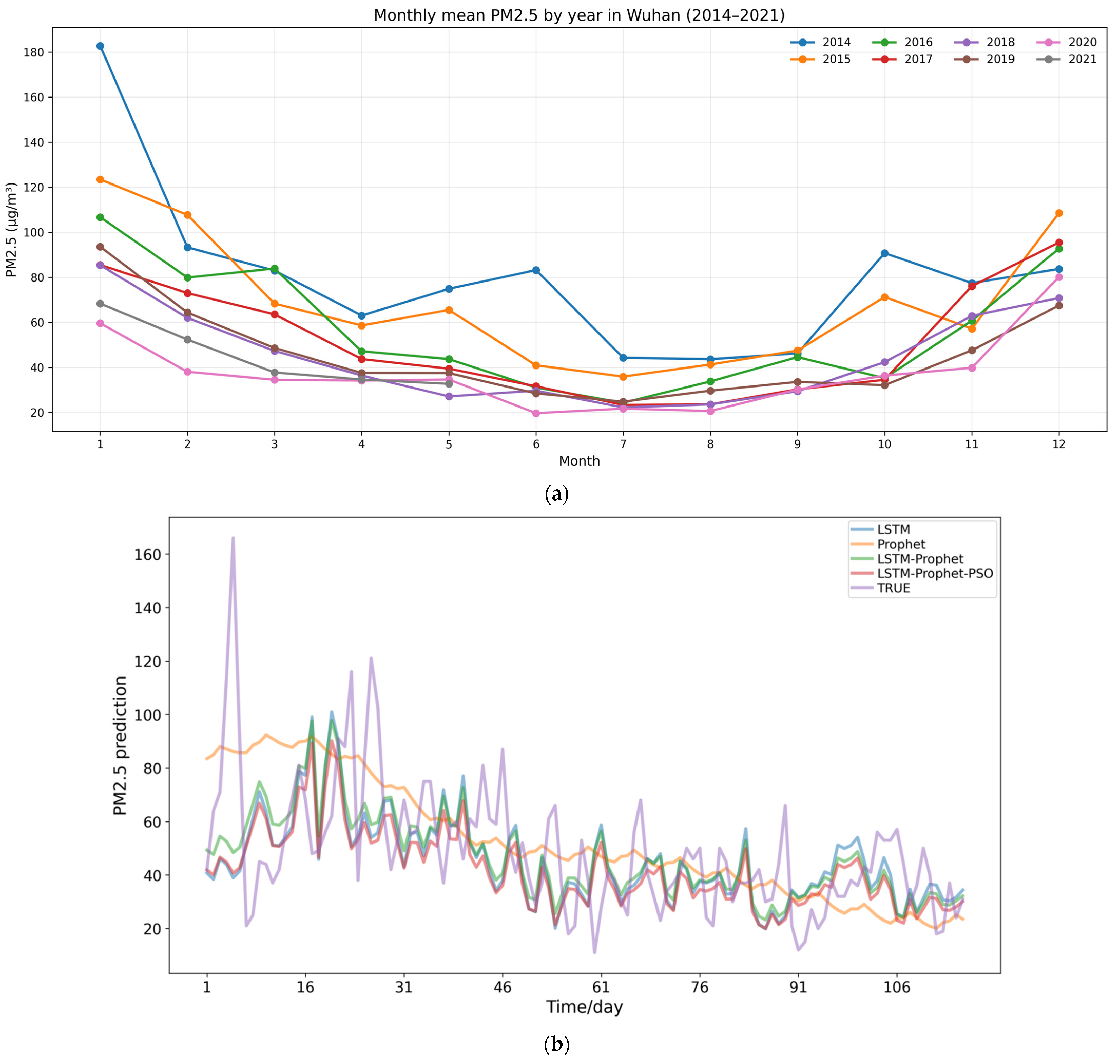
Following Prophet decomposition, the annual component reveals a pronounced seasonal cycle of PM_2.5 in Wuhan, with higher concentrations in winter (December–February) and lower concentrations in summer (June–August). Figure 3a visualizes this seasonality from a multiyear perspective by plotting the monthly mean PM_2.5 for each individual year (2014–2021), where the x–axis denotes the calendar month and the y–axis denotes the monthly averages computed from daily observations within the corresponding year. Despite interannual differences in magnitude, all years exhibit a consistent “winter–high/summer–low” pattern, indicating a stable annual cycle that is suitable for seasonal modeling. Figure 3b compares the one–step–ahead predictions of the four models (LSTM, Prophet, Prophet + LSTM, and Prophet + LSTM optimized by the improved PSO) with the observed PM_2.5 over the test period. The Prophet–only model generates a smooth trajectory that captures the low–frequency trend and seasonal pattern but tends to underreact to short–term fluctuations and peak events. The LSTM–only model is more responsive to high–frequency variations; however, it exhibits higher volatility and occasional over or undershooting when abrupt spikes occur.

Figure 3. (a) Monthly mean PM_2.5 in Wuhan for each year (2014–2021). (b) Comparison of model predictions.

3.1.2. Comparative Analysis

Three models (LSTM, Prophet and Prophet–LSTM) are selected for comparison with our models, and three indicators (MAE, MSE and RMSE) are used to measure the effect of each model. Table 2 summarizes the MAEs/MSEs/RMSEs on both the training and test sets for PM_2.5, while Figure 4a,b visualize the relative error differences across the models.

Table 2. Comparison of models for PM_2.5.

Data Set	Models	MAE	MSE	RMSE
Training set	LSTM	22.530	1076.501	32.810
	Prophet	18.870	744.138	27.278
	Prophet–LSTM	15.078	510.920	22.603
	Prophet–LSTM (with improved PSO)	14.889	506.471	22.504
Test set	LSTM	18.027	637.286	25.244
	Prophet	17.504	534.825	23.126
	Prophet–LSTM	12.040	246.880	15.712
	Prophet–LSTM (with improved PSO)	11.233	225.258	15.008

Note: Considering the randomness of the model involving LSTM in each round of training, the final index values are the results obtained by averaging repeatedly. The fusion weights for the PSO–based hybrid are tuned on the validation subset and then fixed for test–set evaluation.

Figure 4. Horizontal errors of the prediction models: (a) training set; (b) test set.

Overall, the hybrid Prophet–LSTM framework reduces the number of errors compared with those of the single models on the PM_2.5 test set (Table 2). In addition, the DM test provides statistical evidence that the PSO–enhanced hybrid significantly outperforms Prophet, whereas the improvement over LSTM is not statistically significant at the 0.05 level (Table 3).

Table 3. Diebold–Mariano (DM) test on the test set (PM_2.5).

Comparison	DM (abs)	p (abs)
Hybrid_PSO vs. Prophet	−3.223	0.001
Hybrid_PSO vs. LSTM	−1.154	0.248

To assess whether the observed improvements in Table 2 are statistically meaningful rather than due to random fluctuations, we apply the Diebold–Mariano (DM) test [19] to the test–period loss differential series. We use the absolute error as the loss and compare the proposed Prophet–LSTM model with the improved PSO against Prophet and LSTM on the same test window. The DM test indicates that the hybrid model yields a statistically significant improvement over Prophet (p = 0.001268), whereas the difference relative to LSTM is not statistically significant (p = 0.248142).

3.1.3. Generalization Capability Analysis

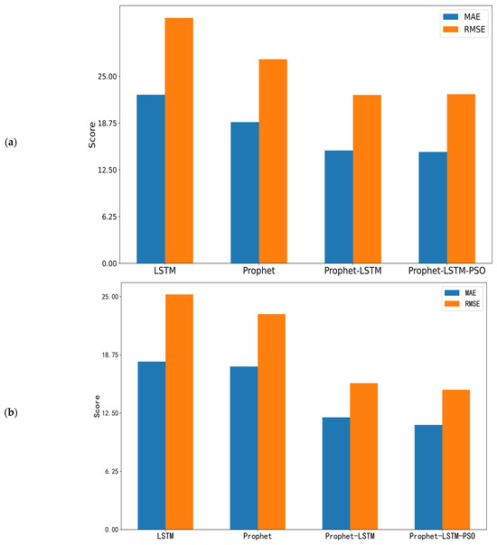
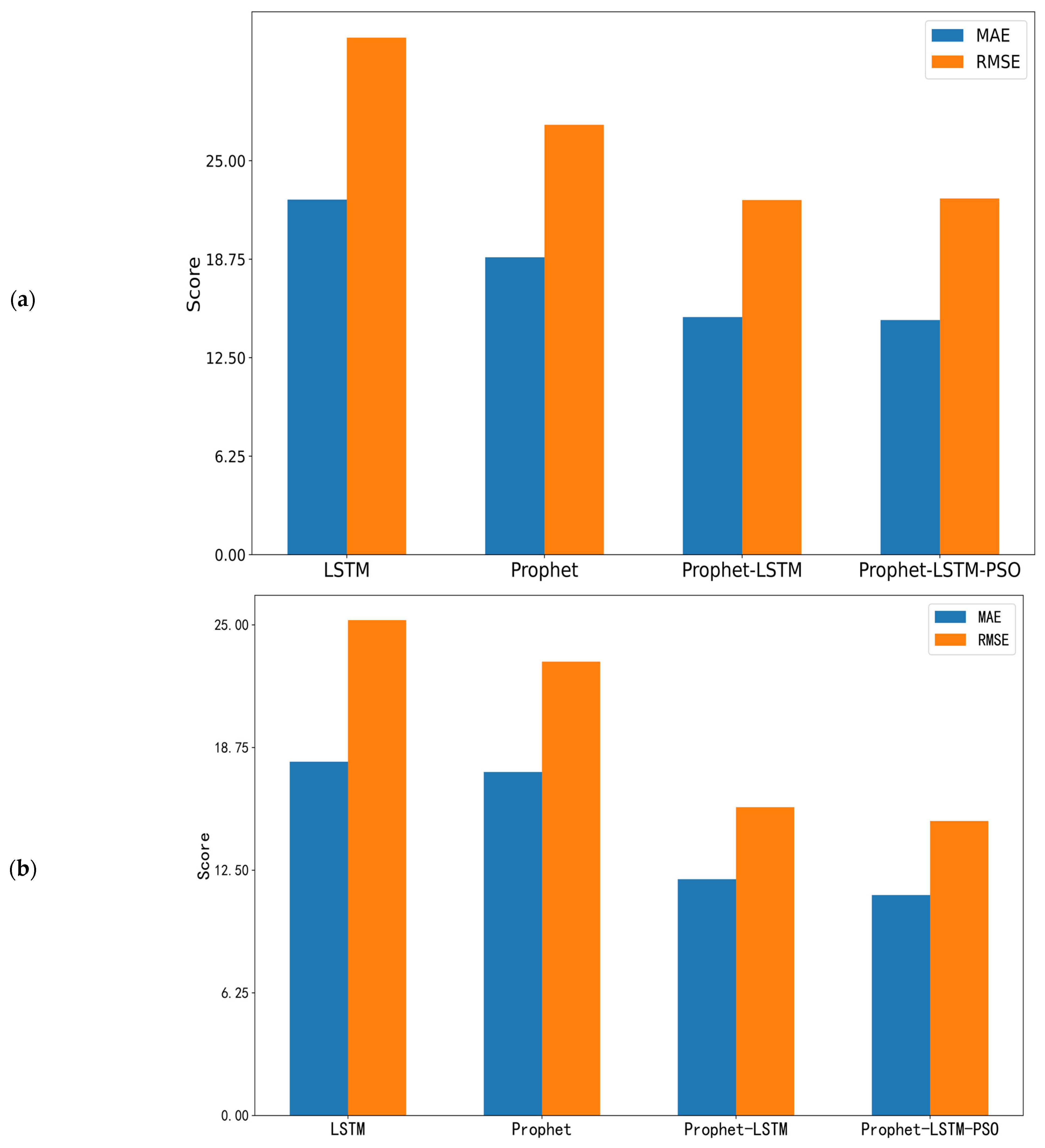
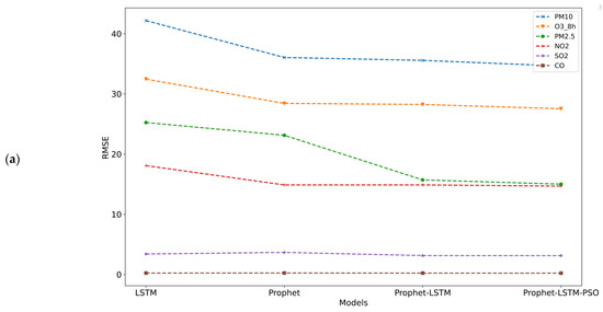
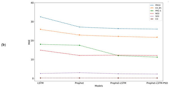
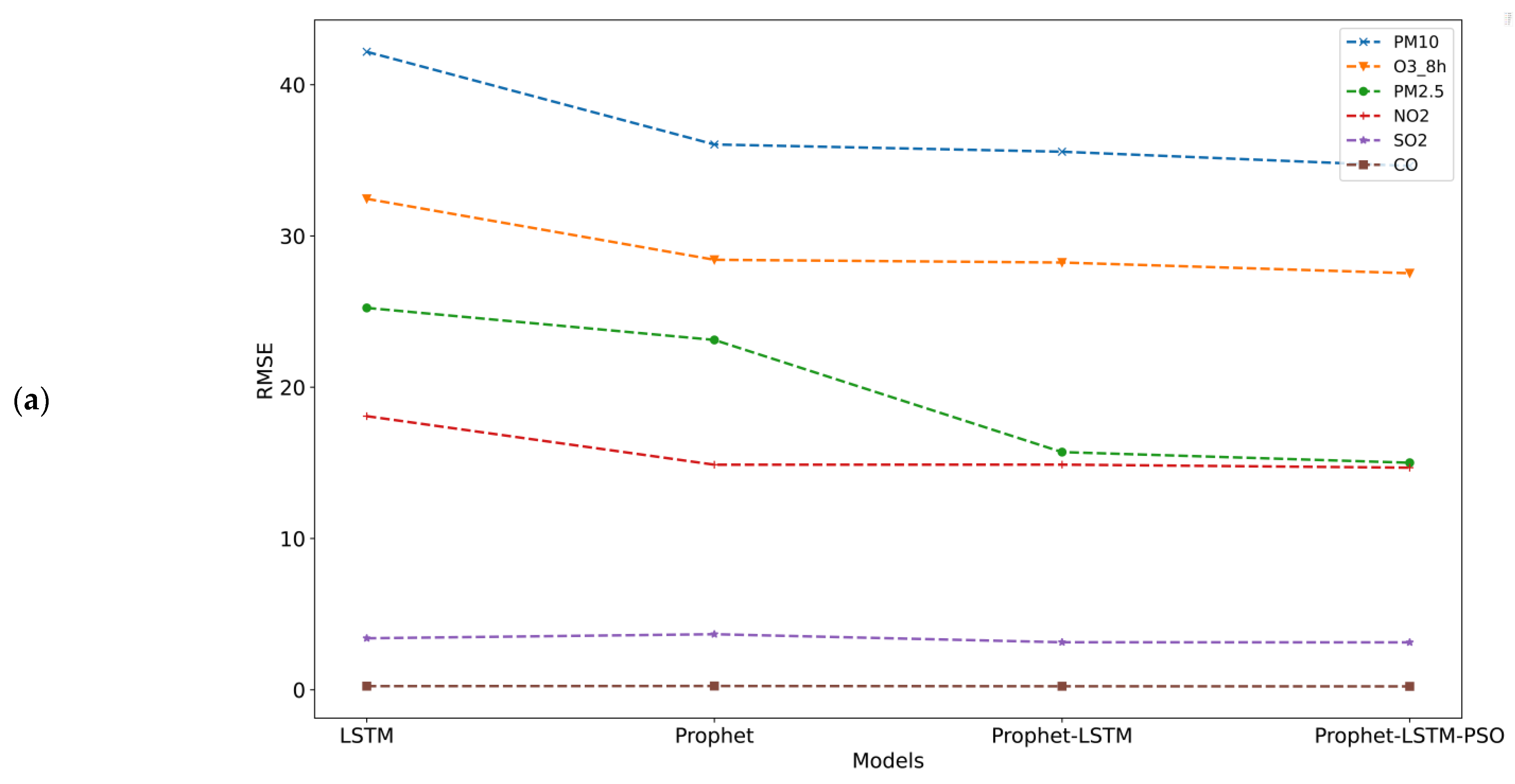
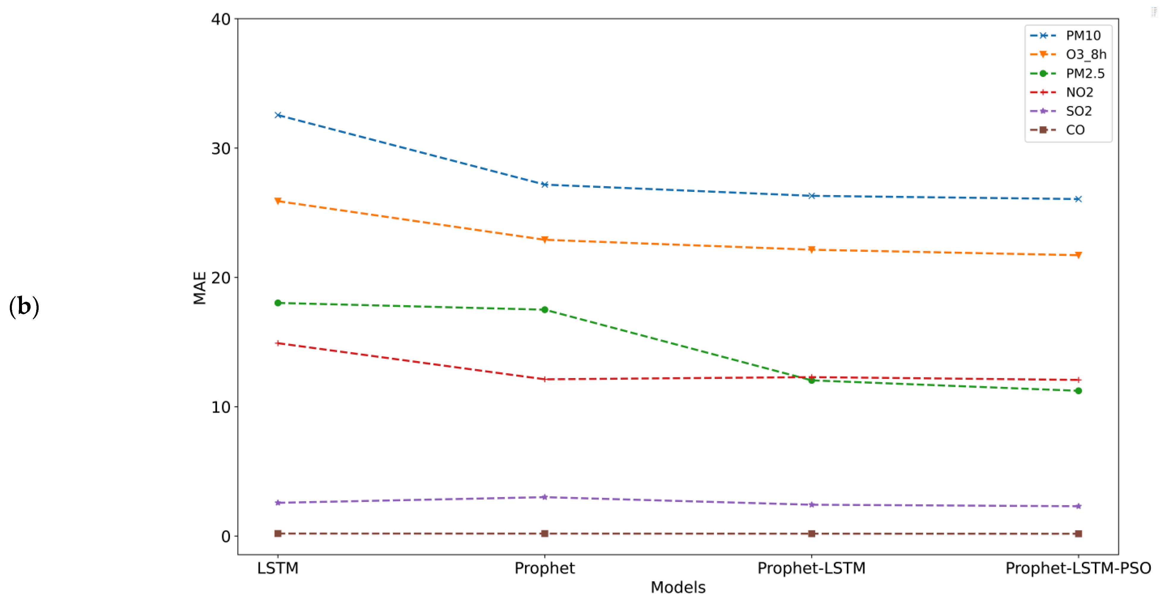
It is necessary to verify the robustness of the proposed Prophet–LSTM model with improved PSO. We therefore evaluate the model on pollutants of the same type (PM₁₀) and different types (SO₂, CO, NO₂, and O₃). The prediction results on the test set are reported in Table 4 and visualized in Figure 5.

Table 4. MAEs and RMSEs in the test set.

Index	Pollutants	LSTM	Prophet	Prophet–LSTM	Prophet–LSTM (with Improved PSO)
MAE	PM10	32.5500	27.1741	26.3076	26.0576
	SO2	2.5735	3.0088	2.4247	2.3076
	CO	0.1963	0.1928	0.1866	0.1809
	NO2	14.9144	12.1231	12.2905	12.0758
	O3	25.8970	22.9098	22.1432	21.7179
RMSE	PM10	42.1750	36.0481	35.5689	34.6279
	SO2	3.4050	3.6736	3.1421	3.1346
	CO	0.2407	0.2506	0.2329	0.2249
	NO2	18.0875	14.8783	14.8832	14.6824
	O3	32.4554	28.4266	28.2440	27.5377

Figure 5. Predicted by different pollutant concentrations: (a) MAE; (b) RMSE.

Across the evaluated pollutants, the PSO–enhanced hybrid model achieves the lowest MAE and RMSE in most cases (Table 4; Figure 5). The improvement magnitude varies by pollutant and is relatively modest for PM₁₀ and O₃, indicating that the benefit of residual modeling and weight tuning depends on the temporal variability and recurrent structure of each series. Because the MAEs/RMSEs are scale dependent and the pollutant concentration ranges differ, cross–pollutant comparisons should be interpreted cautiously. For convenience of horizontal comparison, we further aggregated the PM_2.5 test set and the indicators of other pollutants into Table 5 and provided the improvement percentage relative to the relatively optimal baseline model.

Table 5. Benchmarking.

Pollutant	Metric	LSTM	Prophet	Prophet–LSTM	Proposed (Prophet–LSTM + iPSO)	Best Baseline (%)
PM2.5	MAE	18.0275	17.5042	12.0409	11.2338	6.70
PM2.5	RMSE	25.2445	23.1263	15.7124	15.0086	4.48
PM10	MAE	32.5500	27.1741	26.3076	26.0576	0.95
PM10	RMSE	42.1750	36.0481	35.5689	34.6279	2.65
SO2	MAE	2.5735	3.0088	2.4247	2.3076	4.83
SO2	RMSE	3.4050	3.6736	3.1421	3.1346	0.24
CO	MAE	0.1963	0.1928	0.1866	0.1809	3.05
CO	RMSE	0.2407	0.2506	0.2329	0.2249	3.43
NO2	MAE	14.9144	12.1231	12.2905	12.0758	0.39
NO2	RMSE	18.0875	14.8783	14.8832	14.6824	1.32
O3	MAE	25.8970	22.9098	22.1432	21.7179	1.92
O3	RMSE	32.4554	28.4266	28.2440	27.5377	2.50

Note: Values are taken directly from the reported results tables in the manuscript (PM_2.5 from the PM_2.5 test–set table; PM₁₀, SO₂, CO, NO₂, and O₃ from the multipollutant comparison table).

4. Discussion

4.1. Interpretation of the Seasonal Cycle and Physical Drivers

This seasonal contrast is consistent with established physical drivers in Central China: the wintertime shallow planetary boundary layer (BLH) and more frequent stable stratification/temperature inversions suppress vertical mixing and dilution, whereas synoptic conditions can facilitate regional transport toward Wuhan; together, these processes lead to higher PM_2.5 levels. In addition, higher relative humidity in cold seasons can promote secondary aerosol formation through aqueous–phase chemistry, further amplifying PM_2.5 during stagnant conditions. Conversely, summertime deeper boundary layers and stronger convection enhance dispersion, while increased precipitation contributes to wet scavenging, which collectively explains the observed summer minima. Previous studies have shown that episodic biomass burning in and around Wuhan can intensify PM_2.5 pollution from summer to autumn, indicating that the seasonal cycle is shaped by both meteorology and time–varying emissions [20,21,22,23].

4.2. Interpreting Model Comparisons and Statistical Significance

By combining the two, the hybrid Prophet + LSTM model leverages Prophet to model the low–frequency structure while using LSTM to learn the residual dynamics, resulting in improved peak tracking and reduced overall error. Finally, the improved PSO further tunes the fusion weights to balance smoothness and responsiveness, yielding the closest agreement with the ground truth in Figure 3b. Hence, we interpret the hybrid advantage as robust relative to Prophet and competitive relative to LSTM under the current evaluation split. Therefore, we conclude that the proposed hybrid method is reliably better than Prophet for PM_2.5 forecasting, and it achieves numerically lower errors than LSTM on this test split, although the gain over LSTM is not statistically confirmed at the 0.05 level. The DM test suggests that the PSO–enhanced hybrid provides a statistically significant improvement over Prophet on the PM_2.5 test window (p = 0.001268), whereas the difference relative to LSTM is not significant at the 0.05 level (p = 0.248142). Accordingly, the evidence supports a robust advantage over Prophet under the current split, whereas the gain over LSTM should be interpreted as a numerical improvement without statistical confirmation in this setting.

4.3. Cross–Pollutant Generalization and Predictability

Notably, absolute MAE/RMSE values are not directly comparable across different pollutants because their units and numeric scales differ; hence, a smaller absolute error does not necessarily imply that a pollutant is intrinsically easier to forecast. To provide a more meaningful explanation of the observed performance differences, we further analyze the intrinsic predictability of each pollutant time series (see Table 6), including the relative variability (CV = std/mean), outlier rate, and weekly seasonal strength.

Table 6. Predictability diagnostics and descriptive statistics across pollutants.

Pollutant	Mean	Std	CV (Std/Mean)	Outlier Rate (IQR)	Seasonal Strength (Period = 7)	ADF p Value	N
PM2.5	54.99843	38.58663	0.701595	0.044618	0.078514	$5.42\times {10}^{-7}$	2555
PM10	85.05988	48.97303	0.575748	0.021135	0.072145	$1.39\times {10}^{-8}$	2555
SO2	14.1135	11.83224	0.838363	0.066145	0	$4.71\times {10}^{-10}$	2555
CO	1.029002	0.332877	0.323495	0.035616	0.127494	$3.26\times {10}^{-6}$	2555
NO2	45.9863	20.31439	0.441749	0.013307	0.12422	$9.58\times {10}^{-8}$	2555
O3	92.62466	48.7332	0.526136	0.000783	0.150813	$3.29\times {10}^{-4}$	2555

As summarized in Table 6, CO and NO₂ exhibit lower relative variability (smaller CV) and stronger recurrent structures, which are well captured by Prophet’s trend/seasonal decomposition and lead to a residual term that is easier for LSTM to learn. In contrast, PM_2.5 shows greater intermittency and a larger proportion of abrupt episodes, which increases residual complexity and makes accurate forecasting more challenging. These characteristics provide a practical explanation for why the hybrid framework tends to achieve better performance on some gaseous pollutants than on PM_2.5, beyond stationarity considerations alone.

4.4. Limitations and Future Work

A limitation of the current framework is that the residual term is modeled as a single component, which restricts interpretability and may leave heterogeneous error sources (e.g., abrupt episodic events versus smoother irregularities) entangled in one residual process. In addition, model performance is evaluated via a single chronological train–test split; rolling or expanding window validation is left for future work to further strengthen the robustness of the conclusions. This limitation is consistent with the fact that series with higher intermittency and a larger proportion of abrupt episodes (e.g., PM_2.5) remain more challenging to forecast than pollutants with stronger recurrent structures (Table 6). Future work will explore more structured residual decomposition and additional covariates to improve both interpretability and predictive stability.

5. Conclusions

This study proposed a hybrid Prophet–LSTM forecasting framework with PSO–based weight tuning for daily pollutant concentration prediction in Wuhan. Prophet was used to model the low–frequency components (trend and seasonality), while LSTM learned the residual dynamics, and PSO optimized the fusion weight via a validation subset to avoid test leakage. For the PM_2.5 test period, the PSO–enhanced hybrid achieves a lower MAE/RMSE than the single–model baselines and the unoptimized hybrid (Table 2). Importantly, statistical testing based on the Diebold–Mariano procedure indicates that the improvement over Prophet is significant (p = 0.001268), whereas the difference relative to LSTM is not statistically significant at the 0.05 level (p = 0.248142) (Table 3). Therefore, the proposed method can be interpreted as reliably outperforming Prophet under the current split while being competitive with LSTM with a numerically smaller error that is not statistically confirmed in this setting.

We further evaluated the framework for additional pollutants (PM₁₀, SO₂, CO, NO₂, and O₃). The hybrid model with PSO yields the lowest or near–lowest MAE/RMSE in most cases (Table 4), but the magnitude of improvement varies and can be modest for certain series (e.g., PM₁₀ and O₃). Since the MAEs/RMSEs are scale dependent and pollutants have different numeric ranges, cross–pollutant comparisons should be interpreted cautiously; the observed differences are better discussed together with time series predictability characteristics such as relative variability, outlier rates, and weekly seasonal strength (Table 6).

References

- Wang, H.; Qiu, J.; Liu, Y.; Fan, Q.; Lu, X.; Zhang, Y.; Wu, K.; Shen, A.; Xu, Y.; Jin, Y.; et al. MEIAT–CMAQ: A modular emission inventory allocation tool for Community Multiscale Air Quality Model. Atmos. Environ. 2024, 331, 120604. [Google Scholar] [CrossRef] [Scilit]
- Swathi, V.S.; Panda, S.K.; Mondal, U.; Sharma, D. Investigating dust storm dynamics and lightning interactions using Weather Research Forecasting–Chemistry (WRF–CHEM) model over India. Sci. Total Environ. 2025, 995, 180083. [Google Scholar] [CrossRef] [Scilit] [PubMed]
- Chemel, C.; Fisher, B.E.A.; Kong, X.; Francis, X.; Sokhi, R.; Good, N.; Collins, W.; Folberth, G. Application of chemical transport model CMAQ to policy decisions regarding PM2.5 in the UK. Atmos. Environ. 2014, 82, 410–417. [Google Scholar] [CrossRef] [Scilit]
- Djalalova, I.; Delle Monache, L.; Wilczak, J. PM2.5 analog forecast and Kalman filter post–processing for the Community Multiscale Air Quality (CMAQ) model. Atmos. Environ. 2015, 108, 76–87. [Google Scholar] [CrossRef] [Scilit]
- Shen, J.; Wang, X.S.; Li, J.F.; Zhang, Y. Evaluation and intercomparison of ozone simulations by Models–3/CMAQ and CAMx over the Pearl River Delta. Sci. China Chem. 2011, 54, 1789–1800. [Google Scholar] [CrossRef] [Scilit]
- Cheng, X.H.; Diao, Z.G.; Hu, J.K.; Xu, X.; Zhang, J.; Li, D. Dynamical–statistical forecasting of PM2.5 concentration based on CMAQ model and adapting partial least square regression method in China. Acta Sci. Circumst. 2016, 36, 2771–2782. [Google Scholar]
- Wu, Y.J. Source Apportionment of PM2.5 over the Beijing–Tianjin–Hebei and Surrounding Areas Based on the WRF–CMAQ/ISAM Model. Master’s Thesis, Zhejiang University, Hangzhou, China, 2019. [Google Scholar]
- Skamarock, W.C.; Klemp, J.B.; Dudhia, J.; Gill, O.; Liu, Z.; Berner, J.; Wang, W.; Powers, G.; Duda, G.; Barker, D.M.; et al. A Description of the Advanced Research WRF Model Version 4; National Center for Atmospheric Research: Boulder, CO, USA, 2019; p. 145. [Google Scholar]
- Im, U.; Markakis, K.; Unal, A.; Kindap, T.; Poupkou, A.; Incecik, S.; Yenigun, O.; Melas, D.; Theodosi, C.; Mihalopoulos, N. Study of a winter PM episode in Istanbul using the high resolution WRF/CMAQ modeling system. Atmos. Environ. 2010, 44, 3085–3094. [Google Scholar] [CrossRef] [Scilit]
- Tuccella, P.; Curci, G.; Visconti, G.; Bessagnet, B.; Menut, L.; Park, R.J. Modeling of gas and aerosol with WRF/Chem over Europe: Evaluation and sensitivity study. J. Geophys. Res. Atmos. 2012, 117, D03303. [Google Scholar] [CrossRef] [Scilit]
- Peng, J.; Han, H.; Yi, Y.; Huang, H.; Xie, L. Machine learning and deep learning modeling and simulation for predicting PM2.5 concentrations. Chemosphere 2022, 308, 136353. [Google Scholar] [CrossRef] [Scilit] [PubMed]
- Makhdoomi, A.; Sarkhosh, M.; Ziaei, S. PM2.5 concentration prediction using machine learning algorithms: An approach to virtual monitoring stations. Sci. Rep. 2025, 15, 8076. [Google Scholar] [CrossRef] [Scilit] [PubMed]
- Shen, J.; Liu, Q.; Feng, X. Hourly PM2.5 concentration prediction for dry bulk port clusters considering spatiotemporal correlation: A novel deep learning blending ensemble model. J. Environ. Manag. 2024, 370, 122703. [Google Scholar] [CrossRef] [Scilit] [PubMed]
- Qu, Y.; Qian, X.; Song, H.Q.; He, J.; Li, J.H.; Xiu, H. Machine–learning–based model and simulation analysis of PM2.5 concentration prediction in Beijing. Chin. J. Eng. 2019, 41, 401–407. [Google Scholar]
- Chen, P.S.; Zheng, Y.J.; Li, L.; Jing, T.; Du, X.X.; Tian, J.; Zhang, J.; Dong, M.; Fan, J.; Wang, C.; et al. Prediction of PM2.5 Mass Concentration Based on the Back Propagation (BP) Neural Network Optimized by t–Distribution Controlled Genetic Algorithm. J. Nanoelectron. Optoelectron. 2020, 15, 432–441. [Google Scholar] [CrossRef] [Scilit]
- Taylor, S.J.; Letham, B. Forecasting at Scale. Am. Stat. 2018, 72, 37–45. [Google Scholar] [CrossRef] [Scilit]
- Hochreiter, S.; Schmidhuber, J. Long Short–Term Memory. Neural Comput. 1997, 9, 1735–1780. [Google Scholar] [CrossRef] [Scilit] [PubMed]
- Kennedy, J.; Eberhart, R.C. Particle Swarm Optimization. In Proceedings of the 1995 IEEE International Conference on Neural Networks (ICNN’95); IEEE: New York, NY, USA, 1995; pp. 1942–1948. [Google Scholar]
- Diebold, F.X.; Mariano, R.S. Comparing Predictive Accuracy. J. Bus. Econ. Stat. 1995, 13, 253–263. [Google Scholar] [CrossRef] [Scilit]
- Jandacka, D.; Durcanska, D.; Nicolanska, M.; Holubcik, M. Impact of Seasonal Heating on PM10 and PM2.5 Concentrations in Sucany, Slovakia: A Temporal and Spatial Analysis. Fire 2024, 7, 150. [Google Scholar] [CrossRef] [Scilit]
- Shikhovtsev, M.Y.; Makarov, M.M.; Aslamov, I.A.; Tyurnev, I.N.; Molozhnikova, Y.V. Application of Modern Low–Cost Sensors for Monitoring of Particle Matter in Temperate Latitudes: An Example from the Southern Baikal Region. Sustainability 2025, 17, 3585. [Google Scholar] [CrossRef] [Scilit]
- Jandacka, D.; Durcanska, D. Seasonal Variation, Chemical Composition, and PMF–Derived Sources Identification of Traffic–Related PM1, PM2.5, and PM2.5–10 in the Air Quality Management Region of Zilina, Slovakia. Int. J. Environ. Res. Public Health 2021, 18, 10191. [Google Scholar] [CrossRef] [Scilit] [PubMed]
- Shikhovtsev, M.Y.; Molozhnikova, Y.V.; Obolkin, V.A.; Potemkin, V.L.; Lutskin, E.S.; Khodzher, T.V. Features of Temporal Variability of the Concentrations of Gaseous Trace Pollutants in the Air of the Urban and Rural Areas in the Southern Baikal Region (East Siberia, Russia). Appl. Sci. 2024, 14, 8327. [Google Scholar] [CrossRef] [Scilit]
Disclaimer/Publisher’s Note: The statements, opinions and data contained in all publications are solely those of the individual author(s) and contributor(s) and not of MDPI and/or the editor(s). MDPI and/or the editor(s) disclaim responsibility for any injury to people or property resulting from any ideas, methods, instructions or products referred to in the content. |
© 2026 by the authors. Licensee MDPI, Basel, Switzerland. This article is an open access article distributed under the terms and conditions of the Creative Commons Attribution (CC BY) license.