Use of Satellite Data Products for Studying Long-Term Changes in Ambient Air Temperature, Relative Humidity and Heat Load

Abstract

Using satellite data products across 41 years, this study explores the combined effect of summer (15 May–15 September) ambient temperatures and relative humidity on the exposure to excessive heat of people living in northern Israel. Specifically, we fused 126 Landsat satellite image data collected between 1984 and 2024 with surface meteorological observations, topographical, and land-use data. The ambient temperature (T_a) was estimated by a Random Forest (RF) regression model, with the Landsat land surface temperature (LST) as its main input. A complete spatial cover of the ambient relative humidity (RH) was obtained by a hybrid model based on Bolton’s equations. Namely, we used (i) T_a estimates of the RF model to obtain the saturation vapor pressure; (ii) a spatial interpolation of dew point temperature measurements by certified meteorological stations across the whole study area; (iii) estimates of the surface air pressure based on a digital elevation model; and (iv) thermodynamic equations for calculating the ambient vapor pressure. Initially, we calculated T_a and RH at noontime in summer at all the grid cells of each Landsat image, accounting for all the qualified Landsat images in each summer. Next, we evaluated the summer-average estimates against corresponding in situ Israel Meteorological Service (IMS) stations’ average summer measurements. Finally, we studied long-term trends over the whole study area, revealing significant summer noontime long-term trends in T_a, RH and the heat index (HI) over the study area (T_a: 0.03–0.14 °C/summer; RH: 0.05–0.18%/summer; HI: 0.08–0.82 °C/summer), as well as changes in their spatial patterns.

1. Introduction

Climate change studies require long-term measurements of meteorological variables [1] and sufficient spatial cover and diversity. However, measurements of meteorological parameters often have sparse spatial resolution. This limitation is specifically severe in the Eastern Mediterranean–Middle East region (EMME), a sensitive transition zone between four Mediterranean climate sub-categories: humid Mediterranean, dry Mediterranean, semi-arid and arid [2,3]. Trend detection in this area is challenging, since the rather modest long-term changes may be masked by significant short-term variability [4]. Due to the limited cloud cover in the summer in the East Mediterranean, satellite imagery can provide enhanced retrieval of satellite products with extended spatial cover [5]. However, data retrieved by instruments mounted on sun-synchronous low-polar-orbit satellites may suffer from limited temporal resolution due to the satellite revisit period, which depends on the swath of the satellite-mounted sensor. In this study, we made use of Landsat data products, which enabled comprehensive spatial coverage at high resolution over the study area while sacrificing the temporal resolution. Yet, presumably, the 16-day revisit period of Landsat is fit for studying long-term trends.

The World Meteorological Organization considers a thirty-year period to be the minimum period for studying climate. Thus, when studying climate change, records from more than thirty years are required to examine long-term trends [6]. There are only two satellites with extended archives that contain satellite imagery products over a period of >35 years: TIROS (NOAA) and Landsat (NASA). Among these two, only the Landsat archive contains multi-spectral spatial information at a 30 m spatial resolution suitable for estimating small-scale spatial variability [7]. Since 1984, Landsat has gathered thermal band data through its Thermal Infra-Red Sensor (TIRS), which collects spectral signatures that are used to assess the surface temperature [8,9,10,11]. Since Landsat is a sun-synchronous low-polar-orbit satellite (morning overpass time between 10:00 and 11:00 a.m. local time) with a relatively low temporal resolution (revisit period of 16 days), using Landsat data products represents a tradeoff between the high spatial resolution of the Landsat images, which enables meaningful spatially varied patterns to be studied, and their relatively poor temporal resolution, which results in the availability of only three–four images per summer, even in regions with clear sky conditions. Yet, the extended Landsat image archive may compensate for its poor temporal resolution when climate change is studied [12]. The large image database requires the development of reliable and consistent models for estimating ambient temperature and relative humidity, as satellite products have been retrieved by different sensor generations over the years in the different Landsat missions (Landsat 5 to Landsat 9).

For studying long-term exposure to excessive heat, the ambient temperature (T_a) and relative humidity (RH) were combined into a single parameter—the heat index (HI)—using Fischer and Schar’s (2010) equation [13,14]. In general, retrieved satellite products are not identical to surface-measured variables, with the latter being the variables commonly used for long-term change detection. For example, for tracking long-term changes in HI, one needs to account for changes in the air temperature at 2 m a.g.l. (T_a) rather than for changes in the surface temperature (ST), which is the common climate change marker above land (LST) or ocean (SST). In summer in the study area, the difference between Earth’s radiative “skin” temperature, i.e., Landsat’s land surface temperature (LST) product, and T_a observations at the Israel Meteorological Service (IMS) meteorological stations can reach >5 °C (mean difference = 3.3 °C, mean RMSE = 4.2 °C; Figure S1). Nonetheless, it is common to estimate the air temperature based on satellite-retrieved LST, which represents a blend of thermal signatures from tree canopies, bare soil, asphalt roads, building rooftops, etc. [15]. As for relative humidity, some satellite instruments, e.g., MODIS, can measure the integrated atmospheric column water content [16]. Yet, due to the varying and complex humidity profile in the atmosphere, traditional methods for deriving RH from remotely sensed data usually require in situ meteorological observations [17]. Moreover, RH is spatially patchier than T_a, since it is affected by numerous land-use/land-cover features, as well as by the wind field (speed and direction) and the presence of airborne particles (dust, sulphates, nitrates, black carbon [16]).

Despite the large body of scientific literature that has utilized different indicators to examine climate change, most studies have accounted only for the air temperature or the land surface temperature (LST), overlooking the different spatiotemporal variability in ambient air temperature and heat load [18,19]. To address this gap, this work aims to: (a) develop a unified modeling method for completing and fusing archived satellite data and ground-based meteorological measurements, (b) improve the estimation of historic exposure to severe heat, and (c) assess long-term changes in spatiotemporal patterns of climate variables over a complex terrain.

In this work, we estimated the air temperature and relative humidity at 14:00 in each grid cell on dates in which Landsat imaginary data were available in the summers (15 May–15 September) of 1984–2024. For this, we developed two models: (a) a Random Forest (RF) model for T_a estimation, with the main input being the retrieved Landsat LST, and (b) a hybrid model for estimating the RH based on T_a from the RF model and a thermophysical model for the ambient water vapor, using in situ surface measurements of the dew-point temperature at certified IMS stations as input. Using all the qualified Landsat images in each summer (and no fewer than three images per summer), the models’ outputs enabled the estimation of the mean values at 14:00 of each meteorological variable at each grid cell for each summer between 1984 and 2024. The models’ results are three raster layers per summer (spatial resolution: 30 m) of estimated air temperature (T_a), relative humidity (RH), and the heat load (HI). This enabled us to study spatiotemporal changes in the patterns of these meteorological parameters in northern Israel over a period of 41 years.

2. Methods

2.1. Study Area

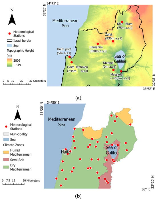
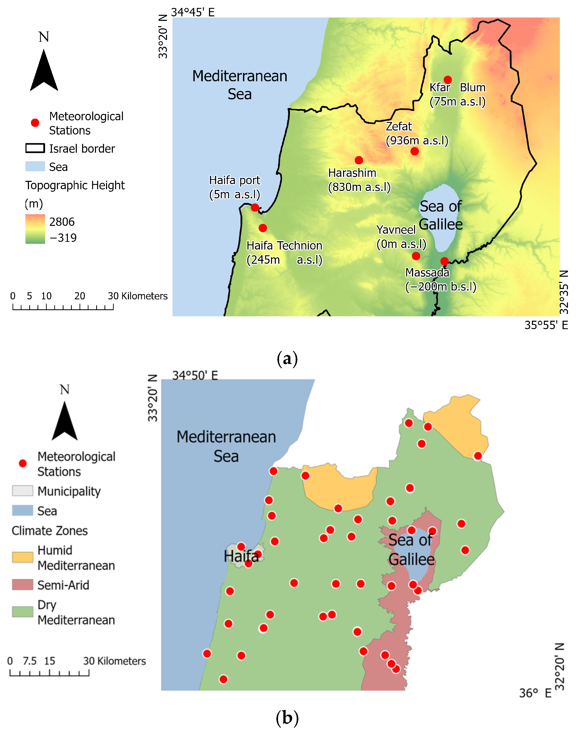
The study area covers the whole of northern Israel, from Hadera to the Lebanon border, and is contained within one Landsat imaging sheet. Due to the Syrian–African Rift, and specifically the Dead Sea Transform, the area is characterized by sharp topographical gradients, with the lowest point in the study area being the Sea of Galilee (−210 m b.s.l) and the highest point being Mount Hermon (2814 m a.s.l), just about 70 km apart from each other (Figure 1a). In the west, the area is characterized by a narrow (north–south) coastline of the Eastern Mediterranean Basin, which is a significant source of humidity in the summer months [14]. The study area experiences three Mediterranean climate sub-categories: humid Mediterranean, dry Mediterranean, and semi-arid. Figure 1b depicts the spatial pattern of these three Mediterranean climate sub-categories in the study area, as well as the meteorological stations whose data were used. The summers in the study area are characterized by high temperatures and high humidity along the coast, and by high temperatures and lower humidity inland [2]. The unique geoclimatic conditions in northern Israel result in areas that are characterized by severe heat loads.

Figure 1. (a) The topographical gradients in the study area. (b) The overall footprint of the Landsat image sheet, with the colored polygons showing the spatial pattern of the Mediterranean climate sub-categories in the study area. The red dots indicate the locations of the meteorological stations used in this study.

2.2. Meteorological Data

Meteorological data (air temperature, T_a; relative humidity, RH; dew-point temperature, T_d), measured at certified Israel Meteorological Service (IMS) stations scattered in the study area from the summers of 1984–2024 (the study period), were obtained from the IMS archive [20]. It is noteworthy that until the early 2000s, 59 IMS meteorological stations were situated in rural areas, while only 11 IMS stations were situated in urban areas. This pattern changed due to rapid urbanization and population growth, and currently, many of the IMS stations are situated in urban-affected environments [21]. Moreover, in the early period (1984–1990), the IMS measurements were gathered manually, and, in the early years, only at ~2 p.m. [22]. In the mid-1990s, the IMS stations started to report their measurements automatically, but by the beginning of the 2000s, automated IMS data collection and archiving had been implemented in more than 80% of the IMS stations. Figure S2 shows the number of IMS stations that reported in each year of the study period, and whether the data were collected manually or automatically. For consistency across the whole study period, we used only measurements taken at ~2 p.m.

2.3. Landsat Data Products

Heat load estimates were calculated at each grid cell using model estimates of the air temperature (T_a) and the relative humidity (RH), which together define human thermal comfort when exposure to direct solar radiation is ignored/irrelevant [14]. The ambient air temperature, T_a, was estimated using a Random Forest regression model whose inputs were various Landsat data products (LST, the surface albedo and emissivity, NDVI), retrieved from the Multispectral Scanner (MSS) and the Thermal Infrared Sensor (TIRS) carried on Landsat 4, 5, 7, 8, 9 (Collection 2, Level 1, spatial resolution: 30 m) (Table S1 lists the different Landsat mission instruments spectral bands). To increase the number of images that could be analyzed, we used Level 1 (Tier 1, T1) data products, which are considered suitable for time-series analysis [23,24]. However, the use of L1 data products required additional processing relative to that applied to the Level 2 (L2) data products. Specifically, while the Landsat instruments are calibrated prior to launch, constant calibration is required to offset the degradation that occurs due to the mechanical or electrical outcomes of, e.g., exposure to UV radiation [23,25]. To ensure accurate and consistent analysis, we calibrated the L1 data products using the radiometric and geometric coefficients provided for each band for converting the raw Digital Numbers (DNs) to physically meaningful Top-of-the-Atmosphere (TOA) radiance, and to the ground reflectance and brightness temperature [24].

The Landsat 4 and 5 Thematic Mapper (TM) consisted of one TIRS band (band 6, 10.40–12.50 µm) out of its seven spectral bands. The Landsat 7 Enhanced Thematic Mapper Plus (ETM+) consisted of two TIRS bands (Table S1). We used the VCID 2 high-gain band (band 62, 10.40–12.50 µm), which is more suitable for areas with moderate vegetation cover (cool surfaces) [26]. The Landsat 8 and 9 Operational Land Imager (OLI) consists of two TIRS bands in addition to nine other spectral bands (bands 10 and 11, Table S1; [27]).

In total, we used 126 qualified Landsat images, retrieved during the summers (15 May–15 September) of 1984–2024 and obtained from the USGS Global Visualization Viewer (GloVis) archive [28]. All the images were captured under clear sky conditions, i.e., with <10% cloud cover, and were used for model development and evaluation. In the pre-processing step, all the L1 images passed radiometric and atmospheric corrections, with the correction coefficients provided in the files accompanying the retrieved images. Next, the LST was retrieved from the thermal-IR (TIR) Landsat bands as follows,

$$LST={\displaystyle \frac{BT}{\left(1+0.0015\cdot BT/1.4388\right)\cdot \ln \mathsf{\epsilon }}}$$

(1)

where BT is the brightness temperature, derived from the Landsat thermal band, and ε is the surface emissivity, which accounts for the surface roughness and vegetation cover (NDVI) [29],

$$NDVI={\displaystyle \frac{NIR-R}{NIR+R}}$$

(2)

where NDVI represents a relationship between the spectral red band (R) and the near-infrared (NIR) band. For Landsat 4, 5 and 7 these bands were band 3 (0.63–0.69 µm) and band 4 (0.77–0.90 µm), respectively; for Landsat 8 and 9, these bands were band 4 (0.64–0.67 µm) and band 5 (0.85–0.88 µm), respectively.

2.4. Estimation of the Ambient Air Temperature

The Heat Index (HI) was calculated based on T_a and RH, with T_a being the air temperature at 2 m a.g.l. We developed a Random Forest (RF) regression model for estimating T_a in each grid cell based on the Landsat-retrieved LST and additional auxiliary variables, all characterized by a complete spatial cover. Specifically, the dependent variable was the measured T_a at the IMS meteorological stations (i.e., spatially discrete in situ monitoring data), and the independent variables were satellite data products (LST, NDVI, albedo, emissivity), retrieved in each grid cell of all the images, which thus have a complete spatial coverage. Moreover, since T_a generally declines with height [30], the RF model also accounted for the surface topography, with the surface elevation (per grid cell) obtained from a digital elevation model (DEM; m). The surface albedo (a) was calculated as follows [31],

$$a=0.356 {\beta }_1+0.13 {\beta }_2+0.373 {\beta }_3+0.085 {\beta }_4+0.072 {\beta }_5-0.0018$$

(3)

where β₁, β₂, β₃, β₄, and β₅ were the readings of bands 1, 3, 4, 5 and 7 in images acquired by Landsat 4, 5 and 7, or of bands 2, 4, 5, 6, and 7 of images acquired by Landsat 8 and 9 (see Table S2 for a list of processed Landsat images).

We used an RF model with Breiman’s algorithm adaptation implemented [32]. An RF model is a collection of many individual decision trees, with each tree generated based on a different subset of the training data. In general, RF models are supervised learning algorithms that require a labeled training dataset. Specifically, the development of the RF model followed two steps: a training step (based on 100 runs, with 100 trees per run) and a performance evaluation step, which used data that were set aside before the training, with a 90:10 training:evaluation ratio. Next, we used the RF model’s Feature Importance to examine the contribution of each feature to the overall estimation. Finally, the RF model was applied for estimating T_a in all the grid cells of all the images, providing a layer with complete cover of estimated T_a values in each date for which there was a qualified Landsat image (i.e., even in cells where in situ IMS measurements were not available).

Since we had only a limited number of qualified images each summer, to enable multi-year analyses but avoid bias that could result from the different number of qualified images per summer (i.e., heterogeneous sampling) along the study period, we averaged all the model estimates in each grid cell in each summer, also keeping the other cells’ statistics. To assess the performance of the summer-averaged model results in each grid cell, we compared the summer-average RF-modeled T_a at the Landsat overpass time (between 10:00 and 11:00 a.m. local time) in grid cells in which IMS stations were situated against the IMS meteorological stations’ average measurements at ~14:00. It is noteworthy that we accounted for IMS data from every day each summer, including those for which there were no Landsat images. This comparison enabled the evaluation of the summer-average model estimates in grid cells for which there were IMS meteorological records. As will be shown, we found that the summer-average T_a estimates by the RF model represented the summer-average in situ T_a measurements reasonably well.

2.5. Relative Humidity

The relative humidity (RH, %) is the ratio between the actual vapor pressure (e, mb) and the saturation vapor pressure at the same temperature (e_s, mb):

$$RH = \left(e/e_s\right)·100$$

(4)

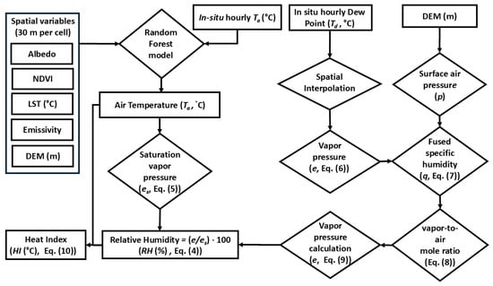
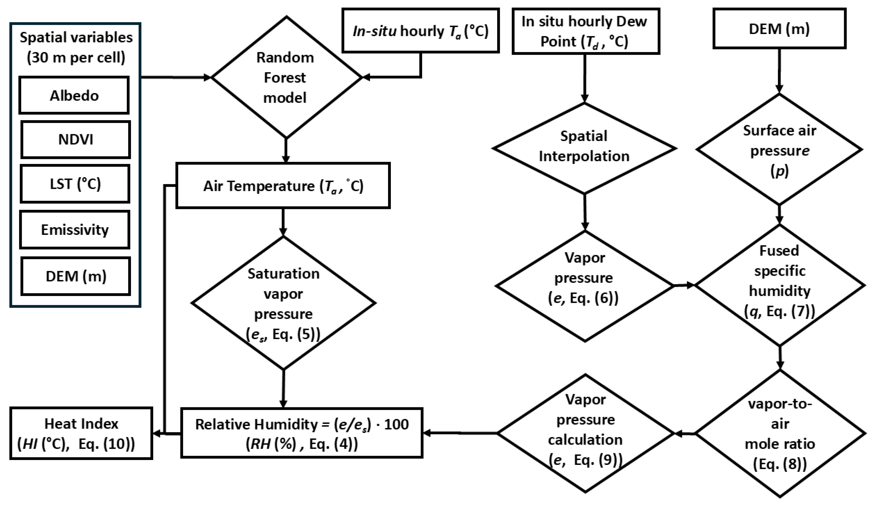
Figure 2 illustrates in detail how the relative humidity was estimated. Briefly, after the air temperature has been estimated, the relative humidity can be estimated using Bolton’s [33] scheme. Specifically, the saturation vapor pressure (e_s) was obtained based on the modeled air temperature, T_a (°C),

$$e_s=6.112\cdot \exp \left\{{\displaystyle \frac{17.67\cdot T_a}{T_a+243.5}}\right\}$$

(5)

Figure 2. Flowchart depicting the estimation of ambient temperature, T_a, relative humidity, RH, and the heat index (HI).

The actual vapor pressure (e) was estimated as follows: (i) a first estimate was obtained by using Equation (5), but instead of using the air temperature, T_a, the dew point temperature, T_d (°C), was used,

$$e=6.112\cdot \exp \left\{{\displaystyle \frac{17.67\cdot T_d}{T_d+243.5}}\right\}$$

(6)

To be able to perform this in each grid cell of the Landsat image, dew point temperature measurements from all the certified IMS meteorological stations that reported on each day were spatially interpolated using Inverse Distance Weighing (IDW) with a power of 2 (representing steep decay, as physically expected for T_d). The accuracy of this first estimate of e depends on the number of T_d data points (i.e., the number of certified IMS meteorological stations that reported dew point temperature on each day), their spatial distribution, and on the rather smooth T_d interpolation map, which often may not correctly represent the actual patchy nature of the T_d pattern at the surface. (ii) Hence, to improve the estimation of the vapor pressure, we combined the estimated e (Equation (6)) with time- and date-specific thermodynamic information using the schemes of Bolton [33] and Cook [34]. Namely, from the basic thermodynamics principles of moist air, the specific humidity (q, kg_{water_vapor}/kg_{moist_air}) at the IMS meteorological stations, which is hard to distinguish from the mixing ratio (r, kg_{water_vapor}/kg_{dry_air}), was estimated as

$$q={\displaystyle \frac{0.622\cdot e}{p-0.378\cdot e}}$$

(7)

with the atmospheric pressure at the surface (p, mb) estimated by an empirical formula [35] based on elevation data obtained from a digital elevation model (DEM, 30 m resolution). The water vapor-to-air mole ratio, x_w, was then calculated as

$$x_w={\displaystyle \frac{q\cdot M_a}{M_w-q\cdot \left(M_w+M_a\right)}}$$

(8)

where M_a and M_w are the molecular masses of dry air and of water, respectively. By definition, the vapor pressure is [34]

$$e=p·x_w$$

(9)

2.6. Heat Index

The heat index (HI, °C) was calculated using the Fischer and Schar [13] equation,

$$\begin{array}{l}HI=-8.79+1.61\cdot T_a+2.34\cdot RH-0.15\cdot T_a\cdot RH-0.012\cdot T_a^2-0.016\cdot R{H}^2\\ \hspace{1em}\hspace{1em}+0.0022\cdot T_a^2\cdot RH+0.00073\cdot T_a\cdot R{H}^2-0.0000036\cdot T_a^2\cdot R{H}^2\end{array}$$

(10)

However, when the calculated HI was <27 °C, it was recalculated using Anderson et al.’s equation [7],

$$HI=0.61\cdot T_a+0.047\cdot RH-23.5$$

(11)

The estimated HI, whose calculation combined the RF model’s estimated ambient temperature (T_a) and the hybrid model’s estimated relative humidity (RH), was evaluated against HI values calculated based on in situ observations of T_a and RH at the IMS meteorological stations.

2.7. Model Evaluation

The models were evaluated as follows. First, on dates when Landsat images were available, the estimated meteorological parameters (T_a, RH) on the satellite overpass time (~10:30 a.m.) were evaluated against corresponding measurements from 14:00 at all the certified IMS meteorological stations in the study area (it is noteworthy that the training of the RF model accounted for the time difference between the two measurements). To enable the study of long-term trends while addressing the non-uniform availability of qualified Landsat images across the summers over the study period, 1984–2024, we averaged the model results in all the grid cells, including only those obtained on dates in which qualified Landsat images were available, and the IMS stations’ in situ observations (which were available for all days in all the summers in the study period). We evaluated the former against the latter in grid cells in which the IMS stations were situated using two metrics: the root mean squared error (RMSE) and the Pearson regression coefficient.

2.8. Long-Term Trends

Long-term trends of the summer-average modeled T_a, RH, and HI over the four decades were examined using the non-parametric Mann–Kendall (MK) test, with a significant monotonous trend (p < 0.05) reported when $\left|{\left(z-\mathrm{score}\right)}_{MK}\right|\ge 1.96$, with its sign implying a downward (−) or upward (+) trend, i.e., a decrease/increase in the long-term climatic conditions, respectively. Specifically, we used the MK test to quantify the intensity of the change (i.e., the Sen’s slope over the study period) and its sign (positive/negative, based on the reported Mann–Kendall S score). In addition, we calculated the Kendall rank coefficient (Kendall’s τ) and examined whether ordinal associations existed between the examined variables. Trend analyses were performed both per grid cell as well as in buffer zones of 0.5 km around six meteorological stations that operated throughout the study period and that differ from each other in their topographical height (range: from Kibbutz Massada at 200 m b.s.l. to Tzfat at 936 m a.s.l.) and climate (e.g., Harashim and Tzfat—Humid Mediterranean climate, Haifa and Kfar Blum—Dry Mediterranean climate, Massada and Yavneel—Semi-Arid climate). Both analyses served to study spatial patterns (using ArcGIS Pro v3.6). Next, using the Mann–Kendall analysis, we performed trend detection over 41 summers to examine long-term temporal trends in terms of intensity and direction.

3. Results

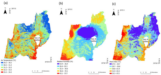
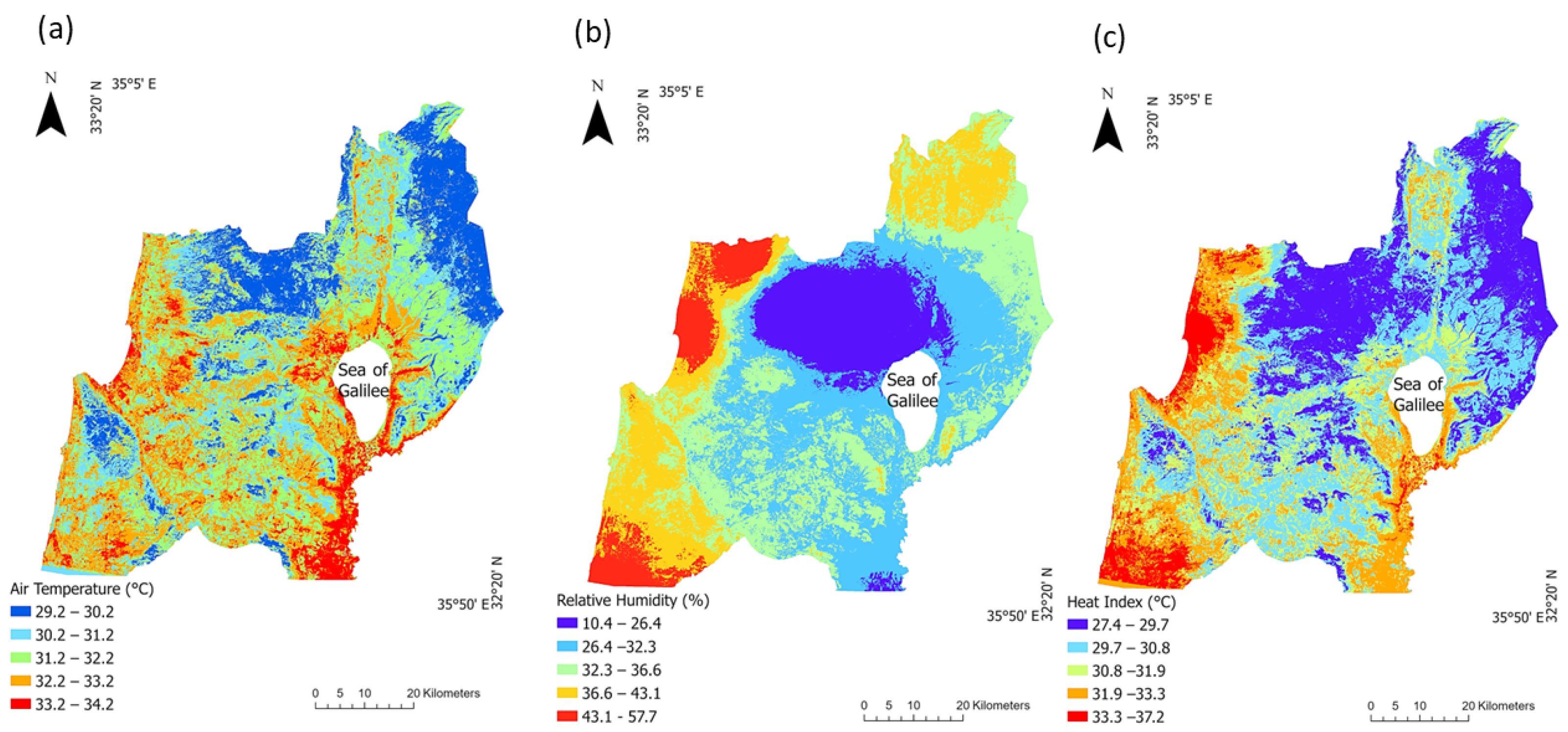
Overall, we used 126 qualified Landsat images for estimating the ambient temperature (°C), relative humidity (%) and heat load (°C) in the summers (15 May–15 September) of 1984–2024, with ≥3 images per season (Table S2 lists the dates on which the images were retrieved). Figure 3 depicts an example of complete-cover model outcomes, which were obtained for 28 August 1989: (a) the Random Forest-model-estimated ambient temperature, (b) the hybrid-model-estimated relative humidity, and (c) the estimated heat index.

Figure 3. Estimated meteorological conditions on 28 August 1989: (a) ambient temperature (estimated by the Random Forest model); (b) relative humidity (estimated by the hybrid model); and (c) heat load (i.e., the heat index, calculated by Equations (10) and (11)).

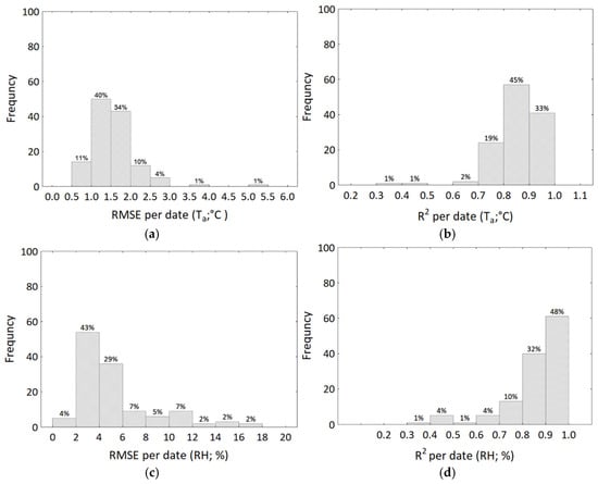
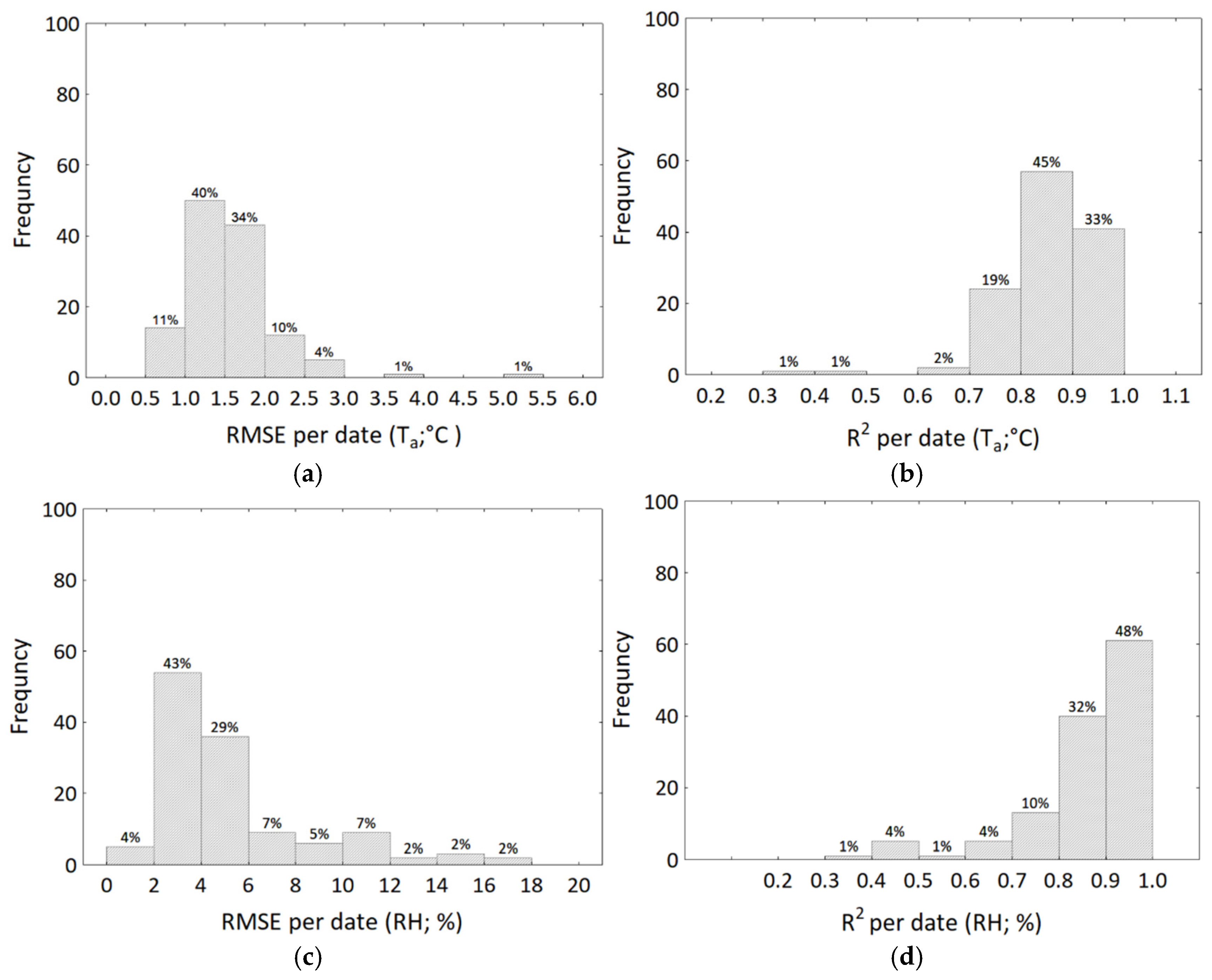
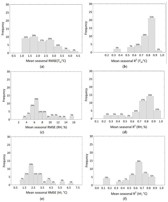
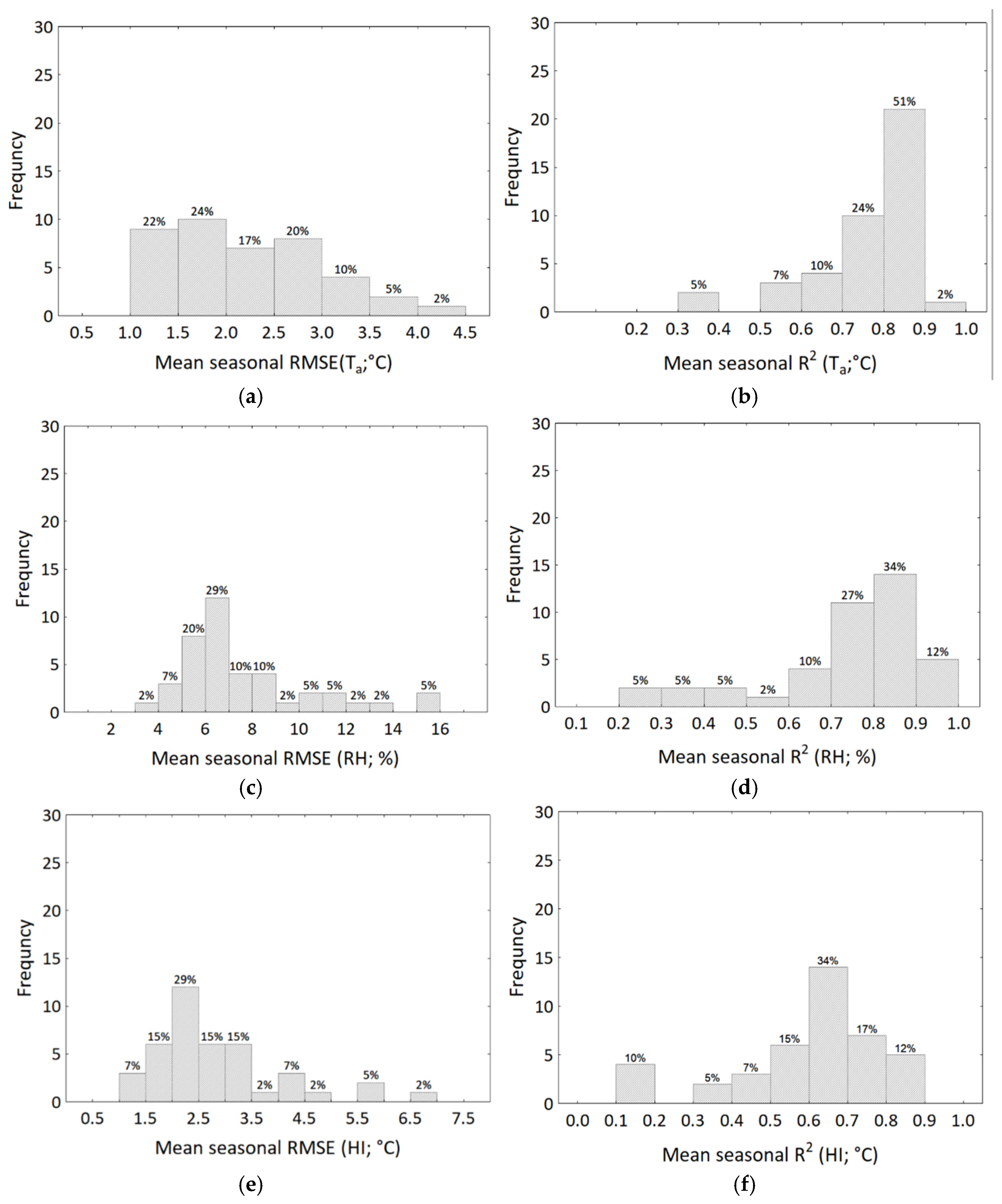
We evaluated our estimations against in situ measurements by the IMS meteorological stations using (a) records gathered by the IMS meteorological stations at ~14:00 on days for which qualified Landsat imagery data exist, and (b) their summer averages. The overall accuracy of the T_a model estimates over the whole study period was: RMSE—1.58 °C, R²—0.86, RMSE < 2 °C for 85% of the T_a estimates (Figure 4a). Only about 6% of the T_a estimates had RMSE > 2.5 °C (Figure 4a), and R² > 0.7 for 97% of the T_a estimates (Figure 4b). It is noteworthy that this performance was achieved despite the limited number of qualified Landsat images available.

Figure 4. Performance of the RF model (T_a; (a,b)) and hybrid model (RH; (c,d)) based on 126 qualified Landsat images over the study area between 1984 and 2024. (a,c) RMSE, (b,d) R².

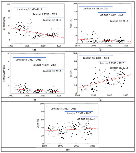
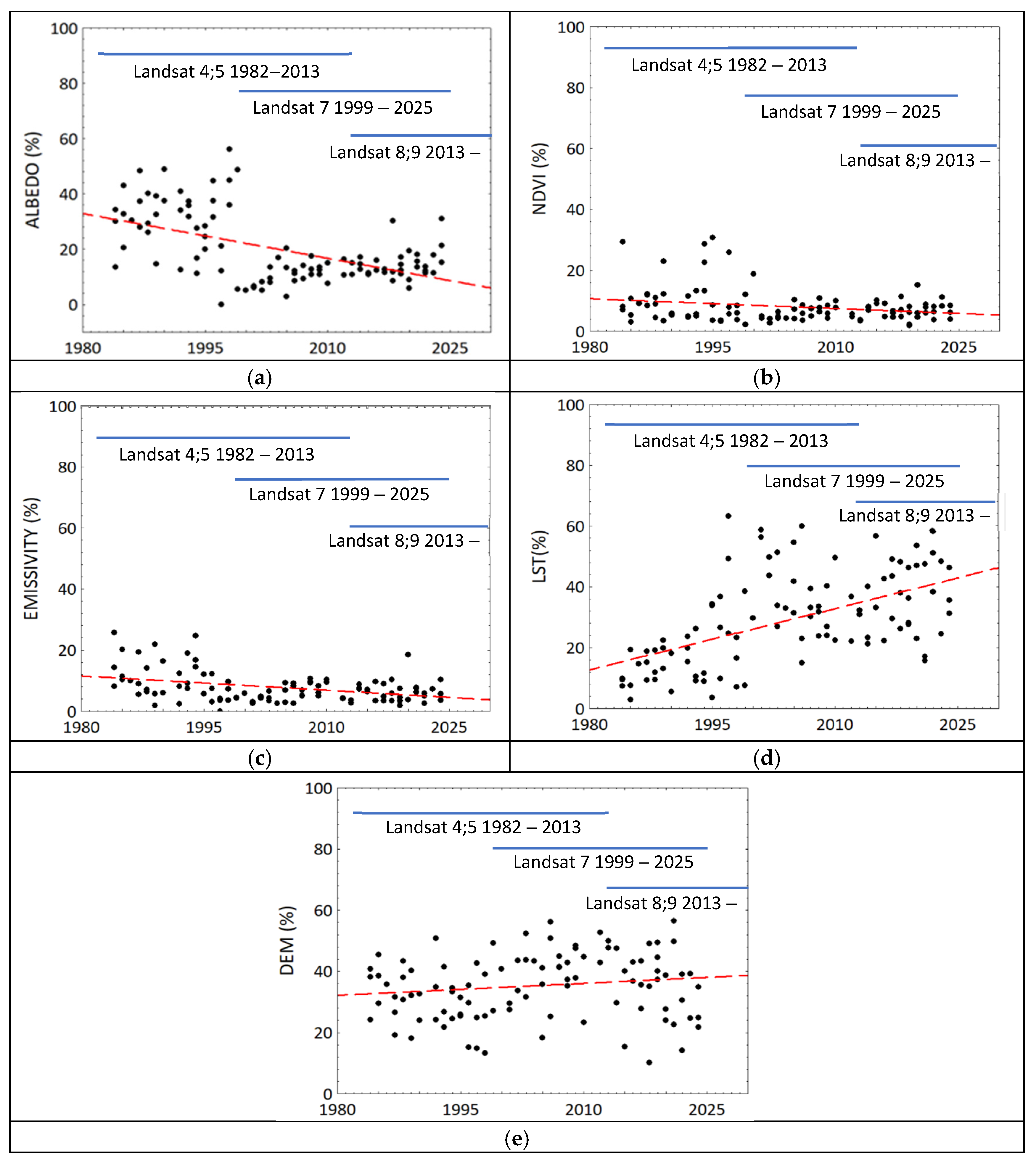
The RF model also reported the Feature Importance (%) for the input features (the explanatory variables: elevation, NDVI, surface emissivity, albedo, LST). The change in the contribution of each feature to the T_a estimates over the study period (41 years) was examined using the Spearman correlation coefficient (significance, p < 0.05). While the elevation (DEM, r = 0.28) and the LST (r = 0.56) showed significant positive (increasing) trends (Figure 5), the albedo (r = −0.52) and the emissivity (r = −0.34) showed significant decreasing trends. The NDVI showed a non-significant decreasing trend (r = −0.16, p = 0.11). It is noteworthy that such trends could have also been related to changes in the sensors across the different Landsat missions [23,25]; however, Figure 5 suggests that these changes do not align with the discerned jumps in the contributions of the different variables due to Landsat sensor changes (e.g., Figure 5a), thus the observed trends seem to not have resulted from measurement error/bias. Similarly, the overall accuracy of the RH hybrid model estimates was: RMSE—5.26%, R²—0.86, RMSE < 10% for 88% of the RH estimates (Figure 4c), and R² > 0.8 for 80% of the RH estimates (Figure 4d).

Figure 5. The Random Forest model (RF) Feature Importance (FI) results in each summer throughout the study period. The FI reports the contribution of each feature to T_a estimation. (a) albedo (a), (b) vegetation cover (NDVI), (c) emissivity (ε), (d) land surface temperature (LST), and (e) elevation (DEM). Each dot in each figure was obtained from an RF model that was developed for a qualified image. The red dashed lines are the linear regressions reported in the text.

For studying long-term trends, summer-average T_a, RH, and HI values were calculated at each grid cell for the 41 summers studied. The performance of these averages was assessed against the means of the pertinent 14:00 in situ observed time-series of T_a and RH, and against the derived time-series of HI, at the IMS meteorological stations. It is noteworthy that (a) the IMS data include measurements on days for which there were no qualified Landsat images, either due to insufficient quality or, mainly, due to unavailability, and (b) the summer-average RMSE and R² (linear regression) of the modeled vs. observed values of T_a, RH and HI account for the varied number of IMS stations that reported in each summer. Naturally, the summer-average estimates are expected to show higher uncertainty relative to the point estimates. Indeed, the mean RMSE and R² of the summer-average T_a at 14:00 (over the 41 summers in the study period) were 2.23 °C and 0.76, respectively, and the corresponding mean RMSE and R² of the summer-average RH were 7.7% and 0.73, respectively. About 63% (77%) of the 41 summer-average T_a estimates had RMSE < 2.5 °C (R² > 0.7) (Figure 6a,b), and about 68% (73%) of the 41 summer-average RH estimates had RMSE < 8% (R² > 0.7) (Figure 6c,d). Based on the 41 T_a and RH summer means, we estimated the mean heat load conditions (HI) across the study area in each summer. The mean RMSE and R² of the estimated summer-average HI relative to the summer mean HI based on its calculation at all the IMS stations on each day were 2.8 °C and 0.6, respectively. However, due to the patchy nature of the HI as well as to model errors that propagated into its estimation, only 63% of the 41 summer-average model-based HI estimates showed R² > 0.6 (Figure 6e,f).

Figure 6. Performance of the summer-average model estimates against the corresponding mean of the in-situ observations of T_a and RH at the IMS meteorological stations, and the mean of the calculated HI at each IMS meteorological station based on their in-situ observations of T_a and RH. (a,c,e) RMSE, (b,d,f) R², (a,b) T_a, (c,d) RH, (e,f) HI.

To assess the reliability of the models’ spatial patterns over the study period, Table 1 shows the magnitude of the long-term change (Sen’s slope) and the Kendall rank correlation coefficient (τ) between the summer-average modeled and observed meteorological parameters at six IMS stations whose records cover the whole study period. A significant positive and moderate long-term trend in both the modeled (0.24 < τ < 0.25) and observed (0.16 < τ < 0.69) T_a was found. The Sen’s slope of the modeled (observed) T_a over the whole study period at two IMS meteorological stations situated in semi-arid Mediterranean climate was: Yavneel—0.06 °C/summer (0.02 °C/summer) and Massada—0.04 °C/summer (0.03 °C/summer). At the two IMS stations situated in a dry Mediterranean climate, only the observed records showed a significant trend (Sen’s slope): Haifa—0.06 °C/summer and Kfar Blum—0.1 °C/summer. At the two IMS stations located in a humid Mediterranean climate (Tzfat and Harashim), no significant trend was revealed.

Table 1. Long-term trends (sign and strength) in T_a (Sen’s slope—°C/summer), RH (Sen’s slope—%/summer), and HI (Sen’s slope—°C/summer), calculated by the Mann–Kendall statistical test. Significant results (|z-score| > 1.96, p < 0.05) are marked in bold.

		Model Estimates †					IMS Observations
	IMS Meteorological Stations	Kendall Tau (τ)	z-Score	p	Sen’s Slope	N	Kendall Tau (τ)	z-Score	p	Sen’s Slope	N
Ta	Yavneel	0.25	2.30	0.02	0.06	41	0.16	1.46	0.14	0.02	41
	Massada	0.24	2.18	0.03	0.04	41	0.31	2.75	0.01	0.03	40
	Tzfat	0.12	1.11	0.27	0.03	41	−0.02	−0.17	0.87	0.00	40
	Harashim	0.05	0.43	0.67	0.01	41	0.08	0.65	0.51	0.01	39
	Haifa	−0.05	−0.45	0.65	−0.01	41	0.69	5.33	0.00	0.06	31
	Kfar Blum	0.16	1.46	0.15	0.03	41	0.65	5.57	0.00	0.10	36
RH	Yavneel	0.02	0.15	0.88	0.02	41	−0.37	−3.20	0.00	−0.09	41
	Massada	0.03	0.24	0.81	0.02	41	−0.09	−0.81	0.42	−0.04	40
	Tzfat	0.19	1.76	0.08	0.21	41	0.48	4.31	0.00	0.20	40
	Harashim	0.32	2.98	0.00	0.31	41	0.80	4.45	0.00	0.28	39
	Haifa	0.46	4.26	0.00	0.35	41	−0.05	−0.37	0.72	−0.01	31
	Kfar Blum	0.18	1.61	0.11	0.15	41	−0.37	−3.20	0.00	−0.09	36
HI	Yavneel	0.38	3.43	0.00	0.12	41	0.21	1.93	0.05	0.03	41
	Massada	0.33	2.98	0.00	0.10	41	0.34	3.04	0.00	0.05	40
	Tzfat	0.26	2.31	0.02	0.06	41	0.13	1.16	0.25	0.01	40
	Harashim	0.24	2.14	0.03	0.07	41	0.06	1.89	0.06	0.03	39
	Haifa	0.17	1.54	0.12	0.05	41	0.58	4.48	0.00	0.07	31
	Kfar Blum	0.27	2.42	0.01	0.06	41	0.63	5.35	0.00	0.12	36

^† The average model estimates over 0.5 km buffer zones around the IMS meteorological stations.

As for relative humidity, the in situ measurements at the two IMS stations that were situated in the Jordan valley, Kfar Blum and Yavneel, revealed significant long-term decrease in RH (Sen’s slope: −0.09%/summer) whereas at the IMS stations that were situated closer to the Mediterranean sea, Harashim and Haifa, significant positive trends were revealed (0.26%/summer and 0.20%/summer, respectively). Significant positive trends in the modeled summer-average RH estimates were also revealed in the grid cells in which these two IMS stations were situated (Harashim: 0.31%/summer, Haifa: 0.35%/summer).

The combined effect of ambient temperature and humidity (i.e., HI) showed a significant long-term trend in both the observed data and the modeled estimates. The modeled summer-average HI showed a significant positive trend that varied between 0.06 and 0.07 °C/summer at IMS stations situated in humid Mediterranean climates, and 0.10–0.12 °C/summer at IMS stations situated in semi-arid climates. Similarly, the observed summer-average HI showed a significant positive trend that varied between 0.07 and 0.12 °C/summer at IMS stations situated in humid Mediterranean climates, and 0.03–0.05 °C/summer at IMS stations situated in semi-arid Mediterranean climates. It is noteworthy that while the long-term trend is revealed in both the modeled and the observed summer-average HI time series, the strength of the Sen’s slope varies between grid cells in which the IMS stations from the two Mediterranean sub-climate categories were situated.

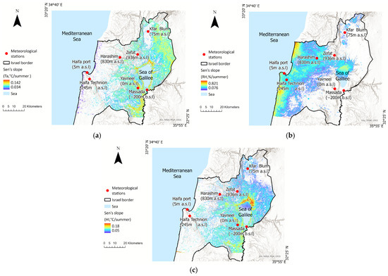
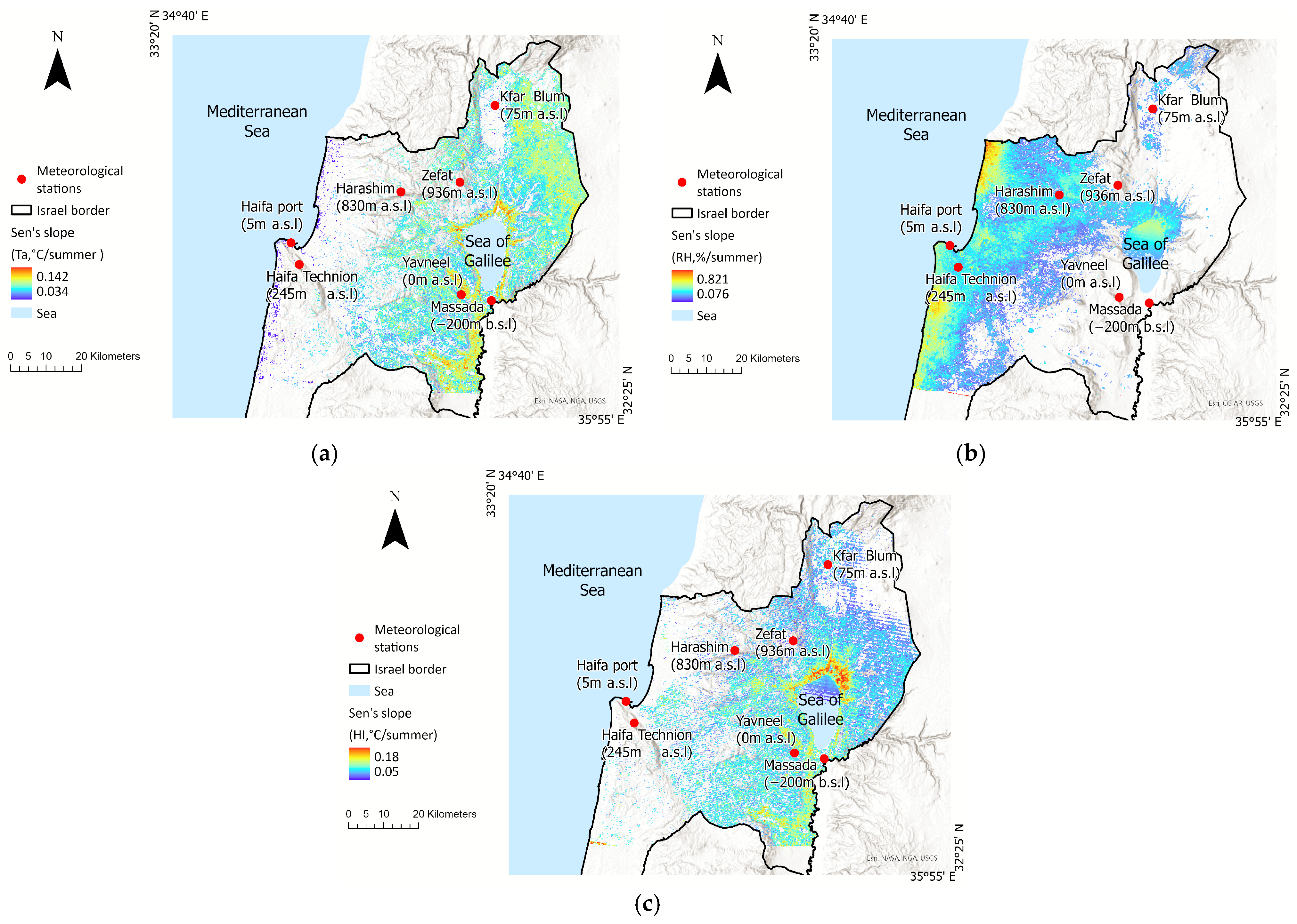
Figure 7 shows spatial pattern changes (sign and strength) in the temporal trends of the different parameters (T_a, RH, HI) over the whole study period, depicting only grid cells that show significant changes (p < 0.05, |z-score| >1.96). The Sen’s slope in grid cells with significant positive temperature change varied between 0.034 and 0.142 °C/summer (Figure 7a), with the most significant air temperature changes occurring in inner regions. Significant RH changes varied from 0.05%/summer to 0.18%/summer (Figure 7b), with the most significant positive changes occurring along the Mediterranean coastline, in accordance with the trend revealed in the in situ measurements at the IMS stations. Significant changes in HI are evident in areas where either significant changes in the ambient temperature or in RH occurred (thus the spatial pattern of the significant HI changes is wider than that of the T_a and RH), ranging between 0.076 °C/summer to 0.821 °C/summer (Figure 7c).

Figure 7. Spatiotemporal changes in the Sen’s slope of summer-average (a) T_a, (b) RH, and (c) HI over four decades, 1984–2024. Only grid cells in which significant changes were found by the Mann-Whitney test are shown (p < 0.05, |z-score| > 1.96).

4. Discussion

Climate change research relies on long-term data that enable the identification and quantification of trends [36]. In this study, two models with moderate spatial resolution (30 m) were developed for examining summer meteorological conditions in EMME over four decades (1984–2024). The models were used to supplement existing, yet spatially sparse, observational data that indicate enhanced regional warming [14]. The complete spatial cover of the T_a and RH estimates enabled the estimation of exposure to severe heat load (HI) at a corresponding spatial resolution. The models’ variables are standard Landsat products (NDVI, emissivity, albedo, LST) and DEM, which are available globally whenever Landsat images are available (since the Landsat thermal channel (TIR) has only been in use since 1984, our study period starts then). Namely, while the models’ structure is not specific to the study area for which they were applied in this work, their calibration against local surface measurements is required.

Previous studies have already found a linear relationship between LST and T_a (e.g., [37,38]) but did not account for many other environmental factors (land-use, land-cover, surface emissivity in the IR wavebands, albedo in the UV–Vis wavebands, climate classification, urban/rural setting) that could affect it. In particular, some urban micro-environments experience increased T_a, a phenomenon termed Urban Heat Island (UHI), with no similar increase in the LST [9,38,39]. Yet, UHI is not caused by only increased T_a, as heat stress may be affected by numerous parameters. Combining LST with surface meteorological observations can provide a more reliable metric for human thermal comfort in urban environments [40,41,42]. In a previous work, we deployed a small-scale sensor network and reported sub-urban spatial variation in HI of 1–4 °C [43]. Future studies should account for additional microenvironment factors, such as local wind speed, distribution of heat sources within the study area, and the topographic slope, and quantify their effects on the HI and UHI [44,45].

A significant challenge in this work was the quality and quantity of Landsat images that could be processed, which varied over the years due to various reasons. (i) The number of available images decreased between 2011 and 2013 due to the transition from the Landsat 5 mission to the Landsat 8 mission (Table S2). (ii) Landsat 7 imagery suffers from a well-documented problem – the presence of unevenly distributed stripes [46]. While the Random Forest model managed to estimate the ambient temperature in the striped areas, visual artifacts often remained evident and complicated further analysis.

The spatial distribution of the IMS meteorological stations affected the accuracy of the models and the propagation of uncertainty throughout the subsequent modeling steps, with the ambient temperature playing a key role in the estimation of the relative humidity, and with these two parameters being central for assessing the heat load. This resulted in higher model errors in sparsely monitored areas and increased the uncertainty in consecutive modeling steps, which was, however, partially balanced by the increase in the number/density of the IMS stations over the years (Figure S2). The use of machine learning (Random Forest, XGBoost, etc.) for estimating the ambient temperature (T_a) from satellite products (NDVI, MDBI, LST) has been reported previously [8,9,11,39], with a typical accuracy of about 2 °C [46,47]. In contrast, models that estimate the ambient relative humidity based on satellite products are less common. Park et al. [16] applied machine learning to predict relative humidity in Japan and South Korea and obtained an RMSE of 10.61%. The accuracy of relative humidity estimation is affected by numerous factors [48], including climate, latitude and longitude of the study area, time of day and other temporal aspects, ambient temperature, topographic slope and turning, land cover, and concentration of airborne particles [16,22,49]. Yet, despite considerable uncertainty, our hybrid model had an error < 8% relative to the in situ RH measurements in 68% of its estimations, better than Park et al. [16].

Typically, trends spanning several decades are assessed on broad spatial scales. In this work, we examined long-term trends at a fine spatial scale (30 m) to enable us to study their spatial patterns. A key challenge in such work is to reveal if a long-term trend exists in records that show considerable variability that is often much larger than the hidden trend [25]. In a previous study [14], using solely surface meteorological observations from 1950 to 2023 across Israel, we found a significant long-term increase of 0.03 °C/summer in summer T_a. Yet, focusing on 2000–2023 (a period that is inadequate for climate change detection as it is <30 years), the long-term slope doubled to 0.06 °C/summer. Here, we report a spatially varied significant positive trend in the observed T_a in northern Israel from the years 1984 to 2024, ranging between 0.04 and 0.06 °C/summer, and a wider spatial variation in a significant positive long-term trend in the modeled T_a, 0.03–0.14 °C/summer. The latter probably reflects the increased uncertainty in areas with sparse IMS stations as well as the plethora of environmental conditions (i.e., micro-environments) devoid of IMS observations. Both the observed and modeled T_a showed a stronger trend in inner regions.

The ambient relative humidity mostly showed no significant trend across the study area (northern Israel) during the summers in the study period (1984–2024), in agreement with a previous study [14] whose study area included the whole of Israel, and which spanned over the summers of 1950–2023, but used only surface IMS meteorological data. In general, the RH is lower in inland areas and higher along the East Mediterranean coast.

While spatial patterns that indicate pronounced climatic shift between 1984 and 2024 can be discerned, coinciding changes in land use that are related to, e.g., population growth (urban sprawl), increasing energy consumption, or even land use (positive) feedback to climate change, significantly affect our capacity to quantify them independently. Strong and clear patterns are observed predominantly in natural areas devoid of, or with minimal impact of, anthropogenic activity. Urban settings, where infrastructure, synthetic materials, and anthropogenic activity amplify the UHI [50], limit our capacity to attribute specific contributions of distinct environmental factors to the observed changes, since the direct anthropogenic contributions dominate the changes.

5. Conclusions

This study demonstrates that spatially discrete climate records can be supplemented by models that use remotely sensed satellite products to obtain a wider picture and enable the tracking of the spatial trends of meteorological parameters at fine-to-moderate spatial resolution. Although originally, Landsat data products were not intended for tracking climate change, the integration of several datasets enables a comprehensive meteorological reconstruction of spatial patterns and temporal trends, which are vital for evaluating climate sensitivity and the vulnerability of communities, ecosystems, and habitats [51]. Climate change is known to carry health implications, e.g., increased morbidity and mortality [52], which is especially relevant for the eastern Mediterranean basin, which is characterized as a hot spot with enhanced warming and severe heat loads [4]. Our findings offer valuable insights for policymakers who are required to address the regional impacts of climate change and to apply climate resilience development (CRD) mechanisms.

References

- Sutton, R.T.; Hawkins, E. ESD Ideas: Global Climate Response Scenarios for IPCC AR6. Earth Syst. Dyn. Discuss. 2020, 11, 751–754. [Google Scholar] [CrossRef] [Scilit]
- Kutiel, H. Climate of Israel. In Landscapes and Landforms of Israel; Frumkin, A., Shtober-Zisu, N., Eds.; World Geomorphological Landscapes; Springer: Cham, Switzerland, 2024; pp. 39–47. [Google Scholar]
- Goldreich, Y. The Climate of Israel: Observation, Research and Application, 1st ed.; Springer: New York, NY, USA, 2003. [Google Scholar]
- Zittis, G.; Almazroui, M.; Alpert, P.; Ciais, P.; Cramer, W.; Dahdal, Y.; Fnais, M.; Francis, D.; Hadjinicolaou, P.; Howari, F.; et al. Climate Change and Weather Extremes in the Eastern Mediterranean and Middle East. Rev. Geophys. 2022, 60, e2021RG000762. [Google Scholar] [CrossRef] [Scilit]
- Orusa, T.; Viani, A.; Moyo, B.; Cammareri, D.; Borgogno-Mondino, E. Risk Assessment of Rising Temperatures Using Landsat 4–9 LST Time Series and Meta® Population Dataset: An Application in Aosta Valley, NW Italy. Remote Sens. 2023, 15, 2348. [Google Scholar] [CrossRef] [Scilit]
- Masson-Delmotteotte, V.; Zhai, P. Regional Trends in Extreme Events in the IPCC 2021 Report. Boletín-Organ. Meteorol. Mund. 2022, 71, 52–62. [Google Scholar]
- Anderson, G.B.; Bell, M.L.; Peng, R.D. Methods to Calculate the Heat Index as an Exposure Metric in Environmental Health Research. Environ. Health Perspect. 2013, 121, 1111–1119. [Google Scholar] [CrossRef] [Scilit] [PubMed]
- Wang, L.; Lu, Y.; Yao, Y. Comparison of Three Algorithms for the Retrieval of Land Surface Temperature from Landsat 8 Images. Sensors 2019, 19, 5049. [Google Scholar] [CrossRef] [Scilit]
- Sun, T.; Sun, R.; Chen, L. The Trend Inconsistency Between Land Surface Temperature and Near Surface Air Temperature in Assessing Urban Heat Island Effects. Remote Sens. 2020, 12, 1271. [Google Scholar] [CrossRef] [Scilit]
- Vanhellemont, Q. Automated Water Surface Temperature Retrieval from Landsat 8/TIRS. Remote Sens. Environ. 2020, 237, 111518. [Google Scholar] [CrossRef] [Scilit]
- Goldblatt, R.; Addas, A.; Crull, D.; Maghrabi, A.; Levin, G.G.; Rubinyi, S. Remotely Sensed Derived Land Surface Temperature (LST) as a Proxy for Air Temperature and Thermal Comfort at a Small Geographical Scale. Land 2021, 10, 410. [Google Scholar] [CrossRef] [Scilit]
- Demarquet, Q.; Rapinel, S.; Gore, O.; Dufour, S.; Hubert-Moy, L. Continuous Change Detection Outperforms Traditional Post-Classification Change Detection for Long-Term Monitoring of Wetlands. Int. J. Appl. Earth Obs. Geoinf. 2024, 133, 104142. [Google Scholar] [CrossRef] [Scilit]
- Fischer, E.M.; Schär, C. Consistent Geographical Patterns of Changes in High-Impact European Heatwaves. Nat. Geosci. 2010, 3, 398–403. [Google Scholar] [CrossRef] [Scilit]
- Shafran-Nathan, R.; Broday, D.M. Long-Term Recurrent Exposure to Excessive Heat in the East Mediterranean and Climate Resilience Development—A Case Study in Israel. Reg. Environ. Change 2024, 24, 153. [Google Scholar] [CrossRef] [Scilit]
- Wulder, M.A.; Roy, D.P.; Radeloff, V.C.; Loveland, T.R.; Anderson, M.C.; Johnson, D.M.; Healey, S.; Zhu, Z.; Scambos, T.A.; Pahlevan, N. Fifty Years of Landsat Science and Impacts. Remote Sens. Environ. 2022, 280, 113195. [Google Scholar] [CrossRef] [Scilit]
- Park, H.; Lee, J.; Yoo, C.; Sim, S.; Im, J. Estimation of Spatially Continuous Near-Surface Relative Humidity over Japan and South Korea. IEEE J. Sel. Top. Appl. Earth Obs. Remote Sens. 2021, 14, 8614–8626. [Google Scholar] [CrossRef] [Scilit]
- Liao, Q.-Y.; Leng, P.; Li, Z.-L.; Ren, C.; Sun, Y.-Y.; Gao, M.-F.; Duan, S.-B.; Shang, G.-F. A Method for Deriving Relative Humidity from Modis Data under All-Sky Conditions. IEEE Trans. Geosci. Remote Sens. 2020, 59, 8992–9006. [Google Scholar] [CrossRef] [Scilit]
- Song, K.; Hsu, A.; Peng, W.; Yu, Y.; Kittner, N. Projecting Future Heat Stress Disparities to 2100 in the Contiguous United States. Res. Sq. 2023. [Google Scholar] [CrossRef] [Scilit]
- Yao, Y.; Lu, L.; Guo, J.; Zhang, S.; Cheng, J.; Tariq, A.; Liang, D.; Hu, Y.; Li, Q. Spatially Explicit Assessments of Heat-Related Health Risks: A Literature Review. Remote Sens. 2024, 16, 4500. [Google Scholar] [CrossRef] [Scilit]
- Israeli Meteorological Service. Available online: https://ims.gov.il/en (accessed on 14 January 2026).
- Yosef, Y.; Aguilar, E.; Alpert, P. Changes in Extreme Temperature and Precipitation Indices: Using an Innovative Daily Homogenized Database in Israel. Int. J. Climatol. 2019, 39, 5022–5045. [Google Scholar] [CrossRef] [Scilit]
- Halfon, N.; Osetinsky-Tzidaki, I.; Vadislavsky, E. Mapping Israel’s Daily Minimum Temperature: Applying Remote Sensing Data in Spatial Regression Equations; Research Report No. 4000-0804-2020-0000086; Israel Meteorological Service: Bet Dagan, Israel, 2020. [Google Scholar]
- Reis, M.S.; de Barros, L.S.; Rodrigues Neto, M.R.; de Moraes, D.R.V.; Moreira, N.A.P.; Alves, G.M.R.; Adorno, B.V.; Messias, C.G.; Dutra, L.V.; Rennó, C.D. Assessing Interpreter’s Disagreements in Land Cover Reference Data Collection from Historical Landsat Time Series in Amazon. Int. J. Remote Sens. 2024, 45, 5192–5223. [Google Scholar] [CrossRef] [Scilit]
- U.S. Geological Service Landsat Collection 1. Available online: https://www.usgs.gov/landsat-missions/landsat-collection-1 (accessed on 14 January 2026).
- Vogelmann, J.E.; Gallant, A.L.; Shi, H.; Zhu, Z. Perspectives on Monitoring Gradual Change Across the Continuity of Landsat Sensors Using Time-Series Data. Remote Sens. Environ. 2016, 185, 258–270. [Google Scholar] [CrossRef] [Scilit]
- Missions, L. Landsat 7 (L7) Data Users Handbook (May 2024); Version 3.0; Department of the Interior U.S. Geological Survey: Reston, VA, USA, 2024. [Google Scholar]
- Missions, L. Landsat 8 (L8) Data Users Handbook (November 2019); Version 5.0; Department of the Interior U.S. Geological Survey: Reston, VA, USA, 2019. [Google Scholar]
- U.S. Geological Survey. The USGS Global Visualization Viewer (GloVis). Available online: https://glovis.usgs.gov/ (accessed on 14 January 2026).
- Sekertekin, A.; Bonafoni, S. Land Surface Temperature Retrieval from Landsat 5, 7, and 8 over Rural Areas: Assessment of Different Retrieval Algorithms and Emissivity Models and Toolbox Implementation. Remote Sens. 2020, 12, 294. [Google Scholar] [CrossRef] [Scilit]
- Flückiger, B.; Kloog, I.; Ragettli, M.S.; Eeftens, M.; Röösli, M.; de Hoogh, K. Modelling Daily Air Temperature at a Fine Spatial Resolution Dealing with Challenging Meteorological Phenomena and Topography in Switzerland. Int. J. Climatol. 2022, 42, 6413–6428. [Google Scholar] [CrossRef] [Scilit]
- He, T.; Liang, S.; Wang, D.; Cao, Y.; Gao, F.; Yu, Y.; Feng, M. Evaluating Land Surface Albedo Estimation from Landsat MSS, TM, ETM+, and OLI Data Based on the Unified Direct Estimation Approach. Remote Sens. Environ. 2018, 204, 181–196. [Google Scholar] [CrossRef] [Scilit]
- Breiman, L. Random Forests. Mach. Learn. 2001, 45, 5–32. [Google Scholar] [CrossRef] [Scilit]
- Bolton, D. The Computation of Equivalent Potential Temperature. Mon. Weather Rev. 1980, 108, 1046–1053. [Google Scholar] [CrossRef] [Scilit]
- Cook, M.J. Atmospheric Compensation for a Landsat Land Surface Temperature Product; Rochester Institute of Technology: Henrietta, NY, USA, 2014. [Google Scholar]
- Peng, G.; Li, J.; Chen, Y.; Norizan, A.P.; Tay, L. High-Resolution Surface Relative Humidity Computation Using MODIS Image in Peninsular Malaysia. Chin. Geogr. Sci. 2006, 16, 260–264. [Google Scholar] [CrossRef] [Scilit]
- McMichael, A.J. Globalization, Climate Change, and Human Health. N. Engl. J. Med. 2013, 368, 1335–1343. [Google Scholar] [CrossRef] [Scilit]
- Mutiibwa, D.; Strachan, S.; Albright, T. Land Surface Temperature and Surface Air Temperature in Complex Terrain. IEEE J. Sel. Top. Appl. Earth Obs. Remote Sens. 2015, 8, 4762–4774. [Google Scholar] [CrossRef] [Scilit]
- Rosas, J.; Houborg, R.; McCabe, M.F. Sensitivity of Landsat 8 Surface Temperature Estimates to Atmospheric Profile Data: A Study Using MODTRAN in Dryland Irrigated Systems. Remote Sens. 2017, 9, 988. [Google Scholar] [CrossRef] [Scilit]
- do Nascimento, A.C.L.; Galvani, E.; Gobo, J.P.A.; Wollmann, C.A. Comparison between Air Temperature and Land Surface Temperature for the City of São Paulo, Brazil. Atmosphere 2022, 13, 491. [Google Scholar] [CrossRef] [Scilit]
- Marquez-Torres, A.; Kumar, S.; Aznarez, C.; Jenerette, G.D. Assessing the Cooling Potential of Green and Blue Infrastructure from Twelve US Cities with Contrasting Climate Conditions. Urban For. Urban Green. 2025, 104, 128660. [Google Scholar] [CrossRef] [Scilit]
- Chen, L.; Zhang, Y.; Zhu, E.; Che, Y.; Wu, Y. Segregation of Sea Breezes and Cooling Effects on Land-Surface Temperatures in a Coastal City. Sustain. Cities Soc. 2025, 118, 106017. [Google Scholar] [CrossRef] [Scilit]
- Shi, D.; Song, J.; Huang, X.; Chan, P.W. Modelling and Optimization of Urban Green-Blue Infrastructure Design for City Cooling. Build. Environ. 2025, 279, 113096. [Google Scholar] [CrossRef] [Scilit]
- Shafran-Nathan, R.; Broday, D.M. Spatiotemporal Variability in Exposure to Excessive Heat at the Sub-Urban Scale. Clim. Change 2022, 174, 7. [Google Scholar] [CrossRef] [Scilit]
- Cheung, P.K.; Jim, C.Y.; Hung, P.L. Preliminary Study on the Temperature Relationship at Remotely-Sensed Tree Canopy and below-Canopy Air and Ground Surface. Build. Environ. 2021, 204, 108169. [Google Scholar] [CrossRef] [Scilit]
- Arunab, K.S.; Mathew, A. Impact of Planned Urban Development on Urban Heat Island Effect: Resilient Cities for a Sustainable Future. Environ. Sci. Pollut. Res. 2025, 1–37. [Google Scholar] [CrossRef] [Scilit] [PubMed]
- Adıyaman, H.; Emre Varul, Y.; Bakırman, T.; Bayram, B. Stripe Error Correction for Landsat-7 Using Deep Learning. PFG–J. Photogramm. Remote Sens. Geoinf. Sci. 2025, 93, 51–63. [Google Scholar] [CrossRef] [Scilit]
- Pelta, R.; Chudnovsky, A.A.; Schwartz, J. Spatio-Temporal Behavior of Brightness Temperature in Tel-Aviv and Its Application to Air Temperature Monitoring. Environ. Pollut. 2016, 208, 153–160. [Google Scholar] [CrossRef] [Scilit]
- Cristóbal, J.; Ninyerola, M.; Pons, X. Modeling Air Temperature Through a Combination of Remote Sensing and GIS Data. J. Geophys. Res. Atmos. 2008, 113. [Google Scholar] [CrossRef] [Scilit]
- Stohl, A. Computation, Accuracy and Applications of Trajectories—A Review and Bibliography. Atmos. Environ. 1998, 32, 947–966. [Google Scholar] [CrossRef] [Scilit]
- Zhang, W.; Li, J.; Xu, S.; Zhao, Y.; Jian, B. Spatio-Temporal Variation of Critical Relative Humidity Based on Multiple Datasets. Remote Sens. 2023, 15, 4187. [Google Scholar] [CrossRef] [Scilit]
- Pelta, R.; Chudnovsky, A.A. Spatiotemporal Estimation of Air Temperature Patterns at the Street Level Using High Resolution Satellite Imagery. Sci. Total Environ. 2017, 579, 675–684. [Google Scholar] [CrossRef] [Scilit] [PubMed]
- Watts, N.; Amann, M.; Arnell, N.; Ayeb-Karlsson, S.; Beagley, J.; Belesova, K.; Boykoff, M.; Byass, P.; Cai, W.; Campbell-Lendrum, D. The 2020 Report of The Lancet Countdown on Health and Climate Change: Responding to Converging Crises. Lancet 2021, 397, 129–170. [Google Scholar] [CrossRef] [Scilit] [PubMed]
Disclaimer/Publisher’s Note: The statements, opinions and data contained in all publications are solely those of the individual author(s) and contributor(s) and not of MDPI and/or the editor(s). MDPI and/or the editor(s) disclaim responsibility for any injury to people or property resulting from any ideas, methods, instructions or products referred to in the content. |
© 2026 by the authors. Licensee MDPI, Basel, Switzerland. This article is an open access article distributed under the terms and conditions of the Creative Commons Attribution (CC BY) license.