Seasonal Amplification and Spatial Reorganization of Atmospheric Ammonia (NH₃) in Northeast China

Abstract

Regional assessments of atmospheric ammonia must distinguish changes in annual abundance from changes in seasonality and hotspot organization. We analyzed monthly Infrared Atmospheric Sounding Interferometer (IASI) total columns over Liaoning, Jilin and Heilongjiang during 2008–2024 on a 0.2° grid. We constructed a Unified Spatiotemporal Bayesian Additive Regression Trees model (UST-BART) for 2008–2022 using nonnegative complete observations, combining location means and within-location departures with geographical and calendar backgrounds. Regional columns increased at 4.52 × 10⁻⁵ mol m⁻² decade⁻¹, and positive trends covered 93.6% of represented area. The seasonal amplitude of atmospheric NH₃ columns increased by 119.7% between 2008–2012 and 2019–2024; relative hotspots remained concentrated in Liaoning, with southwestward centroid trends despite start-year-sensitive endpoint distances (477.4 vs. 46.8 km). Liaoning retained the largest absolute seasonal cycle, whereas Heilongjiang showed the largest proportional provincial amplification. UST-BART identified a positive temperature association, a U-shaped soil-moisture association and a broadly inverse-U association with boundary layer height. Temperature contrasts varied jointly with moisture and boundary layer conditions, with the largest provincial temperature response in Liaoning. Temporal and spatial holdouts yielded R² values of 0.414 and 0.286. These findings reveal strengthening seasonality and spatial reorganization of NH₃, with context-dependent environmental associations that support regionally focused monitoring.

1. Introduction

Atmospheric ammonia (NH₃) connects agricultural nitrogen losses with secondary aerosol formation and nitrogen deposition. Livestock waste and fertilizer application are its principal sources in China [1]. Nationwide measurements documented rising nitrogen deposition, with ammonium dominating bulk deposition and changes evident in ecosystem nitrogen uptake [2]. The atmospheric consequences depend on the supply of other precursors: chemical transport modelling showed that sulfate–nitrate–ammonium aerosol responses to emission controls vary across Chinese regions [3]. NH₃ abatement can reduce particulate pollution and deposition while aggravating precipitation acidification under some scenarios [4]. Its estimated societal benefits nevertheless substantially exceed agricultural mitigation costs [5]. Assessing regional NH₃ therefore requires both a description of its changing atmospheric distribution and an account of the conditions accompanying that change. Historical inventories show marked seasonal differences in Chinese agricultural emissions [6]. Improved fertilizer calendars and rice-cropland allocation have strengthened agreement between inventories and observations [7]. Global cropland estimates likewise reveal substantial variation among crops and fertilization practices [8]. These findings establish agricultural context, although annual inventories alone cannot resolve the timing of monthly emission peaks.

Satellite observations provide regional coverage beyond individual monitoring sites. Early Infrared Atmospheric Sounding Interferometer (IASI) measurements resolved agricultural and biomass-burning hotspots [9]. Subsequent retrieval development supplied multiyear total-column records with explicit error characterization [10]. Neural-network methods improved conversion of infrared measurements to NH₃ columns [11]. Reanalysis-based retrievals addressed discontinuities in operational meteorological inputs [12]. The version 4 product further improved consistency across time and instruments [13]. Such records have revealed increasing columns in East Asia and other major source regions during 2008–2018 [14]. An independent Atmospheric Infrared Sounder analysis associated agricultural-region increases with changing chemical loss, temperature and agricultural activity [15]. IASI has also exposed industrial and agricultural point sources underestimated in inventories [16]. Wind-informed CrIS and IASI analyses can estimate point-source emissions and atmospheric lifetimes when additional plume information is available [17]. At the pixel scale, validation against aircraft and surface profiles emphasizes the importance of close spatial and temporal matching [18]. Thus, the long record supports analysis of regional trends and recurrent hotspots, while their interpretation still depends on atmospheric processing and observational support.

A rising NH₃ column need not indicate a proportional rise in emissions. Chinese SO₂ and NO_x emissions fell substantially during 2010–2017, whereas estimated NH₃ emissions remained approximately stable [19]. Observations and model experiments over the North China Plain linked reduced sulfate formation to increasing gaseous NH₃ despite slightly declining NH₃ emissions [20]. Simulations for eastern China found that acid-precursor reductions could explain much of the observed column increase during 2011–2015 [21]. Global inversions also demonstrate the importance of accounting for changing SO₂ when estimating NH₃ emission trends [22]. Satellite-constrained NH₃ fluxes have improved chemical transport model agreement with atmospheric measurements [23]. Meteorology adds another influence: a United States study attributed more simulated interannual surface-NH₃ variability to weather than to changing acid-precursor emissions during 2008–2012 [24]. Long-term measurements in urban Beijing found that surface, satellite and inventory trends could diverge, with temperature and moisture relationships depending on the timescale examined [25]. Temperature, soil moisture and boundary layer height (BLH) should therefore be examined jointly rather than summarized by isolated regional correlations.

For Northeast China, existing national analyses establish the broad NH₃ context but leave the regional organization of change less resolved. Historical work combined inventories, satellite observations and transport modelling to characterize Chinese NH₃ and NO₂ evolution [26]. A more recent assessment using CrIS, ground measurements, chemical transport modelling and random forests reported increasing NH₃ concentrations over its Northeast China Plain subregion [27]. Geostationary measurements further show that seasonal peak timing differs geographically across East Asia [28]. Here we focus on Liaoning, Jilin and Heilongjiang, collectively NE3, asking whether the longer record reveals amplification of the high-column season, persistence or redistribution of hotspots, and provincial differences in environmental response.

These questions require separating persistent differences among locations from changes at the same location. The distinction between unit means and within-unit departures is established in longitudinal modelling [29]. We use it to construct a Unified Spatiotemporal Bayesian Additive Regression Trees model (UST-BART), combining each dynamic driver’s location mean and temporal departure with static cropland and geographical and calendar backgrounds. BART supplies a regularized sum-of-trees response capable of nonlinear relationships and interactions [30]. Estimation uses the existing accelerated XBART procedure [31]. Unlike BART using undecomposed predictors, UST-BART explicitly represents between-location backgrounds and within-location departures, allowing their nonlinear associations and interactions to be examined within one shared response function. Accumulated local effects (ALE) summarize that function while limiting unsupported extrapolation under correlated predictors [32]. Provincial curves and supported local interaction contrasts then reveal how its response varies across observed environmental contexts.

We analyze monthly IASI columns over 2008–2024 on a common 0.2° grid, linking trends, seasonal amplitude and hotspot organization. UST-BART covers 2008–2022, the period supported by the emission inventories. Separate temporal and spatial holdouts follow the principle that validation for structured data should reflect the intended prediction setting [33]. This combination allows regional NH₃ evolution and environmental associations to be assessed within the same study domain.

2. Methods

2.1. Study Area and Datasets

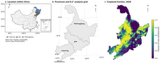
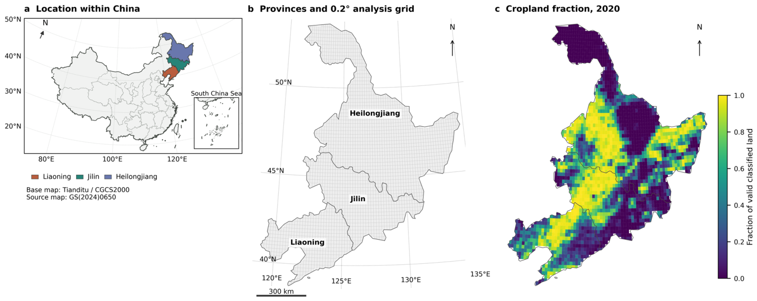
The NE3 domain comprises 2278 globally anchored 0.2° cells whose centres lie inside the union of Liaoning, Jilin and Heilongjiang (Figure 1). The descriptive record spans January 2008–December 2024; model analysis ends in 2022 because the supplied EDGAR inventories end in that year. Monthly NH₃ total columns were taken from the ESA CCI ULB–LATMOS version 4.0.1R MERGED Level-3 AM+PM product [34]. Its retrieval framework is described by Clarisse et al. [13]. We retained the source 0.2° coordinates and selected nh3_total_column_ampm in mol m⁻², together with random uncertainty, systematic uncertainty and fractional observation support. Monthly source identities indicate Metop-A for 2008–2013, Metop-B for 2014–2019 and Metop-C for 2020–2024. The full record and retrieval diagnostics are given in Figures S1 and S2.

Figure 1. Study area and analytical grid. (a) NE3 within China, using Tianditu provincial and boundary linework distributed by GeoJSON.CN v0.3.0 (source map GS(2024)0650, CGCS2000). The locator uses Lambert conformal conic projection (25° N/47° N, 105° E); the inset shows all nine southern discontinuous segments, while northern South China Sea and east-Taiwan segments remain in the main locator. (b) Provincial boundaries and centre-selected 0.2° cells clipped to NE3. (c) Static 2020 cropland fraction of valid classified land. Panels (b,c) use geoBoundaries ADM1 (2019, revision 9469f09) and WGS84 Lambert conformal conic projection (40° N/52° N, 126° E). The 300 km scale applies to NE3 panels; unsupported land cells are unfilled.

Because the earlier product guide favours AM over land and recommends a support filter for long-period means, we also extracted AM from all 204 monthly source files [35]. Regional and provincial trends, seasonal amplitudes and negative-retrieval fractions were repeated for AM and AM+PM, with and without fractional support ≥ 0.25 (Figure S3; Table S1). This field is dimensionless. The supplied AM+PM record was retained for the main analysis, with observational sensitivities evaluated separately from model responses.

Meteorological predictors comprised two-metre air temperature and BLH from monthly ERA5 data at 0.25° [36]. Soil moisture came from ERA5-Land layer 1 (0–7 cm) at 0.1° [37]. Temperature was converted to °C; BLH and soil moisture retained units of m and m³ m⁻³. EDGAR v8.1 FT2022 AP supplied annual 0.1° NH₃ Agricultural soils (AGS) and Manure management (MNM) emissions, together with total SO₂ and NO_x emissions [38]. We conservatively aggregated source cell masses and converted them to kg km⁻² yr⁻¹, preserving species definitions; each annual emission density was repeated across the corresponding twelve monthly records to align with monthly IASI NH₃ and meteorological predictors, without implying an observed monthly emission profile. Static cropland was derived from the 2020 MCD12Q1.061 LC_Type1 and QC layers, supplied through AppEEARS at nominal 500 m resolution [39]. It comprises IGBP class 12 as a fraction of valid classified land; class 14 mosaics were excluded. Provincial boundaries use geoBoundaries gbOpen CHN ADM1, reference year 2019 [40]. Table 1 summarizes data support and model roles, with annual coverage in Table S2.

Table 1. Datasets and analytical support.

Variable	Source	Support	Unit	Role
IASI NH3	ESA CCI 4.0.1R MERGED AM+PM	0.2°; monthly, 2008–2024	mol m−2	Response; mechanisms through 2022
T2m	ERA5 monthly means	0.25°; monthly, 2008–2024	°C	Between and within
Soil moisture	ERA5-Land layer 1, 0–7 cm	0.1°; monthly, 2008–2024	m3 m−3	Between and within
BLH	ERA5 monthly means	0.25°; monthly, 2008–2024	m	Between and within
NH3-AGS	EDGAR v8.1 FT2022 AP Agricultural soils	0.1°; annual, 2008–2022	kg km−2 yr−1	Between and annual within
NH3-MNM	EDGAR v8.1 FT2022 AP Manure management	0.1°; annual, 2008–2022	kg km−2 yr−1	Between and annual within
SO2	EDGAR v8.1 FT2022 AP TOTALS	0.1°; annual, 2008–2022	kg km−2 yr−1	Between and annual within
NOx	EDGAR v8.1 FT2022 AP TOTALS	0.1°; annual, 2008–2022	kg km−2 yr−1	Between and annual within
Cropland	MCD12Q1.061 LC_Type1 + QC, 2020	Nominal 500 m; static 2020 layer	1	Between only

Fields share the 0.2° grid. Annual inventories repeat within each year; cropland is static. Model NH₃ total columns use μmol m⁻² (10⁶ times source units). Retrieval uncertainty and fractional support are observational diagnostics.

2.2. Data Harmonization and Panel Construction

All fields were indexed to a stable 0.2° cell identifier and calendar month. Actual cell intersections with NE3 and each province were calculated in EPSG:6933 and supplied the area weights; the province with the largest overlap supplied the categorical model label. Maps show cells clipped to the administrative union in WGS84 Lambert conformal conic projection (40° N and 52° N standard parallels, 126° E central meridian). The regional monthly mean in Equation (1) uses overlap area a_i and a finite-response indicator v_it, so missing observations contribute to neither numerator nor denominator. Regional annual means average the twelve monthly regional means. Cell annual means use available retrievals: all 38,726 cell-years have 9–12 valid months. A sensitivity reverses this aggregation order by averaging within cells first (Table S3).

$${\overline{Y}}_t={\displaystyle \frac{{\displaystyle {\sum }_{i=1}^n}{a}_i v_{\mathit{it}} Y_{\mathit{it}}}{{\displaystyle {\sum }_{i=1}^n}{a}_i v_{\mathit{it}}}}$$

(1)

IASI values already occupied the target grid and were preserved after correcting coordinate roundoff. ERA5 temperature and BLH used bilinear interpolation; ERA5-Land soil moisture used spherical source–target overlap areas over finite support. Missing land support was not filled. EDGAR source masses were redistributed according to overlap fractions, checked against direct source sums, and divided by whole target-cell area a_iᵍ to obtain annual density E_iᵧ from aggregated mass M_iᵧ in kilograms. Cropland fraction C_i used exact pixel–cell intersections in EPSG:6933, as defined in Equation (2).

$$C_i={\displaystyle \frac{a_{i,\mathit{crop}}}{a_{i,\mathit{valid} \mathit{land}}}}, E_{\mathit{iy}}={\displaystyle \frac{M_{\mathit{iy}}}{a_i^g}}$$

(2)

For cropland, valid IGBP classes 1–16 required QC codes 0, 5, 8 or 9. Unclassified land, water-related labels and fill were excluded. Zero cropland on valid land remained zero; absent valid land support remained missing. The supplied geographic AppEEARS raster was integrated by area intersection without further resampling or imputation. Descriptive NH₃ summaries retained all finite retrievals, including negative values. Although negative retrievals do not represent physically negative columns, they can occur under low-signal retrieval conditions. Model analysis set negative NH₃ to NaN and used complete records, without filling, truncation to zero or logarithmic transformation. Of 410,040 candidate cell-months in 2008–2022, 54,829 (13.4%) negative responses and 672 other incomplete records were excluded, leaving 354,539 observations at 2276 locations. Because excluded negative retrievals were concentrated in low-column conditions, the selected modelling sample was shifted toward higher NH₃ columns. Two Heilongjiang cells lacked cropland support throughout. Model responses were converted to μmol m⁻². Exclusions and matched observation/subset comparisons are documented in Figure S4 and Table S4; predictor distributions appear in Figure S5 and Table S5.

2.3. Trends, Seasonality and Hotspot Analysis

Annual regional, provincial and cell trends over 2008–2024 were estimated with Theil–Sen slopes and 95% confidence intervals, reported per decade [41]. Regional and provincial sensitivities used ordinary least-squares regression with heteroskedasticity- and autocorrelation-consistent (HAC) standard errors, one annual lag and a two-lag check, finite-sample correction and t-based inference [42]. Cell evidence used two-sided, continuity-corrected Mann–Kendall tests with tie correction [43]. Benjamini–Hochberg false discovery rate adjustment across finite cell tests defined increasing and decreasing categories at q < 0.05 [44]. Their prevalence uses administrative overlap area. Because cell-level tests do not adjust for autocorrelation, we additionally used two- and three-year circular moving-block bootstrap to assess regional trend uncertainty and field-wide significance, with shared temporal blocks across cells (Tables S3 and S6).

Seasonality was summarized for Early (2008–2012), Middle (2013–2018) and Late (2019–2024). Equation (3) defines monthly cell climatology C_im and peak-to-trough amplitude 𝒜_i, using available observations within each period. Regional climatologies were calculated from the area-weighted monthly series; annual regional amplitudes use each year’s twelve monthly means. Two sensitivities compare June–August with December–February and fit the first annual harmonic to the twelve climatological values. Percentage amplification uses Early amplitude as denominator, and the spatial increase fraction uses positive Late-minus-Early cell differences (Figure S6; Table S7). Instrument-transition sensitivity used contemporaneous Metop-A/B (2014) and Metop-B/C (2020) observations, same-instrument bridging, season-adjusted change-point tests, instrument-specific trends and amplitudes, and monthly overlap-offset scenarios (Table S8).

$$\begin{array}{c}{C}_{\mathit{im}}^{\left(P\right)}={\displaystyle \frac{1}{N_{\mathit{im}}^{\left(P\right)}}}\hfill \\ {\mathcal{A}}_i^{\left(P\right)}=\underset{m}{\max } C_{\mathit{im}}^{\left(P\right)}-\underset{m}{\min } C_{\mathit{im}}^{\left(P\right)}\hfill \\ {\mathcal{A}}_{\mathit{JJA}-\mathit{DJF}}={\overline{Y}}_{\mathit{JJA}}-{\overline{Y}}_{\mathit{DJF}}\hfill \\ C_m=\kappa +a \sin \left({\displaystyle \frac{2\mathit{\pi m}}{12}}\right)+b \cos \left({\displaystyle \frac{2\mathit{\pi m}}{12}}\right)+e_m, {\mathcal{A}}_H=2\sqrt{a^2+b^2}\hfill \end{array}$$

(3)

Annual hotspots strictly exceed the area-weighted P90 of annual cell columns (Equation (4)). The weighted inverse empirical-distribution quantile retains ties, so realized hotspot area need not be exactly 10%. Persistence P_i is the fraction of seventeen years classified as a hotspot; persistent cells require at least fourteen hotspot years. Period frequency uses the corresponding Early, Middle or Late denominator.

$$\begin{array}{c}{q}_{0.90,y}=Q_{0.90}^{\left(w\right)}\left(\left\{Y_{\mathit{iy}}\right\}; \left\{a_i\right\}\right), H_{\mathit{iy}}=1\left(Y_{\mathit{iy}}>q_{0.90,y}\right)\hfill \\ P_i={\displaystyle \frac{1}{17}}{\displaystyle {\sum }_{y=2008}^{2024}}{H}_{\mathit{iy}}\hfill \end{array}$$

(4)

An excess-weighted centroid and area-weighted adjacent-year Jaccard similarity summarize hotspot reorganization (Equation (5)). Centroids use cell-centre coordinates x_i in EPSG:6933, overlap area and positive NH₃ excess above the annual threshold; endpoint displacement is a WGS84 geodesic. Provincial fractions use each province’s represented area. Sensitivities include annual P80/P95 and a fixed P90 of full-period cell means (Figure S7; Table S9). We further estimated centroid-coordinate trends using Theil–Sen slopes and moving-block bootstrap confidence intervals, including a sensitivity analysis excluding 2008 (Table S10).

$$\begin{array}{c}{c}_y={\displaystyle \frac{{\sum }_i{a}_i \max \left(Y_{\mathit{iy}}-q_{0.90,y}, 0\right) x_i}{{\sum }_i{a}_i \max \left(Y_{\mathit{iy}}-q_{0.90,y}, 0\right)}}\\ J_y={\displaystyle \frac{A\left(H_y \cap H_{y+1}\right)}{A\left(H_y \cup H_{y+1}\right)}}\end{array}$$

(5)

2.4. Construction of Ust-Bart

We constructed UST-BART to distinguish environmental associations with persistent spatial conditions from those with temporal departures while allowing them to interact in one fitted response. Each dynamic driver enters as its location mean X_iᴮ and within-location departure X_itᵂ, following the established distinction between unit means and within-unit deviations [29]. Equation (6) calculates means from finite covariate histories before response exclusions. Full-data and spatial-validation fits use 2008–2022 histories. Temporal validation uses only 2008–2018 means, which are retained when constructing later test departures. Meteorological departures include seasonal and interannual variation; they are not same-month climate anomalies. Inventory departures vary annually. Seven dynamic drivers supply fourteen components, and static cropland adds a between component.

$$\begin{array}{c}{\overline{X}}_i={\displaystyle \frac{1}{T_i}}{\sum }_{t\in {\mathcal{T}}_{\mathrm{i}}}{X}_{\mathit{it}}, X_i^B={\overline{X}}_i, X_{\mathit{it}}^W=X_{\mathit{it}}-{\overline{X}}_i\hfill \\ X_{\mathit{it}}=X_i^B+X_{\mathit{it}}^W\hfill \end{array}$$

(6)

These fifteen physical components enter a shared BART sum-of-trees function with background vector Z_it (Equation (7)) [30]. T_k and M_k denote tree partitions and terminal responses, and ε_it is Gaussian observation error on the untransformed response scale. The ten background columns comprise longitude, latitude, three binary province indicators passed as ordered categorical variables, year centred on 2015, and first and second annual sine–cosine harmonics. The resulting 25-column model represents geographical and calendar context through the forest rather than an explicit spatial covariance process. ALE, interaction and provincial summaries all evaluate this same function in observed reference contexts (Figure S8).

$$\begin{array}{c}{Y}_{\mathit{it}}=F_{\mathrm{UST}-\mathrm{BART}}\left(X_i^B, X_{\mathit{it}}^W, Z_{\mathit{it}}\right)+{\epsilon }_{\mathit{it}}, {\epsilon }_{\mathit{it}} \sim N\left(0, {\sigma }^2\right)\hfill \\ F_{\mathrm{UST}-\mathrm{BART}}\left(X\right)={\displaystyle {\sum }_{k=1}^K}{g}_k\left(X; T_k, M_k\right), K=100\hfill \end{array}$$

(7)

UST-BART was estimated with the established XBART grow-from-root (GFR) procedure [31]. We used StochTree 0.4.5 [45]. Fits used 100 trees, 80 GFR sweeps, α = 0.95, β = 2, maximum depth 6, minimum leaf size 20 and a cutpoint grid of 100. After discarding the first 30 sweeps, 50 forests per seed were retained from seeds 20261004 and 20261005. The call used num_gfr = 80, num_burnin = 0 and num_mcmc = 0, with four threads. Estimation therefore consists of standalone GFR fitting. On the internally standardized response scale, leaf means have zero-centred Gaussian priors; their variance uses inverse-gamma shape 3, scale Var(y*)/100 = 0.01 and initialization 0.01. The default global error-variance prior has inverse-gamma shape and scale zero, corresponding to the limiting 1/σ² prior. Predictions restore the training mean and population standard deviation. Table S11 records the full configuration and installed defaults.

2.5. Response Curves Interactions and Provincial Comparisons

Physical-driver relevance was calculated from split use in each retained forest (Equation (8)). N_j⁽ˢ⁾ is the split count for physical component j in forest s; normalization includes only physical components $𝒫$, excluding the ten background columns. Overall driver relevance sums its between and within shares, averaged equally over retained forests (Table S12). These shares describe model partitioning, not explained variance or causal contributions.

$$R_j^{\left(s\right)}={\displaystyle \frac{N_j^{\left(s\right)}}{{\sum }_{k\in \mathcal{P}}{N}_k^{\left(s\right)}}}, R_j={\displaystyle \frac{1}{S}}{\displaystyle {\sum }_{s=1}^S}{R}_j^{\left(s\right)}, R_X=R_{X^B}+R_{X^W}$$

(8)

First-order ALE follows the local-effect construction of Apley and Zhu [32]. For each bin, Equation (9) averages prediction differences between its endpoints over observed reference rows 𝓡_jᵦ, holding other variables at their observed values. Differences are accumulated, adjusted by half the current-bin step to evaluate the midpoint cᵦ, and centred by their observed-bin-frequency mean κ_j^(s). Curves use up to twenty quantile bins over P5–P95 and at most 96 reference rows per bin; density strips show observations per predictor width.

$$\begin{array}{c}{\delta }_{\mathit{jb}}^{\left(s\right)}={\displaystyle \frac{1}{\left|{\mathcal{R}}_{\mathit{jb}}\right|}}{\sum }_{r\in {\mathcal{R}}_{j\beta }}\left[F_s\left(z_b, X_{-j,r}\right)-F_s\left(z_{b-1}, X_{-j,r}\right)\right]\hfill \\ f_j^{\left(s\right)}\left(c_b\right)={\displaystyle {\sum }_{\mathcal{l}=1}^b}{\delta }_{j\mathcal{l}}^{\left(s\right)}-{\displaystyle \frac{1}{2}}{\delta }_{\mathit{jb}}^{\left(s\right)}-{\kappa }_j^{\left(s\right)}, c_b={\displaystyle \frac{z_{b-1}+z_b}{2}}\hfill \end{array}$$

(9)

We compared endpoint direction, local slope signs, major turns and cross-seed shape correlation. Stable curves require r ≥ 0.90, matching endpoint direction and major turning pattern, and ≥80% slope-sign agreement; r < 0.80 is unstable. Major turns require prominence ≥ 20% of curve amplitude and two-bin separation, with cross-seed positions compared within 15% of grid length (Figures S9 and S10; Table S13). All 105 pairs of physical components were screened using within-tree co-occurrence and supported local contrasts. Equation (10) gives their four-corner mixed finite difference, averaged over observed contexts. Each surface uses a 5 × 5 quantile grid over P5–P95. Rectangles require at least fifty rows and ten locations; up to twenty-four locations provide one sampled reference row each, shared between seeds. Equation (11) weights RMS interaction strength by observed rectangle frequency. These are local contrasts rather than cumulative second-order ALE (Figures S11 and S12; Table S14).

$$\begin{array}{c}{G}_{\mathit{ab}}^{\left(s\right)}\left(u, v\right)={\displaystyle \frac{1}{\left|{\mathcal{R}}_{\mathit{ab}}\right|}}{\sum }_{r\in {\mathcal{R}}_{\alpha \beta }}{F}_s\left(u, v, X_{-\mathit{ab},r}\right)\hfill \\ I_{\mathit{ab}}^{\left(s\right)}=G_{\mathit{ab}}^{\left(s\right)}\left(x_a^H, x_b^H\right)-G_{\mathit{ab}}^{\left(s\right)}\left(x_a^H, x_b^L\right)\hfill \\ -G_{\mathit{ab}}^{\left(s\right)}\left(x_a^L, x_b^H\right)+G_{\mathit{ab}}^{\left(s\right)}\left(x_a^L, x_b^L\right)\hfill \end{array}$$

(10)

$${\mathrm{RMS}}_{\mathit{ab}}=\sqrt{{\sum }_{c\in {\mathcal{C}}_{\alpha \beta }}{w}_c {\overline{I}}_{\mathit{ab},c}^2}, {\sum }_{c\in {\mathcal{C}}_{\alpha \beta }}{w}_c=1$$

(11)

Provincial ALE curves use the same forests with reference rows restricted to each province, at most seventy-two per bin. Direct comparisons use the intersection of provincial P5–P95 ranges and independently centred curves. Net changes across that common interval, and paired differences computed from the same hundred forests, compare response shapes without interpreting vertical offsets as column differences (Figure S13; Table S15). The main interaction results retain the two temperature pairs with the clearest combination of supported coverage, magnitude, seed correlation and sign consistency.

2.6. Validation and Uncertainty

Temporal validation trains on 2008–2018 and tests on 2019–2022, with 258,160 and 96,379 rows. Spatial validation holds out the continuous eastern region at cell-centre longitude ≥ 129.5° E, retaining all model-period months at 470 locations in eastern Jilin and Heilongjiang; training and testing contain 283,742 and 70,797 rows. Definitions and forest settings are unchanged across partitions. A background-only XBART comparator uses the same observations, partitions and ten background columns, with seed 20261004. The background-only comparator assesses the contribution of physical predictors. To evaluate the between/within decomposition, an additional XBART model used seven undecomposed dynamic drivers, cropland and the same ten background inputs (18 predictors), with matched holdouts and GFR settings (Tables S16 and S17).

To assess the influence of response selection, we fitted an auxiliary UST-BART model using 409,286 observations with finite signed NH₃ retrievals and complete predictors, including 54,747 negative retrievals. The auxiliary model retained the original 25 predictors, GFR settings and temporal/spatial validation partitions and used seed 20261004; the primary two-seed model was not refitted. Both models were evaluated on identical nonnegative test observations, including the lowest decile of observed columns within each holdout (Table S18).

Holdout performance is measured by RMSE, MAE, R² and mean bias with equal weight per test row. Bias is predicted minus observed. Moran’s I uses four nearest neighbours of location-mean residuals; bias is also summarized by month and province. This predictive scoring differs from the area weighting used for descriptive summaries. Forest medians and approximate 95% response bands are calculated from the hundred retained GFR forests pooled equally across seeds; relevance, endpoint and interaction estimates use forest means. The bands exclude observation noise and retrieval-error propagation and are not calibrated MCMC or predictive intervals. Cross-seed and first-half/second-half comparisons assess computational reproducibility (Table S19).

For comparison with observed evolution, the two full-data forest-mean predictions were averaged and summarized on the same 354,539 valid rows in 2008–2022, using administrative overlap areas. These fitted summaries are descriptive, with independent prediction assessed by the holdouts. The response is a total column, and meteorological associations may include retrieval sensitivity because ANNI-NH₃ reanalysis uses ERA5 atmospheric inputs [13].

3. Results

3.1. Long-Term Spatiotemporal Evolution of Atmospheric Nh₃

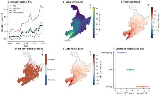
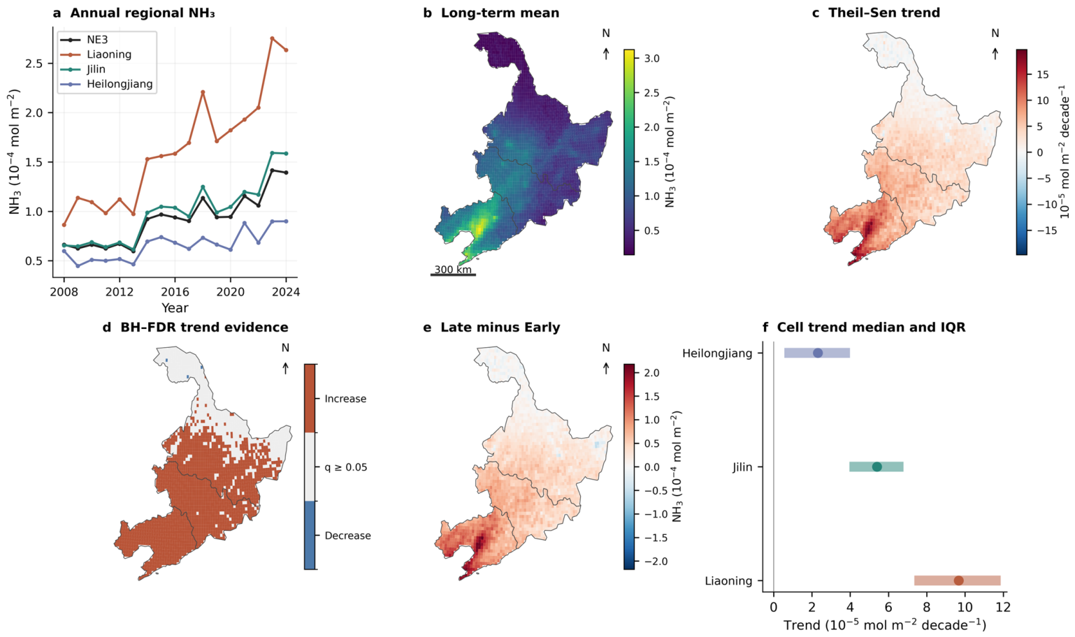
Atmospheric NH₃ increased widely during 2008–2024, with larger changes toward southern NE3. The regional Theil–Sen slope was 4.52 × 10⁻⁵ mol m⁻² decade⁻¹ (95% confidence interval, 3.12–5.70 × 10⁻⁵). The annual mean rose from 0.66 × 10⁻⁴ mol m⁻² in 2008 to 1.39 × 10⁻⁴ in 2024, following a maximum of 1.42 × 10⁻⁴ in 2023. Considerable interannual fluctuations accompanied recurring warm-season peaks. Provincial slopes were 9.83, 5.58 and 2.16 × 10⁻⁵ mol m⁻² decade⁻¹ in Liaoning, Jilin and Heilongjiang, respectively; their area-weighted median cell slopes were 9.67, 5.40 and 2.31. Provincial endpoint means increased from 0.86 to 2.63, 0.65 to 1.59 and 0.60 to 0.90 × 10⁻⁴ mol m⁻². The agreement between regional series and cell distributions shows a broad geographical gradient. Positive regional and provincial trends persisted in both HAC sensitivities (Figure 2a,c,f; Table S3).

Figure 2. NH₃ evolution in NE3, 2008–2024. (a) Area-weighted annual regional and provincial means; (b) mean monthly column; (c) cell Theil–Sen decadal trend; (d) increasing/decreasing trends passing BH–FDR q < 0.05, with other cells grey; (e) Late (2019–2024) minus Early (2008–2012) mean annual column; (f) area-weighted median and interquartile range of cell slopes. Finite negative retrievals are retained. Maps use clipped 0.2° cells in WGS84 Lambert conformal conic projection (40° N/52° N, 126° E); white is outside the represented domain. Columns and differences are in 10⁻⁴ mol m⁻²; slopes are in 10⁻⁵ mol m⁻² decade⁻¹.

Positive cell slopes covered 93.6% of represented NE3 area, and 71.2% met the ordinary Mann–Kendall/BH–FDR increasing-trend criterion. The latter fractions were 100.0% in Liaoning, 96.8% in Jilin and 50.7% in Heilongjiang. Despite northward differences in individual-cell significance, temporal block bootstrap confirmed positive trends for NE3 and all three provinces (NE3 95% CI: 3.34–5.50 × 10⁻⁵ mol m⁻² decade⁻¹). Field significance further showed that the observed 93.6% positive-trend area exceeded the null 95th percentile of 75.4% (p < 0.001; Table S6). Larger trends broadly overlapped the southern and southwestern high-column background. Mean cell increases between Early and Late were 1.11 × 10⁻⁴ mol m⁻² in Liaoning, 0.60 × 10⁻⁴ in Jilin and 0.26 × 10⁻⁴ in Heilongjiang, reinforcing the existing geographical contrast (Figure 2b–e; Table S3).

The main descriptive findings were insensitive to overpass selection and support filtering. AM produced a regional decadal trend of 4.79 × 10⁻⁵ mol m⁻² and seasonal amplification of 119.8%, compared with 4.52 × 10⁻⁵ and 119.7% for AM+PM; both retained the provincial trend hierarchy. Applying fractional support ≥0.25 to AM+PM gave 4.53 × 10⁻⁵ and 119.5%. Only 0.361% of its support records fell below this threshold, predominantly in winter (Figure S3; Table S1). Negative-response and incomplete-record exclusions for model fitting were concentrated in lower-column conditions, so the model-valid observations differ in support from the complete descriptive record (Figure S4; Table S4).

3.2. Strengthening Seasonality and Spatial Reorganization

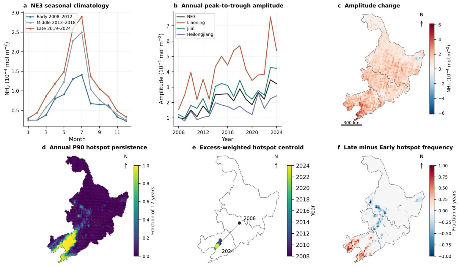
The increase in mean abundance was accompanied by a stronger annual cycle. Regional climatological peak-to-trough amplitude rose from 1.18 × 10⁻⁴ mol m⁻² in Early to 2.59 × 10⁻⁴ in Late, a 119.7% increase calculated before rounding. The Middle climatology already showed a larger warm-season peak, while winter columns changed less. Provincial amplitudes increased from 2.73 to 4.47 × 10⁻⁴ mol m⁻² in Liaoning, 1.57 to 2.90 in Jilin and 0.86 to 1.84 in Heilongjiang, corresponding to 63.6%, 85.1% and 113.9%. Liaoning retained the largest absolute cycle, whereas Heilongjiang amplified most relative to its smaller initial amplitude. Annual amplitudes fluctuated, but the regional JJA–DJF contrast and first-harmonic amplitude also increased, by 118.0% and 108.0%. Positive Late-minus-Early amplitude differences covered 96.7% of represented area, with larger absolute changes toward the south and southwest (Figure 3a–c and Figure S6; Table S7). The 2013–2014 rise persisted in Metop-A alone (103.7 versus 121.8 μmol m⁻² in merged data on matched support). Change-point tests found no clearly supported 2014/2020 step, and overlap-offset sensitivity retained a decadal trend of 4.63 × 10⁻⁵ mol m⁻² and 118.8% seasonal amplification (Table S8).

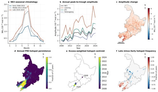
Figure 3. Seasonal amplification and hotspot reorganization, 2008–2024. (a) Early (2008–2012), Middle (2013–2018) and Late (2019–2024) regional monthly climatologies; (b) annual regional peak-to-trough amplitude; (c) Late-minus-Early cell climatological amplitude; (d) annual P90 hotspot persistence across seventeen years; (e) annual centroids weighted by overlap area and positive excess above annual area-weighted P90; (f) Late-minus-Early hotspot frequency. Centroid colour identifies year, and displacement uses WGS84 geodesics. Projection follows Figure 2. Climatologies and amplitudes are in 10⁻⁴ mol m⁻²; persistence and frequency differences are dimensionless.

A persistent high-column core remained in Liaoning. Cells exceeding the annual area-weighted P90 in at least fourteen of seventeen years occupied 6.4% of NE3 area and 34.1% of Liaoning’s represented area; provincial fractions rounded to 0.0% in Jilin and Heilongjiang. Liaoning’s mean annual fraction above P90 increased from 38.2% in Early to 50.3% in Late. Hotspot frequency rose in the southern core and declined in several northerly locations, indicating redistribution of the annual upper tail. The P80/P95 sensitivities preserved this southern emphasis, and fixed-P90 exceedance supplied a complementary comparison against a common absolute threshold (Figure 3d,f and Figure S7; Table S9).

The relative-P90 hotspot centroid showed robust southwestward trends during 2008–2024, with Theil–Sen slopes of −4.77 km yr⁻¹ eastward (95% block-bootstrap CI: −6.71 to −2.53) and −5.68 km yr⁻¹ northward (−7.98 to −3.00). Both directions persisted after excluding 2008 (−4.26 and −4.56 km yr⁻¹, respectively). Endpoint displacement varied substantially with the starting year (477.4 km for 2008–2024 versus 46.8 km for 2009–2024). The consistent coordinate trends, also supported by relative-P80 and P95 thresholds, indicate southwestward reorganization around a persistent southern hotspot core despite interannual fluctuations (Figure 3e and Figure S7; Tables S9 and S10).

3.3. Nonlinear Environmental Associations Identified by Ust-Bart

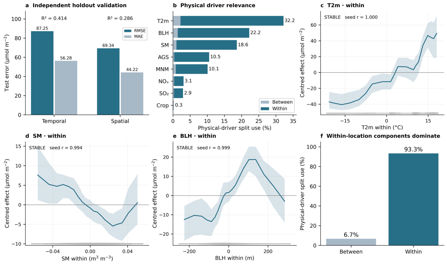
UST-BART supplied predictive information across both prescribed holdouts (Table 2A). Temporal testing gave RMSE 87.25 μmol m⁻², MAE 56.28 and R² 0.414; eastern spatial testing gave 69.34, 44.22 and 0.286. Mean biases were +2.09 and +0.96 μmol m⁻². Background-only XBART had temporal and spatial R² of 0.075 and −0.020, with larger errors in both tests. Physical predictors therefore added information beyond geographical and calendar backgrounds, although location-mean residual Moran’s I remained high at 0.717 and 0.493 (Figure 4a and Figure S14; Table S16). Compared with undecomposed XBART, UST-BART achieved higher spatial holdout R² (0.286 versus 0.206) and lower RMSE (69.34 versus 73.13 μmol m⁻²), whereas the undecomposed model performed better in temporal validation (R²: 0.492 versus 0.414; Table S17).

Table 2. (A) Holdout performance and background-only comparison. (B) Principal conditional-response summaries.

(A)
Model	Holdout	RMSE	MAE	R2	Mean Bias	Moran’s I
UST-BART	Temporal	87.25	56.28	0.414	2.09	0.717
Background-only XBART	Temporal	109.56	71.86	0.075	−21.85	—
UST-BART	Spatial	69.34	44.22	0.286	0.961	0.493
Background-only XBART	Spatial	82.87	54.38	−0.020	−1.22	—
(B)
Analysis	Metric		Estimate	Lower 95%	Upper 95%	Unit
Temperature within	Seed shape r		1.000	—	—	1
SM within	Seed shape r		0.994	—	—	1
BLH within	Seed shape r		0.999	—	—	1
Temperature within	P5–P95 net change		84.49	—	—	μmol m−2
Temperature × BLH	Mixed-contrast RMS		25.02	—	—	μmol m−2
Temperature × BLH	Seed surface r		0.978	—	—	1
Temperature × BLH	Peak local mixed contrast		64.41	22.99	96.73	μmol m−2
Temperature × SM	Mixed-contrast RMS		15.75	—	—	μmol m−2
Temperature × SM	Seed surface r		0.931	—	—	1
Temperature × SM	Peak local mixed contrast		−41.94	−78.30	−6.13	μmol m−2

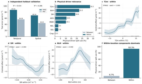
Figure 4. UST-BART validation and environmental responses, 2008–2022. (a) Temporal and eastern spatial holdout RMSE/MAE, with R² annotated; (b) split-use relevance normalized over physical components and divided into between/within shares; (c–e) within-location temperature, soil-moisture and BLH ALE over P5–P95; (f) between/within physical split shares. Background splits are excluded, and cropland has only a between component. Departures from overall location means contain seasonality. Blue curves are forest medians, light-blue shading indicates approximate 95% forest-response bands, horizontal grey lines mark zero effect, and bottom grey strips show predictor data density; seed shape agreement is annotated. Response units are μmol m⁻²; predictor units are °C, m³ m⁻³ and m.

On identical nonnegative test observations, the primary UST-BART model had mean biases of +49.32 and +51.76 μmol m⁻² in the lowest observed NH₃ decile for temporal (n = 9638; ≤17.86 μmol m⁻²) and spatial (n = 7080; ≤13.74 μmol m⁻²) validation, respectively. The auxiliary model retaining finite signed retrievals yielded lower low-decile biases of +35.21 and +36.38 μmol m⁻², with RMSE decreasing from 59.58 to 51.61 and from 58.11 to 47.25 μmol m⁻², respectively. On the full matched nonnegative test sets, however, the primary model retained slightly higher R² (0.414 vs. 0.406 temporally; 0.286 vs. 0.252 spatially; Table S18).

Meteorology dominated physical-driver split use: temperature accounted for 32.2%, BLH 22.2% and soil moisture 18.6%. AGS and MNM contributed 10.5% and 10.1%, followed by NO_x (3.1%), SO₂ (2.9%) and cropland (0.3%). Within-location components comprised 93.3% and between components 6.7% of physical splits. Within-temperature had the clearest positive ALE response, with a mean P5–P95 endpoint contrast of +84.5 μmol m⁻² and seed shape correlation rounding to 1.000. Its curve had flatter sections and a steeper warm end, moving from negative centred effects below the location mean to positive effects above it (Figure 4b,c,f; Tables S12 and S13).

Within-soil moisture showed a reproducible U-shaped association (seed r = 0.994): effects declined from drier departures to a lower region at moderately positive departures, then increased toward wetter conditions. Within-BLH was broadly inverse-U (r = 0.999), rising from strongly negative departures before declining at larger positive departures. The changing slopes make a single signed coefficient inadequate. First-half versus second-half forest means reproduced these core meteorological shapes with correlations above 0.98, although band endpoints varied more than means (Figure 4d,e and Figure S10; Table S19).

Between-temperature had a smaller positive endpoint contrast of +8.5 μmol m⁻² (seed r = 0.978); other between curves were generally weaker or less reproducible, including unstable between-soil moisture. Annual AGS departures showed declining effects toward central values followed by flatter portions, while several secondary inventory curves changed mainly near the centre of their ranges. These annual relationships differ in temporal support from the monthly meteorological curves. Collinear inventories, cropland and geographical terms can also share predictive information, so split ranking alone does not establish the importance of agriculture or chemistry (Figures S9 and S10d–g; Tables S12 and S13). The principal conditional-response estimates are summarized in Table 2B.

Temporal training/testing: 2008–2018/2019–2022 (96,379 test rows). Spatial testing: longitude ≥ 129.5° E (70,797 rows, 470 locations). Errors and predicted-minus-observed bias use μmol m⁻² and equal row weights. Moran’s I uses four nearest neighbours of location-mean residuals.

Estimates are forest means except seed correlations. Approximate 95% GFR response bands are pointwise and exclude observation noise. Response units are μmol m⁻²; r is dimensionless. Temperature net change spans P5–P95.

3.4. Non-Additive Responses, Province Heterogeneity and Observed Evolution

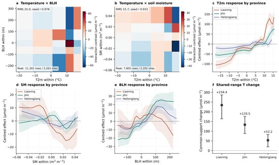
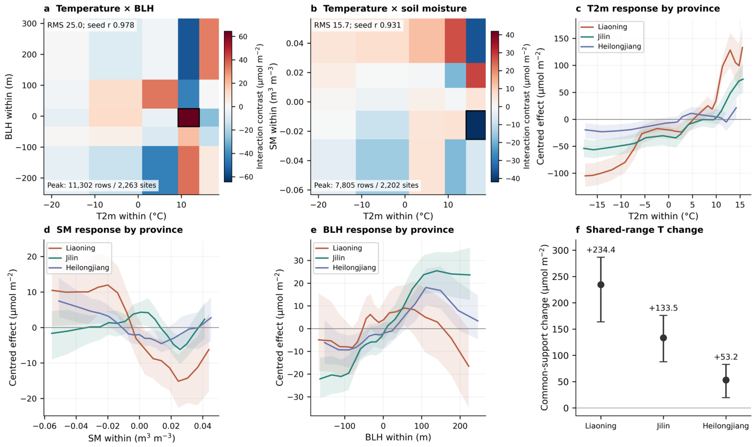
The leading temperature × BLH within-location interaction had mixed-contrast RMS 25.0 μmol m⁻² and seed surface correlation 0.978. Its peak supported local contrast was +64.4 μmol m⁻² (approximate band, +23.0 to +96.7): within that warm-departure rectangle, the temperature contrast was larger at the higher BLH endpoint. The temperature × soil-moisture interaction had RMS 15.7 μmol m⁻² and seed correlation 0.931. Its largest-magnitude contrast was −41.9 μmol m⁻² (−78.3 to −6.1), indicating a weaker temperature contrast at the higher moisture endpoint in the reported warm rectangle. Signs changed elsewhere on both surfaces, demonstrating dependence on joint conditions. All twenty-five rectangles were supported for each principal pair. Less reproducible agricultural-background combinations remained supplementary evidence (Figure 5a,b, Figures S11 and S12; Table 2B and Table S9).

Figure 5. Temperature interactions and provincial heterogeneity, 2008–2022. (a,b) Temperature within × BLH within and temperature within × soil moisture within local mixed contrasts (forest means, μmol m⁻²). Red and blue colors indicate positive and negative local mixed contrasts, respectively. Rectangles require ≥50 rows and ≥10 locations; black outlines identify reported peak rectangles and their row/site support. Predictor units are °C, m and m³ m⁻³. (c–e) Province-specific within-location temperature, soil-moisture and BLH ALE from the same model, restricted to the intersection of provincial P5–P95 ranges; colored lines are forest medians, shaded areas indicate approximate 95% response bands, and horizontal grey lines indicate zero effect. (f) Forest-mean temperature endpoint changes across shared support, with response bands (μmol m⁻²). Curves are independently centred. Mixed contrasts are local four-corner differences; their bands are pointwise.

Provincial responses differed within the same UST-BART function. Across the shared temperature-departure interval of −18.42 to +15.85 °C, mean net responses were +234.4 μmol m⁻² in Liaoning (approximate band, +163.8 to +286.7), +133.5 in Jilin (+87.8 to +176.0) and +53.2 in Heilongjiang (+19.6 to +82.9). Paired same-forest contrasts retained that ordering (Tables S15 and S19). These values span the whole common interval. Independently centred curves compare contextual response shapes without measuring absolute provincial column offsets. Moisture curves differed in the depth and position of lower-effect regions; Liaoning’s BLH curve rose then declined, whereas Jilin retained a broader elevated upper portion. Annual AGS departures showed a more pronounced decline toward central values in Liaoning and smaller changes elsewhere (Figure 5c–f and Figure S13).

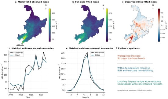
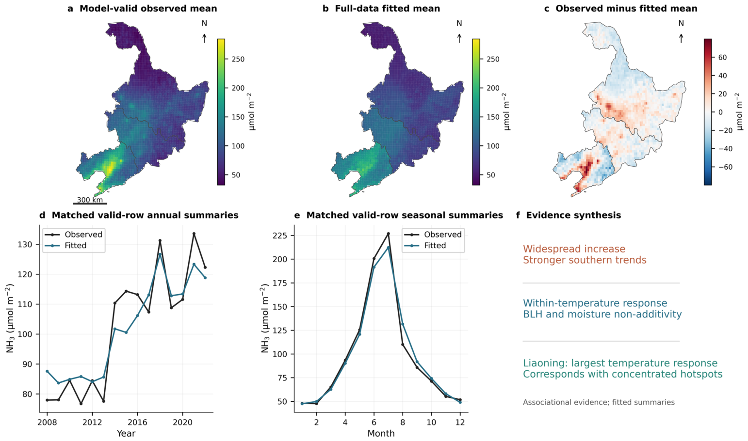
Liaoning thus combined the strongest common-range temperature response with the largest long-term trend, strongest absolute seasonal cycle and persistent hotspot core. On identical valid-model rows, full-data fitted spatial, annual and monthly summaries reproduced broad southern concentration and seasonal structure (Figure 6). This descriptive correspondence links environmental responses to the observed pattern, while the held-out tests provide the independent predictive evidence. The selected 2008–2022 record and its full-data fit cannot establish the causes of the longer 2008–2024 increase.

Figure 6. Observed and full-data fitted NH₃ on identical valid-model support, 2008–2022. (a,b) Observed and two-seed forest-mean fitted location means; (c) observed minus fitted; (d,e) area-weighted annual/monthly summaries of the same 354,539 rows; (f) correspondence between descriptive patterns and conditional responses. Units are μmol m⁻². The selected observed series differs from the complete record in Figure 2. Full-data fitted summaries are descriptive, and panel (f) does not indicate causation.

4. Discussion

4.1. Seasonal Amplification and the Persistent Southern Core

Increasing NH₃ abundance in NE3 involved a stronger annual cycle and reinforcement of the southern high-column core. The direction agrees with earlier IASI evidence of increasing East Asian columns during 2008–2018 [14]. Extending the record to 2024 and resolving the three provinces reveals how annual abundance, seasonal amplitude and recurring high-column locations evolved together. Seasonal amplitude more than doubled, with summer–winter and harmonic measures pointing to disproportionate warm-season enhancement. Instrument-overlap evidence supports this pattern, while IASI retrieval sensitivity to thermal contrast may affect winter minima [13] (Table S8). Historical inventories show pronounced spring and summer peaks in Chinese NH₃ emissions [6]. That source-seasonality context is relevant, but the changing atmospheric cycle also incorporates weather, transport and chemical processing. Liaoning’s large absolute cycle and Heilongjiang’s greater proportional amplification identify different aspects of the regional monitoring problem.

The persistent Liaoning core gives this seasonal change a clear geographical focus. A recent national assessment also found increasing NH₃ concentrations over its Northeast China Plain subregion using CrIS, ground observations and modelling [27]. Its variable and regional definition differ from the present total-column analysis, which identifies recurrent upper-tail locations within administrative NE3. Annual P90 is a relative threshold: increasing Liaoning hotspot frequency indicates redistribution of high ranks across the domain, while the fixed-threshold sensitivity describes absolute exceedance. The unusually northerly 2008 centroid magnified the endpoint displacement, whereas the robust relative-P90 coordinate trends indicate southwestward reorganization around a persistent southern core amid year-to-year fluctuations.

4.2. Joint Meteorological Responses and Atmospheric Processing

The nonlinear responses show why monthly variability cannot be summarized by one environmental coefficient. The positive temperature association, particularly at its warm end, is physically plausible given temperature- and moisture-dependent NH₃ exchange between land and atmosphere [46]. It also corresponds with stronger warm-season columns. Since departures are calculated from each location’s overall mean, however, the response includes seasonality and does not isolate climatic warming. Moisture adds a different pattern: both drier and wetter departures can accompany higher fitted columns. Experiments on urea-treated soil show that initial moisture and the timing and amount of wetting jointly affect hydrolysis and volatilization [47]. These processes motivate joint interpretation but cannot identify which mechanism produced either branch of the regional U-shaped curve. The local temperature–moisture contrasts further show that one response changes with the state of the other.

BLH likewise modifies the temperature contrast, with the leading warm-departure rectangle showing a larger contrast at its higher BLH endpoint. Opposite signs elsewhere and the broadly inverse-U first-order curve indicate dependence on context. Vertical redistribution alone does not reduce a total column in the way it can dilute a near-surface concentration. Regional atmospheric transport can nevertheless redistribute NH₃ between source and receptor regions, contributing to differences in observed columns. Chemical transport modelling has also demonstrated the importance of meteorological variability for atmospheric NH₃ [21,24]. Emissions, transport, atmospheric partitioning and retrieval sensitivity may all accompany BLH changes; the fitted surface summarizes their combined conditional association. Its supported local contrasts identify environmental combinations worth testing with collocated measurements, without resolving those pathways individually.

The dominance of meteorological split use also reflects the information available to the model. Weather varies monthly, whereas inventories repeat annual agricultural emissions across all twelve months and cannot resolve fertilizer or manure timing. Lower inventory relevance therefore does not diminish the importance of agricultural sources. Nor do small SO₂ and NO_x shares exclude chemical control: North China Plain observations and simulations linked reduced sulfate formation to increasing gas-phase NH₃ despite declining estimated NH₃ emissions [20]. Chemical transport simulations for eastern China further demonstrated that changes in SO₂ and NO_x emissions can influence gas–particle partitioning through the sulfate–nitrate–ammonium system [21]. Together with meteorological influences on surface exchange and atmospheric transport [24,26], these processes provide a physical context for the observed seasonal amplification of atmospheric NH₃. The 119.7% increase quantified in this study therefore represents the amplification of atmospheric NH₃ column seasonality rather than a corresponding increase in NH₃ emissions.

4.3. Model Construction and Provincial Response Heterogeneity

UST-BART brings persistent location conditions, temporal departures and geographical/calendar context into one nonlinear response. The between/within distinction follows established longitudinal modelling practice [29]. Here it distinguishes a generally warmer location from a month that is warmer than that location’s own mean, while permitting both components to interact with other drivers. Estimation uses the existing accelerated BART procedure [31]. Applied to atmospheric NH₃, this structure provides distinct between- and within-location ALE responses, identifies supported interactions involving temperature, soil moisture and BLH, and enables province-specific comparisons within a shared nonlinear model. Common-support provincial comparisons reveal greater temperature responsiveness in Liaoning alongside its stronger observed seasonal cycle and trend. These common-support comparisons reveal province-specific environmental associations that complement the observed geographical differences in NH₃ trends and seasonality.

Independent temporal (2019–2022) and contiguous spatial (eastern Jilin and Heilongjiang) holdouts directly evaluate predictive transfer to later years and geographically withheld locations [33]. Compared with the background-only XBART model, UST-BART increased temporal R² from 0.075 to 0.414 and spatial R² from −0.020 to 0.286, while reducing RMSE from 109.56 to 87.25 and from 82.87 to 69.34 μmol m⁻², respectively. These results demonstrate that the environmental predictors provide meaningful predictive information across both independent holdouts. Although the RMSE values are numerically comparable to regional annual means (approximately 80–130 μmol m⁻²), they represent individual cell-month prediction errors rather than aggregated annual columns. Residual Moran’s I values of 0.717 and 0.493 indicate remaining spatially structured variation, highlighting opportunities to improve local-scale predictions. The reported temperature response of +84.5 μmol m⁻² represents the fitted ALE endpoint contrast across the P5–P95 range of within-location temperature departures, rather than a per-degree temperature coefficient. The ALE curves and provincial comparisons characterize observation-supported conditional environmental associations represented by the fitted function, providing insights into the nonlinear environmental dependence of atmospheric NH₃. An additional comparison with undecomposed predictors yielded higher temporal R² for the undecomposed model (0.492 versus 0.414), whereas UST-BART achieved higher spatial R² (0.286 versus 0.206). The between/within specification thus provides a clearer distinction between persistent spatial conditions and within-location environmental variation, together with stronger performance in the tested spatial holdout. The principal nonlinear response patterns were consistently reproduced across random seeds and retained-sample halves, further supporting the stability of the fitted environmental associations.

4.4. Regional Implications and Interpretation Boundaries

For example, warm-season NH₃ monitoring could prioritize Liaoning’s persistent hotspot core, alongside repeated observations at representative Heilongjiang sites to capture the stronger proportional seasonal amplification farther north. Crop-specific fertilizer and manure records would help distinguish source timing from atmospheric conditions; improving fertilizer calendars and crop allocation has already improved Chinese inventory agreement with observations [7]. The response surfaces can guide sampling across contrasting moisture and boundary layer states. They do not prescribe optimal management schedules. Agricultural NH₃ mitigation has potentially large societal benefits [5]. Its atmospheric consequences nevertheless depend on co-pollutants: Chinese modelling found reductions in particulate pollution and deposition alongside increased precipitation acidification under some NH₃-control scenarios [4]. The present maps identify priority conditions and locations for such assessments, without estimating PM₂.₅, deposition, health or economic outcomes.

The descriptive analyses retain finite signed IASI retrievals through 2024, whereas the primary UST-BART model uses nonnegative complete observations through 2022, consistent with EDGAR availability. An auxiliary fit retaining signed retrievals showed lower low-column predictive bias on matched tests, but did not improve overall holdout R² (Table S18); the primary response curves therefore describe the selected modelling sample. The four-year temporal test (2019–2022) provides an out-of-time evaluation, while the full modelling period spans the Metop-A/B and Metop-B/C transitions; their observational implications are examined in the instrument-overlap sensitivity analysis. Annual inventories and static 2020 cropland cannot represent monthly source timing or land-cover change. IASI reanalysis also uses ERA5 atmospheric inputs, introducing potential dependence between meteorological predictors and retrieval sensitivity [13]. Finally, the approximate GFR response bands omit observation noise and retrieval-error propagation, and the interaction bands are pointwise. These limitations do not alter the documented regional patterns, but they constrain their explanation. Seasonal source records, collocated atmospheric profiles and chemical transport analysis would help distinguish emissions, processing and retrieval contributions to the observed change.

5. Conclusions

NH₃ columns increased across Northeast China during 2008–2024 at a regional rate of 4.52 × 10⁻⁵ mol m⁻² decade⁻¹, accompanied by a 119.7% increase in the seasonal peak-to-trough amplitude of atmospheric NH₃ columns and a persistent Liaoning hotspot core. This amplitude change does not represent an NH₃ emission increase. Relative-P90 centroid endpoint displacement was start-year-sensitive (477.4 versus 46.8 km), while Theil–Sen trends supported southwestward hotspot reorganization. Liaoning retained the greatest absolute seasonal amplitude, whereas Heilongjiang showed the greatest proportional provincial increase. The constructed UST-BART model joined location means and temporal departures with spatial and calendar context, identifying a positive temperature response, U-shaped soil-moisture response and broadly inverse-U BLH response. Local interactions and common-support provincial curves showed that temperature associations varied with accompanying conditions and were strongest in Liaoning. Temporal and spatial holdouts confirmed added predictive information from physical drivers, although incomplete skill and remaining spatial residual structure limit inference. The findings support geographically focused warm-season monitoring and closer observation of seasonal growth in the north. They establish changes in atmospheric columns and context-dependent associations; causal attribution requires independent source and atmospheric-process evidence.

References

- Huang, X.; Song, Y.; Li, M.; Li, J.; Huo, Q.; Cai, X.; Zhu, T.; Hu, M.; Zhang, H. A high-resolution ammonia emission inventory in China. Glob. Biogeochem. Cycles 2012, 26, GB1030. [Google Scholar] [CrossRef] [Scilit]
- Liu, X.; Zhang, Y.; Han, W.; Tang, A.; Shen, J.; Cui, Z.; Vitousek, P.; Erisman, J.W.; Goulding, K.; Christie, P.; et al. Enhanced nitrogen deposition over China. Nature 2013, 494, 459–462. [Google Scholar] [CrossRef] [Scilit] [PubMed]
- Wang, Y.; Zhang, Q.Q.; He, K.; Zhang, Q.; Chai, L. Sulfate-nitrate-ammonium aerosols over China: Response to 2000–2015 emission changes of sulfur dioxide, nitrogen oxides, and ammonia. Atmos. Chem. Phys. 2013, 13, 2635–2652. [Google Scholar] [CrossRef] [Scilit]
- Liu, M.; Huang, X.; Song, Y.; Tang, J.; Cao, J.; Zhang, X.; Zhang, Q.; Wang, S.; Xu, T.; Kang, L.; et al. Ammonia emission control in China would mitigate haze pollution and nitrogen deposition, but worsen acid rain. Proc. Natl. Acad. Sci. USA 2019, 116, 7760–7765. [Google Scholar] [CrossRef] [Scilit] [PubMed]
- Zhang, X.; Gu, B.; van Grinsven, H.; Lam, S.K.; Liang, X.; Bai, M.; Chen, D. Societal benefits of halving agricultural ammonia emissions in China far exceed the abatement costs. Nat. Commun. 2020, 11, 4357. [Google Scholar] [CrossRef] [Scilit] [PubMed]
- Kang, Y.; Liu, M.; Song, Y.; Huang, X.; Yao, H.; Cai, X.; Zhang, H.; Kang, L.; Liu, X.; Yan, X.; et al. High-resolution ammonia emissions inventories in China from 1980 to 2012. Atmos. Chem. Phys. 2016, 16, 2043–2058. [Google Scholar] [CrossRef] [Scilit]
- Li, B.; Chen, L.; Shen, W.; Jin, J.; Wang, T.; Wang, P.; Yang, Y.; Liao, H. Improved gridded ammonia emission inventory in China. Atmos. Chem. Phys. 2021, 21, 15883–15900. [Google Scholar] [CrossRef] [Scilit]
- Zhan, X.; Adalibieke, W.; Cui, X.; Winiwarter, W.; Reis, S.; Zhang, L.; Bai, Z.; Wang, Q.; Huang, W.; Zhou, F. Improved Estimates of Ammonia Emissions from Global Croplands. Environ. Sci. Technol. 2021, 55, 1329–1338. [Google Scholar] [CrossRef] [Scilit] [PubMed]
- Clarisse, L.; Clerbaux, C.; Dentener, F.; Hurtmans, D.; Coheur, P.-F. Global ammonia distribution derived from infrared satellite observations. Nat. Geosci. 2009, 2, 479–483. [Google Scholar] [CrossRef] [Scilit]
- Van Damme, M.; Clarisse, L.; Heald, C.L.; Hurtmans, D.; Ngadi, Y.; Clerbaux, C.; Dolman, A.J.; Erisman, J.W.; Coheur, P.F. Global distributions, time series and error characterization of atmospheric ammonia (NH3) from IASI satellite observations. Atmos. Chem. Phys. 2014, 14, 2905–2922. [Google Scholar] [CrossRef] [Scilit]
- Whitburn, S.; Van Damme, M.; Clarisse, L.; Bauduin, S.; Heald, C.L.; Hadji-Lazaro, J.; Hurtmans, D.; Zondlo, M.A.; Clerbaux, C.; Coheur, P.-F. A flexible and robust neural network IASI-NH3 retrieval algorithm. J. Geophys. Res. Atmos. 2016, 121, 6581–6599. [Google Scholar] [CrossRef] [Scilit]
- Van Damme, M.; Whitburn, S.; Clarisse, L.; Clerbaux, C.; Hurtmans, D.; Coheur, P.-F. Version 2 of the IASI NH3 neural network retrieval algorithm: Near-real-time and reanalysed datasets. Atmos. Meas. Tech. 2017, 10, 4905–4914. [Google Scholar] [CrossRef] [Scilit]
- Clarisse, L.; Franco, B.; Van Damme, M.; Di Gioacchino, T.; Hadji-Lazaro, J.; Whitburn, S.; Noppen, L.; Hurtmans, D.; Clerbaux, C.; Coheur, P. The IASI NH3 version 4 product: Averaging kernels and improved consistency. Atmos. Meas. Tech. 2023, 16, 5009–5028. [Google Scholar] [CrossRef] [Scilit]
- Van Damme, M.; Clarisse, L.; Franco, B.; Sutton, M.A.; Erisman, J.W.; Wichink Kruit, R.; van Zanten, M.; Whitburn, S.; Hadji-Lazaro, J.; Hurtmans, D.; et al. Global, regional and national trends of atmospheric ammonia derived from a decadal (2008–2018) satellite record. Environ. Res. Lett. 2021, 16, 055017. [Google Scholar] [CrossRef] [Scilit]
- Warner, J.X.; Dickerson, R.R.; Wei, Z.; Strow, L.L.; Wang, Y.; Liang, Q. Increased atmospheric ammonia over the world’s major agricultural areas detected from space. Geophys. Res. Lett. 2017, 44, 2875–2884. [Google Scholar] [CrossRef] [Scilit] [PubMed]
- Van Damme, M.; Clarisse, L.; Whitburn, S.; Hadji-Lazaro, J.; Hurtmans, D.; Clerbaux, C.; Coheur, P.-F. Industrial and agricultural ammonia point sources exposed. Nature 2018, 564, 99–103. [Google Scholar] [CrossRef] [Scilit] [PubMed]
- Dammers, E.; McLinden, C.A.; Griffin, D.; Shephard, M.W.; Van Der Graaf, S.; Lutsch, E.; Schaap, M.; Gainairu-Matz, Y.; Fioletov, V.; Van Damme, M.; et al. NH3 emissions from large point sources derived from CrIS and IASI satellite observations. Atmos. Chem. Phys. 2019, 19, 12261–12293. [Google Scholar] [CrossRef] [Scilit]
- Guo, X.; Wang, R.; Pan, D.; Zondlo, M.A.; Clarisse, L.; Van Damme, M.; Whitburn, S.; Coheur, P.-F.; Clerbaux, C.; Franco, B.; et al. Validation of IASI satellite ammonia observations at the pixel scale using in situ vertical profiles. J. Geophys. Res. Atmos. 2021, 126, e2020JD033475. [Google Scholar] [CrossRef] [Scilit]
- Zheng, B.; Tong, D.; Li, M.; Liu, F.; Hong, C.; Geng, G.; Li, H.; Li, X.; Peng, L.; Qi, J.; et al. Trends in China’s anthropogenic emissions since 2010 as the consequence of clean air actions. Atmos. Chem. Phys. 2018, 18, 14095–14111. [Google Scholar] [CrossRef] [Scilit]
- Liu, M.; Huang, X.; Song, Y.; Xu, T.; Wang, S.; Wu, Z.; Hu, M.; Zhang, L.; Zhang, Q.; Pan, Y.; et al. Rapid SO2 emission reductions significantly increase tropospheric ammonia concentrations over the North China Plain. Atmos. Chem. Phys. 2018, 18, 17933–17943. [Google Scholar] [CrossRef] [Scilit]
- Lachatre, M.; Fortems-Cheiney, A.; Foret, G.; Siour, G.; Dufour, G.; Clarisse, L.; Clerbaux, C.; Coheur, P.-F.; Van Damme, M.; Beekmann, M. The unintended consequence of SO2 and NO2 regulations over China: Increase of ammonia levels and impact on PM2.5 concentrations. Atmos. Chem. Phys. 2019, 19, 6701–6716. [Google Scholar] [CrossRef] [Scilit]
- Luo, Z.; Zhang, Y.; Chen, W.; Van Damme, M.; Coheur, P.-F.; Clarisse, L. Estimating global ammonia (NH3) emissions based on IASI observations from 2008 to 2018. Atmos. Chem. Phys. 2022, 22, 10375–10388. [Google Scholar] [CrossRef] [Scilit]
- Evangeliou, N.; Balkanski, Y.; Eckhardt, S.; Cozic, A.; Van Damme, M.; Coheur, P.-F.; Clarisse, L.; Shephard, M.W.; Cady-Pereira, K.E.; Hauglustaine, D. 10-year satellite-constrained fluxes of ammonia improve performance of chemistry transport models. Atmos. Chem. Phys. 2021, 21, 4431–4451. [Google Scholar] [CrossRef] [Scilit]
- Schiferl, L.D.; Heald, C.L.; Van Damme, M.; Clarisse, L.; Clerbaux, C.; Coheur, P.-F.; Nowak, J.B.; Neuman, J.A.; Herndon, S.C.; Roscioli, J.R.; et al. Interannual variability of ammonia concentrations over the United States: Sources and implications. Atmos. Chem. Phys. 2016, 16, 12305–12328. [Google Scholar] [CrossRef] [Scilit]
- Lan, Z.; Zhang, X.; Lin, W.; Xu, X.; Ma, Z.; Jin, J.; Wu, L.; Zhang, Y. Atmospheric NH3 in urban Beijing: Long-term variations and implications for secondary inorganic aerosol control. Atmos. Chem. Phys. 2024, 24, 9355–9368. [Google Scholar] [CrossRef] [Scilit]
- Liu, L.; Zhang, X.; Xu, W.; Liu, X.; Li, Y.; Lu, X.; Zhang, Y.; Zhang, W. Temporal characteristics of atmospheric ammonia and nitrogen dioxide over China based on emission data, satellite observations and atmospheric transport modeling since 1980. Atmos. Chem. Phys. 2017, 17, 9365–9378. [Google Scholar] [CrossRef] [Scilit]
- Sun, F.; Cui, Y.; Su, J.; Shephard, M.W.; Kharol, S.K.; Zhang, Y.; Shi, X.; Zhang, J.; Liu, H.; Xiao, Q.; et al. Decadal changes in atmospheric ammonia and dry deposition across China inferred from space-ground measurements and model simulations. Atmos. Chem. Phys. 2025, 25, 17907–17932. [Google Scholar] [CrossRef] [Scilit]
- Sheng, M.; Zhou, R.; Hua, J.; Han, S.; Liu, S.; Zhang, L.; Wang, W.; Dang, R.; Cao, H.; Chen, Z.; et al. Geostationary observations of atmospheric ammonia over East Asia: Spatio-temporal variations revealed by three years of FY-4B/GIIRS measurements. Atmos. Chem. Phys. 2026, 26, 7803–7826. [Google Scholar] [CrossRef] [Scilit]
- Curran, P.J.; Bauer, D.J. The disaggregation of within-person and between-person effects in longitudinal models of change. Annu. Rev. Psychol. 2011, 62, 583–619. [Google Scholar] [CrossRef] [Scilit] [PubMed]
- Chipman, H.A.; George, E.I.; McCulloch, R.E. BART: Bayesian additive regression trees. Ann. Appl. Stat. 2010, 4, 266–298. [Google Scholar] [CrossRef] [Scilit]
- He, J.; Yalov, S.; Hahn, P.R. XBART: Accelerated Bayesian Additive Regression Trees. In Proceedings of the Twenty-Second International Conference on Artificial Intelligence and Statistics. Proc. Mach. Learn. Res. 2019, 89, 1130–1138. Available online: https://proceedings.mlr.press/v89/he19a.html (accessed on 1 September 2026).
- Apley, D.W.; Zhu, J. Visualizing the effects of predictor variables in black box supervised learning models. J. R. Stat. Soc. Ser. B Stat. Methodol. 2020, 82, 1059–1086. [Google Scholar] [CrossRef] [Scilit]
- Roberts, D.R.; Bahn, V.; Ciuti, S.; Boyce, M.S.; Elith, J.; Guillera-Arroita, G.; Hauenstein, S.; Lahoz-Monfort, J.J.; Schröder, B.; Thuiller, W.; et al. Cross-validation strategies for data with temporal, spatial, hierarchical, or phylogenetic structure. Ecography 2017, 40, 913–929. [Google Scholar] [CrossRef] [Scilit]
- Clarisse, L.; Van Damme, M.; Coheur, P. ESA Precursors for Aerosols and Ozone Climate Change Initiative (Precursors_cci): IASI NH3 L3 Merged Product, Version 4R (4.0.1R). NERC EDS Centre for Environmental Data Analysis. 2026. Available online: https://catalogue.ceda.ac.uk/uuid/2ec5b1fb653445bdbbd0dcd69dd223da/ (accessed on 12 October 2026).
- ESA Climate Change Initiative. D4.2 Product User Guide, version 01_01. 2024. Available online: https://climate.esa.int/documents/2636/Precursors_cci_D4.2_PUG_01_01.pdf (accessed on 12 October 2026).
- ECMWF. ERA5 Monthly Averaged Data on Single Levels. Climate Data Store. Available online: https://cds.climate.copernicus.eu/datasets/reanalysis-era5-single-levels-monthly-means (accessed on 12 October 2026).
- ECMWF. ERA5-Land Monthly Averaged Data from 1950 to Present. Climate Data Store. Available online: https://cds.climate.copernicus.eu/datasets/reanalysis-era5-land-monthly-means (accessed on 12 October 2026).
- European Commission, Joint Research Centre. Global Air Pollutant Emissions. EDGAR v8.1. Available online: https://edgar.jrc.ec.europa.eu/dataset_ap81 (accessed on 12 October 2026).
- Sulla-Menashe, D.; Friedl, M.A. User Guide to Collection 6 MODIS Land Cover (MCD12Q1 and MCD12C1) Product, with the Collection 6.1 Supplement. LP DAAC. 2022. Available online: https://lpdaac.usgs.gov/documents/1409/MCD12_User_Guide_V61.pdf (accessed on 12 October 2026).
- geoBoundaries. gbOpen CHN ADM1, Boundary ID CHN-ADM1-43563684, Reference Year 2019. Pinned Repository Revision 9469f09. 2023. Available online: https://www.geoboundaries.org/api/current/gbOpen/CHN/ADM1/ (accessed on 12 October 2026).
- Sen, P.K. Estimates of the regression coefficient based on Kendall’s tau. J. Am. Stat. Assoc. 1968, 63, 1379–1389. [Google Scholar] [CrossRef]
- Newey, W.K.; West, K.D. A simple, positive semi-definite, heteroskedasticity and autocorrelation consistent covariance matrix. Econometrica 1987, 55, 703–708. [Google Scholar] [CrossRef] [Scilit]
- Mann, H.B. Nonparametric tests against trend. Econometrica 1945, 13, 245–259. [Google Scholar] [CrossRef] [Scilit]
- Benjamini, Y.; Hochberg, Y. Controlling the false discovery rate: A practical and powerful approach to multiple testing. J. R. Stat. Soc. Ser. B Methodol. 1995, 57, 289–300. [Google Scholar] [CrossRef] [Scilit]
- StochTree. Supervised Learning in StochTree. Installed Python Implementation Version 0.4.5. General Model and Sampler Documentation. 2026. Available online: https://stochtree.ai/about/bart.html (accessed on 12 October 2026).
- Sutton, M.A.; Reis, S.; Riddick, S.N.; Dragosits, U.; Nemitz, E.; Theobald, M.R.; Tang, Y.S.; Braban, C.F.; Vieno, M.; Dore, A.J.; et al. Towards a climate-dependent paradigm of ammonia emission and deposition. Philos. Trans. R. Soc. B Biol. Sci. 2013, 368, 20130166. [Google Scholar] [CrossRef] [Scilit] [PubMed]
- Black, A.S.; Sherlock, R.R.; Smith, N.P. Effect of timing of simulated rainfall on ammonia volatilization from urea, applied to soil of varying moisture content. J. Soil Sci. 1987, 38, 679–687. [Google Scholar] [CrossRef] [Scilit]
Disclaimer/Publisher’s Note: The statements, opinions and data contained in all publications are solely those of the individual author(s) and contributor(s) and not of MDPI and/or the editor(s). MDPI and/or the editor(s) disclaim responsibility for any injury to people or property resulting from any ideas, methods, instructions or products referred to in the content. |
© 2026 by the authors. Licensee MDPI, Basel, Switzerland. This article is an open access article distributed under the terms and conditions of the Creative Commons Attribution (CC BY) license.