National-Scale Climatological Assessment of Ground Snow Loads in Kazakhstan: Eurocode-Based Zoning from Five Decades of Observations

Abstract

Spatially differentiated snow-load assessment is essential for updating building provisions in Kazakhstan, where climatic contrasts and complex terrain produce substantial regional variations in snow accumulation. This study develops a national-scale methodology for ground snow load zoning consistent with the characteristic-value approach of Eurocode 1 (EN 1991-1-3:2003). The assessment uses observations from 210 Kazhydromet meteorological stations for 1971–2020 and snow survey data from 17 mountain river basins. Cluster analysis, minimum spanning tree regionalization, Gumbel extreme-value estimation, regional elevation-dependent regression relationships, and GIS mapping were combined to estimate characteristic ground snow loads with an annual exceedance probability of 0.02, corresponding to a 50-year mean return period. The resulting national map delineates nine snow-load zones, with assigned values of 0.8, 1.2, 1.5, 1.8, 2.4, 3.2, 4.0, 4.8 kPa and an open-ended highest class exceeding 5.6 kPa. Regional regression equations quantify elevation-related variations in snow loads within the investigated mountain and upland areas, complementing the geographical differentiation represented by the map. The results provide an observational and statistical basis for updating national snow-load provisions and selecting regionally appropriate ground snow loads for structural design. The underlying snow water equivalent data also support subsequent hydrological assessments of snow storage.

1. Introduction

The territory of Kazakhstan is characterized by exceptional spatiotemporal heterogeneity in snow cover formation and accumulation, with parameters varying from consistently high values across the northern, central, and eastern regions to pronounced instability in the southern part of the republic. Specifically, snowpack instability represents one of the most distinctive features of the winter landscape within the plains and foothills of southern Kazakhstan. The primary driver of this phenomenon is the winter thermal regime, which is characterized by frequent thaws, combined with a generally shallow snow depth. Furthermore, within the sandy and clay deserts of Kazakhstan, wind-blown snow mixes with soil particles, accelerating melt rates due to a significant reduction in surface albedo.

Climate change and repeated collapses of building roofs due to significant snow loads have made the standardisation of these loads and their consideration during the design of structures a highly topical issue [1,2,3].

An analysis of numerous studies has shown that the standardisation of snow loads in SNiP (Construction Norms and Rules) 2.01.07–85, issued by the State Committee of the USSR for Construction (Gosstroy USSR) [4], had a number of shortcomings in terms of microzoning, among which the most relevant should be highlighted:

• Insufficiently detailed territorial zoning;
• Kazakhstan’s vast territory is divided into just three zones: I—0.5 kPa, II—0.7 kPa, III—1.0 kPa;
• The inability to account for the service life of structures, leading to their design for an indefinite service life.

Consequently, Kazakhstan has sought to align its snow-load provisions with Eurocode 1 [3,5]. Under this framework, characteristic ground snow loads correspond to an annual exceedance probability of 0.02, or a mean return period of 50 years.

Globally, the assessment and standardization of snow loads rely on harmonized normative frameworks and advanced spatial analytical techniques. In Europe, extensive research within the European Snow Load Research Project (ESLRP) and Eurocode provisions (EN 1991-1-3, Annex C) has focused on unifying ground snow load maps across national borders to ensure structural consistency [5,6]. On an international level, standards such as ISO 4355 establish unified procedures for converting ground snow loads into roof design loads [7]. To construct robust regional maps and account for spatial variability, modern geographic studies frequently apply spatially constrained clustering and minimum spanning tree algorithms, such as SKATER (Spatial Kluster Analysis by Tree Edge Removal) and REDCAP (Regionalization with Dynamically Constrained Agglomerative Clustering and Partitioning) [8,9]. Building upon these global methodologies, research into snow loads in the mountains of the region under consideration has been carried out by I.V. Seversky, V.P. Blagoveshchensky, N.V. Pimankina, S.O. Vorgina and others.

The study by Golubtsov V.V. and Li V.I. on elevation-dependent snow storage in river basins of Eastern Kazakhstan is described in the regional assessment by Kzhakhmetov et al. [10]. Pavlova, Podrezov and Podrezov investigated maximum snow water equivalent and snow loads in Kyrgyzstan and established elevation-dependent relationships for different mountain ranges [11]. As summarised by Kozhakhmetov et al. [12], Vorgina S.O. carried out a zoning of the territory of Kazakhstan based on snow cover weight at a 20% probability (recurring once every 5 years) and constructed a map of snow cover weight distribution across the lowland territory of Kazakhstan, identifying 5 regions. The source data comprised observations from 421 snow gauge stations for the period 1936–90 and data from route snow surveys—351 stations in 17 mountain river basins covering periods of 35–40 years. The snow cover regime for the entire territory of Kazakhstan within the altitude range of 500–3500 m in the Baltic Height System was studied, and dependencies of snow load parameters on terrain elevation and regional conditions were identified.

The Institute of Geography, under the leadership of Academician I.V. Seversky, carried out studies of the snow cover, the results of which were included in the National Atlas of the Republic of Kazakhstan [13]. In addition, an Atlas of Natural and Man-made Hazards and Risks of Emergencies in the Republic of Kazakhstan has been prepared.

Since 2008, Russia has applied an updated building code incorporating a snow load map developed by the Voeikov Main Geophysical Observatory based on the principles of Eurocode 1 and recent observational data. Owing to the revised methodology, the boundaries of the snow load zones differ substantially from those presented in the previous map adopted in SNiP 2.01.07–85.

The limitations of the former SNiP 2.01.07–85 zoning highlight the need for a more spatially detailed assessment of ground snow loads in Kazakhstan. Although previous studies have described regional snow-cover conditions and elevation-dependent snow accumulation, a consistent national-scale framework linking long-term observations, regional differentiation, and characteristic ground snow loads with an annual exceedance probability of 0.02 remains insufficiently documented. In particular, the relationship between snow-load zoning across lowland areas and elevation-dependent assessment in mountainous terrain requires explicit methodological treatment.

The aim of this study is therefore to develop a national-scale methodology for ground snow load zoning consistent with the characteristic-value approach of Eurocode 1 (EN 1991-1-3:2003) [6], using meteorological observations for 1971–2020 and snow survey data from mountain river basins. The specific objectives are to characterize regional differences in snow-cover conditions, delineate snow-load regions using cluster analysis and minimum spanning tree regionalization, estimate characteristic ground snow loads, and establish elevation-dependent relationships for mountainous and upland terrain. These results are integrated into a national zoning map intended to support the revision of snow-load provisions and the assessment of loads for structural design.

2. Materials and Methods

2.1. Study Area and Data

Due to its geographical latitude, topographic diversity, and other natural factors, Kazakhstan encompasses several distinct natural zones that transition from north to south: forest-steppe, steppe, semi-desert, and desert. The total area of the Republic is approximately 272.5 million hectares. The country extends about 2900 km from west to east and 1600 km from north to south. The terrain is highly diverse: steppes occupy 63% of the territory, deserts and semi-deserts account for 25%, while mountainous regions comprise approximately 10%. Forest-steppe landscapes predominate in the northern part of the country (about 2% of the territory). Approximately 23% of Kazakhstan’s territory is suitable for agriculture (forest-steppe and cool steppe zones), whereas nearly 70% is used for extensive pastoral livestock farming in warm steppe and alluvial semi-desert regions.

Owing to its diverse landscapes, Kazakhstan exhibits substantial regional variability in seasonal conditions. Winters range from short and snow-poor to long and snow-rich, depending on location. According to the climatic classification of B.P. Alisov, Kazakhstan is situated within two climatic belts, temperate and subtropical, which are further subdivided into seven climatic zones (Atlas of the USSR, Moscow, 1984) [14].

The country’s considerable distance from the oceans, large territorial extent, and geographical characteristics result in a strongly continental climate with pronounced zonality. Winters vary from cold and prolonged in the north to relatively mild in the extreme south. The mean January temperature increases from approximately −18 °C in northern Kazakhstan to −3 °C in the southernmost lowland regions. The absolute minimum winter temperature reaches −45 °C. Summers are generally long and dry, being warm in the north and hot in the south. The mean July temperature increases from about 19 °C in the north to 28–30 °C in the south. In mountainous regions, summers are relatively short and moder-ate, while winters are comparatively mild.

Precipitation is generally low across most of the country. Annual totals range from less than 100 mm in the southern and southwestern regions to as much as 1600 mm in foothill and mountainous areas. In northern and central Kazakhstan, the annual precipitation maximum occurs during the summer months, whereas in the south it is typically observed in early spring.

In an average hydrological year, Kazakhstan’s total river water resources amount to approximately 100.5 km³, of which only 46 km³ are considered available for economic use. The remaining volume is allocated to environmental, fisheries, and sanitary requirements (29 km³), as well as transportation and hydropower needs (9 km³), while filtration losses and other forms of water loss account for approximately 12% of the total resources.

The long-term average water deficit of 6.6 km³ is experienced across all river basins of the country. During drought years, water availability in some regions, particularly Central Kazakhstan, may decline to only 5–10% of the demand. The primary causes include the pronounced seasonality of runoff (approximately 90% occurring during the spring period), dependence on transboundary rivers (which contribute about 50% of total river flow, or 56.5 km³), and substantial water losses associated with irrigation systems.

Furthermore, surface water resources are distributed highly unevenly across the territory of Kazakhstan and exhibit considerable temporal variability, posing significant challenges for sustainable water resources management.

2.2. Research Methods

Regionalization of lowland areas was performed using observations from meteorological stations located in open terrain, whereas mountain regions were characterized based on conditions representative of average slopes and wide valleys. Hierarchical cluster analysis using the complete-linkage method [15] was performed in STATISTICA 8.0. Two variables were selected for clustering: elevation (H) and absolute minimum air temperature (T_abs.min, °C), the latter being particularly sensitive to topographic influences. The selection of H and T_abs.min reflected the purpose of this preliminary stage: to group stations according to their topographic and thermal setting before subsequent snow-specific regionalization. Elevation represents altitudinal climatic differentiation, whereas minimum-temperature conditions also reflect regional cold conditions and local topographic effects, including cold-air drainage and pooling in valleys and depressions [16,17]. These effects can produce thermal differences between sites at comparable elevations [18]. Snow depth, SWE, and stable snow-cover duration were not included in this initial clustering because they were considered in the subsequent characterization of regional snow conditions and snow-load assessment. In particular, mean seasonal maximum SWE was used to delineate the five lowland snow regions, while seasonal maximum SWE series provided the basis for estimating characteristic ground snow loads with an annual exceedance probability of 0.02. The preliminary climatic grouping and the subsequent snow-load regionalization therefore served distinct purpose. For the classification of 145 lowland meteorological stations, the Prim–Kruskal algorithm was employed, as it is considered highly suitable for climatological regionalization [19,20,21]. This approach offers several important advantages over alternative classification methods:

• It can be applied without prior assumptions regarding the structure of the dataset or the predefined number of classes.
• It enables the researcher to determine the final classification based on an objectively calculated minimum spanning tree.

The 145 lowland stations constitute a geographical subset of the full network of 210 stations. This geographical selection is distinct from the classification of station records by homogeneity; the number 155 refers to homogeneous series across the full network, rather than to the size of the lowland subset.

After the preliminary climatic grouping, three candidate partitions of 210 station-level characteristic ground snow loads were compared using two descriptive diagnostics. Options 1, 2 and 3 contain 6, 11 and 9 classes, respectively. Their class sizes, observed snow-load ranges, within-class sample variances and corresponding diagnostic summaries are presented in the Results section. This station-level classification is distinct from the preliminary climatic grouping and the five-region lowland classification based on mean seasonal maximum SWE. The diagnostics quantify dispersion and adjacent-class contrast in snow-load space; they do not independently validate geographical boundaries or the final zoning map. The two diagnostics were:

• A normalized within-class dispersion index k, relative to an equal-interval uniform reference;
• An adjacent-class contrast score S_i calculated from mean absolute differences in snow load.

The normalized dispersion index was calculated as a ratio of standard deviations:

$$k = {\displaystyle \frac{{\sigma }_w}{{\sigma }_{\mathit{ref}}}} = \sqrt{{\displaystyle \frac{{\displaystyle {\sum }_{i = 1}^N}\frac{n_i}{n}{D}_i}{\frac{{(b - a)}^2}{12N^2}}}}$$

(1)

Here N is the number of classes; n_i is the number of stations in class C_i; n = ∑n_i = 210; x_j is a station-level characteristic ground snow load (kPa); a = 0.4126 kPa and b = 8.411 kPa are the minimum and maximum station-level estimates, respectively. D_i = ∑_j ∈ C_i(x_j − $\overline{x}$_i)²/(n_i − 1) is the within-class sample variance, where $\overline{x}$_i is the mean snow load in class C_i, and σw² = ∑_i(n_i/n)D_i is the weighted within-class variance. The reference variance σ_ref² = (b − a)²/(12N²) follows from the variance h²/12 of a uniform distribution within an interval of width h = (b − a)/N. The corresponding standard deviations are σ_w = √(σ_w²) and σ_ref = √(σ_ref²). Lower k indicates smaller normalized within-class dispersion: k < 1, k = 1 and k > 1 indicate dispersion below, equal to and above the equal-interval uniform reference, respectively. These reference comparisons do not constitute statistical significance thresholds or an overall quality classification. Because N enters the reference variance, k ranks normalized dispersion rather than raw within-class variance alone.

Adjacent-class contrast was quantified using the following dimensionless score:

$$S_i = 1 - {\left[{\displaystyle \frac{l\left(C_i\right)}{l(C_i \cup C_{i + 1})}}\right]}^2, i = 1, \dots , N - 1$$

(2)

For any set A of m stations, l(A) = m⁻² ∑_j ∈ A∑_k ∈ A |x_j − x_k|. This is the mean absolute snow-load difference over all ordered pairs, including the zero diagonal entries. In Equation (2), the numerator uses class C_i and the denominator uses the union of adjacent classes C_i and C_i+1 ordered by increasing snow load. Both distances have units of kPa, so S_i is dimensionless.

The denominator can be derived by separating the distance matrix of the union into two within-class blocks and two between-class blocks. Let p = n_i/(n_i + n_i+1), and let d_i,i+1 be the mean absolute difference over the n_in_i+1 between-class pairs. Then

l(C_i ∪ C_{i + 1}) = p²l(C_i) + (1 − p)²l(C_{i + 1}) + 2p(1 − p)d_{i, i + 1}

(3)

Because the classes do not overlap in snow-load value and are ordered from lower to higher load, d_i,i+1 equals the difference between their mean snow loads. The decomposition shows that the denominator includes both within-class and between-class variation, weighted by class sizes. It is not a measure of between-class separation alone. A larger positive S_i indicates a larger relative increase in mean pairwise snow-load difference when the next class is added. The score is asymmetric because its numerator uses only the lower-load class; a narrow lower-load class can yield a high score when the next class has a large internal spread. The score is undefined for a zero denominator and can be negative when the numerator exceeds the denominator. It is used only as a descriptive diagnostic.

The algebraic resemblance to Chebyshev’s inequality does not provide a probabilistic derivation. For a random variable X with mean μ, variance σ² and t > 0, applying Markov’s inequality to (X − μ)² gives P(|X − μ| ≥ t) ≤ σ²/t², or P(|X − μ| < t) ≥ 1 − σ²/t². In Equation (2), however, l(C_i) is a mean absolute pairwise difference, not σ, and l(C_i ∪ C_i+1) is not a specified deviation threshold t. Consequently, Equation (2) is defined as a contrast score, and no probability of correct boundary placement is inferred from it. The reported score ranges represent the minimum and maximum scores across adjacent class pairs, not confidence intervals or probability bounds.

Ground snow load is the gravitational force exerted by the snowpack per unit horizontal ground area. If W is SWE in mm, the snow mass per unit area is M = ρwW/1000 in kg/m², using a water density ρw = 1000 kg/m³. Thus, 1 mm of SWE corresponds to 1 kg/m² of snow mass, and the ground snow pressure is

S (kPa) = gM/1000 = 0.00980665 W (mm)

(4)

here g = 9.80665 m/s² is standard gravitational acceleration. The reported calculations use the approximate conversion S (kPa) ≈ 0.01 W (mm), equivalent to taking g ≈ 10 m/s². Accordingly, 90 mm SWE corresponds to 90 kg/m² and is reported as 0.9 kPa; conversion using standard gravity gives 0.8826 kPa. The approximation increases the converted load by about 1.97% relative to the standard-gravity value. The original numerical estimates and class values retain this stated conversion convention.

For each winter, the maximum SWE in the analysed station series was used to represent the maximum ground snow pressure at the same location. Since SWE measures snow mass per unit area and the conversion to ground pressure is a constant positive factor, SWE and pressure have the same ordering and attain their maxima together within the same sampled series. No assumption of constant snow density is required for this conversion. Maxima between snow-survey dates may remain unobserved, so this equivalence concerns the available survey series rather than continuous monitoring of the true seasonal peak.

Seasonal maximum snow water equivalent (SWE) from snow surveys was used to estimate characteristic ground snow loads. The series were assessed for homogeneity using Student’s, Alexandersson’s, Buishand’s, Pettitt’s and von Neumann’s tests [22,23]. The assessment classified 155 station series as homogeneous and 16 as inhomogeneous. For 39 stations with more than five years of missing data, homogeneity was not assessed. Short observational records were supplemented using the analogue-station method. Reconstructed values supplement the temporal coverage but do not provide the same information as independently observed seasonal maxima. Characteristic-value estimation included all 210 stations, including the 16 stations with inhomogeneous series and the 39 stations for which homogeneity was not assessed. The 155 homogeneous series were given priority in the empirical-to-theoretical curve approximation. Inclusion of the remaining series does not establish their homogeneity, and their estimates are subject to the limitations discussed below.

Based on these datasets, the following climatic characteristics were calculated for a 50-year period:

• Mean ten-day (10-day) snow cover depth measured by a fixed snow gauge, cm;
• Snow cover depth obtained from snow surveys on the last day of the ten-day period (field conditions), cm;
• Snow cover density obtained from snow surveys on the last day of the ten-day period (field conditions), g/cm³
• Maximum snow water equivalent from snow surveys on the last day of the ten-day period (field conditions), mm;
• Maximum snow water equivalent from snow surveys on the last day of the ten-day period (forest conditions), mm;
• Mean of the maximum values and the absolute maximum daily increment of snow cover depth, cm;
• Number of days with snow cover;
• Dates of snow cover onset and disappearance, as well as the dates of stable snow cover formation and ablation;
• Mean value of absolute minimum temperatures, °C;
• Mean value of absolute maximum temperatures, °C.

Characteristic ground snow loads with an annual exceedance probability of 0.02 were estimated for 210 stations. The calculation procedure included graphical analysis using the Gumbel maximum distribution [24] and fitting empirical probability curves to theoretical curves with an adopted skewness-to-variation ratio. Seasonal maxima were ranked in descending order. The empirical exceedance plotting position of the m-th ranked maximum was calculated as

$${\mathit{P}}_{\mathit{m}}={\displaystyle \frac{\mathit{m}}{{\mathit{n}}_{\mathit{s}}+1}}$$

(5)

where n_s is the number of seasonal maxima used for the station and m = 1, …, n_s. The probabilities were multiplied by 100 when plotted as percentages. For one maximum per winter, a return period T corresponds to an annual exceedance probability of 1/T. Thus, T = 50 years corresponds to an exceedance probability of 0.02 and a non-exceedance probability of 0.98. In the Gumbel calculation, the reduced variate and the estimate with finite-record corrections are

$${\mathit{y}}_{\mathit{T}}=-\mathit{ln}[-\mathit{ln}(1-1/\mathit{T})],{\mathit{W}}_{\mathit{T}}=\overline{\mathit{w}}+{\displaystyle \frac{\mathit{s}}{{\mathit{ȳ}}_{{\mathit{n}}_{\mathit{s}}}}}({\mathit{y}}_{\mathit{T}}-{\mathit{ȳ}}_{{\mathit{n}}_{\mathit{s}}})$$

(6)

Here $\overline{\mathit{w}}$ and s are the mean and sample standard deviation of seasonal maximum SWE (mm), and ȳ_ns and s_ns are the tabulated Gumbel reduced-variate corrections for the number n_s of values. The sample standard deviation uses the divisor n_s − 1, and y₅₀ = 3.90194. The corresponding Gumbel location and scale estimates are μ̂ = $\overline{\mathit{w}}$ − β̂ȳ_ns and β̂ = s/s_ns. These equations describe the Gumbel calculation; the probability-curve procedure with an adopted skewness is described below.

In the probability-curve fitting procedure, the ratio Cs/Cv ≥ 2 was adopted for each empirical series, and the corresponding theoretical curve was selected to achieve the best graphical agreement with the empirical distribution. The calculation uses the mean, coefficient of variation and adopted coefficient of skewness:

$${\mathit{W}}_{\mathit{p}}=\overline{\mathit{w}}[1+{\mathit{C}}_{\mathit{v}}{\mathit{\Phi }}_{\mathit{p}}({\mathit{C}}_{\mathit{s}}\left)\right]$$

(7)

Here Cv = s/$\overline{\mathit{w}}$, Cs is the adopted coefficient of skewness, and Φ_p(Cs) is the tabulated standardized quantile for exceedance probability p and skewness Cs. The characteristic value is obtained from the selected curve at p = 0.02. Empirical-to-theoretical approximation was performed for all 210 stations, with priority given to the 155 series classified as homogeneous. This graphical curve-selection procedure uses an adjustable skewness and is distinct from the fixed-shape, two-parameter Gumbel model.

2.3. Establishing the Dependence of Snow Load on Elevation

For each type of macro- and mesorelief, plots illustrating the dependence of the snow load (with a 50-year return period) on terrain elevation were constructed as follows: S (kPa) = F(h). In cases of data scarcity, landforms were grouped qualitatively by terrain exposure: peaks and windward slopes were assigned to “open forms,” whereas leeward slopes and enclosed valleys were assigned to “sheltered forms” [25]. This grouping describes exposure and shelter; no wind-field data processing, snow-transport modelling or quantitative drift correction was performed. The statistical significance of the derived regression equations was evaluated using the F-test [26] via the coefficient of determination:

$$\mathit{F}={\displaystyle \frac{{\mathit{R}}_{\mathit{y}(\mathit{x}1\dots \mathit{xm})}^2}{1-{\mathit{R}}_{\mathit{y}(\mathit{x}1\dots \mathit{xm})}^2}}*{\displaystyle \frac{\mathit{n}-\mathit{h}}{\mathit{h}-1}}$$

(8)

where n is the number of observations; h is the number of estimated parameters (h = 2 for single-variable regression, and h = 3 for two-variable regression).

The critical value of the F-statistic − F_crit was determined using Fisher’s F-distribution tables. To define F_crit, the significance level α (typically set at 0.05) and two degrees of freedom, k₁ = h − 1 and k₂ = n − h, were specified.

The calculated F-statistic value derived from the observational data F_calc was then compared with the critical value F_crit (α, k₁, k₂):

(a)

If F_calc < F_crit, the null hypothesis regarding the insignificance of the regression equation is not rejected;

(b)

If F_calc > F_crit, the null hypothesis is rejected, and the alternative hypothesis asserting the statistical significance of the regression equation is accepted.

Based on the regression model evaluation, a decision to utilize the derived equation for snow load calculations was made only if F_calc > F_crit.

3. Results

Spatial snow distribution is governed by the nature of local orographic conditions, as well as wind frequency and direction. Snow depth varies significantly across the territory of Kazakhstan. The mean of the maximum seasonal snow depths is 44 cm for Northern Kazakhstan, 36 cm for Central Kazakhstan, 40 cm for Western Kazakhstan, 71 cm for Eastern Kazakhstan, and 48 cm for Southeastern and Southern Kazakhstan.

The long-term mean durations of stable snow cover reported below were calculated in this study from Kazhydromet observations for 1971–2020. These values show substantial spatial variability across Kazakhstan. In the northern forest-steppe and steppe regions, station-level means range from 118 days at Torgay to 158 days at Balkashino, with a regional average of 139 days. In Central Kazakhstan, they range from 86 days at Balkhash to 141 days at Korneevka, averaging 122 days. In Western Kazakhstan, they range from 45 days at Kyzan to 149 days at Rodnikovka, averaging 110 days. In Eastern Kazakhstan, they range from 72 days at Karaul to 181 days at Markakol, with a regional average of 140 days. In Southern and Southeastern Kazakhstan, they range from 53 days at Karatau to 210 days at Mynzhylky, averaging 93 days. The regional averages are summarized in Table 1, while the station-level values illustrate spatial variability within each region.

Table 1. Characteristics of snow cover by regions of Kazakhstan.

District	Number of Days with Stable Snow Cover	Date of Formation of Stable Snow Cover	Date of Destruction of Stable Snow Cover	Snow Depth (Field), Maximum of the Largest, cm	Water Content in Snow, Maximum of the Largest, mm
Northern Kazakhstan	139	13 October	1 April	44	139
Central Kazakhstan	122	24 October	26 March	36.5	119
Western Kazakhstan	110	30 October	20 March	39.7	126
Eastern Kazakhstan	140	13 October	2 April	71	230
Southern and Southeastern Kazakhstan	93	4 November	7 March	47.5	106

The maximum snow water equivalent values reported in Table 1 also show substantial regional differentiation. They reach 139 mm in Northern Kazakhstan, 119 mm in Central Kazakhstan, 126 mm in Western Kazakhstan, and 230 mm in Eastern Kazakhstan, compared with 106 mm in Southern and Southeastern Kazakhstan. The value for Eastern Kazakhstan is approximately 2.2 times that for Southern and Southeastern Kazakhstan. These differences describe regional contrasts in the water mass stored in the snowpack and provide a physical basis for interpreting snow-load differentiation. The SWE values in Table 1 are descriptive snow-cover characteristics and should be distinguished from the characteristic ground snow loads estimated for an annual exceedance probability of 0.02.

Within mountainous areas, the calculated long-term mean duration of stable snow cover ranges from 150 days at Katon-Karagay (1067 m a.s.l.) to 181 days at Markakol (1372 m a.s.l.) among the reported stations in Eastern Kazakhstan. In Southeastern Kazakhstan, the corresponding values range from 113 days at Zhalanash (1699 m a.s.l.) to 210 days at Mynzhylky (3017 m a.s.l.), while in Southern Kazakhstan they range from 69 days at Tasaryk (1123 m a.s.l.) to 145 days at Shuyldak (1947 m a.s.l.). These station-level results complement the regional summaries in Table 1 by illustrating differences within mountainous terrain.

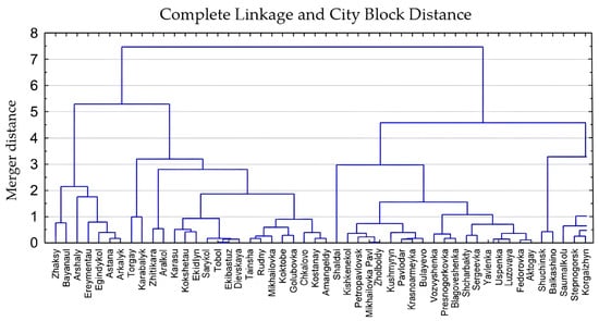
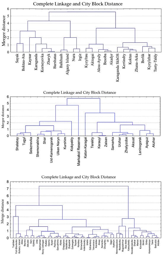
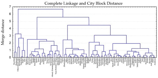
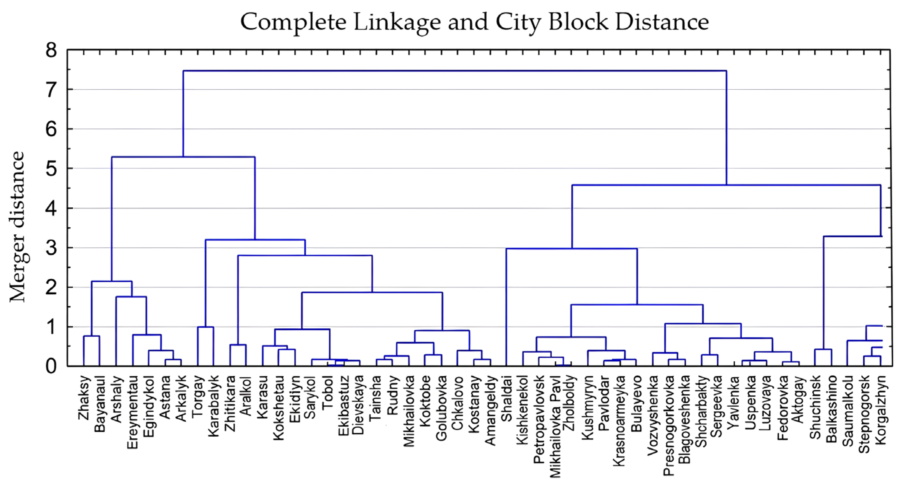
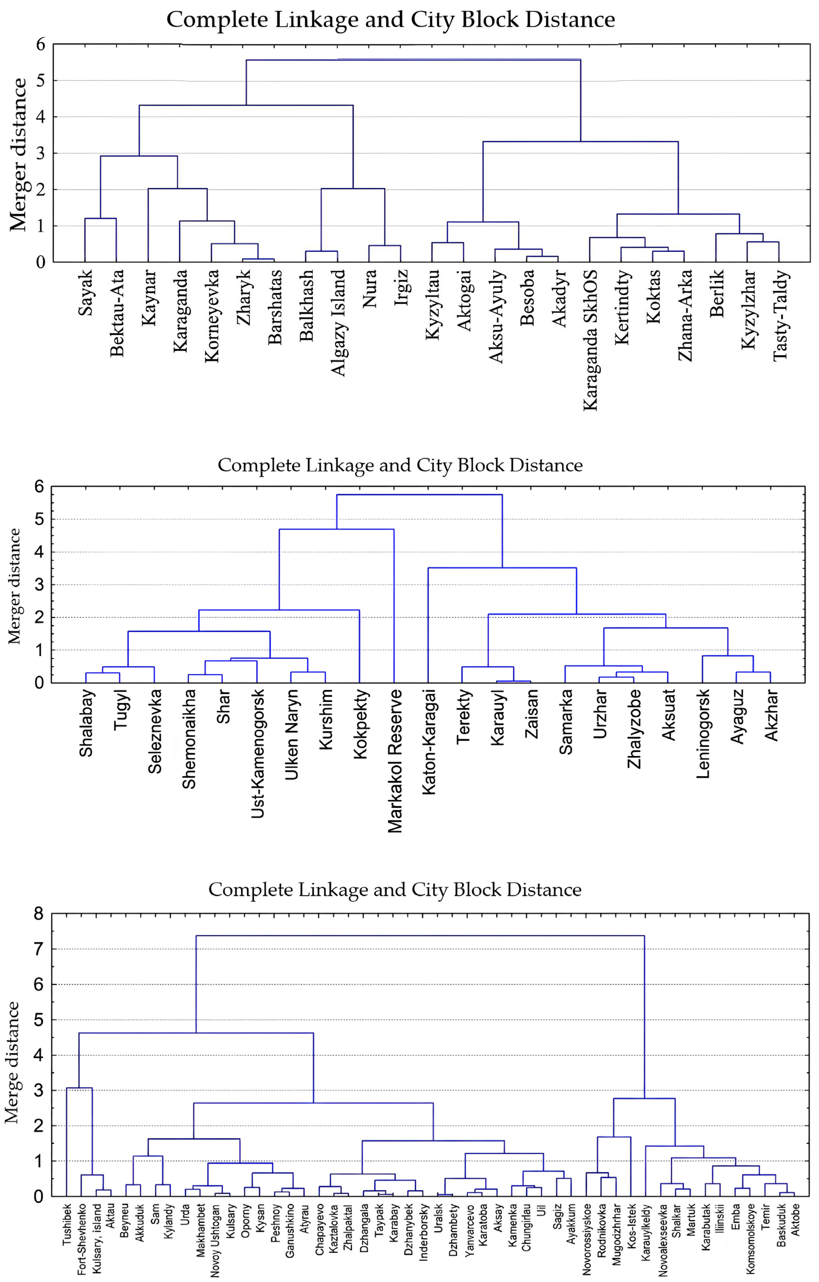
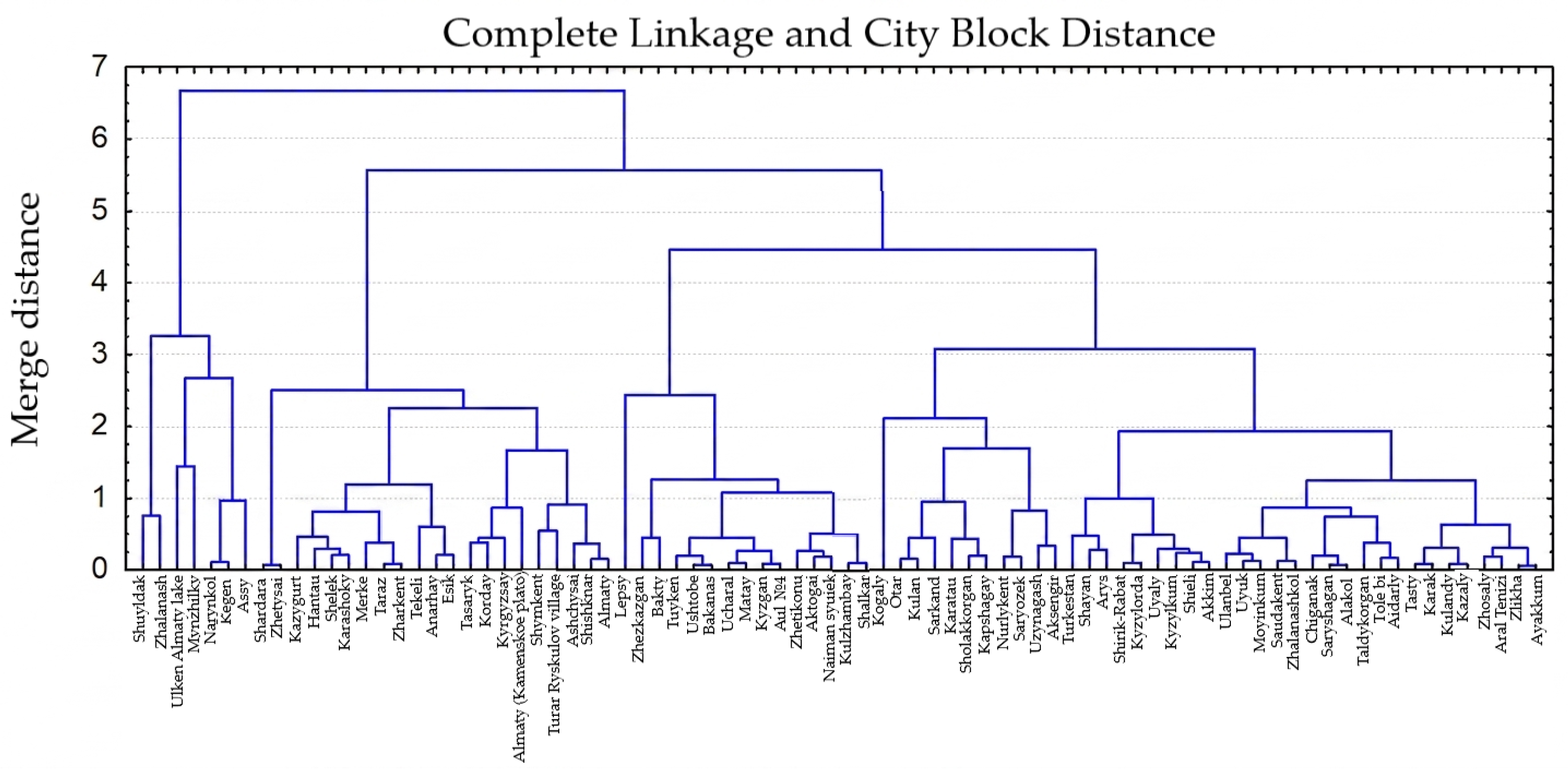
The ablation of stable snow cover typically occurs between the first ten-day period of March (in the south) and the first ten-day period of April (in the north and east), with terrain elevation remaining the primary governing factor in mountainous terrain. Based on the clustering results (incorporating elevation and absolute minimum temperature, °C), the Kazhydromet stations were classified into five distinct regional groups: Northern, Western, Central, Eastern, and combined Southern and Southeastern Kazakhstan. The final dendrograms illustrating this classification are presented in Figure 1.

Figure 1. Dendrograms of the regions of Kazakhstan.

Subsequently, utilizing the cluster-derived groups, the spatial distribution of snow loads was mapped across both the lowland and mountainous terrains of Kazakhstan.

3.1. Snow Load Distribution Across the Lowland Territory of Kazakhstan

Across lowland Kazakhstan, the timing of stable snow cover establishment varies distinctly with latitude. According to the dataset for the 1971–2020 period, stable snow cover forms, on average, on 13 November in the northern regions, 24 November in Central Kazakhstan, 30 November in Western Kazakhstan, 13 November in Eastern Kazakhstan, and 4 December in Southern and Southeastern Kazakhstan.

Three candidate station-level snow-load partitions were compared using Equations (1) and (2). Table 2, Table 3 and Table 4 give the actual class summaries used to calculate Table 5: Options 1, 2 and 3 contain 6, 11 and 9 classes, respectively, and use the same 210 station-level estimates. Classes are ordered by increasing snow load. The reported ranges are the minimum and maximum observed estimates within each class, not prescribed zoning thresholds; gaps between ranges reflect gaps in the observed station values.

Table 2. Candidate station-level snow-load partition—Option 1 (6 classes; n = 210).

Class	Number of Stations	Observed Snow-Load Range (kPa)	Sample Variance Di (kPa2)	Si with Next Class
1	76	0.4126–1.0470	0.029525	0.8062
2	107	1.0500–1.9780	0.057740	0.5725
3	15	2.0860–3.0400	0.081211	0.7601
4	5	3.1460–3.7970	0.065388	0.8125
5	5	4.1210–4.6640	0.044635	0.9762
6	2	5.8310–8.4110	3.328200	–

Table 3. Candidate station-level snow-load partition—Option 2 (11 classes; n = 210).

Class	Number of Stations	Observed Snow-Load Range (kPa)	Sample Variance Di (kPa2)	Si with Next Class
1	7	0.4126–0.5450	0.003256	0.9247
2	69	0.5530–1.0470	0.023012	0.7274
3	73	1.0500–1.5420	0.021265	0.6252
4	34	1.5510–1.9780	0.018120	0.6883
5	10	2.0860–2.4420	0.017113	0.7995
6	5	2.5770–3.0400	0.038384	0.8120
7	3	3.1460–3.5160	0.037233	0.5801
8	2	3.7100–3.7970	0.003784	0.9847
9	3	4.1210–4.4850	0.040036	0.3404
10	2	4.6060–4.6640	0.001682	0.9997
11	2	5.8310–8.4110	3.328200	–

Table 4. Candidate station-level snow-load partition—Option 3 (9 classes; n = 210).

Class	Number of Stations	Observed Snow-Load Range (kPa)	Sample Variance Di (kPa2)	Si with Next Class
1	47	0.4126–0.8370	0.012139	0.7674
2	58	0.8620–1.2490	0.012057	0.6981
3	44	1.2590–1.5420	0.008143	0.6894
4	28	1.5510–1.8490	0.010111	0.8298
5	16	1.8880–2.4420	0.030495	0.7601
6	6	2.5770–3.1460	0.062710	0.7778
7	4	3.4260–3.7970	0.029214	0.8992
8	5	4.1210–4.6640	0.044635	0.9762
9	2	5.8310–8.4110	3.328200	–

Table 5. Descriptive comparison of three candidate station-level snow-load partitions (n = 210). Lower k indicates smaller normalized dispersion; higher S_i indicates greater contrast relative to the lower-load class. S_i ranges are minima and maxima across adjacent pairs, not probabilities.

Candidate Partition (Number of Classes)	Normalized Dispersion Index k	Adjacent-Class Contrast Si (Min–Max)	Comparison with Uniform Reference
Option 1 (6)	0.736	0.573–0.976	Below reference (k < 1)
Option 2 (11)	1.092	0.340–0.9997	Above reference (k > 1)
Option 3 (9)	0.841	0.689–0.976	Below reference (k < 1)

Table 5 reports the recalculated descriptive diagnostics for the three worksheet partitions. The weighted within-class variances σw² are 0.080222, 0.052577 and 0.046532 kPa² for Options 1, 2 and 3, respectively. After normalization by the N-dependent reference in Equation (1), their k values are 0.736, 1.092 and 0.841. Thus Option 1 has the lowest normalized dispersion, whereas Option 3 has the lowest unnormalized weighted within-class variance.

Options 1 and 3 have normalized dispersion below the uniform reference (k < 1), whereas Option 2 exceeds it. The minimum adjacent-class contrast scores are 0.573, 0.340 and 0.689 for Options 1, 2 and 3, respectively; therefore, Option 3 has the highest minimum contrast among the evaluated pairs. For Option 2, the maximum score is 0.999660 (reported as 0.9997 in Table 5), which rounds to 1.0 at one decimal place. For its classes 10 and 11, l(C₁₀) = 0.029 kPa and l(C₁₀ ∪ C₁₁) = 1.57275 kPa, giving S₁₀ = 1 − (0.029/1.57275)² = 0.999660. Class 10 contains the close estimates 4.606 and 4.664 kPa, whereas class 11 contains 5.831 and 8.411 kPa. Thus the near-unit score reflects a small numerator relative to a union distance that also includes the substantial spread within class 11; it does not indicate certain boundary placement or uniformly compact classes.

These diagnostics compare candidate station-level classifications; they do not by themselves establish the geographical boundaries or design loads of the final nine-zone map. The station-level estimates span 0.4126–8.411 kPa. The map uses the zonal values described below, beginning at 0.8 kPa and including an open-ended highest class above 5.6 kPa; 5.6 kPa is therefore not an upper limit on station-level estimates or on the mapped highest class. The fact that Option 3 and the final map both contain nine groups does not establish a one-to-one correspondence between the calculated classes and mapped zones. The five-region lowland zoning described next uses a separate climatic indicator and geographical delineation. The diagnostic results should therefore not be interpreted as validation of the mapped zonal values or boundaries.

Kazakhstan was initially divided into five lowland snow regions using the long-term mean of the seasonal maximum snow water equivalent (SWE): Region 1, 20–40 mm; Region 2, 40–60 mm; Region 3, 60–80 mm; Region 4, 80–100 mm; and Region 5, more than 100 mm. These intervals classify a mean climatic indicator; they are not thresholds for the 50-year characteristic snow load. Boundaries were delineated with reference to landscape and physical-geographical maps, auxiliary maps and the calculated snow-cover indicators. Representative stations for the typological landscapes are listed in Table 6. Their seasonal maximum SWE distributions provided the basis for the characteristic ground snow load estimates with an annual exceedance probability of 0.02 summarized in Table 7.

Table 6. Distribution of reference stations by districts.

District	Benchmark Station (Climatic)
District 1	Atyrau, Kulsary, Akkuduk, Beineu, Aral Tenizi, Kazaly, Akkum, Balkhash, Moyynkum, Zharkent
District 2	Taipak, Wil, Zhezkazgan, Besoba, Mikhailovka (Pavlodar)
District 3	Kostanay, Torgay, Amangeldy
District 4	Petropavlovsk, Yavlenka, Ertis, Kamenka
District 5	Kokpekty, Mynzhylky, Rodnikovka

Table 7. Statistical parameters and representative characteristic ground snow loads at 2% annual exceedance probability for the five lowland snow regions.

Region	Coefficient of Variation (Cv)	Coefficient of Skewness (Cs)	Snow Load on the Ground—S kg/m2	Snow Load on the Ground—S kPa
1	0.76	1.52	90	0.9
2	0.53	1.59	120	1.2
3	0.40	1.80	150	1.5
4	0.49	1.47	200	2.0
5	0.39	1.56	>300	>3.0

Note: Region 5 represents an open-ended class corresponding to ground snow loads exceeding 300 kg/m² (3.0 kPa).

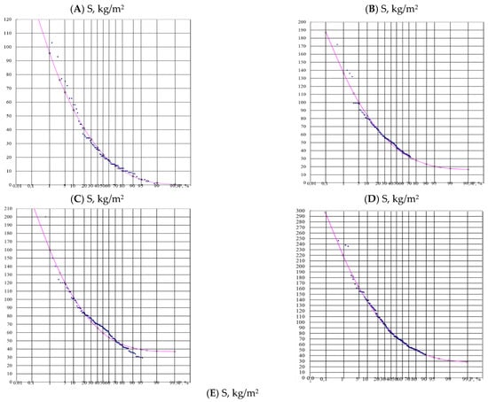
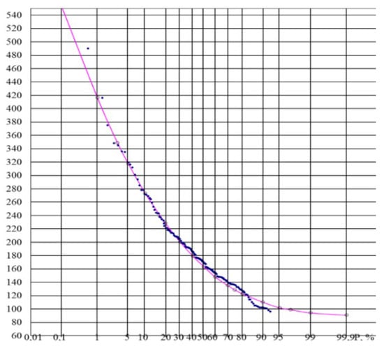
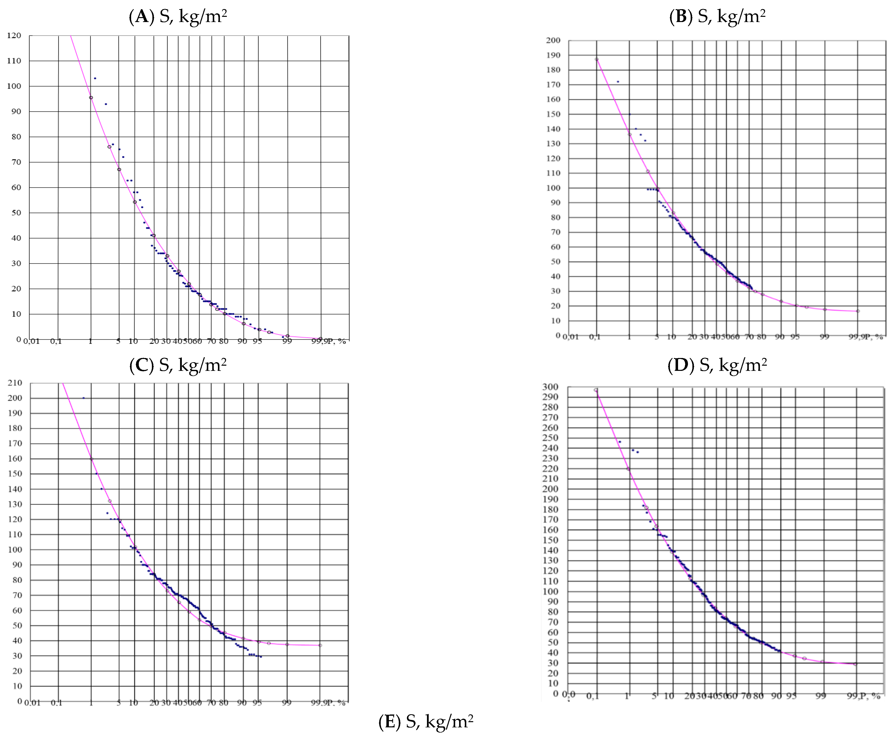
The empirical distribution of the maximum snow water equivalent (SWE) was approximated using reference stations for each of the five regions (Figure 2).

Figure 2. Snow load probability curves, 1971–2020. (A) Region 1; (B) Region 2; (C) Region 3; (D) Region 4; (E) Region 5.

Approximation of the empirical seasonal maximum SWE distributions by the probability-curve procedure described in Section 2 yielded the statistical parameters and representative characteristic ground snow load estimates for the five lowland regions (Table 7). These are upper-tail estimates at 2% annual exceedance probability, rather than the mean seasonal maximum SWE used to define the five-region intervals. The values 90, 120, 150, 200 and more than 300 in Table 7 are expressed as snow mass per unit area (kg/m²), with the corresponding loads given in kPa; they are not the regional mean SWE thresholds.

The borders were delineated based on landscape, physical-geographic, and auxiliary maps, while also incorporating all calculated snow cover climatic indicators.

Elevation-dependent ground snow load relationships were also established for the Kazakh Uplands, Mugalzhary and Kokshetau Upland (Table 8). These terrain units are considered within the lowland and hilly assessment. The regional regression datasets cover elevation intervals of 619–806, 177–372 and 155–398 m, respectively, in the Baltic Height System. Each relationship is applicable within the geographical unit and elevation interval specified in Table 8; these intervals do not define a common elevation threshold separating hilly and mountainous terrain.

Table 8. Regional ground snow load equations with a 2% annual exceedance probability for the upland and hilly territories of Central and Western Kazakhstan.

No.	Terrain Unit	Number of Stations	Regression Equation	Correlation Coefficient (R)	Standard Error of Estimate	F-Statistic	Elevation Ranges (m a.s.l.)	Ranges of Snow Load with 2% Exceedance Probability (kPa)
11	Kazakh Uplands	7 MS	S = 0.0061 × Z − 2.5831	0.923	0.21	28.9/6.6	619–806	1.16–2.44
22	Mugalzhary	8 MS	S = 0.0121 × Z − 1.0675	0.898	0.42	24.9/5.99	177–372	1.0–3.8
33	Kokshetau Upland	9 MS	S = 0.0049 × Z + 0.1937	0.88	0.225	24.8/5.56	155–398	1.0–2.6

For the Kazakh Uplands, the regional relationship is S = 0.0061Z − 2.5831, where S is the characteristic ground snow load (kPa) and Z is elevation (m) in the Baltic Height System [10,12]. This equation represents the Kazakh Uplands dataset at 619–806 m (Table 8); it is not a general relationship for mountainous zones.

3.2. Snow Load Distribution Across the Mountainous Territory of Kazakhstan

In mountainous regions, the timing of stable snow cover formation is strongly influenced by terrain elevation. The earliest stable snow cover at the reported stations is established on 20 October at Mynzhylky in Southeastern Kazakhstan (3017 m a.s.l.), on 1 November at Markakol Nature Reserve in Eastern Kazakhstan (1372 m a.s.l.), and on 22 November at Shuyldak in Southern Kazakhstan (1947 m a.s.l.). Ground snow loads in the mountain systems of Southern, Southeastern and Eastern Kazakhstan and adjacent territories were assessed using regional empirical relationships [25,26]. For the Altai region, data from six river basins, including the Ulba and Oba, were used; for Southern and Southeastern Kazakhstan, the relationships represent the Karatal and Boralday river basins and slopes of the Zhetysu Alatau, Iley Alatau and Karatau ranges (Table 9 and Table 10). The regression datasets in Table 9 cover regional elevation intervals within 300–3000 m, while those in Table 10 cover intervals within 477–2260 m in the Baltic Height System. Each equation is restricted to its tabulated regional and elevation range. These regression ranges describe the datasets used to establish the load–elevation relationships and are distinct from the elevations of stations cited above to illustrate snow-cover timing.

Table 9. Snow load equations with 2% probability used in zoning of Southern and South-Eastern Kazakhstan.

No.	Mountain System and River Basin	Number of Stations	Regression Equation	Correlation Coefficient (R)	Standard Error of Estimate	F-Statistic	Elevation Ranges (m a.s.l.)	Ranges of Snow Load with 2% Exceedance Probability (kPa)
11	Zhetysu Alatau Range, Karatal River	10 SMS	S = 0.0054 × Z − 3.90	0.98	0.569	223/5.3	1300–2700	3.12–10.68
22	Zhetysu Alatau Range, SW slope	4 MS	S = 0.0049 × Z − 0.694	0.95	0.62	18.3/18.5	300–1000	1.46–4.16
33	Iley Alatau Range, N slope	5 MS	S = 0.0014 × Z − 0.181	0.98	0.301	86.6/10.1	800–3000	0.94–4.02
44	Karatau Range, SW slope	5 MS	S = 0.0053 × Z − 1.80	0.99	0.36	272/10.1	600–1950	1.38–8.54
55	Boraldai River, Karatau Range, Boraldai Ridge	15 SMS	S = 0.0021 × Z + 0.462	0.89	0.237	51/4.67	700–1650	1.93–3.93

Table 10. Snow load equations with a 2% annual exceedance probability utilized for the zoning of Eastern Kazakhstan.

No.	Mountain System and River Basin	Number of Stations	Regression Equation	Correlation Coefficient (R)	Standard Error of Estimate	F-Statistic	Elevation Ranges (m a.s.l.)	Ranges of Snow Load with 2% Exceedance Probability (kPa)
1	Oba River, Oba Range	14 SMS	S = 0.0043 × Z − 1.2758	0.79	0.76	21/4.75	855–1599	2.4–5.6
2	Sharavka River, Oba Range	14 SMS	S = 0.0127 × Z − 3.6658	0.89	0.46	113/4.75	477–730	2.4–5.6
3	Berel River, Listvyaga Range	11 SMS	S = 0.0074 × Z − 6.3128	0.98	0.64	244/4.96	1177–1394	2.4–4.0
4	Kargyba River, Tarbagatai Range, N slope	14 SMS	S = 0.0049 × Z − 6.276	0.92	0.87	50.6/4.75	1770–2260	2.4–4.8
5	Ulba River, Ulbi Range	16 SMS	S = 0.0133 × Z − 6.155	0.91	2.26	69/4.67	643–884	2.4–5.6
6	Sarymsakty River, Sarymsakty Range	14 SMS	S = 0.0055 × Z − 7.6123	0.70	1.53	10.5/4.84	1820–2111	2.4–4.0

Based on the zoning results, a ground snow load zoning map for the territory of the Republic of Kazakhstan was developed in accordance with Eurocode 1 [3,6].

Nine ground snow load zones are identified on the national map (Table 11). The five-region scheme in Table 7 provides a preliminary lowland climatic framework and representative characteristic-load estimates. The national map extends the assessment to both lowland and mountain terrain, bringing together the spatial distribution of station-based characteristic loads and the regional elevation-dependent relationships described above. Its nine class values are those assigned to the mapped zones, rather than numerical transformations of the five representative values in Table 7. Thus, the five-region and nine-zone schemes serve different spatial purposes and do not imply a one-to-one correspondence or a fixed conversion of 0.9, 2.0 or more than 3.0 kPa into particular national map classes.

Table 11. Snow load distribution across the territory of Kazakhstan.

Snowy Regions of the Republic of Kazakhstan	1	2	3	4	5	6	7	8	9
S, kPa (kg/m2)	0.8 (80)	1.2 (120)	1.5 (150)	1.8 (180)	2.4 (240)	3.2 (320)	4.0 (400)	4.8 (480)	>5.6 (>560)
Relief	Flat and hilly					Mountain

Note: Zone 9 (>5.6 kPa, corresponding to >560 kg/m² under the approximate conversion convention used here) is an open-ended ground snow load class. The value 5.6 kPa is its lower threshold, not an assigned load or an upper cap. A numerical characteristic ground snow load within this class is obtained from the applicable regional elevation relationship within its tabulated geographical and elevation limits. The map class alone does not specify a single load for all locations within Zone 9.

The resulting snow load zoning map and regional elevation-dependent relationships provide a unified framework for describing the spatial distribution of characteristic ground snow loads across Kazakhstan. The nine zones presented in Table 11 capture regional differences in snow loading, while the regression equations quantify its variation with elevation within the investigated regions. Together, these results characterize both the geographical and altitudinal differentiation of ground snow loads and provide a basis for updating national snow load provisions.

4. Discussion

4.1. Regional Differentiation and the Contribution of Elevation-Dependent Assessment

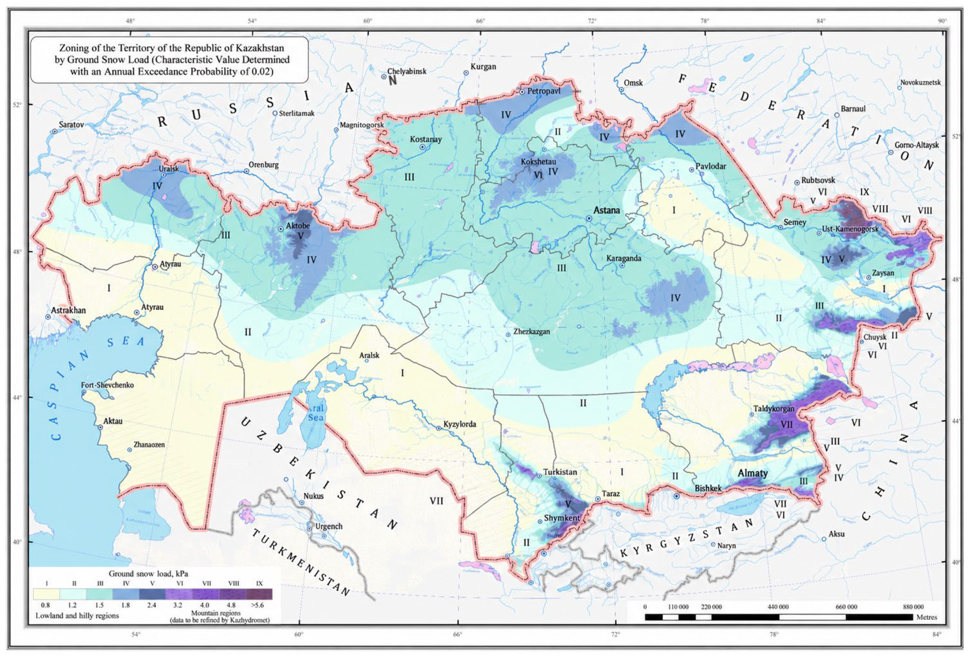
The results establish a national framework for snow-load assessment that combines the climatic differentiation of Kazakhstan with the influence of terrain elevation. The regional contrasts in snow-cover characteristics reported in Table 1 and the ground-load classes shown in Figure 3 demonstrate the importance of representing both broad climatic gradients and differences within mountain systems. Integrating these two spatial scales is a central contribution of the study: regionalization describes the geographical organization of snow conditions, while the elevation relationships provide a quantitative basis for assessing loads within individual terrain units.

Figure 3. Ground snow load zoning of the territory of the Republic of Kazakhstan with an annual exceedance probability of 0.02.

The use of SWE gives the assessment a direct physical connection to snow mass per unit area. This is important because differences in snow depth do not necessarily imply equivalent differences in snow load. Sturm et al. [27] showed that bulk snow density varies with snow depth, season, and snow climate. The use of snow surveys and the associated snow-cover measurements therefore provides a stronger basis for load assessment than a classification based on snow depth alone.

The regression relationships in Table 8, Table 9 and Table 10 further demonstrate that the response of snow load to elevation differs among the investigated mountain systems and basins. The contrasting coefficients for the Karatal basin, the Iley Alatau, and the eastern mountain systems support regional differentiation of elevation corrections. This approach develops the methodological line established in the studies of southern, southeastern, and eastern Kazakhstan and brings the regional relationships together within a national zoning framework. The scientific contribution lies in this integration of long-term observations, regional classification, elevation-dependent assessment, and spatial representation.

4.2. Comparison with Earlier Kazakhstan Zoning and the Russian 2008 Framework

Vorgina’s earlier five-zone scheme, described in the regional publications [28,29], established an important foundation for the assessment of snow-cover weight in Kazakhstan. The present study retains the principle of regional differentiation and develops it through the use of the 1971–2020 observation period, statistical regionalization, elevation relationships, and a national map of characteristic ground snow loads. The transition from the earlier five-zone lowland scheme to a nine-class national map expands the spatial representation to include both lowland and mountain conditions within a common assessment framework.

A fundamental distinction concerns the target exceedance probability. The earlier map represented snow-cover weight with an annual exceedance probability of 0.20, corresponding to a mean return period of 5 years, whereas the present assessment uses 0.02, corresponding to 50 years. The revised statistical basis allows less frequent, more severe snow conditions to be represented in the load assessment. Differences between the two maps consequently reflect both the adopted probability level and the updated observational and spatial framework. This distinction is essential when interpreting the evolution of snow-load zoning and separating methodological advances from changes in the snow-cover regime.

The Russian 2008 framework provides a useful comparison of the numerical load classes. STO 36554501-015-2008, developed with participation from the Voeikov Main Geophysical Observatory, specifies eight ground snow-weight values: 0.8, 1.2, 1.8, 2.4, 3.2, 4.0, 4.8, and 5.6 kPa [30]. The Kazakhstan map uses a comparable sequence, with an additional 1.5 kPa class and an open-ended highest class greater than 5.6 kPa. These features preserve comparability of the numerical grading while representing the range of conditions identified for Kazakhstan. The probability criteria nevertheless require explicit distinction: Section 5.2 of the Russian document uses a 25-year annual-maximum criterion for determinations in mountainous and insufficiently studied areas, whereas the present study adopts a 50-year criterion [30].

This comparison places the Kazakhstan results within the wider development of snow-load assessment in the region. It establishes similarities in the grading of loads and differences in the probabilistic basis and spatial differentiation. A further comparison of adjacent territories using matched border stations and a common probability criterion would extend the analysis to the continuity of snow-load fields across the Kazakhstan–Russia border.

4.3. Methodological Advances and Engineering Significance

The proposed approach connects long-term hydrometeorological observations with the characteristic-value framework of Eurocode 1 [3]. Its engineering significance follows from the combination of a defined annual exceedance probability, spatially differentiated load classes, and quantitative elevation relationships. Together, these elements provide an observational and statistical basis for updating snow-load provisions for Kazakhstan and assigning loads in accordance with regional conditions.

European standards (Eurocode 1) are generally based on the same methodological principles but exhibit several significant differences:

• Instead of the standard snow load value (mean annual maximum), a characteristic value corresponding to a 50-year mean return period is utilized;
• More detailed zoning of snow loads across both lowland and mountainous terrains is introduced by establishing elevation-dependent relationships;
• The territory of Kazakhstan is divided into 9 zones: I—0.8 kPa, II—1.2 kPa, III—1.5 kPa, IV—1.8 kPa, V—2.4 kPa, VI—3.2 kPa, VII—4.0 kPa, VIII—4.8 kPa, and IX—greater than 5.6 kPa;
• The service life of conventional buildings is taken into account (the service life for Class 4 structures under the RK SP building code is 50 years).

The national differentiation achieved here is consistent with the purpose of Eurocode National Annexes, which adapt the shared framework to national climatic conditions. Croce et al. [5] explain that the European ground snow-load map in informative Annex C was developed to support national mapping and improve consistency among countries. The Kazakhstan results follow this principle by combining a common characteristic-value criterion with load classes and regional elevation relationships derived for the country’s own climatic and topographic setting. The scientific and practical value therefore lies in the adaptation of the probabilistic framework through national observational evidence.

The combined use of the zoning map and regional elevation relationships is especially relevant in mountain basins, where calculated loads can vary substantially over relatively short distances. For the Karatal basin, the relationship in Table 9 gives characteristic ground snow loads of 3.12–10.68 kPa over 1300–2700 m. The value 10.68 kPa is the estimate at the upper end of this studied elevation interval, not a universal upper limit for mountain regions. Zone IX (>5.6 kPa) groups high-load areas without truncating their regional estimates at 5.6 kPa. No upper cap on characteristic ground snow loads is introduced in this assessment. For engineering application, the applicable regional relationship provides a numerical ground-load estimate at the elevation of the location under consideration, within the stated geographical and elevation limits. Locations outside these limits require a separate local assessment rather than extrapolation of the tabulated equations. The assessed quantities are characteristic ground snow loads; determination of roof loads and structural design values requires a separate calculation under the applicable structural design provisions [3].

The resulting framework supports the revision of national snow-load provisions, the selection of regionally appropriate ground-load inputs for structural design, and the identification of areas requiring particular attention because of elevated snow loads. Its contribution is a consistent connection between measured snow conditions, statistically defined characteristic values, and the spatial differentiation needed for engineering application.

4.4. Limitations and Priorities for Further Development

The characteristic loads are upper-tail estimates derived from finite records. A 50-year return period denotes an annual exceedance probability of 0.02; it does not imply that an event of that magnitude must occur once within a 50-year observational period. Estimation uncertainty depends on the number of observed seasonal maxima, record completeness and homogeneity, and the adopted probability curve. Short records provide less information about the upper tail. Analogue-based reconstruction introduces additional uncertainty, and a supplemented series should not be treated as an equivalent number of independently observed seasons. Station-specific confidence intervals, propagation of re-construction uncertainty and formal goodness-of-fit statistics for the adopted curves were not quantified in this assessment. Graphical agreement therefore does not establish statistical acceptance of a distribution. The loads should be interpreted as point estimates conditional on the adopted fitting procedure. Station exposure, the timing of snow surveys and the regional applicability of the elevation equations provide further limitations. Quantifying interval uncertainty and testing sensitivity to reconstruction and distribution choice are priorities for further assessment.

The sensitivity of the preliminary climatic grouping to the choice of clustering variables was not evaluated. Comparing the adopted H–T_abs.min combination with alternative sets incorporating SWE, snow depth, and stable snow-cover duration would help assess the robustness of the grouping and its implications for subsequent snow-load regionalization.

Observations of snow depth, snow density, and snow water equivalent (SWE) provide the empirical basis for estimating characteristic ground snow loads and establishing regional relationships; they do not constitute an independent validation dataset. No stations or observation periods were withheld for independent validation. Agreement between the fitted curves and the observations used to derive them, together with the classification diagnostics, characterizes within-sample consistency rather than out-of-sample predictive performance. The results establish an observation-based national framework for ground snow load zoning. Figure 3 illustrates the spatial distribution of snow-load classes without quantifying their respective shares of the national territory.

Further development can build on the national framework established in this study. Schellander et al. [31] demonstrate how cross-validation can be used to assess the predictive performance of spatial snow-load estimates, providing a methodological reference for subsequent validation of the Kazakhstan map. The JRC report by Croce et al. [32] also highlights the importance of evaluating climate-change effects in terms of characteristic climatic actions. Extending the historical assessment through subperiod comparisons and climate-informed analysis would therefore strengthen its use in the periodic revision of national snow-load provisions. The present observational database, map, and regional relationships provide the basis for these extensions.

5. Conclusions

Within the scope of this study, zoning of the territory of Kazakhstan was performed based on a snow cover weight with an annual exceedance probability of 0.02 (a 50-year return period), and a snow cover weight distribution map covering the entire territory of Kazakhstan was constructed, delineating 9 distinct zones. The primary datasets comprised observational records from 210 meteorological stations for the period 1971–2020 and snow survey data from 17 mountainous river basins. The snow-cover regime was investigated throughout Kazakhstan. The regional elevation-dependent ground snow load relationships presented in Table 8, Table 9 and Table 10 collectively cover elevations from 155 to 3000 m in the Baltic Height System, with each equation applicable within its own tabulated geographical unit and elevation interval. Relationships among snow-load characteristics, elevation, and regional conditions were subsequently established.

This study demonstrates an innovative approach to assessing snow loads in accordance with Eurocode 1 (EN 1991-1-3:2003) across Kazakhstan, addressing the limitations of the outdated SNiP 2.01.07-85 codes, such as insufficient spatial detail and the neglect of topography and elevation. The developed methodology, integrating empirical–statistical methods, cluster and regression analyses, and GIS technologies (ArcGIS 10.5, ArcMap) [27,28], enabled the update of snow load maps using long-term data from 210 meteorological stations of the RSE “Kazhydromet,” while considering spatial snow-cover variability, qualitative terrain grouping by exposure and shelter, and regional climatic factors.

The key findings demonstrate substantial regional differentiation in characteristic ground snow loads, as represented by the nine-zone map (Figure 3 and Table 11). The map includes zones assigned 1.2 and 1.5 kPa and higher-load zones assigned 2.4 and 3.2 kPa, as well as mountain classes of 4.0, 4.8 and greater than 5.6 kPa. Relative to the previous three-zone scheme (0.5–1.0 kPa), the proposed zoning provides more detailed spatial differentiation and adopts an annual exceedance probability of 0.02 (a 50-year mean return period). The regional regression relationships quantify the elevation dependence of ground snow loads within the investigated terrain units and complement the national zoning map.

The proposed zoning maps delineate nine snow-load zones with characteristic ground snow loads ranging from 0.8 to an open-ended highest class exceeding 5.6 kPa, including five zones for lowland areas and four for mountain slopes. The developed algorithms and zoning results can be used to update national building codes, support structural design and emergency risk assessment, harmonize Kazakhstan’s standards with European norms, and enhance infrastructure safety across Central Asia. For future research, expanding the database with satellite observations and climate modeling is recommended to account for global warming trends, along with integration into early warning systems for extreme snow anomalies. These findings establish a baseline for analogous studies in neighboring regions with unstable snow cover, supporting sustainable infrastructure development. The highest class is open-ended: numerical characteristic ground snow loads are resolved using the applicable regional elevation relationships within their tabulated limits, and are not capped at 5.6 kPa.

It should be noted that the obtained results carry practical significance not only for structural design but also for the hydrological assessment of flood hazards. According to the developed zoning, the maximum snow water equivalent (SWE) varies from 106 mm in southern regions to 230 mm in Eastern Kazakhstan, indicating a more than twofold regional discrepancy in potential snowmelt runoff volumes. Given that approximately 90% of Kazakhstan’s annual river runoff is generated during the spring season, spatial data on snow storage serves as a crucial foundation for forecasting spring freshets and evaluating snowmelt flood risks. The developed snow load and SWE maps can be seamlessly integrated into hydrological modeling and emergency early warning systems, which is highly relevant for the northern, eastern, and mountainous regions of the country that are most vulnerable to spring flooding.

References

- Croce, P.; Formichi, P.; Landi, F.; Mercogliano, P.; Bucchignani, E.; Dosio, A.; Dimova, S. The snow load in Europe and the climate change. Clim. Risk Manag. 2018, 20, 138–154. [Google Scholar] [CrossRef] [Scilit]
- Agency for Construction and Housing and Communal Services of the Republic of Kazakhstan. Methodological Guidelines for Processing Climatic Parameters for the Design Observation Period and Compiling Maps of Climatic Parameters for SN RK EN 1991-2007/2011 “Actions on Structures”; Agency for Construction and Housing and Communal Services of the Republic of Kazakhstan: Astana, Kazakhstan, 2012. (In Russian) [Google Scholar]
- Agency for Construction and Housing and Communal Services of the Republic of Kazakhstan. Building Codes SN RK EN 1991-1-3:2003/2011 “Actions on Structures.” Part 1–3: General Actions—Snow Loads; Agency for Construction and Housing and Communal Services of the Republic of Kazakhstan: Astana, Kazakhstan, 2011. (In Russian) [Google Scholar]
- State Construction Committee. Building Codes and Regulations, SNiP 2.01.07-85*: Loads and Actions; State Construction Committee: Moscow, Russia, 2001. (In Russian) [Google Scholar]
- Croce, P.; Formichi, P.; Landi, F.; Marsili, F. Harmonized European ground snow load map: Analysis and comparison of national provisions. Cold Reg. Sci. Technol. 2019, 168, 102875. [Google Scholar] [CrossRef] [Scilit]
- EN 1991-1-3:2003; Eurocode 1: Actions on Structures—Part 1–3: General Actions—Snow Loads. European Committee for Standardization (CEN): Brussels, Belgium, 2003.
- ISO 4355:2013; Bases for Design of Structures—Determination of Snow Loads on Roofs. International Organization for Standardization (ISO): Geneva, Switzerland, 2013.
- Assunção, R.M.; Neves, M.C.; Câmara, G.; da Costa Freitas, C. Efficient regionalization techniques for socio-economic geographical units using minimum spanning trees. Int. J. Geogr. Inf. Sci. 2006, 20, 797–811. [Google Scholar] [CrossRef] [Scilit]
- Guo, D. Regionalization with dynamically constrained agglomerative clustering and partitioning (REDCAP). Int. J. Geogr. Inf. Sci. 2008, 22, 801–823. [Google Scholar] [CrossRef] [Scilit]
- Kozhakhmetov, P.Z.; Eleuova, K.T.; Baymagambetov, B.O.; Nurbatsina, A.A. Distribution of ground snow loads in the mountainous territories of Eastern Kazakhstan. Hydrometeorol. Ecol. 2015, 1, 8–20. (In Russian) [Google Scholar]
- Pavlova, I.A.; Podrezov, O.A.; Podrezov, A.O. Maximum snow water equivalent and snow loads in the territory of Kyrgyzstan. Vestn. KRSU 2011, 11, 160–166. (In Russian) [Google Scholar]
- Kozhakhmetov, P.Z.; Eleuova, K.T.; Baymagambetov, B.O.; Nurbatsina, A.A. Distribution of ground snow loads in the mountainous territories of southern and southeastern Kazakhstan. Hydrometeorol. Ecol. 2014, 4, 7–20. (In Russian) [Google Scholar]
- Institute of Geography of the Republic of Kazakhstan. National Atlas of the Republic of Kazakhstan: Vol. 1. Natural Conditions and Resources; Institute of Geography of the Republic of Kazakhstan: Almaty, Kazakhstan, 2010. (In Russian) [Google Scholar]
- Main Directorate of Geodesy Cartography. Atlas of the, U.S.S.R.; Main Directorate of Geodesy Cartography: Moscow, Russia, 1984. (In Russian) [Google Scholar]
- Kaufman, L.; Rousseeuw, P.J. Finding Groups in Data: An Introduction to Cluster Analysis; John Wiley & Sons: Hoboken, NJ, USA, 1990. [Google Scholar] [CrossRef] [Scilit]
- Kobysheva, N.V.; Narovlyansky, G.Y. Climatological Processing of Meteorological Information; Gidrometeoizdat: Leningrad, Russia, 1978; 295p. (In Russian) [Google Scholar]
- Kobysheva, N.V. (Ed.) Climatic Parameters for Building Design: Reference Guide to SNiP 23-01-99 “Building Climatology”; Gidrometeoizdat: St. Petersburg, Russia, 2008; 182p. (In Russian) [Google Scholar]
- Lundquist, J.D.; Pepin, N.; Rochford, C. Automated algorithm for mapping regions of cold-air pooling in complex terrain. J. Geophys. Res. Atmos. 2008, 113, D22107. [Google Scholar] [CrossRef] [Scilit]
- Prim, R.C. Shortest connection networks and some generalizations. Cybern. Collect. 1961, 2, 95–107. (In Russian) [Google Scholar]
- Kruskal, J.B. On the shortest spanning subtree of a graph and the traveling salesman problem. Proc. Am. Math. Soc. 1956, 7, 48–50. [Google Scholar] [CrossRef] [Scilit]
- Zahn, C.T. Graph-Theoretical Methods for Detecting and Describing Gestalt Clusters. IEEE Trans. Comput. 1971, C-20, 68–86. [Google Scholar] [CrossRef] [Scilit]
- Kobysheva, N.V. (Ed.) Guide to Specialized Climatological Services for the Economy; Voeikov Main Geophysical Observatory: St. Petersburg, Russia, 2008; Chapter 2. (In Russian) [Google Scholar]
- Ahmed, K.; Shahid, S.; Ismail, T.; Nawaz, N.; Wang, X.-J. Absolute homogeneity assessment of precipitation time series in an arid region of Pakistan. Atmósfera 2018, 31, 301–316. [Google Scholar] [CrossRef] [Scilit]
- Gumbel, E.J. Statistics of Extremes; Columbia University Press: New York, NY, USA, 1958. [Google Scholar] [CrossRef] [Scilit]
- Pigoltsina, G.B. Justification of the need and principles of accounting for meso- and microclimate in comprehensive assessments of natural resources for various sectors of the economy. Tr. Gl. Geofiz. Obs. A.I. Voeikova 2009, 89–115. (In Russian) [Google Scholar]
- Narovlyansky, G.Y. Climatology, Part I: Methods of Climatological Processing of Meteorological Observations with Elements of Mathematical Statistics; Gidrometeoizdat: St. Petersburg, Russia, 1964. (In Russian) [Google Scholar]
- Dobesch, H.; Dumolard, P.; Dyras, I. (Eds.) Spatial Interpolation for Climate Data: The Use of GIS in Climatology and Meteorology; ISTE: London, UK, 2007. [Google Scholar] [CrossRef] [Scilit]
- López-Moreno, J.I.; Vicente-Serrano, S.M.; Lanjeri, S. Mapping snowpack distribution over large areas using GIS and interpolation techniques. Clim. Res. 2007, 33, 257–270. [Google Scholar] [CrossRef] [Scilit]
- Sturm, M.; Taras, B.; Liston, G.E.; Derksen, C.; Jonas, T.; Lea, J. Estimating snow water equivalent using snow depth data and climate classes. J. Hydrometeorol. 2010, 11, 1380–1394. [Google Scholar] [CrossRef] [Scilit]
- STO 36554501-015-2008; Loads and Actions. Sections 5.1–5.2, Table 5.1 and Appendix Zh. Research Center for Construction: Moscow, Russia, 2008. Available online: https://meganorm.ru/Data2/1/4293831/4293831654.htm (accessed on 15 June 2026). (In Russian)
- Schellander, H.; Winkler, M.; Hell, T. Towards a reproducible snow load map—An example for Austria. Adv. Sci. Res. 2021, 18, 135–144. [Google Scholar] [CrossRef] [Scilit]
- Bucchignani, E.; Croce, P.; Dimova, S.; Dosio, A.; Formichi, P.; Landi, F.; Mercogliano, P. Towards a New European Snow Load Map; EUR 28149 EN; Publications Office of the European Union: Luxembourg, 2016. [Google Scholar] [CrossRef]
Disclaimer/Publisher’s Note: The statements, opinions and data contained in all publications are solely those of the individual author(s) and contributor(s) and not of MDPI and/or the editor(s). MDPI and/or the editor(s) disclaim responsibility for any injury to people or property resulting from any ideas, methods, instructions or products referred to in the content. |
© 2026 by the authors. Licensee MDPI, Basel, Switzerland. This article is an open access article distributed under the terms and conditions of the Creative Commons Attribution (CC BY) license.