


Abstract
Leaf water content (LWC) is a key physiological indicator for assessing crop water status. However, its spectral response may vary under different irrigation practices, which limits the general applicability of existing models. This study aims to develop irrigation-specific LWC estimation models for spring wheat based on UAV multispectral imagery. Field experiments were conducted during two growing seasons (2023–2024) under three irrigation methods, with five water treatments and three replicates, resulting in a total of 45 experimental plots. Multispectral data and in situ measurements were collected at key growth stages. Irrigation-dependent sensitive vegetation indices were identified through correlation analysis, and machine learning models, including Random Forest (RF), Multiple Linear Regression (MLR), and Backpropagation Neural Network (BPNN), were constructed and evaluated using a five-fold cross-validation framework. The results showed that spectral sensitivity to LWC varied significantly across irrigation methods, with different dominant indicators under FD, ND, and MD. Model performance also exhibited irrigation-dependent differences. Among the three models, RF showed the most stable performance, achieving mean R2 values of 0.70, 0.74, and 0.62 and corresponding RMSE values of 0.04, 0.06, and 0.08 under FD, ND, and MD, respectively. In contrast, MLR showed lower predictive accuracy, while BPNN exhibited limited robustness under the current dataset, particularly under ND. These findings highlight the importance of irrigation-specific modeling strategies for improving LWC estimation reliability.
1. Introduction
Efficient crop water monitoring is fundamental to irrigation management in arid and semi-arid regions, where agricultural production depends strongly on artificial water supply. Among various crop water-related traits, leaf water content is a direct physiological indicator of plant water status because it reflects the balance between water uptake, transport, and transpiration within plant tissues. Compared with soil-based indicators, such as soil moisture content or soil water potential, LWC is more closely related to the actual physiological response of crops to water deficit. However, conventional determination of crop water status still relies heavily on field sampling, oven drying, and manual measurements, which are labor-intensive, time-consuming, and difficult to implement for large-scale, high-frequency monitoring [1,2]. Therefore, rapid and non-destructive approaches for monitoring crop water status are urgently needed for water-saving agricultural management [3,4,5,6,7].
With the rapid development of remote sensing technologies and sensor miniaturization, UAV platforms have become important tools for large-scale crop phenotyping. Equipped with LiDAR, RGB, multispectral, hyperspectral, and thermal infrared sensors, UAVs can provide high-resolution spatial and temporal data for estimating structural, physiological, and biochemical crop traits, including plant height, canopy coverage, biomass, chlorophyll content, and water-related parameters [3,5,8]. Among these sensing approaches, multispectral imagery has been widely used in agricultural monitoring because of its relatively low cost and practical applicability in field conditions.
The theoretical basis of remote sensing-based crop water monitoring lies in the interaction between electromagnetic radiation and crop canopies. Changes in crop water status can influence leaf optical properties, canopy structure, and vegetation reflectance, thereby affecting spectral indices derived from visible, near-infrared, and red-edge bands. Numerous studies have shown that vegetation indices and machine learning models can be used to estimate crop water status and drought response in wheat and other crops [6,9,10,11]. Recent studies have further indicated that UAV-based crop water monitoring is evolving toward multi-sensor integration, advanced machine learning, and improved model robustness under complex field conditions [12,13]. Machine learning algorithms such as Support Vector Machines, Random Forest, and neural networks exhibit strong capabilities in modeling nonlinear relationships between spectral features and crop water parameters. At the same time, modern irrigation monitoring and decision-making systems are increasingly integrating sensor networks, evapotranspiration (ET)-based scheduling, thermal infrared sensing, and multi-source data fusion, indicating that precision irrigation is gradually moving toward more intelligent and data-driven frameworks.
Nevertheless, several important limitations remain in existing studies. First, many UAV-based studies on wheat water status estimation have focused on general modeling frameworks under a single irrigation condition, without explicitly considering how different irrigation methods may influence canopy spectral response. Second, broad-band multispectral indices may suffer from reduced sensitivity or saturation under dense canopies, and empirical models developed under one set of field conditions may show limited transferability across seasons, irrigation regimes, or experimental sites. Third, temporal variability in crop growth stages, management practices, and environmental conditions introduces uncertainty into water status estimation, which poses challenges for model robustness and generalization. Although advanced modeling approaches based on deep learning, hyperspectral sensing, thermal infrared sensing, and data fusion are increasingly being explored, these approaches may not always be easily transferable to routine field applications because of their higher cost, complexity, and data requirements.
For spring wheat production in arid regions, irrigation management is not only determined by irrigation amount, but also by irrigation method. Different irrigation systems may vary in water application pattern, wetted soil distribution, evaporation control, application efficiency, and root-zone water supply. Recent irrigation engineering studies have shown that irrigation equipment design and operating parameters can substantially influence field water distribution uniformity and water application efficiency under arid conditions, thereby affecting crop water supply and response [14]. These differences can further affect canopy development, crop physiological response, and the relationship between spectral indices and LWC. For example, film mulching can reduce surface evaporation and modify the soil hydrothermal regime, while shallow-buried drip irrigation may change the spatial pattern of soil wetting compared with conventional drip irrigation. Consequently, models developed under one irrigation condition may not be directly applicable to other irrigation methods. However, irrigation-specific analyses of LWC-sensitive spectral indicators and estimation models for spring wheat remain insufficiently explored, particularly in inland arid regions.
Against this background, this study focused on spring wheat grown under three irrigation methods, FD, ND, and MD, combined with multiple water treatments. The objectives of this study were to: (1) identify spectral indicators sensitive to LWC under different irrigation methods; (2) compare the performance of different machine learning models for LWC estimation under contrasting irrigation conditions; and (3) explore the necessity of irrigation-specific modeling for spring wheat LWC estimation in an arid-region production system. By addressing these questions, this study aimed to provide methodological support for UAV-based crop water status monitoring and to improve the understanding of spectral–water response mechanisms under different irrigation practices.
2. Materials and Methods
2.1. Study Area
The field experiments were conducted during 2023–2024 at the Shiyanghe Experimental Station of China Agricultural University (37°52′ N, 102°50′ E; altitude 1581 m), located in Wuwei City, Gansu Province, Northwest China. This region is a typical inland arid area, with a temperate arid continental climate and abundant solar radiation. The average annual sunshine duration exceeds 3000 h, and the mean annual temperature is approximately 8 °C. The region is characterized by a large diurnal temperature range, which is conducive to dry matter accumulation. However, it suffers from severe water shortage because of low precipitation. The long-term mean annual precipitation is 164 mm, while the annual surface evaporation is approximately 2000 mm. The groundwater depth ranges from 40 to 50 m, and agricultural production heavily relies on irrigation. The soil is sandy, with an average soil bulk density of 1.56 g cm−3 within the 1 m soil profile and a field capacity 0.09 cm3 cm−3.
2.2. Experimental Design
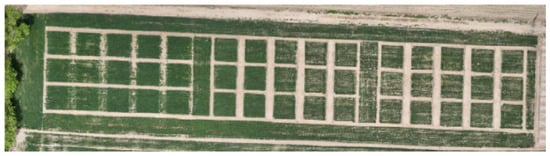
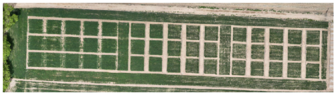
Spring wheat was selected for experiments conducted from March to August in both 2023 and 2024. Its growth period was divided into six stages: the seedling stage, the tillering stage, the jointing stage, the heading stage, the grain-filling stage, and the maturity stage. Three irrigation methods were established: plastic film-mulched drip irrigation (FD), non-mulched drip irrigation (ND), and non-mulched shallow-buried drip irrigation (MD). Each method was designed with five irrigation treatments: CK (80% of field capacity, FC), W1 (90% of CK), W2 (80% of CK), W3 (70% of CK), and W4 (60% of CK), where CK represented the full irrigation treatment. The irrigation design was based on field-capacity-controlled water regulation commonly used in local field irrigation experiments. CK represented the local full irrigation treatment under the experimental conditions, whereas W1–W4 were established as relative gradients to generate contrasting water supply levels under each irrigation method. Each treatment was replicated three times. Each plot measured 5 m × 5.4 m (27 m2). The field layout is illustrated in Figure 1.
Figure 1.
Field layout schematic of the experiment.
The spring wheat cultivar was “Yongliang 4.” The row spacing was set at 15 cm, with 36 rows per plot. The seeding density was approximately 6.0 × 10⁶ seeds ha−1. For the FD treatment, sowing was conducted using a precision hole seeder, while under ND and MD treatments, a drill seeder was applied. Drip irrigation belts were arranged in a “one pipe for two rows” pattern, with a spacing of 30 cm between belts. Each plot contained 18 drip lines, each being 5.2 m long. The discharge rate of the emitter was 3 L h−1, and its spacing was 150 mm. The sowing was conducted on 30 March in both years. The harvest dates were 26 July 2023 (growth duration: 119 days) and 14 July 2024 (growth duration: 107 days). Total irrigation amounts during the growth period are presented in Table 1.
Table 1.
Total irrigation amount during the growth period across treatments.
Fertilizer application was consistent in both years. In 2023, urea (900 kg ha−1) was applied with the initial irrigation on 8 May, and 600 kg ha−1 was applied during the first irrigation on 24 May. Other field management practices followed local conventional ones.
Irrigation treatments were initiated at the jointing stage. Except for the jointing, heading, grain-filling, and maturity stages, irrigation amounts in the other two growth stages were consistent with those under CK. Soil moisture in the 0–40 cm layer was monitored every 7 days. When the average soil moisture content in the CK treatment (three replicates) fell below the preset lower threshold, irrigation was applied to each treatment according to its designated irrigation level. Soil moisture thresholds at different growth stages are shown in Table 2.
Table 2.
Soil moisture content thresholds for spring wheat at different growth stages.
2.3. Measurements and Methods
2.3.1. Dry Matter and Phenotypic Parameters
During the 2023 and 2024 growing seasons, ten plants with uniform growth were randomly sampled from each plot at approximately 7-day intervals throughout the main growth period. At each sampling date, the mean value of the sampled plants was used to represent the plot-level measurement. For dataset construction, observations collected during the 2023 and 2024 growing seasons were combined into a pooled dataset for model construction and evaluation. Although each irrigation treatment was replicated three times in the field experiment, the replicate measurements under the same water treatment were averaged before modeling. As a result, the final dataset used for model construction consisted of 75 treatment-level samples for each irrigation method, corresponding to 15 sampling dates × 5 water treatments, and 225 samples in total across the three irrigation methods. Each sample thus represented one treatment-level observation at a given sampling date. Whole plants were placed in an oven at 105 °C for 30 min to deactivate enzymes, followed by drying at 75 °C for 48 h until a constant weight was achieved. Dry matter weight (DM) was determined using an electronic balance. Leaf samples were immediately sealed in plastic bags and stored in a cooler with ice packs. Fresh weight (FW) was measured immediately after sampling. The samples were then dried at 105 °C for 30 min and subsequently at 75 °C for 48 h until constant weight was reached to determine dry weight (DW). Leaf water content (LWC) was calculated as:
where FW (g) is the fresh weight of the leaf sample and DW (g) is the dry weight of the leaf sample. LWC is expressed as g g−1.
LWC = (FW − DW)/FW
Plant height (HC) was measured using a telescopic measuring tape held vertical from the soil surface to the top of the plant. Stem diameter (SD) was measured at the basal stem using a vernier caliper. Each plant was measured twice, and the average value was recorded. Chlorophyll relative content (SPAD) was determined using a SPAD-502Plus chlorophyll meter (SPAD-502 Plus, Konica Minolta Sensing, Japan). Three measurements were taken evenly along the flag leaf of each plant, and the mean value was recorded. The average of ten plants was used to represent the plot value. Leaf area index (LAI) was acquired by measuring leaf length (Li) and maximum width (Dimax). Leaf area per plant was calculated as:
where Aa (cm2) represents the total leaf area per plant (a = 0.83 for wheat), n means the number of leaves per plant, Dimax (cm) signifies maximum width of the ith leaf, and Li (cm) is length of the ith leaf.
2.3.2. Vegetation Index Construction
Multispectral images were acquired using a DJI M300 RTK UAV platform (DJI, Shenzhen, China) equipped with a MicaSense RedEdge-MX Dual multispectral imaging system (MicaSense, Seattle, WA, USA). The system consists of two synchronized multispectral cameras, RedEdge-MX and RedEdge-MX Blue. Each spectral band had an image resolution of 1280 × 960 pixels. UAV flights were conducted during the jointing, heading, grain-filling, and maturity stages, synchronously with field measurements, around noon under clear-sky conditions to reduce the influence of illumination variation on image quality. The flight altitude was maintained at 50 m above ground level (AGL), corresponding to a ground sampling distance (GSD) of approximately 3.3 cm pixel−1. The flight speed was set at 4 m s−1, with 80% front overlap and 80% side overlap to ensure sufficient image matching and orthomosaic quality. Raw multispectral images were subjected to radiometric calibration and reflectance correction following the standard processing workflow of the multispectral imaging system before orthomosaic generation and vegetation index calculation. The calibrated images were then processed in Pix4Dmapper for aerial triangulation and orthomosaic generation, producing digital orthomosaic maps (DOMs) and digital surface models (DSMs). To reduce the influence of non-experimental areas and mixed-pixel effects near plot boundaries, the orthomosaic images were clipped in QGIS using plot boundary vectors, and only pixels within the experimental plots were retained for subsequent analysis. Mean spectral values and vegetation index values were then extracted for each plot and used as plot-level inputs for modeling.
Vegetation indices (VIs) were calculated using linear and nonlinear combinations of spectral bands to enhance vegetation signals and suppress background noises. Five spectral bands were extracted from the UAV multispectral imagery, namely red (R), green (G), blue (B), near-infrared (NIR), and red-edge (RE). Based on previous studies and their relevance to crop water status monitoring, 18 commonly used vegetation indices were selected, including NDVI, CARI, DVI, EVI, EXG, GNDVI, GOSAVI, GRVI, NGBDI, NGRDI, OSAVI, REOSAVI, RERDVI, RVI, SAVI, TVI, VARIGREEN, and VARIRED. These vegetation indices were treated as candidate variables for subsequent analysis rather than definitive predictors. Their formulas are listed in Table 3.
Table 3.
Vegetation indices and corresponding calculation formulas.
The raster calculator in QGIS (v3.30.2, QGIS Development Team, available at https://qgis.org/) was used to compute the indices and generate corresponding VI images. Mean VI values were extracted for each plot based on plot boundaries and used as inputs for subsequent modeling.
2.4. Model Construction and Evaluation
To improve the robustness of model evaluation, a five-fold cross-validation (k = 5) framework was adopted for each irrigation treatment. Given the relatively limited sample size under each irrigation method, this strategy was selected to balance training data sufficiency and evaluation stability. Compared with a single hold-out split, five-fold cross-validation reduces the influence of random partitioning and provides a more reliable estimate of model performance. In each fold, four subsets were used for model training and one subset was used for testing, and this process was repeated five times until each subset had served once as the testing set. Model performance was then summarized using the mean and standard deviation of the evaluation metrics across the five folds. For the BPNN model, an internal validation subset was further split from the training data within each fold to support early stopping and stabilize model training. In addition, residual distributions were visually assessed using scatter plots of predicted versus observed LWC combined with residual boxplots to further examine model bias and prediction stability.
2.4.1. Multiple Linear Regression (MLR)
Multiple Linear Regression (MLR) is a statistical method used to establish linear relationships between multiple independent variables and a single dependent variable. It has been widely applied in studies on remote sensing parameter inversion in agriculture [22,23]. In this study, MLR was used as a baseline model to characterize the linear relationship between selected vegetation indices and LWC. Regression coefficients were estimated using the training data of each fold, and model performance was evaluated on the corresponding testing data.
2.4.2. Random Forest (RF)
Random Forest (RF) is a non-parametric ensemble machine learning method based on decision trees, proposed by Breiman in 2001 [24]. It constructs multiple regression trees through bootstrap sampling and randomly selects feature subsets at each node split, thereby improving the generalization ability while reducing overfitting. Final predictions are delivered by averaging outputs of all regression trees. RF has been widely applied in crop water monitoring and physiological parameter inversion [25,26]. In this study, the RF model was used to estimate LWC under different irrigation treatments. The RF model was implemented with 100 trees (n_estimators = 100). The main hyperparameters were set as follows: max_depth = None, min_samples_split = 2, and min_samples_leaf = 1. The random seed was fixed at 42. The input variables were not selected automatically within the RF model; instead, irrigation-specific vegetation indices preselected by correlation analysis were used as model inputs. Model performance was assessed using the testing subset in each fold, and the final results were summarized using the mean and standard deviation of the evaluation metrics across the five folds.
2.4.3. Back Propagation Neural Network (BPNN)
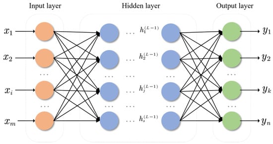
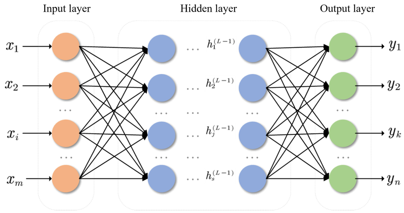
The Back Propagation Neural Network (BPNN) is an artificial neural network algorithm that performs supervised learning using gradient descent and the chain rule, proposed by Rumelhart et al. in 1986 [27]. It consists of the input layer, the hidden layer, and the output layer. It iteratively updates weights through error backpropagation until convergence is realized. It has demonstrated strong nonlinear fitting capabilities in crop water inversion and agricultural remote sensing modeling [28,29]. Considering the relatively limited sample size in this study, a relatively simple BPNN structure was adopted to reduce model complexity and mitigate the risk of overfitting. A single hidden layer containing 6 neurons was used for all irrigation treatments as a compromise between nonlinear fitting ability and model simplicity. This relatively small hidden-layer size was intended to avoid excessive model complexity under the current dataset and to maintain comparability across FD, ND, and MD by using a unified network structure. The activation function was set to tanh, and the network was optimized using the Adam optimizer with an initial learning rate of 0.001. The L2 regularization parameter (alpha) was set to 0.001, and the maximum number of iterations was set to 5000. Early stopping was enabled with a validation fraction of 0.15, and training was terminated when the validation performance did not improve for 30 consecutive iterations. The random seed was fixed at 42. Before model training, both input variables and target values were normalized to the range [−1, 1]. Potential overfitting was further evaluated by comparing the training and testing results in the predicted-versus-observed plots together with the corresponding residual boxplots. Its workflow is illustrated in Figure 2.
Figure 2.
Workflow of the BPNN model. Arrows indicate the direction of information flow, and different colors represent neurons in the input, hidden, and output layers. Ellipses indicate omitted neurons/layers for simplicity.
2.4.4. Model Evaluation Metrics
Model performance was evaluated using the coefficient of determination (R2), root mean squared error (RMSE), mean absolute error (MAE), and bias. Under the five-fold cross-validation framework, R2, RMSE, MAE, and bias were calculated from the testing subset in each fold, and the mean and standard deviation of these metrics across the five folds were used to assess model robustness. R2 reflects the proportion of variance explained by the model, while RMSE quantifies the magnitude of estimation errors. This framework is widely used in agricultural remote sensing studies [30,31]. R2, RMSE, MAE and bias were calculated as:
where yi represents the observed value, signifies the predicted value, denotes the mean of the observed values, and n means the number of samples.
2.5. Data Analysis
Correlation analysis and plotting were performed using Origin 2024. Data processing was conducted in Microsoft Excel 2013, while mosaicking of UAV multispectral images was performed using Pix4Dmapper (version 4.3.27). Vegetation index calculation was conducted using QGIS 3.30.2. Model simulation and analysis were implemented using Python 3.11.
3. Results and Analysis
3.1. Correlation Analysis Between Leaf Water Content and Phenotypic Factors Under Different Irrigation Methods
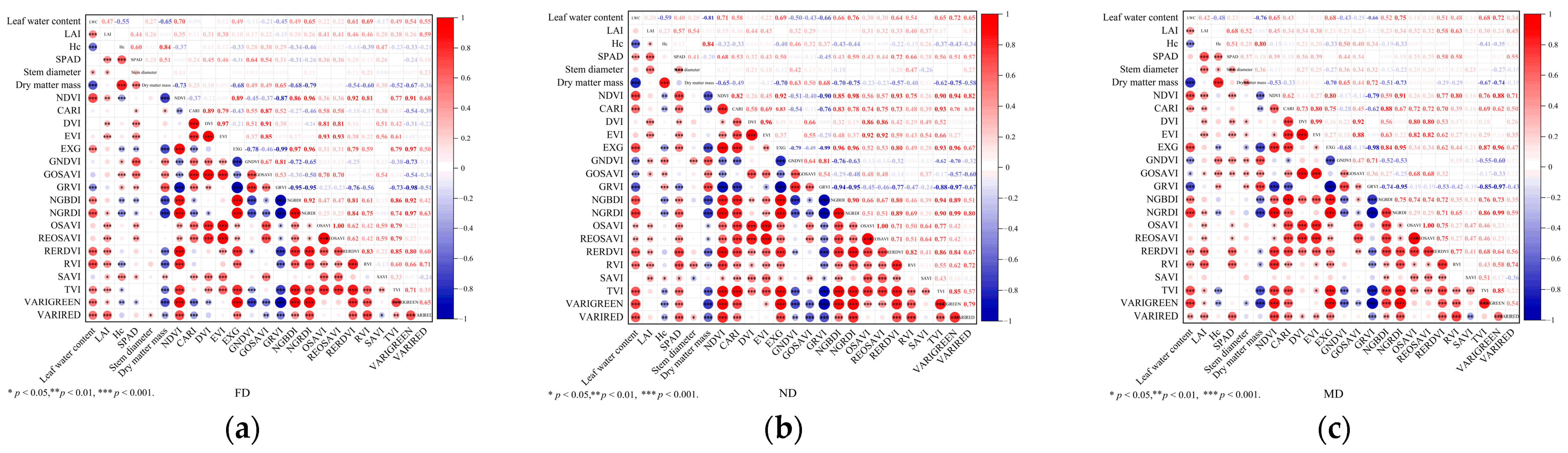
Based on data collected during 2023–2024, Pearson correlation analysis was conducted to examine the relationships between leaf water content and morphological traits as well as vegetation indices under different irrigation methods (Figure 3). Overall, LWC showed significant positive correlations with several vegetation indices under all three irrigation methods, whereas HC, DM, and GRVI generally showed negative relationships with LWC. However, the dominant sensitive indicators differed among irrigation treatments. Under FD, NDVI (r = 0.70), RVI (r = 0.69), NGRDI (r = 0.65), and RERDVI (r = 0.61) showed relatively strong correlations with LWC, indicating the greater sensitivity of ratio-based and red-edge-related indices. Under ND, NGRDI (r = 0.76), VARIGREEN (r = 0.72), and NDVI (r = 0.71) were the most strongly correlated indices, while DM showed the strongest negative correlation (r = −0.81). Under MD, NGRDI (r = 0.75) and VARIGREEN (r = 0.72) remained the most stable and highly correlated indicators, followed by TVI (r = 0.68) and NDVI (r = 0.65). Accordingly, NDVI, NGRDI, RERDVI, and RVI were selected as potential water-sensitive spectral indicators under FD; NDVI, NGRDI, VARIGREEN, EXG, NGBDI, RERDVI, TVI, and VARIRED under ND; and NGRDI, VARIGREEN, NDVI, EXG, TVI and GRVI under MD. Overall, the response relationships between LWC and spectral indices differed significantly among irrigation methods: FD was characterized by stronger sensitivity of red-edge and ratio-based indices, whereas ND and MD showed greater sensitivity of green-band-related indices, with NGRDI and VARIGREEN performing more stably under MD.
Figure 3.
Correlation analysis of leaf water content under FD, ND, and MD. (a) FD, film-mulched drip irrigation; (b) ND, non-mulched drip irrigation; and (c) MD, non-mulched shallow-buried drip irrigation. Asterisks indicate statistical significance levels: * p < 0.05, ** p < 0.01, *** p < 0.001.
3.2. Construction of Machine Learning-Based Models for Leaf Water Content (LWC) Estimation in Spring Wheat
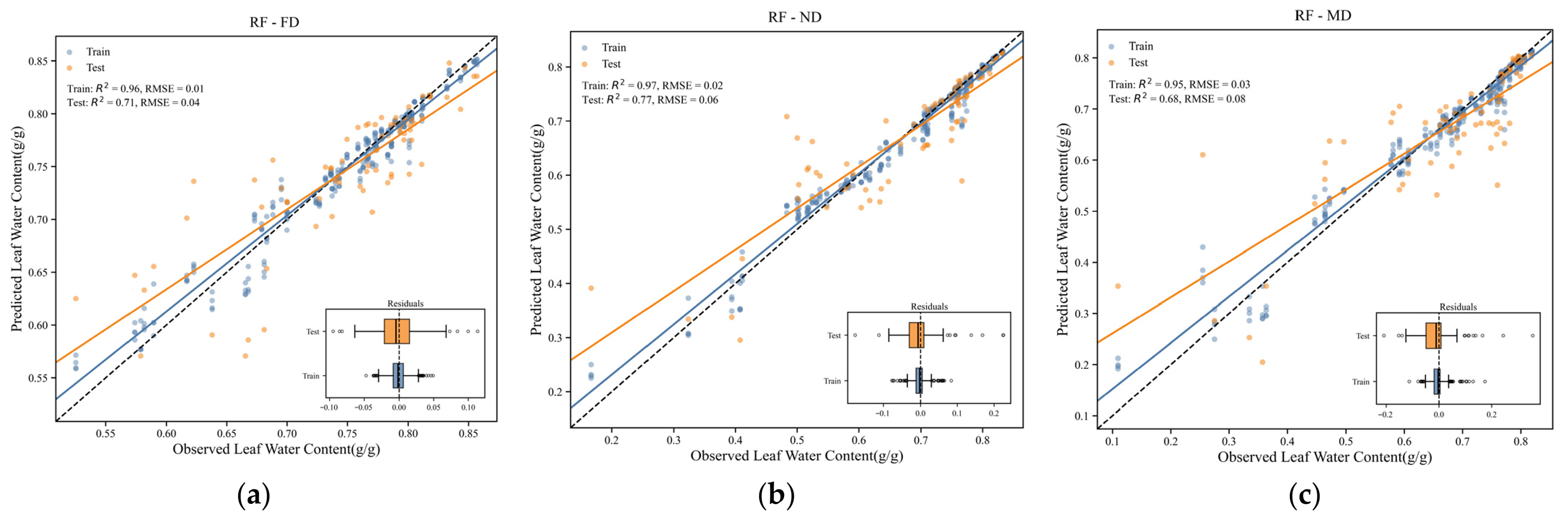
Based on the identified potential water-sensitive spectral indicators, Random Forest (RF) models were constructed for FD, ND, and MD. UAV multispectral vegetation indices and growth-related physiological indicators collected during 2023–2024 were used as input variables. The cross-validation results in terms of R2, RMSE, MAE, and bias are summarized in Table 4, and the comparisons between predicted and observed LWC values together with the corresponding residual boxplots are shown in Figure 4. Overall, the RF model showed relatively stable performance across the three irrigation treatments, with the best mean R2 observed under ND.
Table 4.
Mean ± SD of R2, RMSE, MAE, and bias for the RF model under FD, ND, and MD irrigation treatments based on five-fold cross-validation.
Figure 4.
Comparison of predicted and observed leaf water content using the RF model under (a) FD, (b) ND, and (c) MD irrigation treatments. The dashed line represents the 1:1 line between observed and predicted values.
Multiple linear regression (MLR) models were developed for FD, ND, and MD based on the selected water-sensitive spectral indicators. The model performance evaluated by five-fold cross-validation in terms of R2, RMSE, MAE, and bias is presented in Table 5.
Table 5.
Mean ± SD of R2, RMSE, MAE, and bias for the MLR model under FD, ND, and MD irrigation treatments based on five-fold cross-validation.
Under FD, the regression equation was as follows:
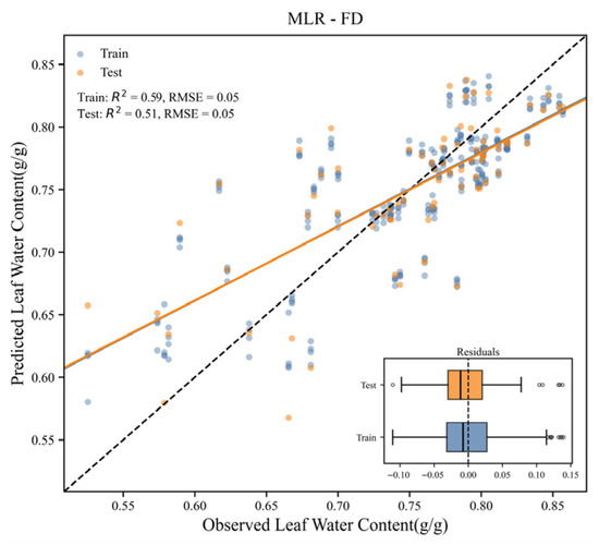
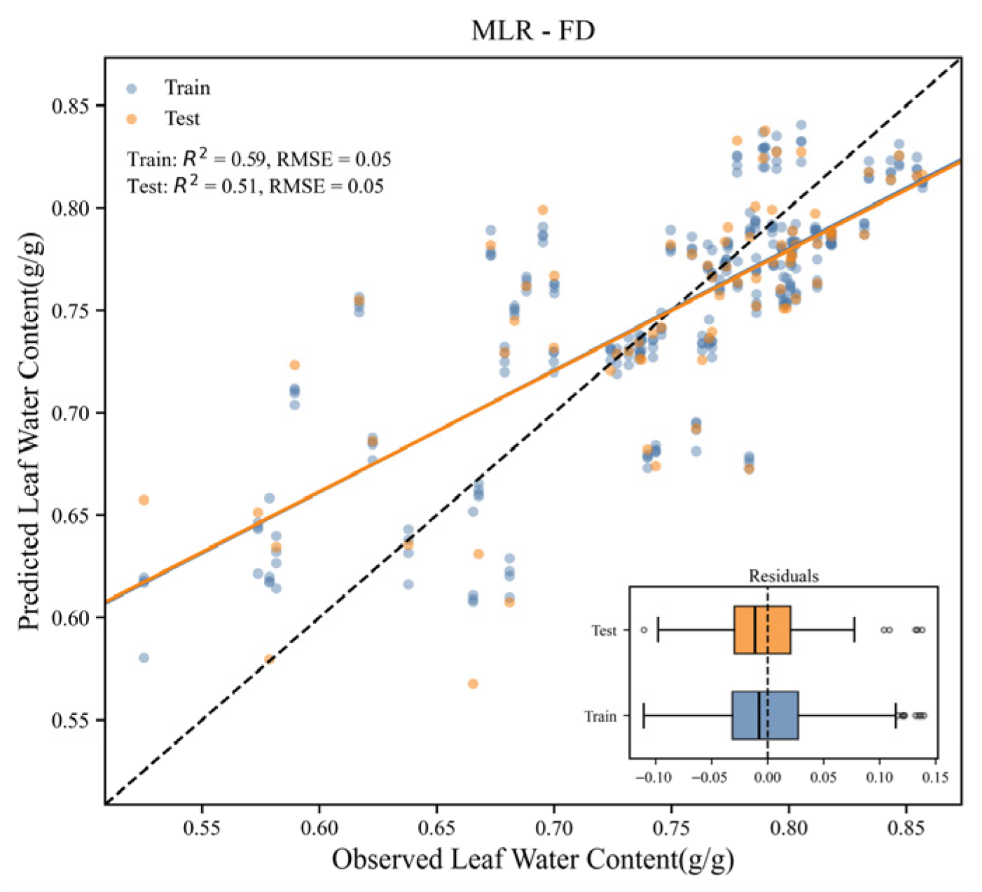
where Y represents the LWC, X1 − X4 signifies standardized NDVI, NGRDI, RERDVI, and RVI under FD, respectively. Figure 5 shows the comparison between the predicted and observed leaf water content (LWC) values, together with the residual boxplot, for the MLR model under FD irrigation treatment.
Y = 0.751 + 0.113X1 − 0.043X2 − 0.053X3 + 0.035X4
Figure 5.
Comparison of predicted and observed leaf water content using the MLR model under FD irrigation treatment. The dashed line represents the 1:1 line between observed and predicted values.
Under ND, the regression equation was as follows:
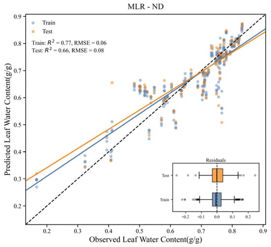
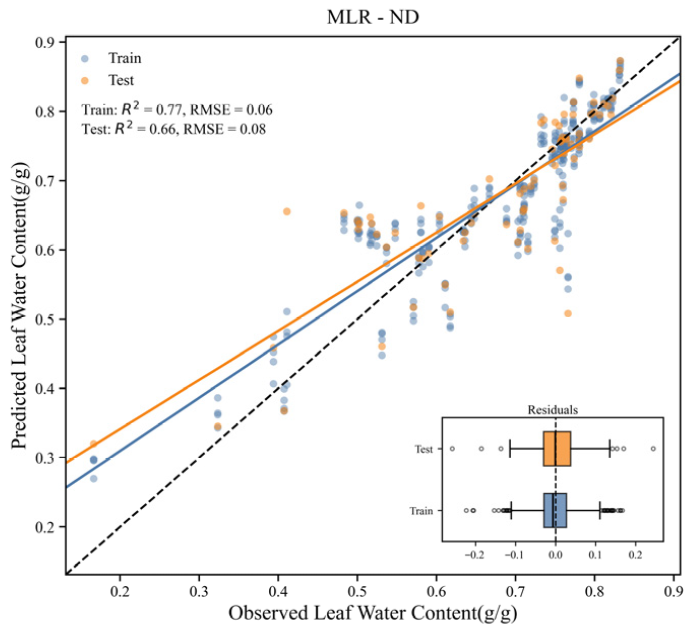
where Y is LWC, and X1 − X8 represents standardized NDVI, NGRDI, VARIGREEN, EXG, NGBDI, RERDVI, TVI, and VARIRED, respectively. Figure 6 shows the comparison between the predicted and observed leaf water content values, together with the residual boxplot, for the MLR model under ND irrigation treatment.
Y = 0.675 − 0.425X1 + 0.93X2 − 0.520X3 + 0.135X4 − 0.079X5 + 0.026213X6 − 0.027X7 + 0.050X8
Figure 6.
Comparison of predicted and observed leaf water content using the MLR model under ND irrigation treatment. The dashed line represents the 1:1 line between observed and predicted values.
Under MD, the regression equation was as follows:
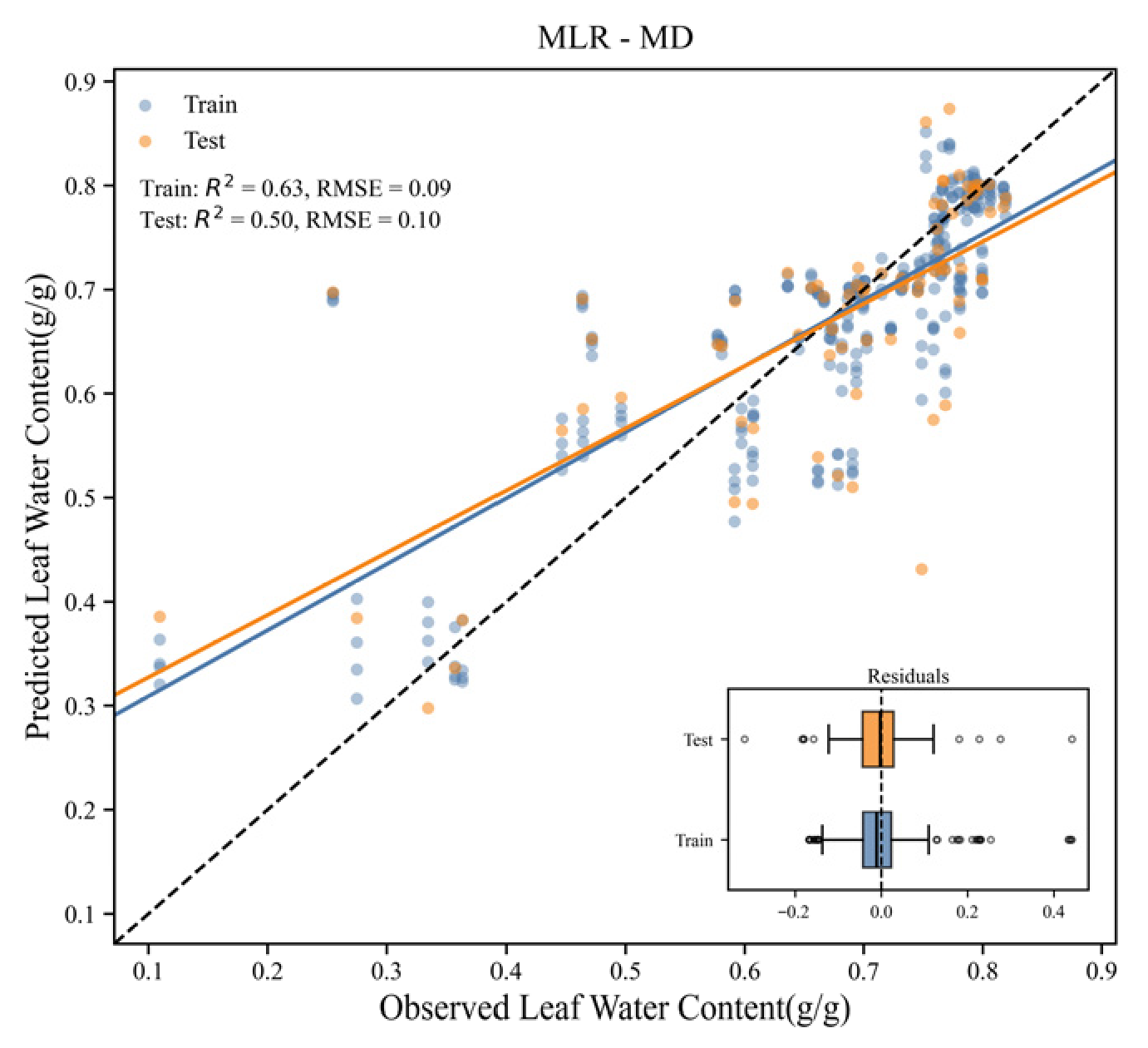
where Y is LWC, and X1 − X6 represents standardized NGRDI, VARIGREEN, NDVI, EXG, TVI, and GRVI, respectively. Figure 7 shows the comparison between the predicted and observed leaf water content values, together with the residual boxplot, for the MLR model under MD irrigation treatment.
Y = 0.672 + 0.245X1 + 0.039X2 − 0.073X3 − 0.037X4 + 0.044X5 + 0.114X6
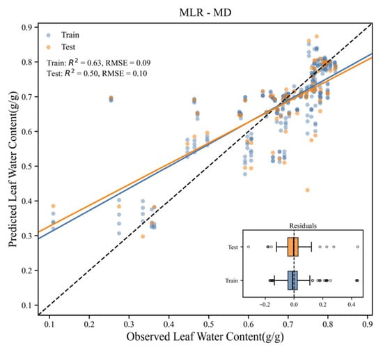
Figure 7.
Comparison of predicted and observed leaf water content using the MLR model under MD irrigation treatment. The dashed line represents the 1:1 line between observed and predicted values.
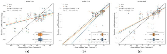
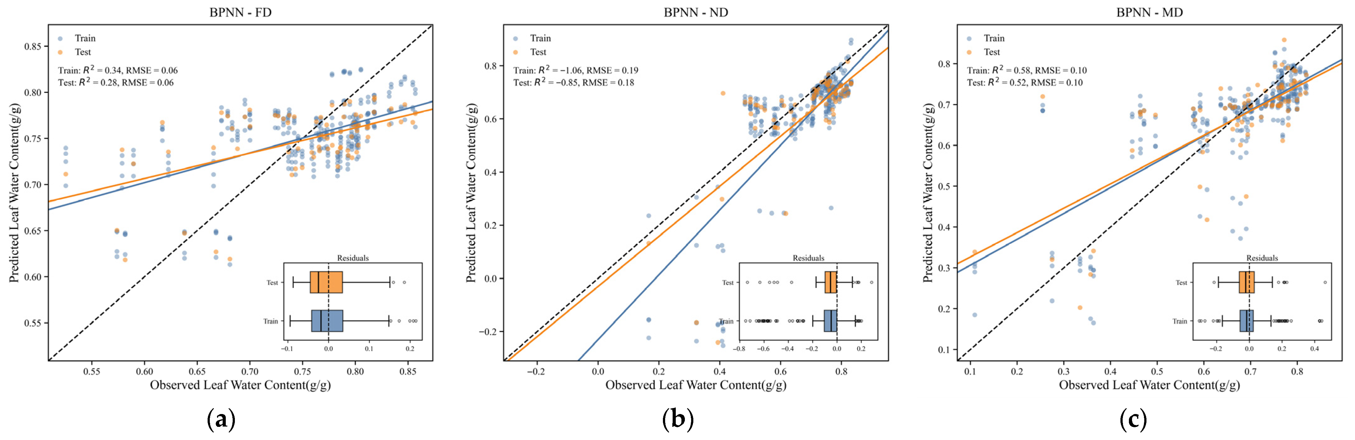
BPNN models were constructed for FD, ND, and MD based on the selected water-sensitive spectral indicators. Specifically, four indices (NDVI, NGRDI, RERDVI, and RVI) were used under FD, eight indices (NDVI, NGRDI, VARIGREEN, EXG, NGBDI, RERDVI, TVI, and VARIRED) under ND, and six indices (NGRDI, VARIGREEN, NDVI, EXG, TVI, and GRVI) under MD, with LWC as the output variable. In all three irrigation treatments, the BPNN model adopted a single hidden layer with 6 neurons. To improve the robustness of model evaluation under the relatively limited sample size, a five-fold cross-validation framework was adopted. Within each fold, an internal validation subset was further split from the training data for early stopping and model stabilization. Figure 8 presents the comparison between the predicted and observed leaf water content values obtained by the BPNN model under (a) FD, (b) ND, and (c) MD irrigation treatments, together with the corresponding residual boxplots, while the cross-validation results in terms of R2, RMSE, MAE, and bias are summarized in Table 6.
Figure 8.
Comparison of predicted and observed leaf water content using the BPNN model under (a) FD, (b) ND, and (c) MD irrigation treatments.
Table 6.
Mean ± SD of R2, RMSE, MAE, and bias for the BPNN model under FD, ND, and MD irrigation treatments based on five-fold cross-validation.
Among the three irrigation treatments, the BPNN model showed relatively better mean performance under MD, whereas it performed poorly and unstably under ND.
4. Discussion
4.1. Irrigation-Dependent Spectral Responses and LWC Estimation
This study demonstrated that the response relationships between LWC and spectral indices varied significantly among irrigation methods. Under FD, ratio-based and red-edge-related indices (e.g., NDVI, NGRDI, RERDVI, and RVI) exhibited stronger correlations with LWC. Under ND, indices reflecting canopy greenness (VARIGREEN and EXG) showed enhanced sensitivity to LWC. Under MD, NGRDI and VARIGREEN exhibited relatively stable relationships with LWC. These findings suggest that different irrigation management practices may alter soil–plant water supply dynamics and canopy structural characteristics, thereby influencing canopy spectral reflectance and water-response mechanisms. From a physiological perspective, different irrigation methods may have altered the timing, intensity, and spatial distribution of root-zone water supply, thereby influencing leaf water status, chlorophyll dynamics, canopy expansion, and senescence. Under FD, film mulching may have reduced soil evaporation and maintained a relatively more stable hydrothermal environment, which may have favored fuller canopy development and reduced exposed soil background, thereby enhancing the sensitivity of ratio-based and red-edge-related indices such as NDVI, RERDVI, and RVI to LWC. Under ND, stronger direct soil evaporation and a more exposed canopy–soil background may have made visible green-band-related indices such as VARIGREEN and EXG more responsive to changes in leaf greenness, pigment status, and partial canopy senescence. Under MD, shallow-buried drip irrigation may have changed the spatial wetting pattern of the root zone and buffered surface evaporation, resulting in relatively stable but still water-sensitive responses in indices such as NGRDI and VARIGREEN. From a radiative transfer perspective, these irrigation-induced differences may have affected both canopy structure and the contribution of soil background reflectance to the measured signal, thereby modifying the spectral sensitivity of different vegetation indices to LWC. In UAV-based multispectral remote sensing studies on wheat water status assessment, vegetation indices are widely regarded as key indicators of water stress, as they capture variations in canopy coverage and spectral reflectance associated with crop water conditions. This has been validated by multiple crop water monitoring studies [32,33,34].
Regarding model comparison, different machine learning algorithms exhibited irrigation-dependent performance differences. In this study, the Random Forest (RF) model achieved higher estimation accuracy under FD and MD. This may be related to its strong capability in modeling nonlinear relationships and complex interactions among input variables. Previous studies have similarly reported that RF often provides higher stability and predictive accuracy in UAV-based multispectral inversion of soil and crop water parameters [35]. In contrast, the BPNN model did not show stable predictive performance across irrigation treatments, particularly under ND, where large fold-to-fold variability and negative mean R2 values were observed. This suggests that BPNN may have been sensitive to data partitioning under the current sample size and model configuration. The multiple linear regression (MLR) model showed lower accuracy across irrigation methods, indicating that a purely linear formulation may be insufficient to capture the relationship between LWC and multispectral indices. This observation is consistent with recent findings in UAV-based remote sensing studies for water-related trait prediction, where nonlinear machine learning models generally outperform linear methods [36]. However, these interpretations are based mainly on general model characteristics and observed prediction behavior, because deeper analyses of model behavior, feature interactions, and variable contributions were not explicitly performed in this study. Therefore, the above explanations should be regarded as plausible interpretations rather than definitive conclusions.
Quantitatively, the accuracy of the present RF models under the three irrigation treatments (mean R2 = 0.62−0.74; mean RMSE = 0.04−0.08) was broadly comparable to the performance range reported in recent UAV-based wheat water-status studies using single-source multispectral features. For instance, Yu et al. [7] reported that winter wheat LWC estimation based only on multispectral features achieved R2 values of 0.526−0.718, whereas multispectral–texture fusion improved R2 to 0.748−0.815 and a stacking ensemble model further increased R2 to 0.865. Likewise, Zhao et al. [32] reported test-set R2 values of 0.69−0.87 and RMSE values of 0.04−0.08 for UAV-based winter wheat water-stress estimation using multifeature fusion and stacking ensemble learning. These comparisons suggest that the present irrigation-specific RF models achieved reasonable accuracy using a relatively simple multispectral-feature framework, although their performance remained lower than that of more advanced feature-fusion and ensemble-based approaches. Recent studies further support this interpretation. For example, Mali et al. [11] reported that combining UAV-based multispectral and thermal infrared imagery with machine learning improved winter wheat water-stress prediction under field conditions, highlighting the value of multi-sensor information for enhancing model robustness. Similarly, Yang et al. [10] showed that model updating strategies can improve crop water status evaluation from UAV imagery under varying field conditions, indicating that temporal adaptation is also important for stable prediction. Compared with these studies, the present work focused on irrigation-specific LWC estimation using only multispectral features and still achieved reasonable performance, suggesting that irrigation-specific modeling itself can provide useful improvements even within a relatively simple data framework.
Overall, integrating UAV multispectral data with machine learning algorithms can improve LWC estimation accuracy under different irrigation methods. Model performance was strongly influenced by irrigation management, highlighting the importance of irrigation-specific modeling strategies. These findings provide empirical support for understanding irrigation-dependent spectral–water response patterns under the present experimental conditions and offer preliminary practical insight for crop water-status diagnosis and irrigation-management support. From a practical perspective, the developed irrigation-specific models may be useful for plot-scale monitoring of spring wheat water status and for supporting irrigation decision-making in arid agricultural regions, particularly when rapid and non-destructive assessment is needed. However, their field applicability at broader operational scales still requires further validation under multi-site, multi-year, and more heterogeneous management conditions.
4.2. Limitations and Future Perspectives
Although this study confirmed the feasibility of using UAV-based multispectral imagery for LWC estimation in spring wheat under arid conditions, several limitations should be acknowledged. The models were developed based on plot-scale experiments conducted at a single location over two growing seasons. Therefore, their generalization and external applicability across broader arid regions remain limited, and explicit external validation using independent datasets from different sites, years, and management conditions is needed before broader application. In addition, temporal effects, including growth-stage variability and interannual differences between the 2023 and 2024 seasons, were not explicitly assessed. As a result, the reported model accuracies represent pooled predictive performance rather than formal temporal validation. Future work should include stage-specific analysis and inter-annual transferability tests to better evaluate temporal robustness.
First, the multispectral dataset contained only five bands (red, green, blue, near-infrared, and red-edge), which may restrict the spectral sensitivity to water-related absorption features. Recent studies have concluded that leaf water status is particularly sensitive to absorption features near 970 nm, and incorporating higher spectral resolution data (e.g., hyperspectral imagery) can improve the accuracy of water stress detection and inversion [37,38]. Furthermore, recent reviews on UAV-based water monitoring highlight that multi-sensor integration (e.g., hyperspectral and thermal infrared sensors) and feature-level data fusion are critical directions for enhancing robustness in water information extraction [36]. Therefore, future research should integrate hyperspectral data or multi-source sensor fusion to capture richer water-sensitive spectral information and enhance model generalization.
Second, the irrigation gradient design may fail to fully represent a broader range of water stress scenarios. In addition, crop water stress was regulated through soil-moisture-based irrigation thresholds, while independent physiological stress indicators were not simultaneously measured. Future studies should combine soil moisture regulation with physiological stress diagnostics to improve the agronomic interpretation of irrigation treatments. Limited variability under extremely deficit or sufficient irrigation conditions may constrain the extrapolation capability of the models. Future studies should expand irrigation gradients and experimental scales, and incorporate multi-year and multi-site datasets to increase sample heterogeneity and improve model robustness.
Third, sensitive variable selection in this study was primarily based on Pearson correlation analysis. Although this method is effective for preliminary dimensionality reduction and for identifying irrigation-specific candidate indicators, it remains a linear and pairwise screening approach that does not fully capture nonlinear relationships or interactions among predictors. In addition, multicollinearity among the selected vegetation indices was not explicitly assessed using dedicated statistical diagnostics, and some redundancy may still exist because several indices were derived from overlapping spectral bands. In recent years, explainable artificial intelligence (XAI) methods have gained increasing attention in agricultural remote sensing. Techniques such as SHAP and permutation importance can provide transparent interpretation of model decisions and quantify the relative contributions of spectral bands or indices to water status estimation, thereby improving model interpretability and credibility [39]. Future studies should incorporate variance inflation factor (VIF) analysis, recursive feature elimination (RFE), variable importance ranking, or SHAP-based interpretation to refine feature selection and enhance model transparency.
Finally, the relatively limited sample size may have constrained the full potential of certain machine learning models, as the final dataset used for model construction consisted of 75 treatment-level samples for each irrigation method and 225 samples in total across the three irrigation methods. In addition, uncertainty analysis and replication error propagation were not explicitly quantified in this study, which should be considered when interpreting the model results. Although five-fold cross-validation, internal validation, and early stopping were adopted to reduce overfitting risk, the robustness and generalization ability of the neural network model still require further verification using larger multi-year and multi-site datasets. Increasing the sample size and incorporating multi-year and multi-regional datasets would further enhance robustness and generalization capabilities of the models. Future studies should include explicit external validation using independent datasets to better assess model robustness and transferability under broader field conditions.
5. Conclusions
Based on two-year field experiments conducted in 2023–2024 in an arid region of Northwest China, this study developed irrigation-specific models for estimating spring wheat LWC from UAV multispectral imagery and compared the performance of MLR, RF, and BPNN models. The main conclusions are as follows:
- (1)
- Spectral indicators sensitive to LWC differed among irrigation methods. Red-edge and ratio-based indices were more sensitive under FD, whereas green-band-related indices showed stronger responses under ND and MD.
- (2)
- Model performance was irrigation-dependent. Among the tested models, RF showed the most stable overall performance across FD, ND, and MD, while BPNN exhibited limited robustness under the current dataset, particularly under ND.
- (3)
- Irrigation-specific modeling improved the characterization of spectral–water relationships and showed good potential for UAV-based LWC estimation in spring wheat under arid conditions.
Overall, the results highlight the importance of considering irrigation effects in UAV-based crop water status monitoring and provide useful support for irrigation management and precision agriculture, particularly for plot-scale water diagnosis and irrigation decision-making in spring wheat under arid conditions.
Author Contributions
Conceptualization, J.Z., P.Z. and H.C.; validation, H.C.; formal analysis, J.Z. and P.Z.; investigation, J.Z., P.Z., X.A. and N.L.; resources, S.L.; data curation, J.Z., P.Z., X.A., H.C. and N.L.; writing—original draft preparation, J.Z. and P.Z.; writing—review and editing, J.Z. and Y.Z.; visualization, J.Z. and P.Z.; supervision, S.L. and Y.Z.; project administration, S.L.; funding acquisition, S.L. S.L. served as the corresponding author. All authors have read and agreed to the published version of the manuscript.
Funding
This research was funded by the National Natural Science Foundation of China (52379052) and National Key Research and Development Program of China (2022YFD1900801).
Data Availability Statement
The original contributions presented in this study are included in the article. Further inquiries can be directed to the corresponding author.
Conflicts of Interest
The authors declare no conflicts of interest.
References
- Rasheed, M.W.; Tang, J.; Sarwar, A.; Shah, S.; Saddique, N.; Khan, M.U.; Imran Khan, M.; Nawaz, S.; Shamshiri, R.R.; Aziz, M.; et al. Soil Moisture Measuring Techniques and Factors Affecting the Moisture Dynamics: A Comprehensive Review. Sustainability 2022, 14, 11538. [Google Scholar] [CrossRef] [Scilit]
- Shawon, S.M.; Neha, N.I.; Jui, A.N.; Dey, N.; Zubair, H.T. Advances in Soil Moisture Measurement Techniques and Prediction using Artificial Intelligence: An Extensive and Systematic Review. Smart Agric. Technol. 2025, 12, 101613. [Google Scholar] [CrossRef] [Scilit]
- Xie, C.; Yang, C. A review on plant high-throughput phenotyping traits using UAV-based sensors. Comput. Electron. Agric. 2020, 178, 105731. [Google Scholar] [CrossRef] [Scilit]
- Feng, L.; Chen, S.; Zhang, C.; Zhang, Y.; He, Y. A comprehensive review on recent applications of unmanned aerial vehicle remote sensing with various sensors for high-throughput plant phenotyping. Comput. Electron. Agric. 2021, 182, 106033. [Google Scholar] [CrossRef] [Scilit]
- Gano, B.; Bhadra, S.; Vilbig, J.M.; Ahmed, N.; Sagan, V.; Shakoor, N. Drone-based imaging sensors, techniques, and applications in plant phenotyping for crop breeding: A comprehensive review. Plant Phenome J. 2024, 7, e20100. [Google Scholar] [CrossRef] [Scilit]
- Zhou, H.; Zhou, G.; Song, X.; He, Q. Dynamic Characteristics of Canopy and Vegetation Water Content during an Entire Maize Growing Season in Relation to Spectral-Based Indices. Remote Sens. 2022, 14, 584. [Google Scholar] [CrossRef] [Scilit]
- Yu, X.; Qian, L.; Chen, K.; Ye, S.; Yin, Q.; Shao, L.; Ran, D.; Wang, W.; Zhang, B.; Hu, X. Estimating Winter Wheat Leaf Water Content by Combining UAV Spectral and Texture Features with Stacking Ensemble Learning. Agronomy 2025, 15, 2610. [Google Scholar] [CrossRef] [Scilit]
- Holman, F.H.; Riche, A.B.; Michalski, A.; Castle, M.; Wooster, M.J.; Hawkesford, M.J. High Throughput Field Phenotyping of Wheat Plant Height and Growth Rate in Field Plot Trials Using UAV Based Remote Sensing. Remote Sens. 2016, 8, 1031. [Google Scholar] [CrossRef] [Scilit]
- Ma, S.; Liu, S.; Gao, Z.; Wang, X.; Ma, S.; Wang, S. Water Deficit Diagnosis of Winter Wheat Based on Thermal Infrared Imaging. Plants 2024, 13, 361. [Google Scholar] [CrossRef] [Scilit] [PubMed]
- Yang, N.; Zhang, Z.; Yang, X.; Dong, N.; Xu, Q.; Chen, J.; Sun, S.; Cui, N.; Ning, J. Evaluation of crop water status using UAV-based images data with a model updating strategy. Agric. Water Manag. 2025, 312, 109445. [Google Scholar] [CrossRef] [Scilit]
- Mali, S.S.; Scobie, M.; Baillie, J.; Plant, C.; Shammi, S.; Das, A. Integrating UAV-based multispectral and thermal infrared imageries with machine learning for predicting water stress in winter wheat. Precis. Agric. 2025, 26, 44. [Google Scholar] [CrossRef] [Scilit]
- Ramírez-Cuesta, J.M.; Martínez-Gimeno, M.A.; Badal, E.; Tasa, M.; Bonet, L.; Pérez-Pérez, J.G. UAV-based multispectral and thermal indexes for estimating crop water status and yield on super-high-density olive orchards under deficit irrigation conditions. Precis. Agric. 2025, 26, 47. [Google Scholar] [CrossRef] [Scilit]
- Yacoob, A.; Gokool, S.; Clulow, A.; Mahomed, M.; Naiken, V.; Mabhaudhi, T. A machine learning approach for quantifying crop water stress in smallholder farms using unmanned aerial vehicle multispectral imagery. Agric. Water Manag. 2026, 324, 110142. [Google Scholar] [CrossRef] [Scilit]
- Yaseen, M.U.; Saddique, G.; Ashraf, M.; Yasmeen, Z.; Ahmad, S. Design, development and testing of mobile sprinkler raingun for smart irrigation in arid zone-based crops. J. Agric. Res. 2019, 57, 103–112. [Google Scholar]
- Rouse, J.W., Jr.; Haas, R.H.; Deering, D.W.; Schell, J.A.; Harlan, J.C. Monitoring the Vernal Advancement and Retrogradation (Green Wave Effect) of Natural Vegetation; (No. E75-10354); NASA: Washington, DC, USA, 1974.
- Huete, A.R. A soil-adjusted vegetation index (SAVI). Remote Sens. Environ. 1988, 25, 295–309. [Google Scholar] [CrossRef] [Scilit]
- Pearson, R.L.; Miller, L.D. Remote mapping of standing crop biomass for estimation of the productivity of the shortgrass prairie, Pawnee National Grasslands, Colorado. In Proceedings of the Eighth International Symposium on Remote Sensing of Environment, Ann Arbor, MI, USA, 2–6 October 1972. [Google Scholar]
- Broge, N.H.; Leblanc, E. Comparing prediction power and stability of broadband and hyperspectral vegetation indices for estimation of green leaf area index and canopy chlorophyll density. Remote Sens. Environ. 2001, 76, 156–172. [Google Scholar] [CrossRef] [Scilit]
- Torres-Sánchez, J.; Pena, J.M.; de Castro, A.I.; López-Granados, F. Multi-temporal mapping of the vegetation fraction in early-season wheat fields using images from UAV. Comput. Electron. Agric. 2014, 103, 104–113. [Google Scholar] [CrossRef] [Scilit]
- Hunt, E.R., Jr.; Cavigelli, M.; Daughtry, C.S.; Mcmurtrey, J.E., III; Walthall, C.L. Evaluation of digital photography from model aircraft for remote sensing of crop biomass and nitrogen status. Precis. Agric. 2005, 6, 359–378. [Google Scholar] [CrossRef] [Scilit]
- Kim, M.S.; Daughtry, C.S.T.; Chappelle, E.W.; McMurtrey, J.E.; Walthall, C.L. The use of high spectral resolution bands for estimating absorbed photosynthetically active radiation (A par). In Proceedings of 6th International Symposium on Physical Measurements and Signatures in Remote Sensing; No. GSFC-E-DAA-TN72921; CNES: Paris Cedex, France, 1994. [Google Scholar]
- Montgomery, D.C.; Peck, E.A.; Vining, G.G. Introduction to Linear Regression Analysis; John Wiley & Sons: Hoboken, NJ, USA, 2012. [Google Scholar]
- Dormann, C.F.; Elith, J.; Bacher, S.; Buchmann, C.; Carl, G.; Carré, G.; Marquéz, J.R.G.; Gruber, B.; Lafourcade, B.; Leitão, P.J.; et al. Collinearity: A review of methods to deal with it and a simulation study evaluating their performance. Ecography 2013, 36, 27–46. [Google Scholar] [CrossRef] [Scilit]
- Breiman, L. Random forests. Mach. Learn. 2001, 45, 5–32. [Google Scholar] [CrossRef] [Scilit]
- Belgiu, M.; Drăguţ, L. Random forest in remote sensing: A review of applications and future directions. ISPRS J. Photogramm. Remote Sens. 2016, 114, 24–31. [Google Scholar] [CrossRef] [Scilit]
- Jeong, J.H.; Resop, J.P.; Mueller, N.D.; Fleisher, D.H.; Yun, K.; Butler, E.E.; Timlin, D.J.; Shim, K.M.; Gerber, J.S.; Reddy, V.R.; et al. Random forests for global and regional crop yield predictions. PLoS ONE 2016, 11, e0156571. [Google Scholar] [CrossRef] [Scilit] [PubMed]
- Rumelhart, D.E.; Hinton, G.E.; Williams, R.J. Learning representations by back-propagating errors. Nature 1986, 323, 533–536. [Google Scholar] [CrossRef] [Scilit]
- Liakos, K.G.; Busato, P.; Moshou, D.; Pearson, S.; Bochtis, D. Machine learning in agriculture: A review. Sensors 2018, 18, 2674. [Google Scholar] [CrossRef] [Scilit]
- Ma, L.; Liu, Y.; Zhang, X.; Ye, Y.; Yin, G.; Johnson, B.A. Deep learning in remote sensing applications: A meta-analysis and review. ISPRS J. Photogramm. Remote Sens. 2019, 152, 166–177. [Google Scholar] [CrossRef] [Scilit]
- Willmott, C.J.; Matsuura, K. Advantages of the mean absolute error (MAE) over the root mean square error (RMSE) in assessing average model performance. Clim. Res. 2005, 30, 79–82. [Google Scholar] [CrossRef] [Scilit]
- Chai, T.; Draxler, R.R. Root mean square error (RMSE) or mean absolute error (MAE)?–Arguments against avoiding RMSE in the literature. Geosci. Model Dev. 2014, 7, 1247–1250. [Google Scholar] [CrossRef] [Scilit]
- Zhao, H.; Wang, J.; Guo, J.; Hui, X.; Wang, Y.; Cai, D.; Yan, H. Detecting Water Stress in Winter Wheat Based on Multifeature Fusion from UAV Remote Sensing and Stacking Ensemble Learning Method. Remote Sens. 2024, 16, 4100. [Google Scholar] [CrossRef] [Scilit]
- Solgi, S.; Ahmadi, S.H.; Seidel, S.J. Remote sensing of canopy water status of the irrigated winter wheat fields and the paired anomaly analyses on the spectral vegetation indices and grain yields. Agric. Water Manag. 2023, 280, 108226. [Google Scholar] [CrossRef] [Scilit]
- Li, Z.; Cheng, Q.; Chen, Z.; Xiang, Y.; Hu, X.; Lazarovitch, N.; Zhen, J. Estimating soil water content of cotton fields using UAV-based multi-source remote sensing data fusion. Agric. Water Manag. 2025, 322, 109996. [Google Scholar] [CrossRef] [Scilit]
- Zhang, Z.; Dou, G.; Zhao, X.; Gao, Y.; Liu, S.; Qin, A. Inversion of Crop Water Content Using Multispectral Data and Machine Learning Algorithms in the North China Plain. Agronomy 2024, 14, 2361. [Google Scholar] [CrossRef] [Scilit]
- Dong, H.; Dong, J.; Sun, S.; Bai, T.; Zhao, D.; Yin, Y.; Shen, X.; Wang, Y.; Zhang, Z.; Wang, Y. Crop water stress detection based on UAV remote sensing systems. Agric. Water Manag. 2024, 303, 109059. [Google Scholar] [CrossRef] [Scilit]
- Matese, A.; Prince Czarnecki, J.M.; Samiappan, S.; Moorhead, R. Are unmanned aerial vehicle-based hyperspectral imaging and machine learning advancing crop science? Trends Plant Sci. 2024, 29, 196–209. [Google Scholar] [CrossRef] [Scilit] [PubMed]
- Špundová, M.; Kučerová, Z.; Nožková, V.; Opatíková, M.; Procházková, L.; Klimeš, P.; Nauš, J. What to Choose for Estimating Leaf Water Status—Spectral Reflectance or In vivo Chlorophyll Fluorescence? Plant Phenom. 2024, 6, 0243. [Google Scholar] [CrossRef] [Scilit]
- Shi, B.; Chen, X.; Guo, Y.; Liu, L.; Li, P.; Chang, Q. Multi-Source Feature Selection and Explainable Machine Learning Approach for Mapping Nitrogen Balance Index in Winter Wheat Based on Sentinel-2 Data. Remote Sens. 2025, 17, 3196. [Google Scholar] [CrossRef] [Scilit]

Disclaimer/Publisher’s Note: The statements, opinions and data contained in all publications are solely those of the individual author(s) and contributor(s) and not of MDPI and/or the editor(s). MDPI and/or the editor(s) disclaim responsibility for any injury to people or property resulting from any ideas, methods, instructions or products referred to in the content. |
© 2026 by the authors. Licensee MDPI, Basel, Switzerland. This article is an open access article distributed under the terms and conditions of the Creative Commons Attribution (CC BY) license.