Mapping Surface-Cover Components in Desert Steppe from UAV RGB Imagery Using Interpretable Features and Multiscale Superpixel Probability Fusion

Abstract

Unmanned aerial vehicle (UAV) red–green–blue (RGB) imagery provides low-cost, high-resolution observations of desert-steppe cover, but overlapping colors and spatial heterogeneity complicate classification. We evaluated random forest (RF) with multiscale superpixel probability fusion (RF-MSPF) using 19 patches from nine images and 335,675 reference pixels representing herbaceous vegetation, woody or semi-woody vegetation, visible dead plant material, and bare substrate. Five interpretable RGB features supplied RF class probabilities, aggregated within Simple Linear Iterative Clustering (SLIC) regions at three scales. Source-image-grouped five-fold validation increased mean overall accuracy (OA) from 0.8020 ± 0.0573 for RF to 0.8691 ± 0.0367 for RF-MSPF (mean ± sample standard deviation), with gains in every fold. Equal-weight fusion achieved 0.8704 ± 0.0367. On the fixed development split, RF-MSPF achieved OA = 0.8806, macro-averaged F1 (Macro-F1) = 0.8742, and mean intersection over union (mIoU) = 0.7840. Ablations identified regional aggregation as the main improvement, with further gains from multiscale fusion; consistency weighting added only 0.024 percentage points on that split and showed no consistent advantage. This transparent, reproducible workflow improved classification within this dataset.

1. Introduction

Desert steppe is an important ecosystem in arid and semiarid regions. Its surface commonly comprises perennial herbs, woody or semi-woody plants, dead plant material, and bare substrate arranged in heterogeneous patch mosaics. High-resolution unmanned aerial vehicle (UAV) observations complement field surveys and medium- to coarse-resolution satellite observations in grassland monitoring [1]. Distinguishing herbaceous cover, woody or semi-woody canopies, dead plant material, and exposed surfaces provides information on surface composition and spatial heterogeneity beyond a single measure of green vegetation cover [2]. Grassland shrub mapping and combined UAV–satellite studies also demonstrate the relevance of separating herbaceous and woody cover for characterizing surface structure and extending analyses across spatial scales [3,4]. Low-cost mapping of these components can therefore support desert-steppe surveys and repeated monitoring.

Consumer-grade UAV red–green–blue (RGB) cameras offer low acquisition costs, flexible operation, and fine spatial detail. Moreno et al. investigated forage-crop segmentation in RGB imagery [5]. Pranga et al. combined RGB and multispectral UAV imagery to quantify grass–clover species composition [6], while Hu et al. estimated vegetation fractional cover using smartphones [7]. A review of UAV grassland biomass estimation also highlights color, texture, and spatial information [8]. Sparse desert-steppe cover nevertheless presents specific classification difficulties. Herbaceous vegetation (HV) and woody or semi-woody vegetation (WV) can both contain green tissues. Visible dead plant material (LT) and bare substrate (BS), including pale soil or gravel, can share yellow–brown colors. Branches, leaves, shadows, and exposed substrate also intermix at fine spatial scales, creating local variation in pixel features and potentially fragmented pixelwise predictions.

RGB vegetation indices, color-space transformations, and texture features describe complementary aspects of visible imagery. Previous studies have used RGB bands, vegetation indices, and texture to identify grassland and other vegetation cover [9,10], while highlighting the effects of illumination, color representation, and texture on vegetation extraction [11,12]. Random forest (RF), nearest-neighbor, and gradient-boosting methods can use such engineered features for classification or regression [13,14]. Object- and region-based approaches add neighborhood and morphological information and have been applied to seminatural grassland and woody vegetation mapping [15,16]. For UAV RGB datasets with few source images and sparse regional labels, low-dimensional features with explicit mathematical meanings and a probabilistic classifier provide a transparent basis for examining the contributions of input information and spatial processing.

Simple Linear Iterative Clustering (SLIC) groups spatially adjacent pixels with similar appearances into local regions, linking pixel predictions to spatial structure [17]. Studies of hyperspectral imagery using multiscale superpixels and hierarchical homogeneous regions suggest that different region sizes can provide complementary spatial representations [18,19]. Recent UAV grassland research has also placed greater emphasis on separating green vegetation, dead material, and bare surfaces [20,21]. A more specific question remains for low-cost UAV RGB mapping in desert steppe: with the pixel classifier and its probability outputs held constant, how much improvement comes from regional probability aggregation, multiscale integration, and consistency weighting, respectively? Comparing these steps separately helps identify the spatial operation responsible for the final performance.

We developed a workflow combining random forest with multiscale superpixel probability fusion (RF-MSPF) for mapping four RGB-visible surface-cover components in desert steppe, focusing on the roles of input features and spatial processing. The objectives were to (1) construct five interpretable features describing color, hue, regional edges, and directional texture; (2) compare single-scale regional aggregation, multiscale equal-weight fusion, and consistency weighting using the same RF probabilities; and (3) evaluate classification across source-image groups within the study site using grouped five-fold validation, alongside class-specific errors, feature combinations, and computational cost.

2. Materials and Methods

2.1. Study Area, UAV Data, and Reference Labeling

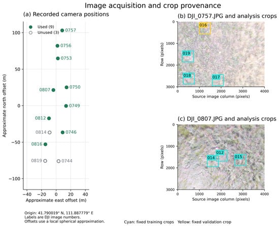
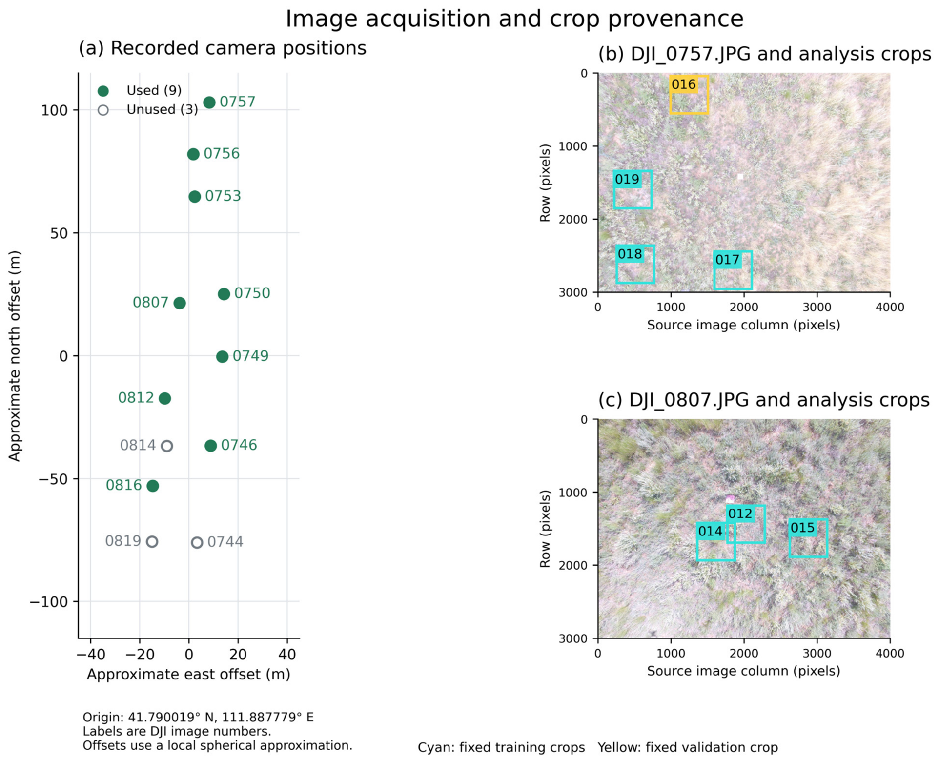
The study was conducted in desert steppe near Gegentala, Siziwang Banner, Inner Mongolia, China, where source-image GPS records cluster near 41.7900° N, 111.8878° E. Figure 1 shows recorded camera positions and example analysis crops; the camera positions do not delineate surveyed ground boundaries. The landscape comprises sparse plant cover interspersed with exposed substrate. Previous studies in Siziwang Banner describe desert-steppe vegetation including Stipa breviflora, Cleistogenes songorica, and Artemisia frigida [22,23], providing regional ecological context for this study.

Figure 1. Source-image positions and crop provenance. (a) Recorded GPS camera positions: filled symbols identify the nine analyzed sources and open symbols the three other retained images. Positions do not delineate a surveyed boundary. (b,c) Sources DJI_0757.JPG and DJI_0807.JPG with 512 × 512 training (cyan) and validation (yellow) crops. Axes are source-image pixels; patch identifiers correspond to Table S3a.

Images were acquired on 4–5 July 2025, with acquisition times interpreted as Beijing time (UTC+8). The source JPEGs contain 4000 × 3000 pixels and identify DJI camera model FC300S (DJI, Shenzhen, China) and a focal length of 3.61 mm. DJI XMP RelativeAltitude values for the nine analyzed sources range from 6.7 to 7.2 m; we clarify the metadata provenance of these values. This field alone is insufficient to determine the actual height above ground and corresponding ground sampling distance (GSD) at each camera position. Neighborhood settings are specified in pixels. Twelve source JPEGs were retained: nine supplied 19 analysis patches, and three have no corresponding analysis patches. Table S1 records source metadata and patch correspondence. Crops preserve original pixels without resampling.

The UAV RGB imagery was manually annotated using self-developed software. Near-ground photographs assisted interpretation of visible color, canopy and branch–leaf morphology, and texture; ambiguous regions were left unlabeled. Exact green (0, 255, 0), blue (0, 0, 255), red (255, 0, 0), and black (0, 0, 0) in the overlay PNGs encode HV, WV, LT, and BS, respectively. Other colors were parsed as −1 (Ignore) and excluded from training and evaluation. The 335,675 valid labeled pixels cover 6.74% of the patch grids.

The four mutually exclusive operational image classes were defined by cover forms distinguishable in UAV RGB imagery (Table 1). HV denotes living non-woody herbaceous cover. WV denotes woody or semi-woody canopies and their branch–leaf structures and can therefore include green foliage. LT is the retained data code for visible dead plant material, including dead leaves, dead stems, lodged residues, and visually identifiable standing dead herbaceous material. LT does not strictly correspond to an ecological litter pool defined by detachment status or decomposition stage. BS comprises exposed soil, sand, gravel, stones, and other non-vegetated surfaces.

Table 1. Data composition and definitions of the four surface-cover classes.

Item/Code	Name	Definition or Description	Count
Source images	UAV RGB JPG	Retained original acquisition images	12
Analyzed sources	Source UAV images	Formally analyzed source-image groups	9
Analysis patches	RGB PNG	512 × 512 pixels per patch	19
Valid labels	Reference pixels	Valid labeled positions; not independent observations	335,675
0	HV	Living non-woody herbaceous vegetation	113,855
1	WV	Woody or semi-woody canopies and branch–leaf structures	138,365
2	LT	Dead leaves, stems, lodged residues, and identifiable standing dead herbs	29,023
3	BS	Exposed soil, sand, gravel, stones, and other non-vegetated surfaces	54,432
−1	Ignore	Uncertain or unlabeled pixels; excluded from training and evaluation	—

2.2. Interpretable RGB Features and the RF-MSPF Framework

The RF-MSPF framework combines RF with multiscale superpixel probability fusion. Five features—normalized green–red difference index (NGRDI), hue (H), superpixel-averaged gradient magnitude (SP300_Grad), a green–red nonlinear transformation (GR-NLT), and Gabor texture—describe color and local structure (Table 2). RGB channels and grayscale intensity were represented as float32 values divided by 255. Except for H, each feature was normalized within the input image as (x − min(x))/(max(x) − min(x) + 10⁻⁶). NGRDI was clipped to [−1, 1] before normalization. The hue channel uses the OpenCV uint8 range 0–179 divided by 255, as in the frozen implementation. StandardScaler was then fitted only to training pixels. For feature l, standardization was defined as:

$$z_l={\displaystyle \frac{x_l-{\mu }_l}{{\sigma }_l}},$$

(1)

where μ_l and σ_l are the mean and population standard deviation of that feature in the corresponding training data. Standardization parameters were fitted independently within each cross-validation fold; validation data underwent transformation only.

Table 2. Definitions and main parameters of the five interpretable RGB features.

Feature	Definition/Calculation	Main Parameters
NGRDI	${\displaystyle \frac{G-R}{G+R+\epsilon }}$	ε = 10−6
H	OpenCV conversion from RGB to HSV; Hcv/255	uint8 H range: 0–179
SP300_Grad	Regional mean of Sobel gradient magnitude, assigned back to pixels	SLIC target = 300; compactness = 8; sigma = 1.5; 3 × 3 Sobel
GR-NLT	${\displaystyle \frac{2G+1-\sqrt{{(2G+1)}^2-8(G-R)}}{2}}$	R, G ∈ [0,1]
Gabor	Arithmetic mean of signed responses at 0, π/4, π/2, and 3π/4	9 × 9; σ = 2.0; λ = 10.0; γ = 0.5; ψ = 0

GR-NLT was used alongside NGRDI to provide a nonlinear expression of green–red contrast. For R, G ∈ [0,1], its radicand equals (2G − 1)² + 8R and is nonnegative. Before per-image normalization, the transformation preserves the sign of G − R while modifying its magnitude nonlinearly. This offers a distinct color representation within the five-feature set, whose joint performance was evaluated through the 31-combination experiment (Table S2).

NGRDI describes the normalized difference between the green and red channels, and H is the hue component of the OpenCV HSV color space. GR-NLT is an empirical green–red nonlinear transformation based solely on R and G; it does not use near-infrared (NIR) information and is not referred to as standard MSAVI. SP300_Grad averages Sobel gradient magnitudes within SLIC regions and assigns each regional mean back to its constituent pixels. Gabor texture is the arithmetic mean of signed responses in four directions. The SLIC segmentation within SP300_Grad uses a target superpixel number of 300, compactness = 8, sigma = 1.5, and a 3 × 3 Sobel operator and is used only for feature construction.

The 9 × 9 Gabor kernel provides local support, with σ = 2 pixels emphasizing nearby intensity structure and λ = 10 pixels defining the carrier wavelength; γ = 0.5 and ψ = 0 specify the envelope aspect ratio and phase. Averaging signed responses at four orientations produces one local texture descriptor. These pixel-neighborhood textures complement color features, while multiscale regional aggregation supplies broader spatial context. Their physical extent varies with ground resolution.

RF modeled the nonlinear relationship between the five features and the four cover classes [24]. Parameters were n_estimators = 200, max_depth = 10, min_samples_split = 5, min_samples_leaf = 2, max_features = sqrt, class_weight = balanced, and random_state = 111, with the Gini criterion and bootstrap sampling. For pixel i, predict_proba returned four class probability estimates, P_i = [p_i(HV), p_i(WV), p_i(LT), p_i(BS)]. These outputs are termed soft probabilities or class probability estimates and are not interpreted as independently calibrated posterior probabilities.

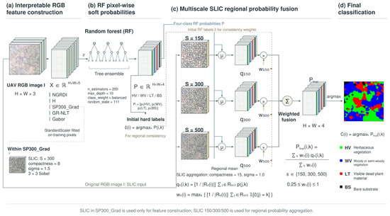
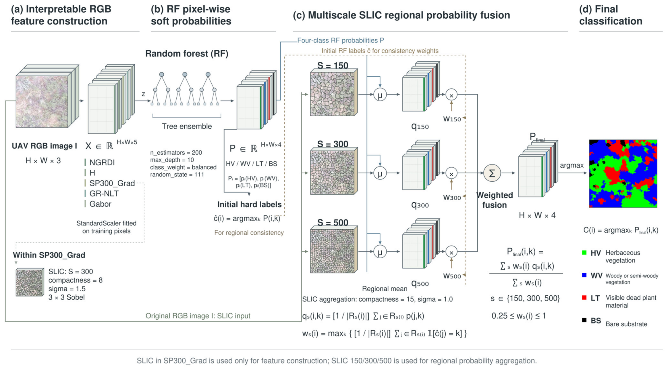
For final spatial aggregation, each 512 × 512 RGB patch was segmented using SLIC with target superpixel counts of 150, 300, and 500, representing relatively coarse, intermediate, and fine region sizes rather than fixed ground dimensions. Parameters were compactness = 15, sigma = 1.0, max_num_iter = 10, convert2lab = True, enforce_connectivity = True, min_size_factor = 0.5, max_size_factor = 3, slic_zero = False, start_label = 0, and channel_axis = −1. Connectivity constraints can cause the realized number of regions to differ from the target. These segmentations used the original RGB image, whereas the values aggregated within their regions were the RF class probabilities. The complete workflow is shown in Figure 2.

Figure 2. RF-MSPF workflow. Five RGB features supply pixelwise RF probabilities, which are averaged within SLIC regions at three scales and fused using consistency weights derived from the initial RF labels. The SLIC segmentation used to construct SP300_Grad is separate from the final probability aggregation. Arrows indicate the flow of inputs and outputs. The three branches in (c) correspond to target superpixel counts of 150, 300, and 500. Pixelwise RF probabilities are averaged within each region, and initial hard labels are used to compute consistency weights. Green, blue, red, and black in the final map denote HV, WV, LT, and BS, respectively.

We used max_num_iter = 10 as a fixed computational budget. Its influence on aggregation SLIC was assessed by comparing 10, 20, and 30 iterations while holding the other settings and the SP300_Grad feature-extraction SLIC fixed (Table S5).

Let R_s(i) denote the superpixel containing pixel i at scale s ∈ {150,300,500}. The RF probabilities for each class were averaged separately within this region:

$$q_s(i,k)={\displaystyle \frac{1}{\left|R_s\left(i\right)\right|}}{\sum }_{j\in R_s\left(i\right)}p(j,k),$$

(2)

where k denotes HV, WV, LT, or BS. Initial hard labels $\widehat{c}(j)$ were obtained by maximizing the RF pixel probabilities. Regional consistency was then defined as the fraction of pixels assigned to the most frequent predicted class in the region:

$$w_s(i)=\underset{k}{\max }\left\{{\displaystyle \frac{1}{\left|R_s(i)\right|}}{\sum }_{j\in R_s(i)}1\left[\widehat{c}(j)=\mathit{k}\right]\right\},$$

(3)

where 1 is the indicator function. For a nonempty region and four classes, the theoretical range of w_s(i) is 0.25–1. Regional probabilities from the three scales were fused as:

$$P_{\mathrm{final}}(i,k)={\displaystyle \frac{{\sum }_s{w}_s\left(i\right)q_s(i,k)}{{\sum }_s{w}_s\left(i\right)}},$$

(4)

and the final class was assigned by:

$$C(i)=\underset{k}{\arg \max }{P}_{\mathrm{final}}(i,k).$$

(5)

Setting all three scale weights to one defines MS_equal; using the consistency weights in Equation (3) defines RF-MSPF. Their direct comparison quantifies the additional contribution of consistency weighting.

2.3. Experimental Design, Evaluation, and Reproducibility

The development-oriented fixed split comprised 15 training patches and 4 validation patches, containing 247,903 and 87,772 labeled pixels, respectively. Training augmentation used the original image, horizontal flip, vertical flip, and combined flips, yielding 991,612 training samples; features were recomputed after each flip. Validation patches were unaltered. The split supported controlled spatial ablations, exploratory feature combinations, and reference-classifier comparisons. Its membership and training order were frozen in config.json, with model seed 111. It was used during earlier seed and feature exploration, and DJI_0746.JPG, DJI_0750.JPG, and DJI_0757.JPG contribute patches to both subsets (Table S3c). It is therefore a development comparison. Two training patches, patch_012 and patch_014, overlap by 27,642 source-image pixels; both are assigned to grouped-validation fold 2 (Table S3d). No same-source crop overlap crosses the fixed training–validation split.

Source-image-grouped five-fold validation used the nine analyzed source images as grouping units. GroupKFold (n_splits = 5) kept every patch from a source image in the same fold; augmentation, StandardScaler fitting, and RF training were repeated using only each training fold. The feature configuration and model parameters remained fixed from the preceding development work, rather than being selected within nested validation. Leakage and spatial dependence can inflate ecological machine-learning estimates [25,26,27]. Source grouping prevents the same source file from entering both subsets, but different photographs can still depict overlapping or adjacent ground. This within-site evaluation therefore cannot establish spatial independence or transfer to new sites, seasons, or platforms. Table S3 lists patch membership and the unequal valid-pixel counts across folds. All six spatial variants were evaluated in each fold using the same fitted RF probabilities (Table S4).

All spatial ablations shared the same RF pixel probability outputs and compared RF, S150, S300, S500, MS_equal, and RF-MSPF. This design separated the contributions of regional aggregation, scale integration, and consistency weighting. All 31 nonempty combinations of the five features were also evaluated under the same fixed development protocol, with StandardScaler and RF fitted independently for each combination and the complete spatial fusion procedure applied. This experiment is termed exploratory feature-combination analysis, not independent validation of feature selection.

Reference classifiers were RF, k-nearest neighbors (KNN), and XGBoost. KNN used n_neighbors = 15, Euclidean distance, and uniform weighting. XGBoost used n_estimators = 50, max_depth = 2, learning_rate = 0.05, eval_metric = mlogloss, and random_state = 111; other parameters followed the defaults of the fixed software version. The classifiers used the same data, 15/4 development split, five features, fourfold training augmentation, and training-fitted StandardScaler. They did not undergo independently optimized, equal-budget hyperparameter searches. Moreover, KNN and XGBoost did not receive the regional spatial post-processing used by RF-MSPF. Their results therefore provide reference performance under a unified protocol and do not establish universal classifier superiority.

Evaluation used overall accuracy (OA), average class recall (AA), Kappa, class-specific precision, recall, F1 score, and intersection over union (IoU), together with Macro-F1 and mean IoU (mIoU). Ignore pixels were excluded. Macro-F1 and mIoU weight classes equally, complementing OA, which is affected by class frequencies. Grouped five-fold OA and Macro-F1 were summarized using arithmetic means and sample standard deviations (ddof = 1). Differences across folds were interpreted descriptively, without claims of statistical significance.

The experiment used Python 3.9.6, NumPy 2.0.2, OpenCV 4.13.0, scikit-learn 1.6.1, scikit-image 0.24.0, SciPy 1.13.1, and XGBoost 1.7.6 on an Apple M4 computer with 16 GiB memory and macOS arm64. RF, KNN, and XGBoost used four workers. Per-patch timing included uncached feature calculation, standardization, RF probability prediction, three SLIC segmentations, fusion, and argmax, excluding image decoding and model loading. The supporting package contains original images and annotations, source metadata, frozen splits, full-precision outputs, and reproduction and verification scripts. Its internal output name Proposed denotes RF-MSPF. The publication tables use this mapping without changing any score. Package access is specified in the Data Availability Statement.

The iteration-sensitivity check compared segmentations of all 19 patches at three scales using adjusted Rand index (ARI). Classification reused the archived RF, training-fitted scaler, features, and probabilities on the same four validation patches and 87,772 reference pixels. All six 10-iteration predictions matched the archived arrays, isolating the effect of the aggregation-SLIC iteration budget.

3. Results

3.1. Effects of Spatial Aggregation and Overall Classification Performance

Spatial ablations using the same RF probabilities identified regional probability aggregation as the main source of improvement (Table 3). Pixel-wise RF achieved OA = 0.8412, compared with 0.8744 for S150, a gain of 3.32 percentage points. S300 and S500 achieved OA = 0.8523 and 0.8589, respectively. MS_equal achieved OA = 0.8804, exceeding the best single scale, S150, by 0.60 percentage points. RF-MSPF achieved OA = 0.8806, only 0.024 percentage points above MS_equal. Its AA, Kappa, Macro-F1, and mIoU were 0.8779, 0.8103, 0.8742, and 0.7840, respectively. Differences were calculated from unrounded results.

Table 3. Spatial ablation using the same RF pixel probability outputs.

Method	OA	AA	Kappa	Macro-F1	mIoU
RF	0.8412	0.8159	0.7488	0.8045	0.6879
S150	0.8744	0.8785	0.8015	0.8630	0.7639
S300	0.8523	0.8246	0.7663	0.8141	0.7010
S500	0.8589	0.8280	0.7763	0.8223	0.7130
MS_equal	0.8804	0.8778	0.8100	0.8732	0.7827
RF-MSPF	0.8806	0.8779	0.8103	0.8742	0.7840

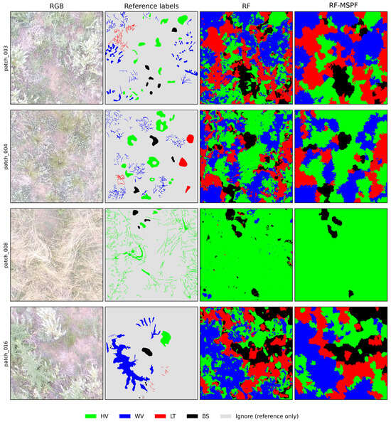
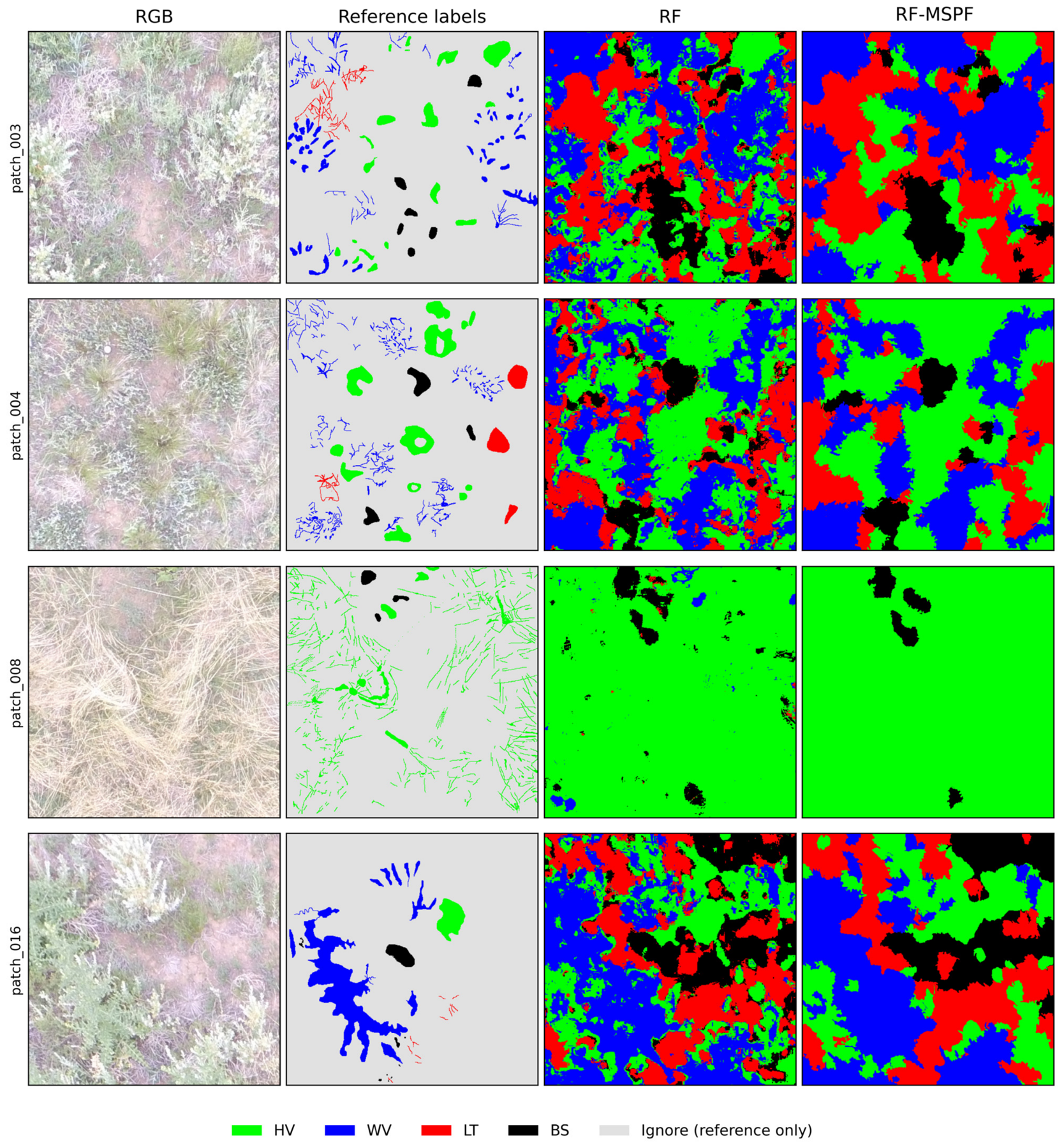
Under the unified fixed development protocol, RF, KNN, XGBoost, and RF-MSPF achieved OA values of 0.8412, 0.8307, 0.7884, and 0.8806, respectively (Table 4). Because RF-MSPF adds regional spatial processing to RF probabilities, whereas KNN and XGBoost did not receive the same post-processing, these results describe the specified configurations rather than the performance limits of independently optimized classifiers. Figure 3 compares the four development-validation patches.

Table 4. Reference classifier performance under the unified development protocol.

Method	OA	AA	Kappa	Macro-F1	mIoU
RF	0.8412	0.8159	0.7488	0.8045	0.6879
KNN	0.8307	0.7817	0.7287	0.7881	0.6689
XGBoost	0.7884	0.7550	0.6650	0.7475	0.6072
RF-MSPF	0.8806	0.8779	0.8103	0.8742	0.7840

Figure 3. RGB imagery, manual reference labels, pixel-wise RF predictions, and RF-MSPF predictions for the four development-validation patches. Green, blue, red, and black denote HV, WV, LT, and BS, respectively. Light gray indicates Ignore in the reference labels only; quantitative evaluation uses valid labeled pixels only.

3.2. Class-Specific Errors and Feature Evidence

RF-MSPF class-specific results are reported in Table 5. BS had the highest F1 and IoU, at 0.9710 and 0.9437. HV recall was 0.9395 and F1 was 0.8974. WV precision was 0.9164, whereas its recall was 0.8104. LT had precision, F1, and IoU values of 0.7354, 0.7682, and 0.6237, respectively, making it the most difficult class in this dataset.

Table 5. Class-specific RF-MSPF performance on the development-oriented fixed validation set.

Class	Valid Pixels	Precision	Recall	F1	IoU
HV	39,265	0.8589	0.9395	0.8974	0.8138
WV	34,829	0.9164	0.8104	0.8602	0.7547
LT	5975	0.7354	0.8042	0.7682	0.6237
BS	7703	0.9852	0.9573	0.9710	0.9437

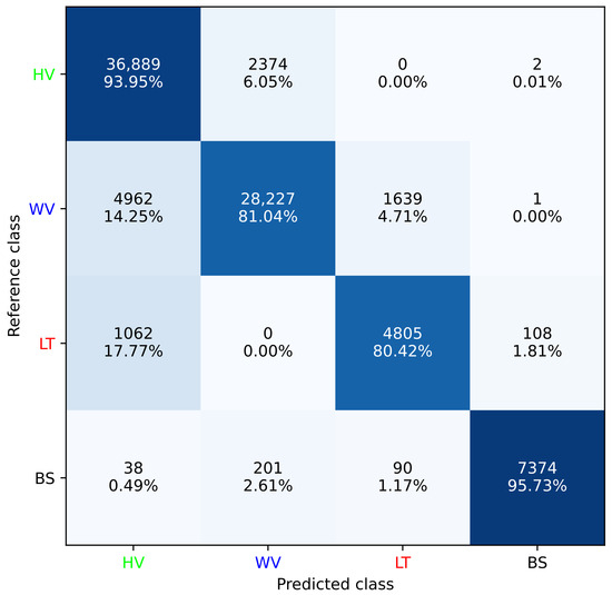
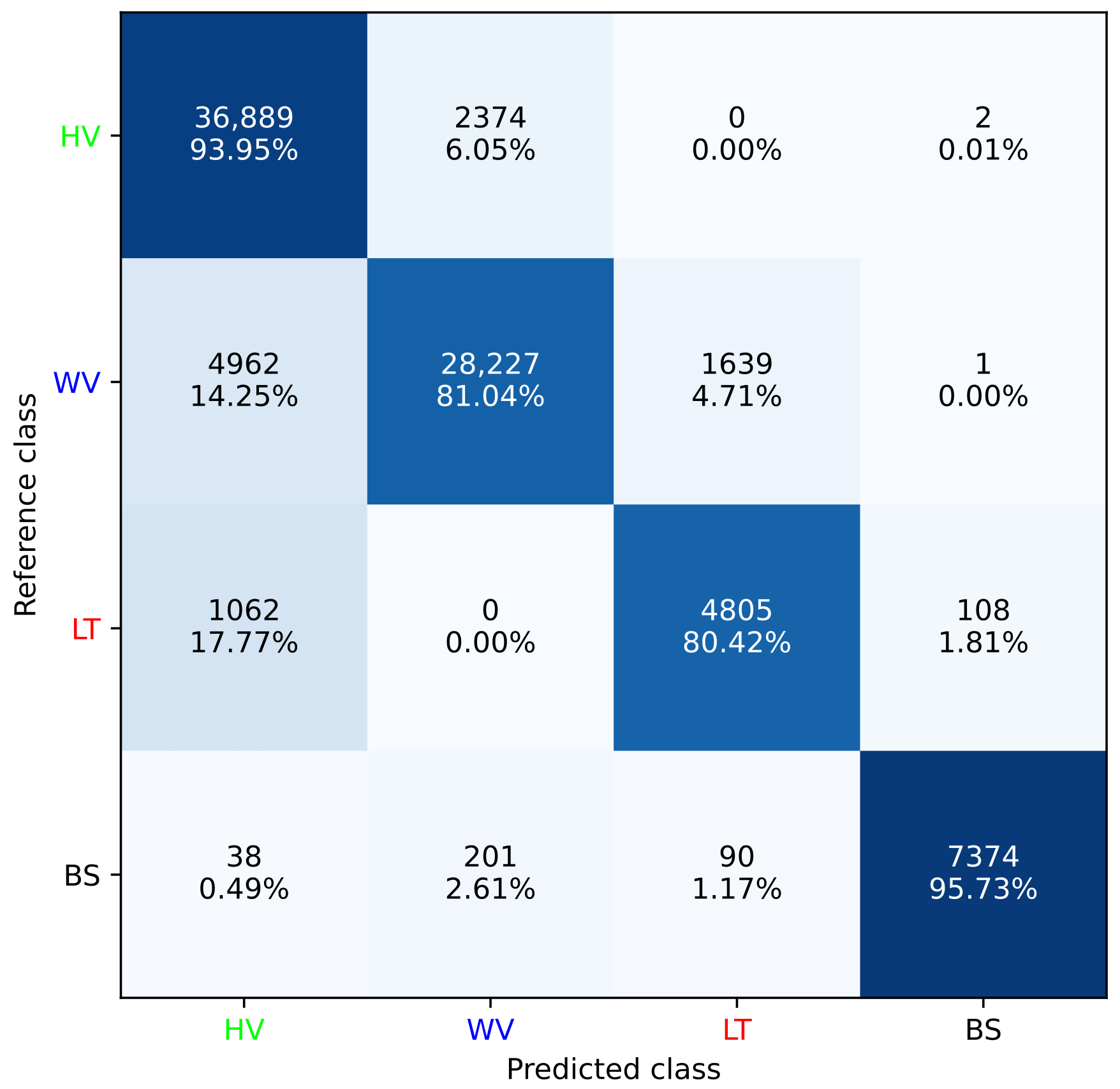
The confusion matrix showed that 14.25% of WV reference pixels were predicted as HV and 4.71% as LT; 17.77% of LT pixels were predicted as HV (Figure 4). LT → BS and BS → LT errors were 1.81% and 1.17%, respectively. Each percentage uses valid labeled pixels of the corresponding reference class as its denominator.

Figure 4. Confusion matrix for RF-MSPF on the development-oriented fixed validation set, using HV, WV, LT, and BS. In each cell, the first line gives the pixel count and the second gives the percentage normalized by the reference class. Only valid labeled pixels are included.

Among the 31 nonempty feature combinations, the complete NGRDI + H + SP300_Grad + GR-NLT + Gabor combination achieved the highest OA = 0.8806, Macro-F1 = 0.8742, and mIoU = 0.7840 on the development split. H + SP300_Grad + Gabor ranked second, with OA = 0.8619; H alone achieved OA = 0.8206. Full-precision results are provided in Table S2. These results describe combination performance under one development protocol rather than the independent causal importance of individual features.

3.3. Source-Image-Grouped Robustness and Computational Cost

RF-MSPF exceeded RF OA in all five source-image-grouped folds (Table 6). Mean OA increased from 0.8020 ± 0.0573 to 0.8691 ± 0.0367, a mean paired gain of 6.72 percentage points; Macro-F1 increased from 0.7671 ± 0.0535 to 0.8302 ± 0.0366. Equal-weight multiscale fusion achieved OA = 0.8704 ± 0.0367 and Macro-F1 = 0.8307 ± 0.0370. Consistency weighting reduced OA relative to equal weighting in three of five folds, with a mean paired difference of −0.123 percentage points. S150 achieved mean OA = 0.8686, and equal-weight multiscale fusion added 0.17 percentage points. Thus, grouped results support regional aggregation but show no consistent advantage from consistency weighting. Values after ± are sample standard deviations across folds; differences were calculated from unrounded results. All spatial variants and paired differences are reported in Table S4.

Table 6. Source-image-grouped validation with pixel-wise RF, equal fusion, and RF-MSPF. Differences are accuracy fractions; a value of 0.01 equals one percentage point. Full metrics for all six spatial variants are in Table S4.

Fold	RF OA	MS_Equal OA	RF-MSPF OA	ΔOA vs. RF	ΔOA vs. Equal
1	0.8104	0.8542	0.8490	+0.0386	−0.0051
2	0.8872	0.9298	0.9282	+0.0410	−0.0017
3	0.7393	0.8511	0.8505	+0.1113	−0.0006
4	0.7603	0.8368	0.8372	+0.0769	+0.0003
5	0.8128	0.8799	0.8809	+0.0680	+0.0010
Mean	0.8020	0.8704	0.8691	+0.0672	−0.0012
Sample SD	0.0573	0.0367	0.0367	0.0298	0.0024

On the Apple M4 CPU environment with 16 GiB memory, complete inference for a 512 × 512 patch required a mean of 0.7946 s across 12 valid timing runs, with a sample standard deviation of 0.0457 s. The combined RF and StandardScaler file occupied 27,157,561 bytes, approximately 27.16 MB. These values describe computational cost for the reported implementation and hardware.

The iteration-sensitivity comparison (Table S5) yielded mean segmentation ARI values of 0.7916 (10 versus 20 iterations), 0.7420 (10 versus 30), and 0.8860 (20 versus 30). At 10, 20, and 30 iterations, fixed-validation OA was respectively 0.8804, 0.8917, and 0.8918 for MS_equal, and 0.8806, 0.8939, and 0.8906 for RF-MSPF. The supplementary analysis shows that iteration count affects segmentation and classification. We retain the original 10-iteration setting to maintain consistency of the primary comparisons and report the longer-budget results in Table S5.

4. Discussion

4.1. Why Regional and Multiscale Information Improves Desert-Steppe Surface-Cover Mapping

Desert-steppe canopies contain leaves, branches, shadows, and visible substrate, producing local variation in color and texture. The RF baseline classifies each feature vector separately. Although SP300_Grad and Gabor already encode neighborhood information, the baseline does not explicitly average its output probabilities across neighboring pixels. Regional aggregation averages all four RF probabilities within each SLIC region, retaining relative class support rather than voting only on hard labels. On the fixed development split, S150 improved OA by 3.32 percentage points and also improved Macro-F1 and mIoU. Its grouped mean OA exceeded RF by 6.66 percentage points. These controlled comparisons identify additional output-level regional aggregation as the main contributor, consistent with the rationale for region-based vegetation mapping [15,16].

Regional aggregation can smooth local predictions but may merge fine structures when superpixels cross cover components. Figure 3 provides a qualitative comparison of spatial continuity, whereas the quantitative improvements in Table 3 apply only to valid labeled positions. With sparse reference labels, the present results do not establish improved fidelity to true boundaries.

S150 outperformed S300 and S500 on both the fixed split and grouped mean OA, indicating that coarser regional averaging was more effective for these patches. Equal-weight multiscale fusion exceeded S150 by 0.60 percentage points on the fixed split and 0.17 percentage points in grouped mean OA. These findings are compatible with complementary regional estimates but do not isolate the contribution of each finer scale.

Consistency weights measure homogeneity of the initial RF hard labels; a consistently misclassified region can therefore receive a high weight. Informative mixed transition regions may receive lower weights, while argmax-based agreement gives the same vote to weak and strong probability leads. These properties offer plausible mechanisms for the observed weighting response. Relative to equal weighting, the fixed-split OA gain was only 0.024 percentage points, whereas grouped mean OA decreased by 0.123 percentage points. Regional aggregation is consequently the principal supported contribution, while the additional benefit of consistency weighting is small and inconsistent. Both fusion results are reported to distinguish multiscale aggregation from weight design.

4.2. Ecological Interpretation and Relation to Previous UAV Studies

The five features describe green–red color relationships, hue, regional gradients, and directional texture. NGRDI and GR-NLT characterize R/G relationships, H adds hue information, SP300_Grad summarizes regional edge strength, and Gabor represents directional texture. Similar combinations of RGB indices and texture have been useful in vegetation extraction and grassland monitoring [9,10,11,12]. The full five-feature combination achieved the highest OA among the 31 combinations under the current development protocol, supporting empirical complementarity. This development-stage ranking does not establish independently optimal features across different settings.

HV and WV can both contain green foliage, limiting discrimination based on greenness alone. The 14.25% WV → HV error is consistent with visible-spectrum overlap between herbaceous tissues and woody or semi-woody canopies. Branches, canopy organization, and patch structure offer potential discrimination through gradients and texture. LT had the lowest F1 and IoU, and 17.77% of LT pixels were assigned to HV. Its varying brightness and material orientations, including standing dead herbs mixed with living tissues, shadows, and background substrate, produce substantial within-class heterogeneity. BS was comparatively stable in appearance at this site and acquisition time, with F1 = 0.9710. Although LT and BS can share yellow–brown colors, their low bidirectional confusion suggests that local morphology and texture supplied additional information in this dataset. Without class-specific causal ablations of individual features, these remain image-based interpretations consistent with the observations, not demonstrations of independent feature effects.

Shadow fraction and local intensity or texture variance offer potential supplementary descriptors for LT–HV discrimination by characterizing illumination contrasts and mixed living/dead material. Their contribution could be examined in future class-specific evaluation, accounting for exposure, substrate, and canopy geometry.

Existing UAV grassland studies differ in class definitions, sensors, and validation scales. Moreno et al. [5] segmented forage crops from RGB imagery, whereas Pranga et al. [6] combined RGB and multispectral imagery to quantify grass–clover composition. Noonan et al. [20] examined seasonal green and dead vegetation cover in rehabilitated ecosystems, and He et al. [21] used deep semantic segmentation for photosynthetic and non-photosynthetic cover in typical grasslands. Multi-sensor fusion and deep learning provide additional routes to fine-scale classification [28,29]. Differences in class definitions, reference data, spatial scale, and evaluation protocols preclude strict comparisons of reported OA. The present study does not claim that low-dimensional RF is superior to deep networks; it provides a transparent workflow for consumer-grade RGB imagery, sparse labels, and CPU computation, with spatial contributions evaluated separately.

The four classes represent surface-cover structures observable in UAV RGB imagery, not plant species or integrated ecological degradation levels. HV describes living non-woody herbaceous cover, WV maps woody or semi-woody canopies, LT represents visible dead plant material, and BS identifies exposed substrate. UAV biomass estimation, UAV–satellite mapping, and spatiotemporal transfer studies emphasize matching validation scale to intended use [4,30,31,32].

4.3. Reliability and Scope of Applicability

The study uses 19 selected patches from nine source images acquired at one site over a short period, rather than a probability sample of the landscape. The original patch-selection criteria cannot be reconstructed; Table S1 lists all 12 retained source images. Camera GPS positions do not define surveyed plot boundaries, and classification results do not represent area estimates for the entire study site.

Reference labels cover only 6.74% of the patch grids, and their spatial correlation precludes treating 335,675 labeled pixels as independent ecological observations. Labels were not independently reviewed or assessed for inter-annotator agreement; acquisition and matching records for the auxiliary near-ground photographs were not retained. Evaluation therefore describes classification at valid labeled positions.

The development split was used for seed and feature exploration and shares three source-image groups across its subsets. Comparing 31 combinations on that split introduces selection effects. Grouped validation reduces within-source reuse but does not remove possible ground overlap between different photographs, and the fixed feature set was not reselected within a nested procedure. The two overlapping crops remain together in one grouped fold. These dependencies and the small number of source groups limit conclusions to the observed dataset; the five fold scores are neither independent ecological replicates nor evidence of external generalization.

The study used one RGB camera. Illumination, shadows, automatic exposure, and white balance can affect color features, whereas sensor characteristics, acquisition height, phenology, and ground resolution can alter texture and effective region sizes. Timing and model size describe computational cost in the reported CPU environment.

The July 2025 observations support evaluation within the study site. Extending the workflow across phenological stages and regions requires attention to seasonal changes in living and dead material, canopy structure, soil appearance, and illumination, as well as geographical differences in vegetation and substrate. Independently labeled data from the target conditions would support assessment of these transfer effects.

5. Conclusions

This study developed RF-MSPF by integrating five interpretable RGB features, random forest, and multiscale superpixel probabilities to classify four desert-steppe surface-cover components: herbaceous vegetation, woody or semi-woody vegetation, visible dead plant material, and bare substrate. Using 19 patches from nine source images, source-image-grouped five-fold validation increased mean overall accuracy from 0.8020 ± 0.0573 for the RF baseline to 0.8691 ± 0.0367 for RF-MSPF (mean ± sample standard deviation), a mean paired gain of 6.72 percentage points, with improvements in every fold. On the fixed development split, RF-MSPF achieved OA = 0.8806, Macro-F1 = 0.8742, and mIoU = 0.7840. These results demonstrate that combining interpretable RGB features with regional probability information improved classification of the principal cover components within this dataset.

Spatial ablations clarified the source of the improvement. Compared with pixel-wise RF, single-scale S150 regional probability aggregation increased OA by 3.32 percentage points on the fixed development split; equal-weight multiscale fusion added a further 0.60 percentage points. Regional aggregation therefore contributed the main gain, while multiscale information provided additional improvement. Consistency weighting added only 0.024 percentage points over equal-weight fusion on that split, whereas equal-weight fusion achieved a grouped mean OA of 0.8704 ± 0.0367, slightly exceeding RF-MSPF. The principal supported methodological contribution is thus the integration of pixel-level class probabilities with multiscale regional information; consistency weighting showed no stable additional advantage.

Class-specific results on the fixed development split identified bare substrate as the most readily classified component, with F1 = 0.9710, and visible dead plant material as the most difficult, with F1 = 0.7682. The main errors involved confusion of woody or semi-woody vegetation and dead plant material with herbaceous vegetation. Overall, the study established a transparent, reproducible surface-cover classification workflow for the current UAV RGB data and identified both the main source of its improvement and differences in class discrimination. Publicly available original imagery, reference labels, analysis code, and full-precision results support verification and reproduction of these findings.

References

- Lyu, X.; Li, X.; Dang, D.; Dou, H.; Wang, K.; Lou, A. Unmanned Aerial Vehicle (UAV) Remote Sensing in Grassland Ecosystem Monitoring: A Systematic Review. Remote Sens. 2022, 14, 1096. [Google Scholar] [CrossRef] [Scilit]
- Hill, M.J.; Guerschman, J.P. Global trends in vegetation fractional cover: Hotspots for change in bare soil and non-photosynthetic vegetation. Agric. Ecosyst. Environ. 2022, 324, 107719. [Google Scholar] [CrossRef] [Scilit]
- Soubry, I.; Robinov, L.; Chu, T.; Guo, X. Mapping shrub cover in grasslands with an object-based approach and investigating the connection to topo-edaphic factors. Geocarto Int. 2022, 37, 16926–16950. [Google Scholar] [CrossRef] [Scilit]
- Chen, A.; Xu, C.; Zhang, M.; Guo, J.; Xing, X.; Yang, D.; Xu, B.; Yang, X. Cross-scale mapping of above-ground biomass and shrub dominance by integrating UAV and satellite data in temperate grassland. Remote Sens. Environ. 2024, 304, 114024. [Google Scholar] [CrossRef] [Scilit]
- Moreno, H.; Rueda-Ayala, C.; Rueda-Ayala, V.; Ribeiro, A.; Ranz, C.; Andújar, D. Machine Learning-Powered Segmentation of Forage Crops in RGB Imagery Through Artificial Sward Images. Agronomy 2025, 15, 356. [Google Scholar] [CrossRef] [Scilit]
- Pranga, J.; Borra-Serrano, I.; Quataert, P.; De Swaef, T.; Vanden Nest, T.; Willekens, K.; Ruysschaert, G.; Janssens, I.A.; Roldán-Ruiz, I.; Lootens, P. Quantification of species composition in grass-clover swards using RGB and multispectral UAV imagery and machine learning. Front. Plant Sci. 2024, 15, 1414181. [Google Scholar] [CrossRef] [Scilit]
- Hu, W.; Liu, Z.; Jia, Z.; Lock, T.R.; Kallenbach, R.L.; Yuan, Z. Rapid estimation of fractional vegetation cover in grasslands using smartphones. J. Arid. Environ. 2022, 198, 104697. [Google Scholar] [CrossRef] [Scilit]
- Bazzo, C.O.G.; Kamali, B.; Hütt, C.; Bareth, G.; Gaiser, T. A Review of Estimation Methods for Aboveground Biomass in Grasslands Using UAV. Remote Sens. 2023, 15, 639. [Google Scholar] [CrossRef] [Scilit]
- Pham, D.; Gautam, D.; Sheffield, K. Classifying Serrated Tussock Cover from Aerial Imagery Using RGB Bands, RGB Indices, and Texture Features. Remote Sens. 2024, 16, 4538. [Google Scholar] [CrossRef] [Scilit]
- Dong, J.; Zhang, J.; Zhang, S.; Yu, Z.; Song, Z.; Meng, T. Vegetation extraction through UAV RGB imagery and efficient feature selection. PLoS ONE 2025, 20, e0322180. [Google Scholar] [CrossRef] [Scilit]
- Ye, X.; Zhu, W.; Liu, R.; He, B.; Yang, X.; Zhao, C. An automated method for estimating fractional vegetation cover from camera-based field measurements: Saturation-adaptive threshold for ExG (SATE). ISPRS J. Photogramm. Remote Sens. 2025, 229, 170–187. [Google Scholar] [CrossRef] [Scilit]
- Pan, T.; Ye, H.; Zhang, X.; Liao, X.; Wang, D.; Bayin, D.; Safarov, M.; Okhonniyozov, M.; Majid, G. Estimating aboveground biomass of grassland in central Asia mountainous areas using unmanned aerial vehicle vegetation indices and image textures—A case study of typical grassland in Tajikistan. Environ. Sustain. Indic. 2024, 22, 100345. [Google Scholar] [CrossRef] [Scilit]
- Huang, L.; Zhao, F.; Hu, G.; Ganjurjav, H.; Wu, R.; Gao, Q. Evaluation of Machine Learning Models for Estimating Grassland Pasture Yield Using Landsat-8 Imagery. Agronomy 2024, 14, 2984. [Google Scholar] [CrossRef] [Scilit]
- Zhao, J.; Li, K.; Zhang, J.; Liu, Y.; Li, X. Mapping Invasive Species Pedicularis and Background Grassland Using UAV and Machine Learning Algorithms. Drones 2024, 8, 639. [Google Scholar] [CrossRef] [Scilit]
- Ventura, D.; Napoleone, F.; Cannucci, S.; Alleaume, S.; Valentini, E.; Casoli, E.; Burrascano, S. Integrating low-altitude drone based-imagery and OBIA for mapping and manage semi natural grassland habitats. J. Environ. Manag. 2022, 321, 115723. [Google Scholar] [CrossRef] [Scilit]
- Costa, L.S.; Sano, E.E.; Ferreira, M.E.; Munhoz, C.B.R.; Costa, J.V.S.; Rufino Alves Júnior, L.; de Mello, T.R.B.; da Cunha Bustamante, M.M. Woody Plant Encroachment in a Seasonal Tropical Savanna: Lessons about Classifiers and Accuracy from UAV Images. Remote Sens. 2023, 15, 2342. [Google Scholar] [CrossRef] [Scilit]
- Achanta, R.; Shaji, A.; Smith, K.; Lucchi, A.; Fua, P.; Süsstrunk, S. SLIC Superpixels Compared to State-of-the-Art Superpixel Methods. IEEE Trans. Pattern Anal. Mach. Intell. 2012, 34, 2274–2282. [Google Scholar] [CrossRef] [Scilit]
- Huang, S.; Liu, Z.; Jin, W.; Mu, Y. Superpixel-based multi-scale multi-instance learning for hyperspectral image classification. Pattern Recognit. 2024, 149, 110257. [Google Scholar] [CrossRef] [Scilit]
- Ayres, L.C.; de Almeida, S.J.M.; Bermudez, J.C.M.; Borsoi, R.A. Hierarchical homogeneity-based superpixel segmentation: Application to hyperspectral image analysis. Int. J. Remote Sens. 2024, 45, 6004–6042. [Google Scholar] [CrossRef] [Scilit]
- Noonan, M.; He, Y.; Nelson, D.; Ge, H.; Siu, R.; Duval, T.P. Estimating seasonal fractional green and dead vegetation cover in rehabilitated ecosystems using drone remote sensing. Ecol. Inform. 2025, 92, 103456. [Google Scholar] [CrossRef] [Scilit]
- He, J.; Zhang, X.; Li, W.; Lyu, D.; Ren, Y.; Fu, W. Extraction of Photosynthetic and Non-Photosynthetic Vegetation Cover in Typical Grasslands Using UAV Imagery and an Improved SegFormer Model. Remote Sens. 2025, 17, 3162. [Google Scholar] [CrossRef] [Scilit]
- Li, J.; He, B.; Zhou, S.; Zhang, X.; Li, C.; Han, G. Prediction of plant diversity under different stocking rates based on functional traits of constructive species in a desert steppe, northern China. Front. Ecol. Evol. 2022, 10, 865703. [Google Scholar] [CrossRef] [Scilit]
- Bai, L.; Wang, J.; Wang, Z.; Li, Z.; Ren, H.; Wang, H.; Zhang, G.; Han, G. Effects of simulated precipitation gradients on nutrient resorption in the desert steppe of northern China. Front. Plant Sci. 2023, 14, 1211182. [Google Scholar] [CrossRef] [Scilit]
- Breiman, L. Random Forests. Mach. Learn. 2001, 45, 5–32. [Google Scholar] [CrossRef] [Scilit]
- Stock, A.; Gregr, E.J.; Chan, K.M.A. Data leakage jeopardizes ecological applications of machine learning. Nat. Ecol. Evol. 2023, 7, 1743–1745. [Google Scholar] [CrossRef] [Scilit]
- Bernett, J.; Blumenthal, D.B.; Grimm, D.G.; Haselbeck, F.; Joeres, R.; Kalinina, O.V.; List, M. Guiding questions to avoid data leakage in biological machine learning applications. Nat. Methods 2024, 21, 1444–1453. [Google Scholar] [CrossRef] [Scilit]
- Koldasbayeva, D.; Tregubova, P.; Gasanov, M.; Zaytsev, A.; Petrovskaia, A.; Burnaev, E. Challenges in data-driven geospatial modeling for environmental research and practice. Nat. Commun. 2024, 15, 10700. [Google Scholar] [CrossRef] [Scilit] [PubMed]
- Cai, Z.; Wen, C.; Bao, L.; Ma, H.; Yan, Z.; Li, J.; Gao, X.; Yu, L. Fine-Scale Grassland Classification Using UAV-Based Multi-Sensor Image Fusion and Deep Learning. Remote Sens. 2025, 17, 3190. [Google Scholar] [CrossRef] [Scilit]
- Sotomayor, L.N.; Lucieer, A.; Turner, D.; Lewis, M.; Kattenborn, T. Mapping fractional vegetation cover in UAS RGB and multispectral imagery in semi-arid Australian ecosystems using CNN-based semantic segmentation. Landsc. Ecol. 2025, 40, 169. [Google Scholar] [CrossRef] [Scilit]
- Cao, L.; Fu, Y.; Zhao, T.; Meng, D.; Pan, X.; Sun, W. UAV-based aboveground biomass estimation via trait-mediated pathways in a cultivated Leymus chinensis grassland. J. Environ. Manag. 2026, 402, 129164. [Google Scholar] [CrossRef] [Scilit]
- Amputu, V.; Männer, F.; Tielbörger, K.; Knox, N. Spatio-Temporal Transferability of Drone-Based Models to Predict Forage Supply in Drier Rangelands. Remote Sens. 2024, 16, 1842. [Google Scholar] [CrossRef] [Scilit]
- Martínez Prentice, R.; Villoslada, M.; Ward, R.D.; Bergamo, T.F.; Joyce, C.B.; Sepp, K. Synergistic use of Sentinel-2 and UAV-derived data for plant fractional cover distribution mapping of coastal meadows with digital elevation models. Biogeosciences 2024, 21, 1411–1431. [Google Scholar] [CrossRef] [Scilit]
Disclaimer/Publisher’s Note: The statements, opinions and data contained in all publications are solely those of the individual author(s) and contributor(s) and not of MDPI and/or the editor(s). MDPI and/or the editor(s) disclaim responsibility for any injury to people or property resulting from any ideas, methods, instructions or products referred to in the content. |
© 2026 by the authors. Licensee MDPI, Basel, Switzerland. This article is an open access article distributed under the terms and conditions of the Creative Commons Attribution (CC BY) license.