Superconfined Antiferromagnons on the Two-Dimensional Penrose Lattice

Abstract

We find novel confined states in the spin-S nearest-neighbor antiferromagnetic Heisenberg model on the two-dimensional Penrose lattice. Linear spin waves have massively degenerate eigenstates strictly confined to tricoordinated sites. They contrast with the well-known itinerant analogs in the tight-binding model, where electrons are confined but extended to both tricoordinated and pentacoordinated sites. It is the site potentials in the spin-wave Hamiltonian, originating from Coulomb interactions between electrons, that confine spin waves to minimally coordinated sites only. Confined states in the tight-binding Hamiltonian consist of six types of building blocks, whereas those in the spin-wave Hamiltonian consist of only four of them. Confined spin waves are robust against 1/S corrections. Emergent O(S⁰) interactions further confine—superconfine—spin waves into two separate groups within tricoordinated sites.

1. Introduction

Quasicrystals have aperiodic but long-range ordered atomic arrangements [1,2] to exhibit non-crystallographic rotational symmetry and self-similarity. Since the discovery of such a structure in an Al-Mn alloy [3], numerous transition-metal alloys have been tried and proved to be quasicrystalline [4,5,6,7]. In particular, magnetic long-range order was reported in rare-earth-based icosahedral quasicrystals, namely ferromagnetic order in Au-Ga-R (R = Gd, Tb, and Dy) [8,9] and antiferromagnetic order in Au-In-Eu [10], confirmed by neutron diffraction and magnetization measurements. These findings have provided a conclusive answer to the long-standing question of whether magnetic long-range order can emerge in quasicrystals [11,12,13,14,15]. Motivated by the observations of magnetic long-range order, as well as quantum criticality [16], superconductivity [17], and related phenomena, theoretical studies based on ideal models are essential for understanding how aperiodic geometry governs collective excitations [18,19,20,21,22,23,24].

The ${\mathbf{C}}_{5\mathrm{v}}$ Penrose tiling [25] is a two-dimensional realization of quasiperiodicity. It not only deserves investigation in itself but also serves as an ideal platform for exploring quasicrystals, especially of icosahedral point group symmetry. A striking feature of its electronic structure is the macroscopic degeneracy of the tight-binding Hamiltonian in the vertex model, where electrons hop between adjacent vertices connected by rhombus edges [26,27]. This Hamiltonian hosts a macroscopically degenerate zero-energy eigenlevel [28,29,30,31,32,33,34], which originates from a set of distinctive eigenstates known as confined states, whose wavefunctions are strictly confined to finite domains. These states are critical in nature—neither localized nor extended in the conventional sense—as they lack any characteristic length scale. Arai et al. proposed that the confined states are composed of six independent building blocks [29], which was numerically demonstrated indeed [34].

Macroscopic zero-energy degeneracy is found in various quasiperiodic tight-binding models as well, such as the generalized Penrose lattice [35], Ammann–Beenker lattice [36,37], Socolar dodecagonal lattice [38,39], hexagonal golden-mean tilings [40,41], quasiperiodic twisted bilayer systems [42], and the recently discovered aperiodic monotile [43]. Confined states do not necessarily occur at zero energy but can emerge at nonzero energies as well. In the center model on the Penrose lattice, with an s-like orbital placed at the center of each rhombus, non-interacting electrons exhibit confined states at energy $2t$ [44,45,46], where t is the hopping integral. In the $\pi$-flux model on the Ammann–Beenker lattice, confined states appear at energies $\pm \sqrt{2}t$, $\pm 2t$, and $\pm 2\sqrt{2}t$, as well as at zero energy, depending on flux configurations [47].

While such macroscopic degeneracy has been extensively studied in electron hopping models, analogous phenomena occur in spin systems as well. The half-filled single-band Hubbard model maps onto a spin $-{\displaystyle \frac{1}{2}}$ Heisenberg antiferromagnet in the strong correlation limit [48,49]. Quantum Monte Carlo (QMC) simulations reveal that the spatially averaged staggered magnetization for the Penrose-lattice Heisenberg antiferromagnet is larger than that of the square lattice, despite both having the same average coordination number of four [50,51,52]. This suggests that the structural inhomogeneity suppresses quantum fluctuations. The local magnetizations obtained from linear spin-wave (LSW) theory qualitatively agree with the QMC results in terms of their coordination-number dependence, and the ground-state energies from LSW and QMC calculations also agree to within $2\%$ [50,53]. Spin dynamics has also been investigated via inelastic photon [54,55] and neutron [56] scattering calculations. Within the harmonic-oscillator approximation for the Heisenberg antiferromagnet on the Penrose lattice, a prominent peak appears in the density of states at energy $3JS$ [53], where J is the exchange interaction, and S is the spin magnitude. At this energy, numerous degenerate states emerge, characterized by string-like wavefunctions that form closed loops without a characteristic length scale. These states manifest as nearly flat-band excitations in the dynamic structure factor, spanning almost the entire momentum space [56]. A perpendicular-space [57] analysis attributes their origin to antiferromagnons strongly confined to tricoordinated sites.

We demonstrate that the macroscopically degenerate spin-wave excitations in the Penrose-lattice Heisenberg antiferromagnet are confined states of antiferromagnons—the magnetic analogs of the well-known confined states in the tight-binding model.

2. Model and Method

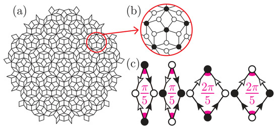
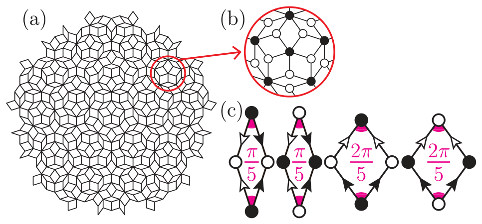
We consider the spin-S nearest-neighbor antiferromagnetic Heisenberg model on the two-dimensional Penrose lattice, which consists of bipartite sublattices A and B (Figure 1). The Hamiltonian reads

$$\begin{array}{c}\hfill \mathcal{H}=J\sum _{i\in \mathrm{A}}\sum _{j\in \mathrm{B}}{l}_{i,j}{\mathit{S}}_{{\mathit{r}}_i}·{\mathit{S}}_{{\mathit{r}}_j}(J>0).\end{array}$$

(1)

We denote the vector spin operators on the A and B sublattices by ${\mathit{S}}_{{\mathit{r}}_i}$ ($i=1,2,\dots ,L_{\mathrm{A}}$) and ${\mathbf{S}}_{{\mathit{r}}_j}$$(j=1,2,\dots ,L_{\mathrm{B}})$, respectively, where ${\mathit{r}}_l$ serves as a generic site label running over both sublattices. The total number of sites is $L=L_{\mathrm{A}}+L_{\mathrm{B}}$. The linkage identifier $l_{i,j}$ equals 1 if the vertices ${\mathit{r}}_i$ and ${\mathit{r}}_j$ are connected, and 0 otherwise. We express the Hamiltonian (1) in terms of the Holstein–Primakoff bosons [58],

$$\begin{array}{cc}\hfill & S_{{\mathit{r}}_i}^{+}={\left(2S-a_i^{†}{a}_i\right)}^{{\displaystyle \frac{1}{2}}}{a}_i,S_{{\mathit{r}}_i}^{-}=a_i^{†}{\left(2S-a_i^{†}{a}_i\right)}^{{\displaystyle \frac{1}{2}}},S_{{\mathit{r}}_i}^z=S-a_i^{†}{a}_i,\hfill \\ \hfill & S_{{\mathit{r}}_j}^{+}=b_j^{†}{\left(2S-b_j^{†}{b}_j\right)}^{{\displaystyle \frac{1}{2}}},S_{{\mathit{r}}_j}^{-}={\left(2S-b_j^{†}{b}_j\right)}^{{\displaystyle \frac{1}{2}}}{b}_j,S_{{\mathit{r}}_j}^z=b_j^{†}{b}_j-S,\hfill \end{array}$$

(2)

and expand it in descending powers of S [59],

$$\begin{array}{c}\hfill \mathcal{H}={\mathcal{H}}^{\left(2\right)}+{\mathcal{H}}^{\left(1\right)}+O\left(S^0\right),\end{array}$$

(3)

where ${\mathcal{H}}^{\left(m\right)}$, on the order of $S^m$, reads

$$\begin{array}{cc}\hfill & {\mathcal{H}}^{\left(2\right)}=-J{S}^2\sum _{i\in \mathrm{A}}\sum _{j\in \mathrm{B}}{l}_{i,j},{\mathcal{H}}^{\left(1\right)}=JS\sum _{i\in \mathrm{A}}\sum _{j\in \mathrm{B}}{l}_{i,j}\left(a_i^{†}{a}_i+b_j^{†}{b}_j+a_i{b}_j+a_i^{†}{b}_j^{†}\right).\hfill \end{array}$$

(4)

We define the up-to-$O\left(S^1\right)$ LSW Hamiltonian

$$\begin{array}{c}\hfill {\mathcal{H}}^{\left[1\right]}\equiv {\mathcal{H}}^{\left(2\right)}+{\mathcal{H}}^{\left(1\right)}.\end{array}$$

(5)

Figure 1. (a) A two-dimensional Penrose lattice with size $L=526$ and (b) an enlarged view of a specific region. The open and filled circles represent sites belonging to the two sublattices. (c) Two types of rhombic prototiles constituting the Penrose lattice, with acute angles of ${\displaystyle \frac{\pi }{5}}$ (thin) and ${\displaystyle \frac{2\pi }{5}}$ (fat). Each edge is marked with an arrow to define the matching rules. For each prototile, there are two possible sublattice assignments at the vertices.

We introduce the row vectors ${\mathit{d}}^{†}$, ${\mathit{a}}^{†}$, and ${}^t\mathit{b}$, of dimension L, $L_{\mathrm{A}}$, and $L_{\mathrm{B}}$, respectively, as

$$\begin{array}{c}\hfill {\mathit{d}}^{†}=\left[a_1^{†},\dots ,a_{L_{\mathrm{A}}}^{†},b_1,\dots ,b_{L_{\mathrm{B}}}\right]\equiv \left[{\mathit{a}}^{†},{}^t\mathit{b}\right].\end{array}$$

(6)

Then, we can compactly express the LSW Hamiltonian in matrix form as

$$\begin{array}{cc}\hfill & {\mathcal{H}}^{\left[1\right]}={\mathcal{H}}^{\left(2\right)}+{\epsilon }^{\left(1\right)}+JS\left[{\mathit{a}}^{†},{}^t\mathit{b}\right]\left[\begin{array}{cc}{\mathbf{Z}}_{\mathrm{AA}}& {\mathbf{C}}_{\mathrm{AB}}\\ {\mathbf{C}}_{\mathrm{AB}}^{†}& {\mathbf{Z}}_{\mathrm{BB}}\end{array}\right]\left[\begin{array}{c}\mathit{a}\\ {}^t\mathit{b}^{†}\end{array}\right]\hfill \\ \hfill & \equiv {\mathcal{H}}^{\left(2\right)}+{\epsilon }^{\left(1\right)}+JS{\mathit{d}}^{†}\mathbf{M}\mathit{d};{\epsilon }^{\left(1\right)}=-JS\sum _{i\in \mathrm{A}}\sum _{j\in \mathrm{B}}{l}_{i,j},\hfill \end{array}$$

(7)

where ${\mathbf{Z}}_{\mathrm{AA}}$ and ${\mathbf{Z}}_{\mathrm{BB}}$ are diagonal matrices of dimension $L_{\mathrm{A}}\times L_{\mathrm{A}}$ and $L_{\mathrm{B}}\times L_{\mathrm{B}}$, respectively, and ${\mathbf{C}}_{\mathrm{AB}}$ is the biadjacency matrix of dimension $L_{\mathrm{A}}\times L_{\mathrm{B}}$, as

$$\begin{array}{c}\hfill {\left[{\mathbf{Z}}_{\mathrm{AA}}\right]}_{i,i^{\prime }}=z_i{\delta }_{i,i^{\prime }},{\left[{\mathbf{Z}}_{\mathrm{BB}}\right]}_{j,j^{\prime }}=z_j{\delta }_{j,j^{\prime }},{\left[{\mathbf{C}}_{\mathrm{AB}}\right]}_{i,j}=l_{i,j},\end{array}$$

(8)

where $z_l$ is the coordination number of the site at ${\mathit{r}}_l$. Denoting the diagonal and off-diagonal blocks of the LSW Hamiltonian matrix $\mathbf{M}$ as

$$\begin{array}{c}\hfill \mathbf{Z}\equiv \left[\begin{array}{cc}{\mathbf{Z}}_{\mathrm{AA}}& {\mathbf{O}}_{\mathrm{AB}}\\ {\mathbf{O}}_{\mathrm{AB}}^{†}& {\mathbf{Z}}_{\mathrm{BB}}\end{array}\right],\mathbf{T}\equiv \left[\begin{array}{cc}{\mathbf{O}}_{\mathrm{AA}}& {\mathbf{C}}_{\mathrm{AB}}\\ {\mathbf{C}}_{\mathrm{AB}}^{†}& {\mathbf{O}}_{\mathrm{BB}}\end{array}\right],\end{array}$$

(9)

where ${\mathbf{O}}_{\mathrm{AA}}$, ${\mathbf{O}}_{\mathrm{BB}}$, and ${\mathbf{O}}_{\mathrm{AB}}$ are zero matrices of dimension $L_{\mathrm{A}}\times L_{\mathrm{A}}$, $L_{\mathrm{B}}\times L_{\mathrm{B}}$, and $L_{\mathrm{A}}\times L_{\mathrm{B}}$, respectively, we obtain

$$\begin{array}{c}\hfill \mathbf{M}=\mathbf{Z}+\mathbf{T}.\end{array}$$

(10)

We carry out the Bogoliubov transformation [60,61]

$$\begin{array}{cc}\hfill & \mathit{d}=\left[\begin{array}{cc}\mathbf{V}& \mathbf{X}\\ \mathbf{Y}& \mathbf{W}\end{array}\right]\mathit{\alpha };{\left[\mathbf{V}\right]}_{i,k_{-}}=v_{i,k_{-}},{\left[\mathbf{W}\right]}_{j,k_{+}}=w_{j,k_{+}},{\left[\mathbf{X}\right]}_{i,k_{+}}=x_{i,k_{+}},{\left[\mathbf{Y}\right]}_{j,k_{-}}=y_{j,k_{-}}\hfill \end{array}$$

(11)

with the matrices $\mathbf{V}$, $\mathbf{W}$, $\mathbf{X}$, and $\mathbf{Y}$, of dimension $L_{\mathrm{A}}\times L_{-}$, $L_{\mathrm{B}}\times L_{+}$, $L_{\mathrm{A}}\times L_{+}$, and $L_{\mathrm{B}}\times L_{-}$, respectively, to obtain quasiparticle magnons

$$\begin{array}{c}\hfill \left[{\alpha }_1^{-†},\dots ,{\alpha }_{L_{-}}^{-†},{\alpha }_1^{+},\dots ,{\alpha }_{L_{+}}^{+}\right]\equiv {\mathit{\alpha }}^{†}\end{array}$$

(12)

and the diagonalized LSW Hamiltonian

$$\begin{array}{c}\hfill {\mathcal{H}}^{\left[1\right]}={\mathcal{H}}^{\left(2\right)}+{\epsilon }^{\left(1\right)}+{\displaystyle \sum _{k_{+}=1}^{L_{+}}}{\epsilon }_{k_{+}}^{+}+\sum _{\sigma =\mp }{\displaystyle \sum _{k_{\sigma }=1}^{L_{\sigma }}}{\epsilon }_{k_{\sigma }}^{\sigma }{\alpha }_{k_{\sigma }}^{\sigma †}{\alpha }_{k_{\sigma }}^{\sigma },\end{array}$$

(13)

where ${\alpha }_{k_{\sigma }}^{\sigma †}$ creates a ferromagnetic ($\sigma =-$) or antiferromagnetic ($\sigma =+$) magnon of energy ${\epsilon }_{k_{\sigma }}^{\sigma }$.

We define the site-resolved density of states for the quasiparticle magnon excitation spectrum

$$\begin{array}{cc}\hfill & \rho \left(\omega \right)={\displaystyle \sum _{l=1}^L}{\rho }_l\left(\omega \right)={\displaystyle \sum _{z=3}^7}{\rho }_z\left(\omega \right)={\displaystyle \sum _{z=3}^7}{\displaystyle \frac{1}{L}}\left\{{\displaystyle \sum _{k_{-}=1}^{L_{-}}}{\displaystyle \frac{{\sum }_{i(z_i=z)}{\left|v_{i,k_{-}}\right|}^2+{\sum }_{j(z_j=z)}{\left|y_{j,k_{-}}\right|}^2}{{\sum }_{i\in \mathrm{A}}{\left|v_{i,k_{-}}\right|}^2+{\sum }_{j\in \mathrm{B}}{\left|y_{j,k_{-}}\right|}^2}}\delta \left(\hslash \omega -{\epsilon }_{k_{-}}^{-}\right)\right.\hfill \\ \hfill & \left.+{\displaystyle \sum _{k_{+}=1}^{L_{+}}}{\displaystyle \frac{{\sum }_{i(z_i=z)}{\left|x_{i,k_{+}}\right|}^2+{\sum }_{j(z_j=z)}{\left|w_{j,k_{+}}\right|}^2}{{\sum }_{i\in \mathrm{A}}{\left|x_{i,k_{+}}\right|}^2+{\sum }_{j\in \mathrm{B}}{\left|w_{j,k_{+}}\right|}^2}}\delta \left(\hslash \omega -{\epsilon }_{k_{+}}^{+}\right)\right\}.\hfill \end{array}$$

(14)

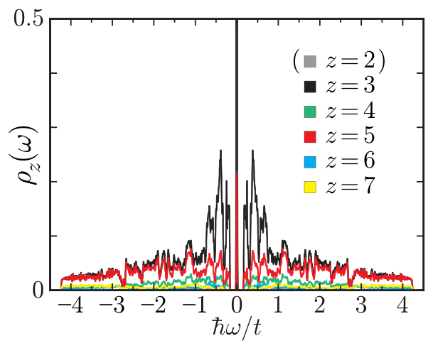
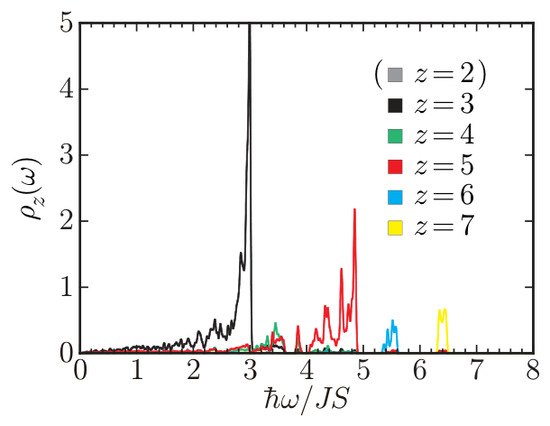
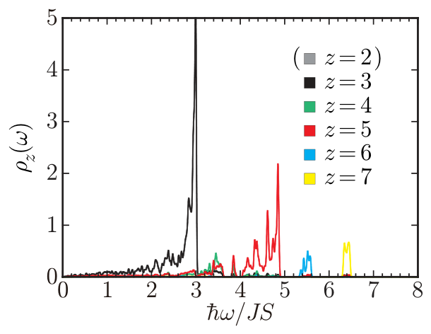
Figure 2 shows the coordination-number-resolved density of states ${\rho }_z\left(\omega \right)$, where z ranges from 3 to 7 (see Appendix A). The spectral weight shifts toward sites with higher coordination numbers as the energy increases, a feature attributable to the immobility of spin deviations in the Ising limit. In this limit, the excitation spectrum consists of discrete eigenlevels at $zJS$. The correlation between coordination number and excitation energy persists even when the degeneracy is lifted by spin fluctuations. Notably, the sharp peak at $\hslash \omega =3JS$ indicates macroscopically degenerate confined states.

Figure 2. The coordination-number-resolved density of states ${\rho }_z\left(\omega \right)$ for the LSW excitation spectrum on the Penrose lattice with L = 11,006, where z ranges from 3 to 7. Note that $z=2$ vertices are artifacts of finite open-boundary clusters.

3. Confined Antiferromagnons

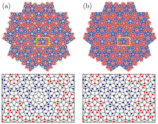
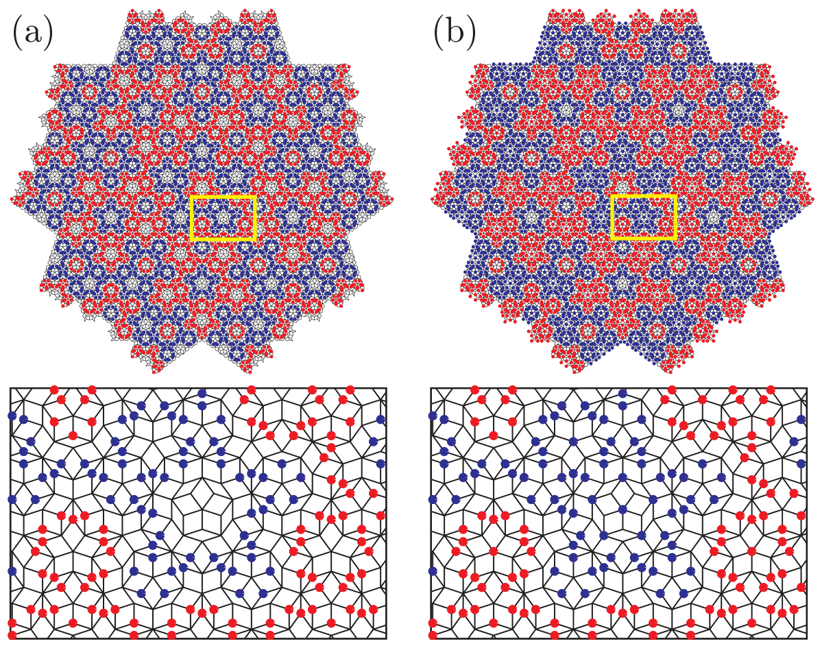
Figure 3 demonstrates the spatial confinement of degenerate states at ${\epsilon }_k^{\mp }=3JS$ for the LSW Hamiltonian and at ${\epsilon }_k=0$ for the tight-binding Hamiltonian (see Appendix B) on the Penrose lattice. Here, ${\epsilon }_k$ denotes the eigenvalues of the tight-binding Hamiltonian. In both cases, these confined states are spatially separated by “forbidden ladders” [29,34], which are one-dimensional, unbranched closed loops with zero wavefunction amplitude. Within each domain enclosed by these forbidden ladders, the confined states exhibit nonzero amplitudes exclusively on either the A or B sublattice. The alternating pattern of confinement domains across the forbidden ladders matches perfectly between Figure 3a,b. A key distinction between the two types of confined states lies in their spatial distributions: in the LSW eigenstates (Figure 3a), antiferromagnons are confined only to tricoordinated sites, whereas in the tight-binding eigenstates (Figure 3b), electrons are confined to tricoordinated and pentacoordinated sites.

Figure 3. The site-resolved densities of states ${\rho }_l\left(\omega \right)$ [Equations (14) and (A8)] multiplied by the number of sites L = 11,006 as functions of site position ${\mathit{r}}_l$. The lth site is marked with a red ($l\in \mathrm{A}$) or blue ($l\in \mathrm{B}$) dot when $L{\rho }_l\left(\omega \right)$ is larger than or equal to ${10}^{-2}$. At every unmarked site l, $L{\rho }_l\left(\omega \right)<{10}^{-15}$. (a) $L{\rho }_l\left(\omega \right)$ at $\hslash \omega =3JS$ for the LSW Hamiltonian (13). (b) $L{\rho }_l\left(\omega \right)$ at $\hslash \omega =0$ for the tight-binding Hamiltonian (A7). Rectangles highlight regions enlarged in the bottom panels and in Figure A5.

We derive the constraints on the wavefunction amplitudes of the confined states. The matrix form of the LSW Hamiltonian (7) reduces the problem to an eigenvalue problem for the matrix $\mathbf{M}=\mathbf{Z}+\mathbf{T}$. We first examine the off-diagonal connectivity matrix $\mathbf{T}$, which corresponds to the tight-binding Hamiltonian with the hopping integral set to unity. Using the argument from the tight-binding model (see Appendix B), we obtain the local constraints at each site ${\mathit{r}}_l$ for the LSW wavefunction (11) to be an eigenvector of $\mathbf{T}$ with zero eigenvalue, which read

$$\begin{array}{c}\hfill \left\{\begin{array}{cc}{\displaystyle \sum _{j\in \mathrm{B}}}{l}_{i,j}{y}_{j,k_{-}}=0\hfill & (l=i\in \mathrm{A})\hfill \\ {\displaystyle \sum _{i\in \mathrm{A}}}{l}_{i,j}{v}_{i,k_{-}}=0\hfill & (l=j\in \mathrm{B})\hfill \end{array}\right.\end{array}$$

(15)

for the $\sigma =-$ mode and

$$\begin{array}{c}\hfill \left\{\begin{array}{cc}{\displaystyle \sum _{j\in \mathrm{B}}}{l}_{i,j}{w}_{j,k_{+}}=0\hfill & (l=i\in \mathrm{A})\hfill \\ {\displaystyle \sum _{i\in \mathrm{A}}}{l}_{i,j}{x}_{i,k_{+}}=0\hfill & (l=j\in \mathrm{B})\hfill \end{array}\right.\end{array}$$

(16)

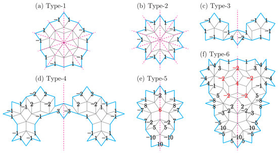
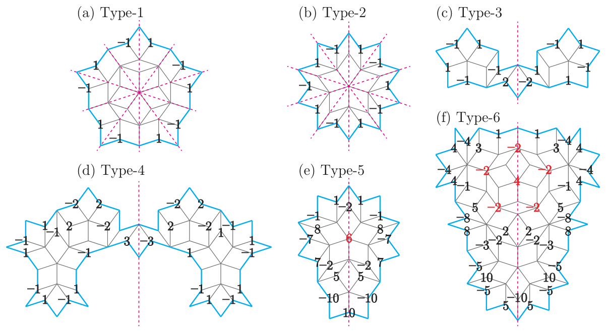
for the $\sigma =+$ mode. As established in Refs. [29,34], for the connectivity matrix $\mathbf{T}$ on the infinite Penrose lattice, the only local solutions satisfying Equations (15) and (16) are the six types of building blocks shown in Figure 4. We define the L-dimensional vector

$$\begin{array}{c}\hfill {\mathit{\psi }}_{n,m}=\left[\begin{array}{c}{\psi }_{n,m}\left({\mathit{r}}_1\right)\\ ⋮\\ {\psi }_{n,m}\left({\mathit{r}}_L\right)\end{array}\right],{\left[{\mathit{\psi }}_{n,m}\right]}_l={\psi }_{n,m}\left({\mathit{r}}_l\right),\end{array}$$

(17)

where $n=1,\dots ,6$ labels the type of building block, $m=1,\dots ,N_n$ labels each block of type-n, and $N_n$ is the total number of such blocks. Each ${\mathit{\psi }}_{n,m}$ is an unnormalized eigenvector of $\mathbf{T}$ satisfying $\mathbf{T}{\mathit{\psi }}_{n,m}=0$. The wavefunction amplitudes ${\psi }_{n,m}\left({\mathit{r}}_l\right)$ at each site take the values specified in Figure 4 for the corresponding tiles of the Penrose lattice and are zero elsewhere. The number of nonzero components for each type of building block is summarized in Table 1.

Figure 4. Six types of building blocks for the zero-eigenvalue states of the connectivity matrix $\mathbf{T}$ on the two-dimensional Penrose lattice. Numbers on the vertices indicate the relative amplitude of the unnormalized wavefunctions (black: $z=3$ vertices; red: $z=5$ vertices). Vertices without numbers have zero amplitude. Dotted lines denote mirror-symmetry axes. Type-1 to type-4 wavefunctions are mirror-antisymmetric, while type-5 and type-6 wavefunctions are mirror-symmetric. Type-1 and type-2 building blocks exhibit fivefold rotational symmetry. Note that the tiles of type-4 and type-5 include those of type-3 and type-2, respectively, and the tiles of type-6 include those of type-1 and type-2.

Table 1. Building-block properties.

Type	1	2	3	4	5	6
Number of constituent sites	36	31	28	66	36	81
Number of finite-amplitude sites	10	10	12	28	19	41

Next, we examine the effect of the diagonal local potential matrix $\mathbf{Z}$ on the vectors ${\mathit{\psi }}_{n,m}$. Applying the matrix $\mathbf{M}$ to the vector ${\mathit{\psi }}_{n,m}$ yields

$$\begin{array}{c}\hfill \mathbf{M}{\mathit{\psi }}_{n,m}=\mathbf{Z}{\mathit{\psi }}_{n,m}+\mathbf{T}{\mathit{\psi }}_{n,m}=\mathbf{Z}{\mathit{\psi }}_{n,m}.\end{array}$$

(18)

Since $\mathbf{Z}$ is a diagonal matrix whose elements are the coordination numbers $z_l$ at each site ${\mathit{r}}_l$, we obtain

$$\begin{array}{c}\hfill {\left[\mathbf{Z}{\mathit{\psi }}_{n,m}\right]}_l=z_l{\psi }_{n,m}\left({\mathit{r}}_l\right).\end{array}$$

(19)

When the coordination number $z_l$ is uniform ($z_l=z$) across all sites with nonzero amplitudes, ${\mathit{\psi }}_{n,m}$ is a simultaneous eigenvector of $\mathbf{Z}$ and $\mathbf{M}$, such that $\mathbf{Z}{\mathit{\psi }}_{n,m}=z{\mathit{\psi }}_{n,m}$ and $\mathbf{M}{\mathit{\psi }}_{n,m}=z{\mathit{\psi }}_{n,m}$. Therefore, the type-1 to type-4 building blocks, in which all sites with nonzero wavefunction amplitude have coordination number $z=3$, and are eigenvectors of $\mathbf{M}$ with eigenvalue 3

$$\begin{array}{c}\hfill \mathbf{M}{\mathit{\psi }}_{n,m}=3{\mathit{\psi }}_{n,m}(n=1,2,3,4).\end{array}$$

(20)

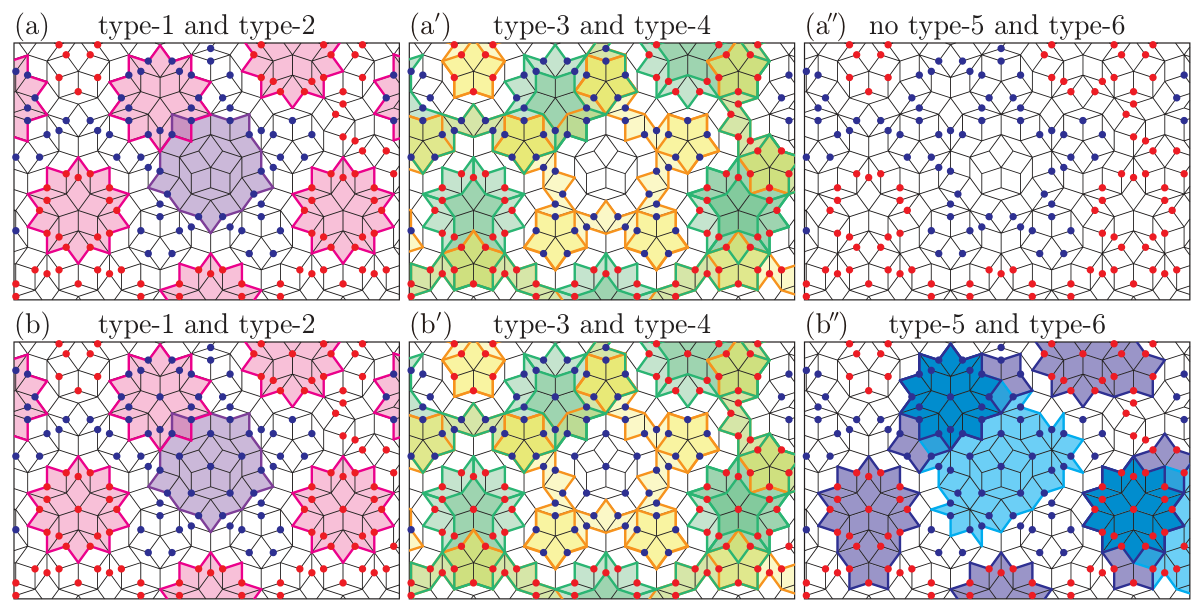
In contrast, the type-5 and type-6 building blocks, which contain both $z=3$ and $z=5$ sites with nonzero wavefunction amplitudes are eigenvectors of $\mathbf{T}$ but not of $\mathbf{M}$. Thus, the confined states at ${\epsilon }_k^{\mp }=3JS$ in the LSW Hamiltonian are linear combinations of type-1 to type-4 building blocks, whereas those at ${\epsilon }_k=0$ in the tight-binding Hamiltonian are linear combinations of type-1 to type-6 building blocks. Examples of the coverings of the Penrose lattice by these building blocks are shown in Figure A5.

4. Boundary-Condition Effects

The fractions of type-n building blocks in the thermodynamic limit, $f_n\equiv {lim}_{L\to \infty }{N}_n/L$, can be determined exactly using either the inflation-deflation rule [29,62] or the perpendicular-space accounting method [32]. These two independent methods conclude the same results. The values of $f_n$ are summarized in Table 2. The total fraction of confined states is given by ${\sum }_{n=1}^4{f}_n=280-173\tau \simeq 8.012\times {10}^{-2}$ for the LSW confined states at ${\epsilon }_k^{\mp }=3JS$, and by ${\sum }_{n=1}^6{f}_n=81-50\tau \simeq 9.830\times {10}^{-2}$ for the tight-binding confined states at ${\epsilon }_k=0$, where $\tau \equiv {\displaystyle \frac{1+\sqrt{5}}{2}}$ is the golden number.

Table 2. The fraction of each building block.

Building Blocks	Their Fraction
Type-1	$f_1={\displaystyle \frac{1}{{\tau }^8(1+{\tau }^2)}}\simeq 5.883\times {10}^{-3}$
Type-2	$f_2={\displaystyle \frac{1}{{\tau }^6(1+{\tau }^2)}}\simeq 1.540\times {10}^{-2}$
Type-3	$f_3={\displaystyle \frac{2}{{\tau }^8}}\simeq 4.257\times {10}^{-2}$
Type-4	$f_4={\displaystyle \frac{2}{{\tau }^{10}}}\simeq 1.626\times {10}^{-2}$
Type-5	$f_5={\displaystyle \frac{1}{{\tau }^9}}\simeq 1.316\times {10}^{-2}$
Type-6	$f_6={\displaystyle \frac{1}{{\tau }^{11}}}\simeq 5.025\times {10}^{-3}$
Total (LSW)	${\displaystyle \sum _{n=1}^4}{f}_n=280-173\tau \simeq 8.012\times {10}^{-2}$
Total (tight-binding)	${\displaystyle \sum _{n=1}^6}{f}_n=81-50\tau \simeq 9.830\times {10}^{-2}$

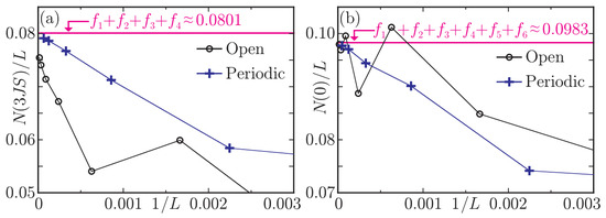
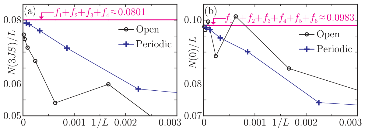
Let $N(\hslash \omega )$ denote the number of states with energy $\hslash \omega$. Figure 5 shows the finite-size scaling of the fractions $N\left(3JS\right)/L$ and $N\left(0\right)/L$ obtained numerically, corresponding to the ${\epsilon }_k^{\mp }=3JS$ eigenstates of the LSW Hamiltonian and ${\epsilon }_k=0$ eigenstates of the tight-binding Hamiltonian, respectively. For finite L, the fraction of confined states deviates from its thermodynamic-limit value. Since the wavefunctions of the confined states are strictly localized within the finite-extent building blocks shown in Figure 4, the Penrose lattice must be sufficiently large to accommodate a proper tiling by these building blocks. In the thermodynamic limit, the fraction of LSW ${\epsilon }_k^{\mp }=3JS$ confined states $N\left(3JS\right)/L$ converges to the estimated value $280-173\tau$ in boundary-free periodic approximants, but remains approximately $6\%$ lower even at L = 65,751 in an open-boundary cluster, as is shown in Figure 5a. In contrast, as shown in Figure 5b, the fraction of tight-binding ${\epsilon }_k=0$ confined states $N\left(0\right)/L$ converges to the exact value $81-50\tau$ regardless of the boundary conditions.

Figure 5. Finite-size scaling of the fraction of confined states at ${\epsilon }_k^{\mp }=3JS$ for the LSW Hamiltonian (a) and at ${\epsilon }_k=0$ for the tight-binding Hamiltonian (b), plotted as a function of $1/L$. Black circles represent results for open-boundary clusters, while blue crosses correspond to boundary-free periodic approximants. Magenta lines denote the analytically estimated fractions in the thermodynamic limit: ${\sum }_{n=1}^4{f}_n=280-173\tau$ for the LSW Hamiltonian and ${\sum }_{n=1}^6{f}_n=81-50\tau$ for the tight-binding Hamiltonian.

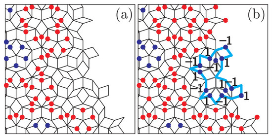
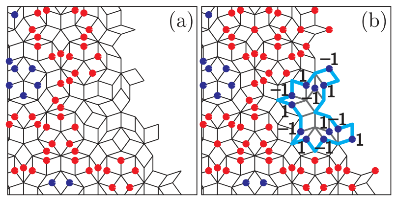
Figure 6 illustrates the effects of open boundaries. For the LSW confined states, blank domains without local solutions emerge near the boundaries, as shown in Figure 6a. This arises because the coordination number $z_l$ at boundary sites is reduced compared to the bulk, making it virtually impossible to simultaneously satisfy both the constraint that the wavefunction amplitude is nonzero only on tricoordinated sites and either Equation (15) or (16). As a result, ribbon-like blank domains, approximately one building block wide, form along the boundary and lead to an underestimation of $N\left(3JS\right)/L$ relative to the exact value. The fraction of such blank domains is estimated to be $O(1/\sqrt{L})$ in an L-site system, which is consistent in order of magnitude with the observed discrepancy in $N\left(3JS\right)/L$. In contrast, in boundary-free periodic approximants, the coordination numbers remain unaffected, thus preventing the formation of such blank domains. Consequently, the fraction $N\left(3JS\right)/L$ converges to the exact value $280-173\tau$, demonstrating that only type-1 to type-4 building blocks constitute the LSW confined states. In the case of the tight-binding Hamiltonian, i.e., the matrix $\mathbf{T}$, some of the ${\epsilon }_k=0$ eigenstates include building blocks other than types 1 to 6 as is shown in Figure 6b. As a result, the entire Penrose lattice can be covered, excluding the one-dimensional forbidden ladders, and $N\left(0\right)/L$ converges to the exact value $81-50\tau$ under both boundary conditions.

Figure 6. Effects of system boundaries on the confined states. Partial views of the confined states at ${\epsilon }_k^{\mp }=3JS$ for the LSW Hamiltonian (a) and at ${\epsilon }_k=0$ for the tight-binding Hamiltonian (b) on the Penrose lattice with $L=1591$ sites. Each vertex is marked in the same manner as in Figure 3. The region outlined in light blue in (b) does not correspond to any of the type-1 to type-6 building blocks, yet satisfies constraint (A12). The number adjacent to each dot indicates the relative amplitude of the unnormalized wavefunction.

Boundary-induced reduction of $N\left(3JS\right)$ may likewise occur in other quasiperiodic systems with confined states constructed from particular local building blocks, each consisting of same-coordinated sites. We evaluate the fraction of confined states for several open clusters of various sizes, which effectively correspond to different boundary terminations. The calculated fraction converges to the analytically derived value for the infinite-size lattice. This suggests that changing the boundary termination does not qualitatively alter the formation of finite-width blank domains near the boundaries. In addition, matching-rule-violating defect sites (see Appendix A.2 and Figure A3) emerge in periodic approximants of the Penrose lattice and locally obstruct the placement of the building blocks. As a result, point-like blank domains are formed around such defect sites, whereas boundary effects produce one-dimensional blank domains. The affected fractions therefore scale as $O(1/L)$ and $O(1/\sqrt{L})$, respectively. Owing to the local building-block nature of the LSW confined states on the Penrose lattice, the effects of boundaries, defects, and local disorder on the bulk confined-state fraction are expected to vanish in the thermodynamic limit.

5. Superconfined Antiferromagnons

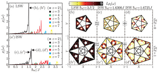
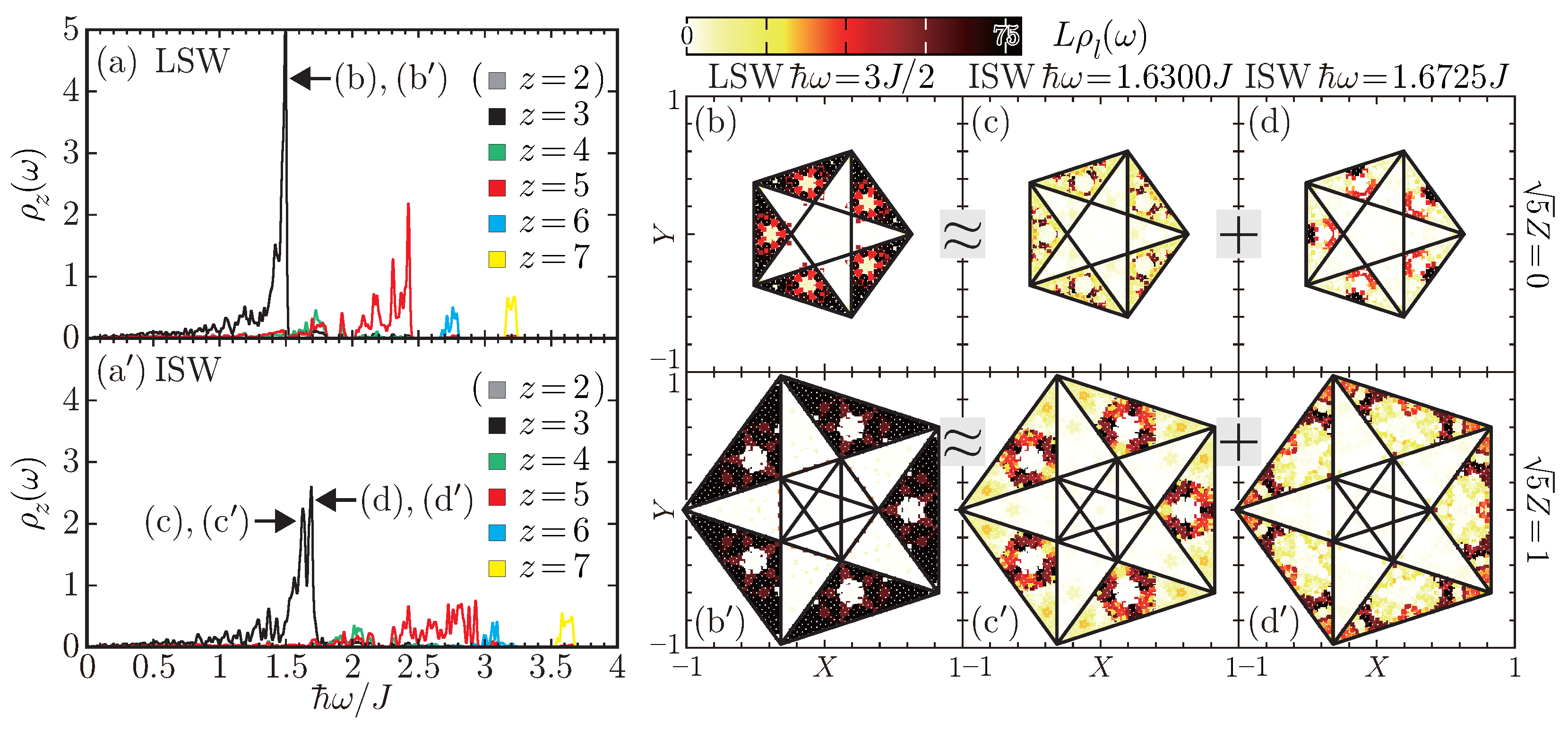
We incorporate the $O\left(S^0\right)$ quantum corrections (see Appendix C) into the LSW Hamiltonian via the Wick decomposition [63,64]. Figure 7 compares the site-resolved density of states for the LSW and up-to-$O\left(S^0\right)$ interacting spin-wave (ISW) excitation spectra at $S={\displaystyle \frac{1}{2}}$, together with their mappings in the perpendicular space. In the LSW spectrum, a prominent peak at $\hslash \omega =3J/2$ corresponds to massively degenerate confined states (Figure 7a). The $O\left(S^0\right)$ magnon-magnon interactions introduce environment-dependent corrections into the ISW Hamiltonian (A19). In the absence of translational invariance, interaction-induced on-site potentials vary even among sites with the same coordination number [56]. As a result, the $O\left(S^0\right)$ quantum corrections not only shift the excitation spectrum upward but also lift the degeneracy at $\hslash \omega =3J/2$. The corresponding peaks remain prominent in the ISW spectrum, but split into two peaks around $1.6300J$ and $1.6725J$ (Figure 7a′).

Figure 7. (Left panels) The coordination-number-resolved density of states ${\rho }_z\left(\omega \right)$ for the LSW (a) and ISW (a′) excitation spectra of the $S={\displaystyle \frac{1}{2}}$ Heisenberg model on the Penrose lattice of L = 11,006. Arrows in (a,a′) indicate the energies at which the perpendicular-space analyses of the site-resolved density of states are conducted. (Right panels) Contour plots in the perpendicular space of the site-resolved density of states ${\rho }_l\left(\omega \right)$ multiplied by the number of sites L for the LSW spectrum at $\hslash \omega =3J/2$ (b,b′), and for the ISW spectrum at $\hslash \omega =1.6300J$ (c,c′) and $\hslash \omega =1.6725J$ (d,d′). While results for $\sqrt{5}Z=0$ and $\sqrt{5}Z=1$ are presented here, the corresponding results for $\sqrt{5}Z=3$ and $\sqrt{5}Z=2$ are equivalent, respectively.

The one-to-one correspondence between positions in the perpendicular space and local vertices in the physical space (Figure A2) confirms that the LSW spectral weight at $\hslash \omega =3J/2$ (Figure 7b,b′) is localized within the $z=3$ domains. In these domains, certain regions exhibit negligible spectral intensity, consistent with the perpendicular-space analysis of forbidden regions [32] associated with the type-1 to type-4 building blocks. The perpendicular-space mappings of the ISW spectrum reveal that the spectral weight remains concentrated in the $z=3$ domains for both the lower branch at $\hslash \omega =1.6300J$ (Figure 7c,c′) and the upper branch at $\hslash \omega =1.6725J$ (Figure 7d,d′). Compared to the LSW case, however, the intensity exhibits a more fragmented distribution, with each branch occupying distinct subdomains. The subdivision of the perpendicular-space domains reflects a finer classification of local environments in the physical space, arising from the inclusion of more distant surrounding geometry [56,65]. The ISW spectral weight distributions of the two branches are complementary within the $z=3$ domains. This indicates that the $O\left(S^0\right)$ quantum fluctuations distinguish these subtle geometric variations and resolve subsets of tricoordinated sites into distinct energy branches. The magnons forming these two branches remain well confined to tricoordinated sites and are thus “superconfined” to selected subsets of these sites.

6. Summary and Discussion

In the vertex model on the Penrose lattice, itinerant electrons exhibit macroscopically degenerate confined states at ${\epsilon }_k=0$. They consist of type-1 to type-6 building blocks. In contrast, in the antiferromagnetic Heisenberg model on the Penrose lattice, localized spins exhibit macroscopically degenerate confined states at ${\epsilon }_k^{\mp }=3JS$ within the harmonic-oscillator approximation. They consist only of type-1 to type-4 building blocks. The spin-wave Hamiltonian in the site representation has coordination-number-dependent positive on-site potentials, which more stabilize lower-coordinated sites. Type-1 to type-4 building blocks consist of tricoordinated sites only, while type-5 and type-6 building blocks consist of pentacoordinated as well as tricoordinated sites. Confined spin waves consist purely of tricoordinated sites.

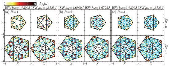
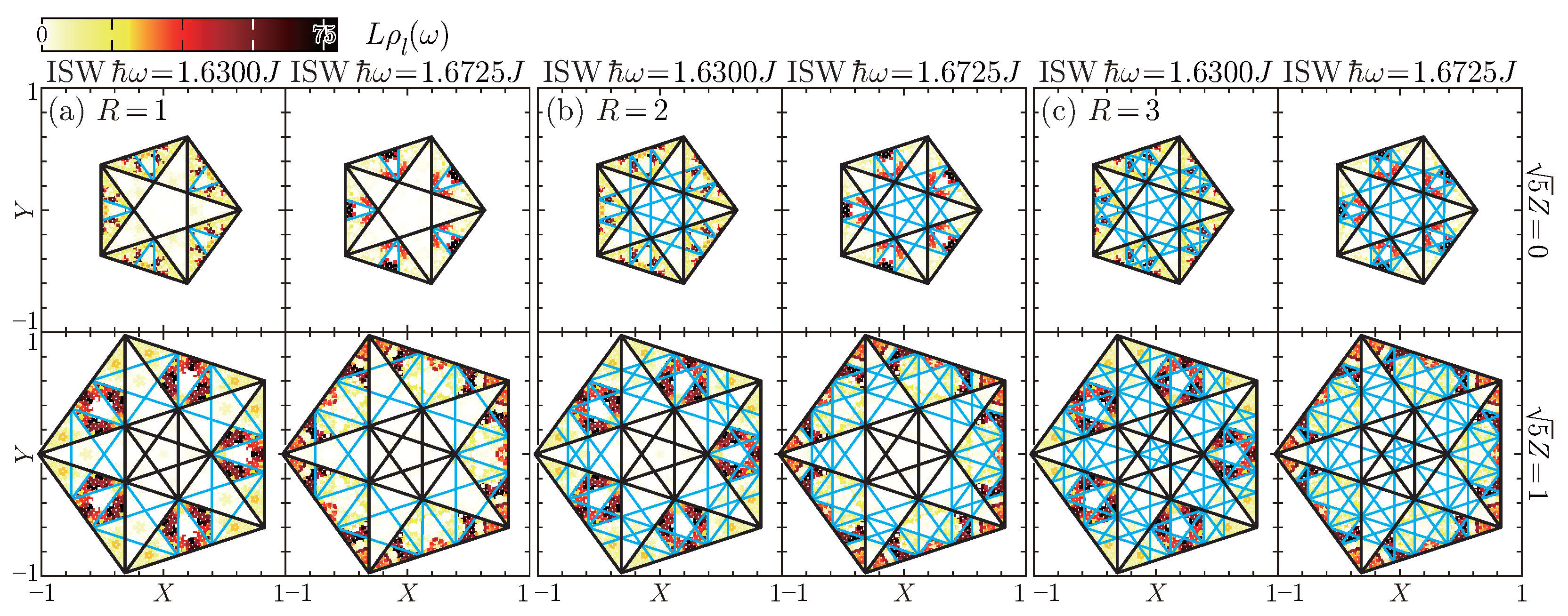
What will happen to confined antiferromagnons when they are brought into interaction? The $O\left(S^0\right)$ quartic interactions lift the macroscopic degeneracy at ${\epsilon }_k^{\mp }=3JS$ to yield two branches, as is shown in Figure 7. Their spectral weights are distributed complementarily in the perpendicular space. In order to formulate these distributions, we define a distance R between two vertices such that the shortest route from one to the other consists of R bonds. With increasing R, vertices are more and more classified into subgroups and subdomains in the physical and perpendicular spaces, respectively. The eight fundamental domains are further subdivided into 15, 27, and 40 types for $R=1$, 2, and 3, respectively. Overlaying these subdivisions onto the perpendicular-space distributions for each branch shows that the spectral-weight patterns are well described at $R=3$ (Figure 8). This can be understood as follows. As an example, consider an arbitrary bond $⟨i,j⟩$. In the LSW Hamiltonian, the matrix elements consist of on-site potentials determined by the coordination number of each site and uniform nearest-neighbor bonds. Thus, the LSW description is strictly local to each bond. In the ISW Hamiltonian, the $O\left(S^0\right)$ corrections to the quadratic terms contain site expectation values $⟨a_i^{†}{a}_i⟩$ and $⟨b_j^{†}{b}_j⟩$, and bond expectation values $⟨a_i{b}_j⟩$ and $⟨a_i^{†}{b}_j^{†}⟩$, as is shown in Equation (A16) (see Appendix C). These quantities depend on their local environments and therefore vary from bond to bond. They are self-consistently determined via matrix elements depending on the surrounding environments of each bond. Thus, the ISW description includes contributions beyond the bond in issue. Specifically, for the sites ${\mathit{r}}_i$ and ${\mathit{r}}_j(={\mathit{r}}_i+\mathit{\delta })$, the neighboring sites ${\mathit{r}}_{j^{\prime }}={\mathit{r}}_i+{\mathit{\delta }}_i$ ($\ne {\mathit{r}}_j$) and ${\mathit{r}}_{i^{\prime }}={\mathit{r}}_j+{\mathit{\delta }}_j$ ($\ne {\mathit{r}}_i$) also explicitly enter the ISW Hamiltonian. These sites are related by ${\mathit{r}}_{i^{\prime }}={\mathit{r}}_{j^{\prime }}-{\mathit{\delta }}_i+\mathit{\delta }+{\mathit{\delta }}_j$, implying that contributions up to a distance $R=3$ are relevant at the $O\left(S^0\right)$ level. This estimate is consistent with the spectral-weight distributions of the superconfined antiferromagnons.

Figure 8. Contour plots of the site-resolved density of states $L{\rho }_l\left(\omega \right)$ in the perpendicular space for the ISW spectrum at $\hslash \omega =1.6300J$ and $1.6725J$, overlaid with lines indicating the subdivision of the perpendicular-space domains. The domains are subdivided according to their surrounding environments in the physical space, defined by all vertices within a distance R from each vertex. Initially corresponding to the 8 types of vertices of the Penrose lattice (black lines), these domains are further subdivided into 15, 27, and 40 types for $R=1$ (a), $R=2$ (b), and $R=3$ (c), respectively (cyan lines).

What will happen to superconfined antiferromagnons when they are brought into further interactions higher than $O\left(S^0\right)$? The $O\left(S^{-1}\right)$ sextic interactions and still higher-order terms introduce additional corrections to the eigenvalues. Since the nearest-neighbor exchange interaction conserves magnetization, the expectation values in the quadratic terms obtained via Wick decomposition remain limited to the same types as in the $O\left(S^0\right)$ case: site expectation values $⟨a_i^{†}{a}_i⟩$ and $⟨b_j^{†}{b}_j⟩$, and bond expectation values $⟨a_i{b}_j⟩$ and $⟨a_i^{†}{b}_j^{†}⟩$. These expectation values are defined only on sites and nearest-neighbor bonds. The spatial range of the corrections remains unchanged from the $O\left(S^0\right)$ case. Thus, such higher-order corrections are unlikely to incorporate more distant environments to induce further branching. Superconfinement is not fractionalization up to infinity but dividing tricoordinated sites into essentially two groups.

Resonant inelastic x-ray scattering (RIXS) [66,67,68] may be a functional light probe to capture confined antiferromagnons of our interest. While spin-orbit-coupling-assisted magnetic Raman scattering [69,70] serves to reveal single magnon eigenlevels, the Raman operator of this type reads a total uniform magnetization in the polarization-dependent particular direction, and therefore acts only on rotation-invariant and mirror-symmetric magnons. It is thus useless to detect confined antiferromagnons consisting of mirror-antisymmetric building blocks. The single-magnon Raman scattering is further disappointing because it cannot have any access to the $\mathrm{SU}\left(2\right)$ symmetric Heisenberg Hamiltonian commutable with the total uniform magnetization in every direction. Inelastic neutron scattering [56,71] is indeed available in this context, but it requires relatively large bulk samples. RIXS works even with small samples and thin films. We can tune the momentum, polarization, and resonance energy of incoming and outgoing x-rays. Interestingly enough, photons can distinguish between sublattices. Circularly polarized light interacts with either a magnetization-enhancing or magnetization-reducing magnon. Each confined state resides in either the A or B sublattice, because its building blocks belong to either the A or B sublattice. There is a possibility of selectively accessing confined antiferromagnons according to their constituent building blocks. RIXS spectra possibly contain a nearly flat band at ${\epsilon }_k^{\mp }\simeq 3JS$.

Appendix A.1. Geometric Properties

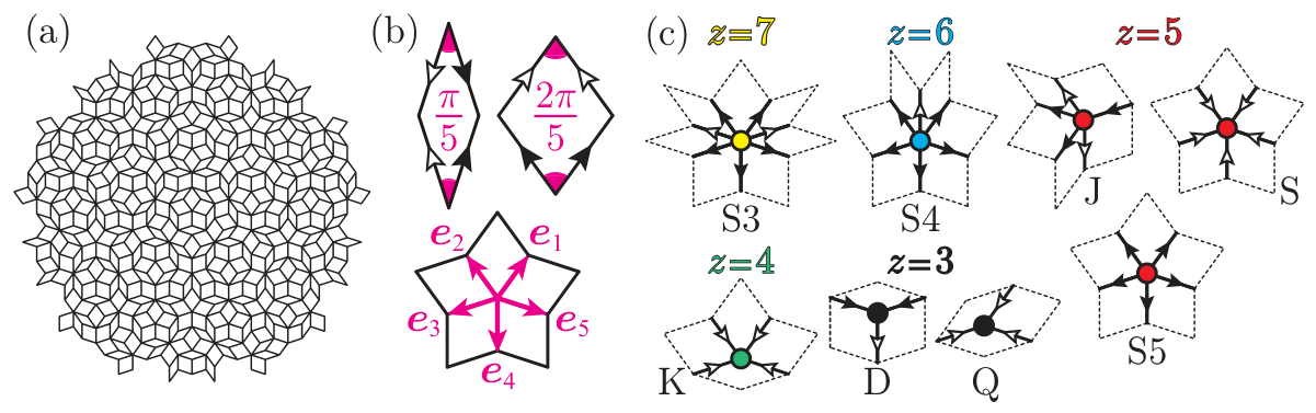
A two-dimensional Penrose lattice (Figure A1a) can be generated from two types of rhombuses with acute angles of ${\displaystyle \frac{\pi }{5}}$ and ${\displaystyle \frac{2\pi }{5}}$ (Figure A1b) by matching edges with identical arrow markings and iteratively applying the inflation-deflation operation [62,72]. These operations yield self-similarity with a magnification ratio equal to the golden number $\tau ={\displaystyle \frac{1+\sqrt{5}}{2}}$ [73]. Although the Penrose lattice has a crystallographically forbidden fivefold rotational symmetry, its diffraction pattern consists of sharp $\delta$-function peaks [74] and exhibits long-range positional order. While the physical space dimension d of the Penrose lattice is 2, its indexing dimension (or simply rank) D is 4. Every vertex of the Penrose lattice is represented by an integer linear combination of four independent primitive lattice vectors (Figure A1b). The Penrose lattice is bipartite, consisting of two sublattices, which we refer to as A and B. In general, a d-dimensional quasiperiodic lattice can be obtained from a higher-than-d-dimensional periodic lattice via an algebraic approach [75,76]. Both the Penrose lattice and its periodic approximants can be obtained as the projection of a five-dimensional hypercubic lattice onto a two-dimensional physical space (see Appendix A.2). The infinite Penrose lattice consists of eight types of local vertices whose coordination numbers z range from 3 to 7, as is shown in Figure A1c [75].

Figure A1. (a) A two-dimensional Penrose lattice of size $L=526$ with fivefold rotational symmetry. (b) The Penrose lattice consists of two rhombuses with acute angles ${\displaystyle \frac{\pi }{5}}$ and ${\displaystyle \frac{2\pi }{5}}$, respectively. Each edge is marked with an arrow to define the matching rules. The canonical basis vectors of a five-dimensional hypercubic lattice are projected onto five vectors, denoted by ${\mathit{e}}_1$, ${\mathit{e}}_2$, ${\mathit{e}}_3$, ${\mathit{e}}_4$, and ${\mathit{e}}_5$. Any four of these vectors can be chosen as the primitive translation vectors for the two-dimensional Penrose lattice. Note that ${\sum }_{n=1}^5{\mathit{e}}_n=\mathbf{0}$. (c) Eight types of vertices in the Penrose lattice with coordination numbers z ranging from 3 to 7 [75].

Figure A1. (a) A two-dimensional Penrose lattice of size $L=526$ with fivefold rotational symmetry. (b) The Penrose lattice consists of two rhombuses with acute angles ${\displaystyle \frac{\pi }{5}}$ and ${\displaystyle \frac{2\pi }{5}}$, respectively. Each edge is marked with an arrow to define the matching rules. The canonical basis vectors of a five-dimensional hypercubic lattice are projected onto five vectors, denoted by ${\mathit{e}}_1$, ${\mathit{e}}_2$, ${\mathit{e}}_3$, ${\mathit{e}}_4$, and ${\mathit{e}}_5$. Any four of these vectors can be chosen as the primitive translation vectors for the two-dimensional Penrose lattice. Note that ${\sum }_{n=1}^5{\mathit{e}}_n=\mathbf{0}$. (c) Eight types of vertices in the Penrose lattice with coordination numbers z ranging from 3 to 7 [75].

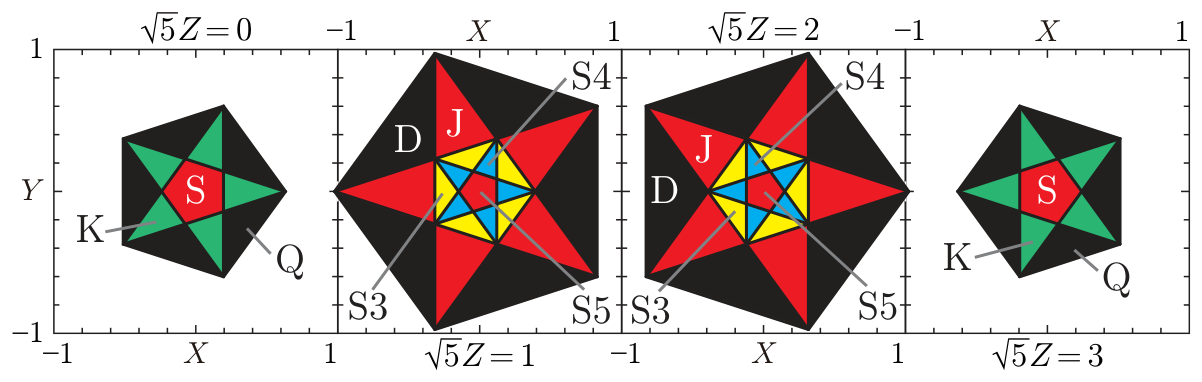
The orthogonal complement of the two-dimensional Penrose lattice is a three-dimensional stack of four pentagons (Figure A2). The layers at $\sqrt{5}Z=0,2$ correspond to the A sublattice, while those at $\sqrt{5}Z=1,3$ correspond to the B sublattice [cf. Equation (A2)]. Each of the eight vertex types maps onto a distinct compact region within the pentagons in the perpendicular space.

Figure A2. The perpendicular space of the Penrose lattice consists of a three-dimensional stack of four pentagons lying at $\sqrt{5}Z=0,1,2,3$. Each pentagon is divided into several color-coded domains, each of which contains a single species of vertices and is labeled with one of the eight types, D to S3, as is defined in Figure A1c.

Figure A2. The perpendicular space of the Penrose lattice consists of a three-dimensional stack of four pentagons lying at $\sqrt{5}Z=0,1,2,3$. Each pentagon is divided into several color-coded domains, each of which contains a single species of vertices and is labeled with one of the eight types, D to S3, as is defined in Figure A1c.

Appendix A.2. Projection Method and Periodic Approximants of the Penrose Lattice

The Penrose lattice is constructed by projecting a five-dimensional hypercubic lattice onto a two-dimensional physical space [53,57]. The projection matrix for the two-dimensional physical-space coordinates $(x,y)$ is

$$\begin{array}{cc}\hfill & \left[\begin{array}{c}x\\ y\end{array}\right]=\sqrt{{\displaystyle \frac{2}{5}}}\left[\begin{array}{ccccc}1& cos{\varphi }_1& cos{\varphi }_2& cos{\varphi }_3& cos{\varphi }_4\\ 0& sin{\varphi }_1& sin{\varphi }_2& sin{\varphi }_3& sin{\varphi }_4\end{array}\right]\left[\begin{array}{c}{m}_1\\ m_2\\ m_3\\ m_4\\ m_5\end{array}\right];{\varphi }_n\equiv {\displaystyle \frac{2\pi }{5}}n,m_n\in \mathbb{Z}.\hfill \end{array}$$

(A1)

The projection matrix for the three-dimensional perpendicular-space coordinates $(X,Y,Z)$ is

$$\begin{array}{c}\hfill \left[\begin{array}{c}X\\ Y\\ Z\end{array}\right]=\sqrt{{\displaystyle \frac{2}{5}}}\left[\begin{array}{ccccc}1& c_2& c_4& c_6& c_8\\ 0& s_2& s_4& s_6& s_8\\ {\displaystyle \frac{1}{\sqrt{2}}}& {\displaystyle \frac{1}{\sqrt{2}}}& {\displaystyle \frac{1}{\sqrt{2}}}& {\displaystyle \frac{1}{\sqrt{2}}}& {\displaystyle \frac{1}{\sqrt{2}}}\end{array}\right]\left[\begin{array}{c}{m}_1\\ m_2\\ m_3\\ m_4\\ m_5\end{array}\right],\end{array}$$

(A2)

where $c_n=cos{\varphi }_n$ and $s_n=sin{\varphi }_n$ for the quasiperiodic Penrose lattice. Only the five-dimensional integer vectors ${}^t[m_1,m_2,m_3,m_4,m_5]$ whose projections onto the three-dimensional perpendicular space fall within a certain region, called the selection window, are retained as lattice points in the two-dimensional physical space. The selection window of the Penrose lattice is a rhombic icosahedron, which corresponds to the projection of a five-dimensional unit hypercube. Its cross-section, containing the selected lattice points, consists of a stack of four regular pentagons at positions where $\sqrt{5}Z\in \mathbb{Z}$, as is shown in Figure A2.

In order to construct periodic approximants, $c_n$ and $s_n$ in Equation (A2) are replaced by the following rational approximations:

$$\begin{array}{cc}\hfill & c_2=-{\displaystyle \frac{{\tau }_1}{2}},c_4={\displaystyle \frac{{\tau }_1-1}{2}},c_6={\displaystyle \frac{{\tau }_1-1}{2}},c_8=-{\displaystyle \frac{{\tau }_1}{2}},\hfill \\ \hfill & s_2={\tau }_2-1,s_4={\tau }_3-{\tau }_2-1,s_6=1,s_8=1-{\tau }_2,\hfill \end{array}$$

(A3)

where

$$\begin{array}{cc}\hfill & {\tau }_1={\displaystyle \frac{F_{i+2}+F_i}{F_{i+1}+F_{i-1}}},{\tau }_2=1+{\displaystyle \frac{F_{i+1}(F_i+F_{i-2})}{F_{i-1}(F_{i+3}+F_{i+1})}},{\tau }_3={\displaystyle \frac{F_{i+4}+F_{i+2}}{F_{i+3}+F_{i+1}}}\hfill \end{array}$$

(A4)

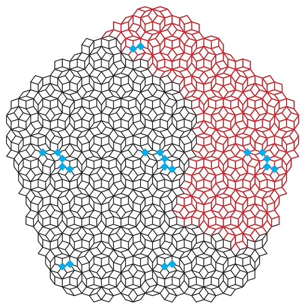
and $F_i$ denotes the Fibonacci numbers defined by the recurrence relation $F_0=0,$$F_1=1,$$F_i=F_{i-1}+F_{i-2}(i\ge 2)$ [31]. This procedure yields a periodic unit cell in the two-dimensional physical space that reproduces the local environments of the Penrose lattice at the majority of vertices, as is illustrated in Figure A3. Vertices sharing identical coordinates in the three-dimensional perpendicular space are connected by translation operations in the two-dimensional physical space.

Figure A3. Physical-space projection for $-7\le m_n\le 7$ using the periodic approximant projection matrix with Fibonacci index $i=5$ (black), along with corresponding periodic unit cell consisting of $L=445$ sites (red). Light blue diamonds indicate vertices that violate the local environments of the Penrose lattice depicted in Figure A1c.

Figure A3. Physical-space projection for $-7\le m_n\le 7$ using the periodic approximant projection matrix with Fibonacci index $i=5$ (black), along with corresponding periodic unit cell consisting of $L=445$ sites (red). Light blue diamonds indicate vertices that violate the local environments of the Penrose lattice depicted in Figure A1c.

Appendix B.1. Tight-Binding Hamiltonian

We define the tight-binding Hamiltonian on the two-dimensional Penrose lattice with $L=L_{\mathrm{A}}+L_{\mathrm{B}}$ sites

$$\begin{array}{cc}\hfill & {\mathcal{H}}_t=-t\sum _{i\in \mathrm{A}}\sum _{j\in \mathrm{B}}{l}_{i,j}\left(c_i^{†}{c}_j+c_j^{†}{c}_i\right)\equiv -t{\mathit{c}}^{†}\mathbf{T}\mathit{c}\equiv -t\left[{\mathit{c}}_{\mathrm{A}}^{†},{\mathit{c}}_{\mathrm{B}}^{†}\right]\left[\begin{array}{cc}{\mathbf{O}}_{\mathrm{AA}}& {\mathbf{C}}_{\mathrm{AB}}\\ {\mathbf{C}}_{\mathrm{AB}}^{†}& {\mathbf{O}}_{\mathrm{BB}}\end{array}\right]\left[\begin{array}{c}{\mathit{c}}_{\mathrm{A}}\\ {\mathit{c}}_{\mathrm{B}}\end{array}\right];\hfill \\ \hfill & {\mathit{c}}_{\mathrm{A}}^{†}=\left[c_1^{†},\dots ,c_{L_{\mathrm{A}}}^{†}\right],{\mathit{c}}_{\mathrm{B}}^{†}=\left[c_{L_{\mathrm{A}}+1}^{†},\dots ,c_{L_{\mathrm{A}}+L_{\mathrm{B}}}^{†}\right],{\left[{\mathbf{O}}_{\mathrm{AA}}\right]}_{i,i^{\prime }}={\left[{\mathbf{O}}_{\mathrm{BB}}\right]}_{j,j^{\prime }}=0,{\left[{\mathbf{C}}_{\mathrm{AB}}\right]}_{i,j}=l_{i,j},\hfill \end{array}$$

(A5)

where the site indices are labeled as $i\in \mathrm{A}$ and $j\in \mathrm{B}$. We denote a generic site—meaning one that may belong to either the A or B sublattice—by ${\mathit{r}}_l$, and let $c_l^{†}$ denote the creation operator of an electron at site ${\mathit{r}}_l$. Note that we omit the spin degrees of freedom of the electrons, as they do not affect the present discussion. ${\mathit{c}}^{†}$, ${\mathit{c}}_{\mathrm{A}}^{†}$, and ${\mathit{c}}_{\mathrm{B}}^{†}$ are row vectors of dimension L, $L_{\mathrm{A}}$, and $L_{\mathrm{B}}$, respectively. ${\mathbf{O}}_{\mathrm{AA}}$ and ${\mathbf{O}}_{\mathrm{BB}}$ are zero matrices of dimension $L_{\mathrm{A}}\times L_{\mathrm{A}}$ and $L_{\mathrm{B}}\times L_{\mathrm{B}}$, respectively, and ${\mathbf{C}}_{\mathrm{AB}}$ is the biadjacency matrix of dimension $L_{\mathrm{A}}\times L_{\mathrm{B}}$. The linkage identifier $l_{i,j}$ equals 1 if the vertices ${\mathit{r}}_i$ and ${\mathit{r}}_j$ are connected, and 0 otherwise. t denotes the transfer integral for electron hopping. Applying a standard unitary transformation

$$\begin{array}{c}\hfill \left[\begin{array}{c}{\mathit{c}}_{\mathrm{A}}\\ {\mathit{c}}_{\mathrm{B}}\end{array}\right]=\mathbf{U}\mathit{\alpha };{\left[\mathbf{U}\right]}_{l,k}\equiv u_{l,k},{\mathit{\alpha }}^{†}\equiv \left[{\alpha }_1^{†},\dots ,{\alpha }_L^{†}\right]\end{array}$$

(A6)

diagonalizes the Hamiltonian (A5) as

$$\begin{array}{c}\hfill {\mathcal{H}}_t={\displaystyle \sum _{k=1}^L}{\epsilon }_k{\alpha }_k^{†}{\alpha }_k,\end{array}$$

(A7)

where ${\alpha }_k^{†}$ creates a quasiparticle fermion of energy ${\epsilon }_k$.

We define the site-resolved density of states for the quasiparticle fermion excitation spectrum

$$\begin{array}{cc}\hfill & \rho \left(\omega \right)={\displaystyle \sum _{l=1}^L}{\rho }_l\left(\omega \right)={\displaystyle \sum _{z=3}^7}{\rho }_z\left(\omega \right)={\displaystyle \sum _{z=3}^7}{\displaystyle \frac{1}{L}}{\displaystyle \sum _{k=1}^L}{\displaystyle \frac{{\sum }_{l(z_l=z)}{\left|u_{l,k}\right|}^2}{{\sum }_{l=1}^L{\left|u_{l,k}\right|}^2}}\delta \left(\hslash \omega -{\epsilon }_k\right),\hfill \end{array}$$

(A8)

where $z_l$ is the coordination number of the vertex at ${\mathit{r}}_l$. Figure A4 shows the coordination-number-resolved density of states for the tight-binding excitation spectrum (A8). The density of states is highly singular, exhibiting spikes across all energies. We find that the $\delta$-function peak at $\hslash \omega =0$ accounts for approximately 10% of the total number of states, which implies the existence of confined states. This peak is separated from the rest of the spectrum—two symmetric continua—by a gap of about $0.17t$ [29,34]. The $\delta$-function peak is essentially composed of tricoordinated and pentacoordinated sites, whereas the remaining states have nonzero weights for all coordination numbers.

Figure A4. The coordination-number-resolved density of states ${\rho }_z\left(\omega \right)$ for the tight-binding excitation spectrum on the Penrose lattice with L = 11,006, where z ranges from 3 to 7. Note that $z=2$ vertices are artifacts of finite open-boundary clusters.

Figure A4. The coordination-number-resolved density of states ${\rho }_z\left(\omega \right)$ for the tight-binding excitation spectrum on the Penrose lattice with L = 11,006, where z ranges from 3 to 7. Note that $z=2$ vertices are artifacts of finite open-boundary clusters.

Appendix B.2. Zero-Energy Confined States

We derive the constraints on the zero-energy eigenstates of the connectivity matrix $\mathbf{T}$. The eigenvector ${\mathit{u}}_k$ corresponding to eigenstate index k is given by

$$\begin{array}{cc}\hfill & {\mathit{u}}_k=\left[\begin{array}{c}{u}_{1,k}\\ ⋮\\ u_{L_{\mathrm{A}},k}\\ u_{L_{\mathrm{A}}+1,k}\\ ⋮\\ u_{L_{\mathrm{A}}+L_{\mathrm{B}},k}\end{array}\right]\equiv \left[\begin{array}{c}{\mathit{u}}_{\mathrm{A};k}\\ {\mathit{u}}_{\mathrm{B};k}\end{array}\right];{\left[{\mathit{u}}_{\mathrm{A};k}\right]}_i=u_{i,k},{\left[{\mathit{u}}_{\mathrm{B};k}\right]}_j=u_{L_{\mathrm{A}}+j,k}.\hfill \end{array}$$

(A9)

The eigenvector ${\mathit{u}}_k$ satisfies the eigenvalue equation

$$\begin{array}{c}\hfill \mathbf{T}{\mathit{u}}_k=-{\displaystyle \frac{{\epsilon }_k}{t}}{\mathit{u}}_k.\end{array}$$

(A10)

Since the connectivity matrix $\mathbf{T}$ is expressed in terms of the biadjacency matrix ${\mathbf{C}}_{\mathrm{AB}}$ as shown in Equation (9), the left-hand side of Equation (A10) can be written as

$$\begin{array}{cc}\hfill & \mathbf{T}{\mathit{u}}_k=\left[\begin{array}{c}{\mathbf{C}}_{\mathrm{AB}}{\mathit{u}}_{\mathrm{B};k}\\ {\mathbf{C}}_{\mathrm{AB}}^{†}{\mathit{u}}_{\mathrm{A};k}\end{array}\right];{\left[{\mathbf{C}}_{\mathrm{AB}}{\mathit{u}}_{\mathrm{B};k}\right]}_i=\sum _{j\in \mathrm{B}}{l}_{i,j}{u}_{L_{\mathrm{A}}+j,k},{\left[{\mathbf{C}}_{\mathrm{AB}}^{†}{\mathit{u}}_{\mathrm{A};k}\right]}_j=\sum _{i\in \mathrm{A}}{l}_{i,j}{u}_{i,k}.\hfill \end{array}$$

(A11)

Therefore, for ${\epsilon }_k=0$, the wavefunction amplitudes must satisfy

$$\begin{array}{c}\hfill \left\{\begin{array}{cc}{\displaystyle \sum _{j\in \mathrm{B}}}{l}_{i,j}{u}_{L_{\mathrm{A}}+j,k}=0\hfill & (l=i\in \mathrm{A})\hfill \\ {\displaystyle \sum _{i\in \mathrm{A}}}{l}_{i,j}{u}_{i,k}=0\hfill & (l=j\in \mathrm{B})\hfill \end{array}\right..\end{array}$$

(A12)

The confined states of the Penrose lattice are divided into discrete domains by the forbidden ladders (Figure 3), which allows each domain to be treated independently. Within each domain, the confined states have finite amplitudes on only one of the two sublattices, A or B. Let us consider a domain in which the amplitudes are finite only on the A-sublattice. The analogous argument applies to domains with finite amplitudes only on the B-sublattice. Equation (A12) is automatically satisfied for all A-sublattice sites ${\mathit{r}}_i$, since $u_{L_{\mathrm{A}}+j,k}=0$ for all adjacent B-sublattice sites ${\mathit{r}}_j$. In contrast, for B-sublattice sites within the same domain, Equation (A12) must be satisfied explicitly, since $u_{i,k}$ may be nonzero. There are exactly six types of local solutions satisfying these constraints in the infinite Penrose lattice, as is shown in Figure 4 [28,29,34]. The ${\epsilon }_k=0$ eigenstates of the tight-binding Hamiltonian are linear combinations of type-1 to type-6 building blocks on the Penrose lattice.

Appendix B.3. Coverings of the Penrose Lattice Using the Building Blocks of Confined States

We demonstrate that linear combinations of the building blocks constitute the confined states. As an example, we focus on the rectangular regions highlighted in Figure 3. Figure A5 illustrates how the Penrose lattice is covered by specific building blocks of the confined states at ${\epsilon }_k^{\mp }=3JS$ in the linear spin-wave (LSW) Hamiltonian (13) and at ${\epsilon }_k=0$ in the tight-binding Hamiltonian (A7). The ${\epsilon }_k^{\mp }=3JS$ confined states in the LSW Hamiltonian are covered by type-1 to type-4 building blocks (excluding type-5 and type-6), whereas the ${\epsilon }_k=0$ confined states in the tight-binding Hamiltonian are covered by all six types.

Figure A5. Enlarged views of the rectangular regions highlighted in Figure 3. The ${\epsilon }_k^{\mp }=3JS$ eigenstates of the LSW Hamiltonian [(a–a″)] and ${\epsilon }_k=0$ eigenstates of the tight-binding Hamiltonian [(b–b″)]. Color-coded regions indicate the building blocks of each confined state (magenta: type-1, purple: type-2, yellow: type-3, green: type-4, blue: type-5, and light blue: type-6). The actual confined states at ${\epsilon }_k^{\mp }=3JS$ and ${\epsilon }_k=0$ are superpositions of the patterns shown in panels (a–a″) and (b–b″), respectively.

Figure A5. Enlarged views of the rectangular regions highlighted in Figure 3. The ${\epsilon }_k^{\mp }=3JS$ eigenstates of the LSW Hamiltonian [(a–a″)] and ${\epsilon }_k=0$ eigenstates of the tight-binding Hamiltonian [(b–b″)]. Color-coded regions indicate the building blocks of each confined state (magenta: type-1, purple: type-2, yellow: type-3, green: type-4, blue: type-5, and light blue: type-6). The actual confined states at ${\epsilon }_k^{\mp }=3JS$ and ${\epsilon }_k=0$ are superpositions of the patterns shown in panels (a–a″) and (b–b″), respectively.

References

- Levine, D.; Steinhardt, P.J. Quasicrystals: A New Class of Ordered Structures. Phys. Rev. Lett. 1984, 53, 2477. [Google Scholar] [CrossRef] [Scilit]
- Levine, D.; Steinhardt, P.J. Quasicrystals. I. Definition and structure. Phys. Rev. B 1986, 34, 596. [Google Scholar] [CrossRef] [Scilit] [PubMed]
- Shechtman, D.; Blech, I.; Gratias, D.; Cahn, J.W. Metallic Phase with Long-Range Orientational Order and No Translational Symmetry. Phys. Rev. Lett. 1984, 53, 1951. [Google Scholar] [CrossRef] [Scilit]
- Tsai, A.P.; Inoue, A.; Masumoto, T. A Stable Quasicrystal in Al-Cu-Fe System. Jpn. J. Appl. Phys. 1987, 26, L1505. [Google Scholar] [CrossRef] [Scilit]
- Tsai, A.P.; Inoue, A.; Masumoto, T. New Stable Icosahedral Al-Cu-Ru and Al-Cu-Os Alloys. Jpn. J. Appl. Phys. 1988, 27, L1587. [Google Scholar] [CrossRef] [Scilit]
- Tsai, A.P.; Inoue, A.; Yokoyama, Y.; Masumoto, T. Stable Icosahedral Al-Pd-Mn and Al-Pd-Re Alloys. Mater. Trans. JIM 1990, 31, 98. [Google Scholar] [CrossRef] [Scilit]
- Tsai, A.P.; Guo, J.Q.; Abe, E.; Takakura, H.; Sato, T.J. A stable binary quasicrystal. Nature 2000, 408, 537. [Google Scholar] [CrossRef] [Scilit]
- Tamura, R.; Ishikawa, A.; Suzuki, S.; Kotajima, T.; Tanaka, Y.; Seki, T.; Shibata, N.; Yamada, T.; Fujii, T.; Wang, C.-W.; et al. Experimental Observation of Long-Range Magnetic Order in Icosahedral Quasicrystals. J. Am. Chem. Soc. 2021, 143, 19938. [Google Scholar] [CrossRef] [Scilit]
- Takeuchi, R.; Labib, F.; Tsugawa, T.; Akai, Y.; Ishikawa, A.; Suzuki, S.; Fujii, T.; Tamura, R. High Phase-Purity and Composition-Tunable Ferromagnetic Icosahedral Quasicrystal. Phys. Rev. Lett. 2023, 130, 176701. [Google Scholar] [CrossRef] [Scilit]
- Tamura, R.; Abe, T.; Yoshida, S.; Shimozaki, Y.; Suzuki, S.; Ishikawa, A.; Labib, F.; Avdeev, M.; Kinjo, K.; Nawa, K.; et al. Observation of antiferromagnetic order in a quasicrystal. Nat. Phys. 2025, 21, 974. [Google Scholar] [CrossRef] [Scilit]
- Tamura, R.; Muro, Y.; Hiroto, T.; Nishimoto, K.; Takabatake, T. Long-range magnetic order in the quasicrystalline approximant Cd6Tb. Phys. Rev. B 2010, 82, 220201(R). [Google Scholar] [CrossRef] [Scilit]
- Ishikawa, A.; Hiroto, T.; Tokiwa, K.; Fujii, T.; Tamura, R. Composition-driven spin glass to ferromagnetic transition in the quasicrystal approximant Au-Al-Gd. Phys. Rev. B 2016, 93, 024416. [Google Scholar] [CrossRef] [Scilit]
- Ishikawa, A.; Fujii, T.; Takeuchi, T.; Yamada, T.; Matsushita, Y.; Tamura, R. Antiferromagnetic order is possible in ternary quasicrystal approximants. Phys. Rev. B 2018, 98, 220403(R). [Google Scholar] [CrossRef] [Scilit]
- Yoshida, S.; Suzuki, S.; Yamada, T.; Fujii, T.; Ishikawa, A.; Tamura, R. Antiferromagnetic order survives in the higher-order quasicrystal approximant. Phys. Rev. B 2019, 100, 180409(R). [Google Scholar]
- Sato, N.K.; Ishimasa, T.; Deguchi, K.; Imura, K. Effects of Electron Correlation and Geometrical Frustration on Magnetism of Icosahedral Quasicrystals and Approximants—An Attempt to Bridge the Gap between Quasicrystals and Heavy Fermions. J. Phys. Soc. Jpn. 2022, 91, 072001. [Google Scholar] [CrossRef] [Scilit]
- Deguchi, K.; Matsukawa, S.; Sato, N.K.; Hattori, T.; Ishida, K.; Takakura, H.; Ishimasa, T. Quantum critical state in a magnetic quasicrystal. Nat. Mater. 2012, 11, 1013. [Google Scholar] [CrossRef] [Scilit] [PubMed]
- Kamiya, K.; Takeuchi, T.; Kabeya, N.; Wada, N.; Ishimasa, T.; Ochiai, A.; Deguchi, K.; Imura, K.; Sato, N.K. Discovery of superconductivity in quasicrystal. Nat. Commun. 2018, 9, 154. [Google Scholar] [CrossRef] [Scilit]
- Watanabe, S.; Yamada, T.; Takakura, H.; Fujita, N. Monte Carlo study on critical exponents of the classical Heisenberg model in ferromagnetic icosahedral quasicrystal. Phys. Rev. Res. 2025, 7, 043113. [Google Scholar] [CrossRef] [Scilit]
- Sakai, S.; Takemori, N.; Koga, A.; Arita, R. Superconductivity on a quasiperiodic lattice: Extended-to-localized crossover of Cooper pairs. Phys. Rev. B 2017, 95, 024509. [Google Scholar] [CrossRef] [Scilit]
- Sakai, S.; Arita, R. Exotic pairing state in quasicrystalline superconductors under a magnetic field. Phys. Rev. Res. 2019, 1, 022002(R). [Google Scholar]
- Takemori, N.; Arita, R.; Sakai, S. Physical properties of weak-coupling quasiperiodic superconductors. Phys. Rev. B 2020, 102, 115108. [Google Scholar] [CrossRef] [Scilit]
- Duncan, C.W.; Manna, S.; Nielsen, A.E.B. Topological models in rotationally symmetric quasicrystals. Phys. Rev. B 2020, 101, 115413. [Google Scholar] [CrossRef] [Scilit]
- Ghadimi, R.; Sugimoto, T.; Tohyama, T. Higher-dimensional Hofstadter butterfly on the Penrose lattice. Phys. Rev. B 2022, 106, L201113. [Google Scholar] [CrossRef] [Scilit]
- Sakai, S.; Arita, R.; Ohtsuki, T. Hyperuniform electron distributions controlled by electron interactions in quasicrystals. Phys. Rev. B 2022, 105, 054202. [Google Scholar] [CrossRef] [Scilit]
- Penrose, R. The role of aesthetics in pure and applied mathematical research. Bull. Inst. Math. Appl. 1974, 10, 266. [Google Scholar]
- Choy, T.C. Density of States for a Two-Dimensional Penrose Lattice: Evidence of a Strong Van Hove Singularity. Phys. Rev. Lett. 1985, 55, 2915. [Google Scholar] [CrossRef] [Scilit]
- Odagaki, T.; Nguyen, D. Electronic and vibrational spectra of two-dimensional quasicrystals. Phys. Rev. B 1986, 33, 2184. [Google Scholar] [CrossRef] [Scilit]
- Kohmoto, M.; Sutherland, B. Electronic States on a Penrose Lattice. Phys. Rev. Lett. 1986, 56, 2740. [Google Scholar] [CrossRef] [Scilit]
- Arai, M.; Tokihiro, T.; Fujiwara, T.; Kohmoto, M. Strictly localized states on a two-dimensional Penrose lattice. Phys. Rev. B 1988, 38, 1621. [Google Scholar] [CrossRef] [Scilit]
- Rieth, T.; Schreiber, M. Identification of spatially confined states in two-dimensional quasiperiodic lattices. Phys. Rev. B 1995, 51, 15827. [Google Scholar] [CrossRef] [Scilit]
- Zijlstra, E.S.; Janssen, T. Density of states and localization of electrons in a tight-binding model on the Penrose tiling. Phys. Rev. B 2000, 61, 3377. [Google Scholar] [CrossRef] [Scilit]
- Mirzhalilov, M.; Oktel, M.Ö. Perpendicular space accounting of localized states in a quasicrystal. Phys. Rev. B 2020, 102, 064213. [Google Scholar] [CrossRef] [Scilit]
- Day-Roberts, E.; Fernandes, R.M.; Kamenev, A. Nature of protected zero-energy states in Penrose quasicrystals. Phys. Rev. B 2020, 102, 064210. [Google Scholar] [CrossRef] [Scilit]
- Koga, A.; Tsunetsugu, H. Antiferromagnetic order in the Hubbard model on the Penrose lattice. Phys. Rev. B 2017, 96, 214402. [Google Scholar] [CrossRef] [Scilit]
- Oktel, M.Ö. Localized states in local isomorphism classes of pentagonal quasicrystals. Phys. Rev. B 2022, 106, 024201. [Google Scholar] [CrossRef] [Scilit]
- Koga, A. Superlattice structure in the antiferromagnetically ordered state in the Hubbard model on the Ammann–Beenker tiling. Phys. Rev. B 2020, 102, 115125. [Google Scholar] [CrossRef] [Scilit]
- Oktel, M.Ö. Strictly localized states in the octagonal Ammann–Beenker quasicrystal. Phys. Rev. B 2021, 104, 014204. [Google Scholar] [CrossRef] [Scilit]
- Koga, A. Antiferromagnetically Ordered State in the Half-Filled Hubbard Model on the Socolar Dodecagonal Tiling. Mater. Trans. 2021, 62, 360. [Google Scholar] [CrossRef] [Scilit]
- Akif Keskiner, M.; Oktel, M.Ö. Strictly localized states on the Socolar dodecagonal lattice. Phys. Rev. B 2022, 106, 064207. [Google Scholar] [CrossRef] [Scilit]
- Koga, A.; Coates, S. Ferrimagnetically ordered states in the Hubbard model on the hexagonal golden-mean tiling. Phys. Rev. B 2022, 105, 104410. [Google Scholar] [CrossRef] [Scilit]
- Matsubara, T.; Koga, A.; Coates, S. Ferromagnetically ordered states in the Hubbard model on the H00 hexagonal golden-mean tiling. Phys. Rev. B 2024, 109, 014413. [Google Scholar] [CrossRef] [Scilit]
- Ha, H.; Yang, B.-J. Macroscopically degenerate localized zero-energy states of quasicrystalline bilayer systems in the strong coupling limit. Phys. Rev. B 2021, 104, 165112. [Google Scholar] [CrossRef] [Scilit]
- Schirmann, J.; Franca, S.; Flicker, F.; Grushin, A.G. Physical Properties of an Aperiodic Monotile with Graphene-like Features, Chirality, and Zero Modes. Phys. Rev. Lett. 2024, 132, 086402. [Google Scholar] [CrossRef] [Scilit] [PubMed]
- Tsunetsugu, H.; Fujiwara, T.; Ueda, K.; Tokihiro, T. Eigenstates in 2-Dimensional Penrose Tiling. J. Phys. Soc. Jpn. 1986, 55, 1420. [Google Scholar] [CrossRef] [Scilit]
- Fujiwara, T.; Arai, M.; Tokihiro, T.; Kohmoto, M. Localized states and self-similar states of electrons on a two-dimensional Penrose lattice. Phys. Rev. B 1988, 37, 2797. [Google Scholar] [CrossRef] [Scilit] [PubMed]
- Tsunetsugu, H.; Fujiwara, T.; Ueda, K.; Tokihiro, T. Electronic properties of the Penrose lattice. I. Energy spectrum and wave functions. Phys. Rev. B 1991, 43, 8879. [Google Scholar] [CrossRef] [Scilit]
- Ghadimi, R.; Hori, M.; Sugimoto, T.; Tohyama, T. Confined states and topological phases in two-dimensional quasicrystalline π-flux model. Phys. Rev. B 2023, 108, 125104. [Google Scholar] [CrossRef] [Scilit]
- Takahashi, M. Half-filled Hubbard model at low temperature. J. Phys. C 1977, 10, 1289. [Google Scholar] [CrossRef] [Scilit]
- MacDonald, A.H.; Girvin, S.M.; Yoshioka, D. tU expansion for the Hubbard model. Phys. Rev. B 1988, 37, 9753. [Google Scholar] [CrossRef] [Scilit]
- Jagannathan, A.; Szallas, A.; Wessel, S.; Duneau, M. Penrose quantum antiferromagnet. Phys. Rev. B 2007, 75, 212407. [Google Scholar] [CrossRef] [Scilit]
- Wessel, S.; Jagannathan, A.; Haas, S. Quantum Antiferromagnetism in Quasicrystals. Phys. Rev. Lett. 2003, 90, 177205. [Google Scholar] [CrossRef] [Scilit]
- Sandvik, A.W. Finite-size scaling of the ground-state parameters of the two-dimensional Heisenberg model. Phys. Rev. B 1997, 56, 11678. [Google Scholar] [CrossRef] [Scilit]
- Szallas, A.; Jagannathan, A. Spin waves and local magnetizations on the Penrose tiling. Phys. Rev. B 2008, 77, 104427. [Google Scholar] [CrossRef] [Scilit]
- Inoue, T.; Yamamoto, S. Optical Observation of Quasiperiodic Heisenberg Antiferromagnets in Two Dimensions. Phys. Status Solidi B 2020, 257, 2000118. [Google Scholar] [CrossRef] [Scilit]
- Inoue, T.; Yamamoto, S. Polarized Raman Response of Two-Dimensional Quasiperiodic Antiferromagnets: Configuration-Interaction versus Green’s Function Approaches. J. Phys. Soc. Jpn. 2022, 91, 053701. [Google Scholar] [CrossRef] [Scilit]
- Yamamoto, S.; Inoue, T. Magnon Confinement on the Two-Dimensional Penrose Lattice: Perpendicular-Space Analysis of the Dynamic Structure Factor. Crystals 2024, 14, 702. [Google Scholar] [CrossRef] [Scilit]
- Duneau, M.; Katz, A. Quasiperiodic Patterns. Phys. Rev. Lett. 1985, 54, 2688. [Google Scholar] [CrossRef] [Scilit]
- Holstein, T.; Primakoff, H. Field Dependence of the Intrinsic Domain Magnetization of a Ferromagnet. Phys. Rev. 1940, 58, 1098. [Google Scholar] [CrossRef] [Scilit]
- Yamamoto, S.; Fukui, T.; Maisinger, K.; Schollwöck, U. Combination of ferromagnetic and antiferromagnetic features in Heisenberg ferrimagnets. J. Phys. Condens. Matter 1998, 10, 11033. [Google Scholar] [CrossRef] [Scilit]
- White, R.M.; Sparks, M.; Ortenburger, I. Diagonalization of the Antiferromagnetic Magnon-Phonon Interaction. Phys. Rev. 1965, 139, A450. [Google Scholar] [CrossRef] [Scilit]
- Colpa, J.H.P. Diagonalization of the Quadratic Boson Hamiltonian. Physica A 1978, 93, 327. [Google Scholar] [CrossRef] [Scilit]
- Kumar, V.; Sahoo, D.; Athithan, G. Characterization and decoration of the two-dimensional Penrose lattice. Phys. Rev. B 1986, 34, 6924. [Google Scholar] [CrossRef] [Scilit] [PubMed]
- Noriki, Y.; Yamamoto, S. Modified Spin-Wave Theory on Low-Dimensional Heisenberg Ferrimagnets: A New Robust Formulation. J. Phys. Soc. Jpn. 2017, 86, 034714. [Google Scholar] [CrossRef] [Scilit]
- Yamamoto, S.; Noriki, Y. Spin-wave thermodynamics of square-lattice antiferromagnets revisited. Phys. Rev. B 2019, 99, 094412. [Google Scholar] [CrossRef] [Scilit]
- Ghadimi, R.; Sugimoto, T.; Tohyama, T. Mean-field study of the Bose-Hubbard model in the Penrose lattice. Phys. Rev. B 2020, 102, 224201. [Google Scholar] [CrossRef] [Scilit]
- Haverkort, M.W. Theory of Resonant Inelastic X-ray Scattering by Collective Magnetic Excitations. Phys. Rev. Lett. 2010, 102, 167404. [Google Scholar] [CrossRef] [Scilit]
- Martinelli, L.; Betto, D.; Kummer, K.; Arpaia, R.; Braicovich, L.; Castro, D.D.; Brookes, N.B.; Sala, M.M.; Ghiringhelli, G. Fractional Spin Excitations in the Infinite-Layer Cuprate CaCuO2. Phys. Rev. X 2022, 12, 021041. [Google Scholar] [CrossRef] [Scilit]
- Bao, J.; Gohlke, M.; Rau, J.G.; Shannon, N. Magnon spectra of cuprates beyond spin wave theory. Phys. Rev. Res. 2025, 7, L012053. [Google Scholar] [CrossRef] [Scilit]
- Fleury, P.A.; Loudon, R. Scattering of Light by One- and Two-Magnon Excitations. Phys. Rev. 1968, 166, 514. [Google Scholar] [CrossRef] [Scilit]
- Inoue, T.; Yamamoto, S. Raman Characterization of Two-Dimensional Quasiperiodic Antiferromagnets on Various Lattices: Spin-Orbit Mechanism. J. Phys. Soc. Jpn. 2026, 95, 064706. [Google Scholar] [CrossRef] [Scilit]
- Wessel, S.; Milat, I. Quantum fluctuations and excitations in antiferromagnetic quasicrystals. Phys. Rev. B 2005, 71, 104427. [Google Scholar] [CrossRef] [Scilit]
- Sutherland, B. Self-similar ground-state wave function for electrons on a two-dimensional Penrose lattice. Phys. Rev. B 1986, 34, 3904. [Google Scholar] [CrossRef] [Scilit]
- Gardner, M. Extraordinary nonperiodic tiling that enriches the theory of tiles. Sci. Am. 1977, 236, 110. [Google Scholar] [CrossRef] [Scilit]
- Mackay, A.L. Crystallography and the Penrose Pattern. Physica A 1982, 114, 609. [Google Scholar] [CrossRef] [Scilit]
- de Bruijn, N.G. Algebraic theory of Penrose’s non-periodic tilings of the plane. I. Indag. Math. Proc. Ser. A 1981, 84, 39. [Google Scholar] [CrossRef] [Scilit]
- de Bruijn, N.G. Algebraic theory of Penrose’s non-periodic tilings of the plane. II. Indag. Math. Proc. Ser. A 1981, 84, 53. [Google Scholar] [CrossRef] [Scilit]
Disclaimer/Publisher’s Note: The statements, opinions and data contained in all publications are solely those of the individual author(s) and contributor(s) and not of MDPI and/or the editor(s). MDPI and/or the editor(s) disclaim responsibility for any injury to people or property resulting from any ideas, methods, instructions or products referred to in the content. |
© 2026 by the authors. Licensee MDPI, Basel, Switzerland. This article is an open access article distributed under the terms and conditions of the Creative Commons Attribution (CC BY) license.